A decision support system for configuring spare parts supply chains considering different manufacturing technologies

Abstract

A well-configured spare parts supply chain (SC) can reduce costs and increase the competitiveness of spare parts retailers. A structured method for configuring spare parts SCs should be used to determine whether to centralise or decentralise inventory management, also considering hybrid configurations. Moreover, such a method should define whether or not to switch the production of spare parts from Conventional Manufacturing (CM) technologies to Additive Manufacturing (AM) ones. Indeed, AM is considered the next revolution in the field of spare parts, and the adoption of AM technologies strongly affects the characteristics of SCs. However, the choice between centralisation and decentralisation is not the subject of much scientific research, and it is also not clear when AM would be the preferable manufacturing technology for spare parts. This paper aims to assist managers and practitioners in determining how to design their spare parts SCs, thus defining both the spare parts SC configuration and the manufacturing technology to adopt through the development of a decision support system (DSS). The proposed DSS is a user-friendly decision tree, and, for the first time, it allows comparison of the total costs of SCs characterised by different degrees of centralisation with both AM and CM spare parts.

KEYWORDS:

• Spare parts logistics
• supply chain configuration
• additive manufacturing (AM)
• decision tree
• decision support system (DSS)

1. Introduction

Over the last decade, factors like globalisation, competition, reduced time-to-market, and high productivity have made the impact of logistics on supply chain (SC) profits greater than in the past (Dominguez, Cannella, and Framinan 2021). Consequently, researchers have started investigating how to improve logistics activities, and acting on the SC configuration has proved to be an effective way to do so. However, changes in the SC configuration profoundly influence not only the logistics activities, but also other aspects such as capital investments (Jiang and Nee 2013), sustainability (Tsao et al. 2021), and customer service (Fathi et al. 2021). For this reason, optimising the SC configuration represents a challenging task (Vlajic, Van Der Vorst, and Haijema 2012).

When dealing with spare parts, it becomes even more challenging to optimise the SC configuration. In fact, in spare parts SCs, a high customer service level is required as the effects of inventory stock-outs on spare parts SC performance can be financially significant (Stoll et al. 2015; Tapia-Ubeda et al. 2020). Hence, a customer-centred perspective should be adopted (Giannikas, McFarlane, and Strachan 2019), and spare parts retailers should configure their SCs to locate distribution centres (DCs) close to the end customers and align stocks to meet their demand (a.k.a. decentralised SC configuration) (Cohen, Agrawal, and Agrawal 2006). Decentralisation usually ensures a rapid response to demand, fast deliveries (which result in reduced maintenance time), low transportation costs, and high flexibility (Alvarez and van der Heijden 2014). However, the demand for spare parts is usually unpredictable, sporadic, and slow-moving (Van der Auweraer and Boute 2019). Therefore, having many decentralised DCs and expecting to guarantee a high service level implies keeping a large amount of stock, thus experiencing high holding costs and reduced inventory turnover. In this sense, adopting a centralised SC configuration with a single warehouse that serves the entire customer population could help benefit from the risk-pooling effect (Milewski 2020). A single DC will be more profitable than several DCs also in terms of facility costs (e.g. lighting and heating) (Wanke and Saliby 2009). However, a centralised SC configuration loses the benefits of the rapid response to demand, fast deliveries, and low transportation costs of decentralised SCs. According to Cavalieri et al. (2008), the advantages of the two basic SC configurations (centralisation and decentralisation) could be balanced by building hybrid SCs, where spare parts are stocked at different holding points, and the number of DCs serving customers represents an intermediate solution between centralisation and decentralisation. Given the wide range of possible configurations and the contrasting advantages of different degrees of centralisation, it is becoming both a strategic opportunity and a challenge to find methodologies for configuring optimal spare parts SCs. In this perspective, as stated by Avventuroso et al. (2018) and Khajavi, Partanen, and Holmström (2014), a cost–benefit analysis should be performed to identify a solution that ensures high-quality responses to customers and improved asset utilisation while reducing expenses.

As stated by Milewski (2020) and Tapia-Ubeda et al. (2020), although it has been known for a long time that efficient spare parts SC configuration strongly impacts the SC’s economy, the choice between centralisation and decentralisation is still overlooked in the literature. As better described in Section 2, in fact, many scientific studies focus on topics such as optimising inventory control policies in a single DC, maximising the performance of a specific SC configuration (that is initially chosen and not compared with others), or performing qualitative comparisons between SC configurations, but quantitative methods to compare different SC configurations are not yet the subject of much scientific research. As things stand today, many spare parts retailers are hence far from a proper implementation of structured methods to optimise their SC configurations and the choice between centralisation and decentralisation continues to be arbitrary and based on experience. In this context, a quick and easy-to-use tool that supports managers and practitioners in optimising spare parts SC configurations is highly claimed (Cohen, Agrawal, and Agrawal 2006; Graves and Willems 2005). This work aims to address this need by developing a decision support system (DSS) that will answer the following research question:

RQ1) Under which conditions is it economically profitable to have a centralised, decentralised, or hybrid spare parts SC configuration?

In addition to this, the world of spare parts has recently investigated the possibility of producing spare parts via Additive Manufacturing (AM), since this technology offers the opportunity to fundamentally revolutionise spare parts SC configurations (Heinen and Hoberg 2019). Indeed, AM allows the production of spare parts on-demand, thus enabling the configuration of spare parts SCs with no inventories (Knofius, van der Heijden, and Zijm 2016). Moreover, AM enables product delivery and repair times to be reduced by allowing the installation of AM printers close to (or even inside) customers’ facilities (Pour et al. 2016). In light of this, spare parts SCs where items are produced via AM (in the following referred to as ‘AM spare parts SCs’) have started to be considered a valid substitute for the traditional spare parts SC where items are produced with Conventional Manufacturing (CM) technologies (in the following referred to as ‘CM spare parts SCs’) (Kilpi, Töyli, and Vepsäläinen 2009; Zijm, Knofius, and van der Heijden 2019). Hence, managers and practitioners need to understand when one is more economically profitable than the other (Baines et al. 2007; Davies 2004), considering also that AM spare parts SCs have some drawbacks with respect to the CM counterparts (e.g. higher costs of spare parts). As better described in Section 2, so far, this topic has been discussed only qualitatively (Holmström et al. 2010), and managers and practitioners are left alone in this decision. In fact, the available quantitative works dealing with AM spare parts focus either just on the production phase, trying to understand when it is convenient to switch from CM to AM technologies for producing items (Sgarbossa et al. 2021), or on the optimal configuration of the SCs considering only AM as the production technology (Khajavi, Partanen, and Holmström 2014) and not evaluating its benefits or drawbacks with respect to CM. As reported by Ghadge et al. (2018), the extant literature lacks methods to quantitative capture the differences between CM and AM SCs, also providing more robust evidence on when the adoption of AM SCs could ensure higher performance compared to a CM one. Therefore, a comparison between AM and CM spare parts SCs, trying to understand when one is more economically profitable than the other, is still missing. In this work, we aim to fill this gap, thus supporting managers and practitioners in deciding which spare parts SCs (AM or CM) to adopt. Since the decision of whether to embrace an AM spare parts SC or a CM one influences the spare parts SC configuration to adopt, this choice will be integrated into the DSS mentioned above. Therefore, the DSS developed herein will not only answer RQ1 (under which conditions is it economically profitable to have a centralised, decentralised, or hybrid spare parts SC configuration?) but also the following research question:

RQ2) For the same case study, is it better to procure spare parts made with AM or CM?

Specifically, the proposed DSS is a decision tree developed by feeding and training a machine learning algorithm (decision tree algorithm) with the results of a parametric analysis where 10,000 different spare parts SC scenarios were considered (see Section 3 for more details). Specifically, we have limited the scenarios analysis to already existing SCs, where investments in new assets and facilities are not necessary, and only variable costs can be considered to optimally reconfigure the SC. Besides, we have investigated SCs of spare parts retailers, where only the storage and distribution of Stock-Keeping Units (SKUs) are owned by the company, while items production is entrusted to an external firm. This choice is made because, as stated by Zijm, Knofius, and van der Heijden (2019), most components in service companies are usually purchased from external suppliers and not produced internally. Finally, we have referred to the optimisation of two-echelon spare parts SC configurations, where spare parts replenishment comes from the external supplier to one or more DCs (first echelon). Then (second echelon), the DCs satisfy customer demand by delivering spare parts (Alvarez and van der Heijden 2014). This choice fits with Cohen, Zheng, and Agrawal (1997), in whose work a high number of echelons is reported to rarely occur in practice, rather indicating two-level SCs as more frequent. Anyway, no generality is lost by considering two-echelon SCs because they can easily be extended into multi-level ones if the depot of one layer is considered the base of the previous one (Ding and Kaminsky 2018).

The remainder of the present paper is as follows. In Section 2, a literature review is provided regarding models for configuring an SC (Section 2.1) and the impact of AM technologies on spare parts SCs (Section 2.2). In Section 3, the methodology followed to obtain the DSS is described. In Section 4, the DSS achieved is presented, and a discussion on the results is given, also showing its application to two case studies. Finally, in Section 5, some conclusions on this study are offered.

2. Literature review

In Section 2.1, existing methods for configuring an SC will be summarised. Due to the volatility and uncertainty of spare parts demand, we will focus on methods that are flexible against demand fluctuations, i.e. the so-called Dynamic Asset Deployment (DAD) methods (Cohen, Agrawal, and Agrawal 2006). Then, in Section 2.2, studies on AM deployment in spare parts SCs will be reviewed, showing advantages and disadvantages over CM.

2.1. Dad methods for SC configuration

DAD methods for configuring SCs are structured techniques to define what stocks to allocate throughout the geographical hierarchy of companies’ DCs (Cohen, Agrawal, and Agrawal 2006), thus leading to centralised, decentralised, or hybrid SC configurations (Pyke and Cohen 1993). They differ from static methods in being flexible against demand fluctuations; hence they lead to a more effective SC configuration in the case of SKUs whose demand is difficult to forecast (Persson and Saccani 2007). As a result of applying DAD methods, the optimal distribution of each individual SKU is ensured, thus keeping near the customers the most critical articles while benefiting from risk pooling for the remaining ones (Stoll et al. 2015). Existing DAD methods for configuring SCs can be ranked into three categories: optimisation, simulation, and heuristic methods (Abdul-Jalbar et al. 2003; Muckstadt 2004). In DAD optimisation methods, an objective function is usually solved respecting some constraints by means of either exact or approximate analytical models, or algorithms (Roundy 1985). Initially, DAD optimisation methods were based on exact analytical models. An example of these is the METRIC method proposed by Sherbrooke (1968), which was also the first DAD optimisation method developed (Cavalieri et al. 2008; Muckstadt 2004). METRIC optimises stock levels of recoverable items in multi-item and multi-warehouse systems by minimising the sum of expected backorders. Several extensions and modifications of METRIC have been proposed over the years (e.g. (Muckstadt 1973; Muckstadt and Thomas 1980; Alfredsson and Verrijdt 1999)), as well as other DAD optimisation methods to configure SCs with null or non-null lead time (Federgruen and Zipkin 1984; Sherbrooke 1968), with or without backlogs (Alvarez and van der Heijden 2014), with an infinite or finite horizon of analysis (Zangwill 1966), with or without lateral transshipments (Patriarca et al. 2016), and nested or non-nested (Veinott 1969). An extended review of DAD optimisation methods is offered by Ding and Kaminsky (2019). Although accurate, DAD optimisation methods based on exact analytical models are difficult to solve since they are usually formulated as nonlinear, integer, combinatorial, stochastic, non-stationary models (Cohen, Agrawal, and Agrawal 2006). Over the years, managers and practitioners have pointed out the need for more user-friendly and time-saving ways of configuring SCs (Cohen et al. 1990; Mintzberg 1989; Xie et al. 2008). For this reason, DAD optimisation methods based on approximate analytical models or algorithms were developed, allowing near-optimal solutions to be provided in a time-efficient way (Cohen, Kleindorfer, and Lee 1988; Daskin, Coullard, and Shen 2002; Graves 1985).

However, DAD optimisation methods based on algorithms or approximate analytical models were reported to not always lead to the optimal solution (Alvarez and van der Heijden 2014). To overcome this weakness, the second (simulation) and the third (heuristics) categories of DAD methods were developed. In DAD simulation methods, simulative models are developed, then carrying out ‘what if’ scenarios analyses (Xie et al. 2008). First, different SCs configurations are hypothesised (i.e. centralised, decentralised, or hybrid configurations). Then, the costs and benefits of each configuration are evaluated. Finally, the optimal case is selected among those considered based on simulation results. Some resolutions of DAD simulation methods are shown in Confessore, Giordani, and Stecca (2003) and Mofidi, Pazour, and Roy (2018). Xie et al. (2008) report that building a simulation model is often time-consuming and computationally challenging. Therefore, the use of simulation models should be reserved mainly to design complex SCs, such as those with many levels, where it is strictly necessary to reproduce and emulate all the control conditions and the variables impacting the real-life system (Lee, Padmanabhan, and Whang 1997). For the other SCs, instead, the last category of DAD methods (heuristic methods) can be used. Here, a near-optimal SC configuration solution (trade-off between costs, revenues, and service level) is achieved (Schwarz 1973) by using spare parts classification (Persson and Saccani 2007; Roda et al. 2014) or big data analytics (Cohen and Lee 1990). DAD heuristic methods based on spare parts classification use a range of criticality criteria to rank and group items (Teunter, Babai, and Syntetos 2010). Then, group membership is exploited to guide rules for asset deployment and inventory replenishment, as shown by Lee et al. (2014) and Stoll et al. (2015). Conversely, DAD heuristic methods based on big data analytics typically use machine learning techniques to predict the performance of different SC configurations and identify the most profitable solution, as shown by Xie et al. (2008).

According to Gregersen and Hansen (2018), whatever category of DAD methods is chosen, DAD methods for configuring SCs are usually composed of two steps. First (Step 1), the asset deployment policy is defined, determining for each SKU whether to opt for a centralised, decentralised, or hybrid SC configuration (Cantini et al. 2021). Then (Step 2), the inventory control policy is decided, planning which spare part to supply and which to order on-demand, and also establishing how many items to replenish and how often (Caron and Marchet 1996). The existing literature on SC configuration is mainly focused on optimising Step 2, determining optimal (or near-optimal) reordering policies for each SKU by minimising operational costs (Abdul-Jalbar et al. 2003; Cohen, Zheng, and Wang 1999; Roundy 1985). On the contrary, fewer investigations were carried out concerning Step 1, especially when dealing with spare parts SCs. Indeed, Milewski (2020) reports that, although it has been known for a long time that efficient spare parts logistics strongly affects the SC’s economy, the choice between centralised, decentralised or hybrid SC configurations is still overlooked in the literature. Farahani et al. (2015) state that the first paper to deal with this topic was by Eppen (1979). However, this study focuses only on centralised and decentralised SC configurations, neglecting hybrid SC configurations. Moreover, it cannot be applied in the case of spare parts SCs since it addresses products whose demand has a normal distribution, while spare parts demand follows a Poisson distribution. Other recent efforts to compare spare parts SC configurations (Holmström et al. 2010; Liu et al. 2014) are also affected by some shortcomings. In fact, Holmström et al. (2010) give a qualitative discussion, while, according to Khajavi, Partanen, and Holmström (2014), the analysis should be quantitative and based on the minimisation of SC costs. On the other hand, the study by Liu et al. (2014) considers only centralised and decentralised SC configurations, neglecting hybrid configurations. Moreover, the comparison among the two configurations is carried out only in terms of theinventory level, neglecting, for example, inventory and transportation costs.

As confirmed by Tapia-Ubeda et al. (2020), the topic of choosing between centralised, decentralised, and hybrid SC configurations is not the subject of much scientific research, and there is potential for further studies. This literature gap is the starting point of the present study, in which a heuristic DSS is proposed to assist in the process of configuring spare parts SCs. The presented DSS compares different SC configurations, choosing the optimal solution between centralisation, decentralisation, or hybrid configurations, and including in the analysis the costs of purchasing spare parts, inventory costs, the costs of sending out replenishment orders, transportation costs, and backorder costs.

2.2. AM deployment in spare parts SCs

The deployment of AM technologies for manufacturing spare parts has recently attracted great interest, getting the spotlight in scientific research (Li et al. 2019). In fact, according to several authors (Holmström et al. 2010; Pérès and Noyes 2006; Silva and Rezende 2013; Zijm, Knofius, and van der Heijden 2019), AM has the potential to revolutionise spare parts SCs thanks to two main benefits over CM technologies. The first is that spare parts manufacturing is allowed to be on-demand (Berman 2012). Hence, there is no need for downstream stocks across the SC, and the holding costs incurred are low, thus enabling AM spare parts SCs to be more cost-effective than CM ones (especially decentralised CM SCs, where there would be several DCs, each with high inventory levels). The second benefit is that transportation lead times can be reduced since production is enabled to be near consumers (moving AM printers near or inside customers’ facilities). As a result, shorter lead times could be ensured, thus obtaining a decentralised SC where design and production are closely intertwined. This characteristic reduces the time-to-market, transportation costs, and downtime costs for broken machines, providing benefits over CM, especially for configuring SCs in geographically or temporally isolated systems (Westerweel et al. 2021).

However, according to Pour et al. (2016) and Zijm, Knofius, and van der Heijden (2019), AM spare parts SCs are characterised by two main disadvantages compared to CM counterparts. The former is that high initial investment costs need to be paid to buy AM printers (although these are decreasing due to the development of AM technology). This aspect could make AM spare parts SCs less cost-effective than the CM ones, especially in the case of decentralised SC configurations, since at least one AM printer should be installed in each DC. The second disadvantage is that production costs are often higher than the CM ones, and the production time is longer. Indeed, the speed of AM technologies is slower compared to CM, while longer post-processing and inspection times are required to ensure the reliability and quality of the spare parts. Consequently, SC costs and lead times could be higher, especially in centralised SC configurations where the central DC is not very close to customers’ facilities.

Besides, when considering the labour cost in the economic analysis to decide the most cost-effective manufacturing technology, it is not yet clear whether AM would lead to benefits over CM or not. On the one hand, when deploying AM technologies, one operator can control more AM printers. Therefore, fewer operators are needed, and a reduction of the manual labour cost as a percentage of the overall product price is ensured. On the other hand, highly trained operators are required to use digital AM technologies, thus increasing the average labour cost per hour.

Up to now, when evaluating the possibility of adopting AM spare parts SCs, many studies have focused only on the production phase, investigating the convenience of manufacturing AM rather than CM items (Costabile et al. 2017; Knofius, van der Heijden, and Zijm 2016; Sgarbossa et al. 2021) and which AM technologies to use (Khajavi et al. 2018; Zhang, Zhang, and Han 2017). Other activities, such as logistics, have so far been neglected, while the impacts of AM in all areas of spare parts SCs should be considered before deciding whether to adopt it or not. This becomes even more important if we include in the analysis different SC configurations (centralised, decentralised, and hybrid), since the choice of a specific spare parts SC configuration might be affected by the costs and characteristics of the manufacturing technology considered (Li et al. 2019). To date, however, only two works have tried to integrate the choice of the manufacturing technology with the selection of the spare parts SC configuration (Li et al. 2017; Liu et al. 2014). These works only consider centralised or decentralised configurations without focusing on hybrid spare parts SC configurations. Moreover, they select the optimal spare parts SC design (from now on, we will refer to ‘spare parts SC design’ as the activity to decide the optimal spare parts SC configuration together with the choice of the manufacturing technology) based on the results of simulation models. Therefore, their considerations refer to a specific case study and cannot be generalised. To the best of our knowledge, there is no structured method to support managers and practitioners in the process of designing spare parts SCs. This problem is overcome in this paper, where a DSS is developed to solve the literature gap identified in Section 2.1 (assisting managers and practitioners in the process of configuring spare parts supply chains), also including the choice of the optimal manufacturing technique (AM or CM).

3. Methodological framework

The main objective of this paper is to develop a DSS to assist managers and practitioners in designing spare parts SCs (which means deciding both the spare parts SC configuration and the manufacturing technology). The proposed DSS is a decision tree that is derived from a cost-based comparison of over 10,000 different spare parts SCs scenarios (i.e. spare parts SCs characterised by different spare parts demand, purchasing costs, transportation costs, backorder costs, and required service level) of ten different supply chain designs. To this end, four main steps were performed. However, before describing these steps, it is useful to clarify some key characteristics of the DSS and some assumptions made.

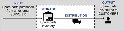
Dealing with the key characteristics, the DSS is developed for managers and practitioners interested in two-echelon SCs, where spare parts are bought from an external supplier (not produced internally), stored in one or more DCs, and distributed to fulfil the product demand at multiple customer locations. Hence, the control volume underlying this study is shown in Figure 1, where the final customer may also be a subsequent retailer, as reported by Fathi et al. (2021).

Figure 1. Control volume considered to develop this study (within the dashed rectangle).

The figure depicts the control volume considered to develop the mathematical model and achieve the decision support system.

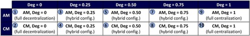
The proposed DSS supports managers and practitioners in choosing between ten spare parts SC designs, derived by combining two manufacturing technologies (AM and CM) with five spare parts SC configurations (ranging from centralisation to decentralisation passing through three hybrid configurations). A schematic representation of the five SC configurations considered is depicted in Figure 2, considering the example of a company purchasing spare parts from a supplier and serving six customers. The different spare parts SC configurations are identified through a parameter called ‘degree of centralisation’ ($\mathrm{Deg}$). Such parameter, based on the paper by Gregersen and Hansen (2018), is equal to one in the case of full centralisation, while it is the ratio between the number of DCs ($\mathrm{\#DC}$) able to answer customers’ demand and the number of customers to be served ($\mathrm{\#customers}$) in hybrid and decentralised SC configurations (Equation (1)). (1) $\begin{array}{rl}\mathrm{Deg}& =\mathrm{degree}\mathrm{of}\mathrm{centralisation}\\ & =\{\begin{array}{l}1\mathrm{full}\mathrm{centralised}\mathrm{SC}\mathrm{configuration}\\ 1-\frac{\mathrm{\#}\mathrm{DC}}{\mathrm{\#}\mathrm{customers}}\mathrm{else}\end{array}\end{array}$(1) As can be seen from Figure 2, the five different spare parts SC configurations considered in this work are those with $\mathrm{Deg}$ equal to 0 (decentralised configuration), 0.25 (hybrid configuration), 0.50 (hybrid configuration), 0.75 (hybrid configuration), and 1 (centralised configuration), and this choice was made to cover the range of possible SC configurations well. As an example, Figure 2 provides a schematic representation of the SC configurations considered in the case of a two-echelon SC serving six customers. In Figure 2, different locations are analysed for spare parts DCs. Instead, the supplier of the DCs is not shown, being represented by dashed arrows to indicate that it is out of control volume, and that we are not interested in its geographical location, but only in its average lead time.

Figure 2. Schematic representation of the five SC configurations considered. $\mathit{Deg}$ equal to 0 corresponds to a decentralised SC configuration, $\mathit{Deg}$ equal to 1 is a centralised configuration, and the values in between are hybrid SC configurations. The picture considers an example of a two-echelon SC serving six customers.

The figure shows a schematic representation of the five supply chain configurations examined to develop the decision support system. The five configurations vary based on the degree of centralization of the supply chain, which can assume value zero (that is full decentralisation), value one (that is full centralisation), three values (that are 0.25, 0.50, or 0.75), that correspond to an hybrid supply chain configuration.

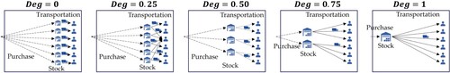
Figure 3, then, summarises the ten different spare parts SC designs considered by the DSS.

Figure 3. Matrix of the spare parts SC designs considered in the DSS.

The figure depicts a mtrix which summarises all the the supply chain design cosidered to perform the analysis and develop the decision support system. The ten supply chain design can assume all the integer numbers between 1 and 10. Odd numbers refer to supply chains delivering AM spare parts, while even numbers refer to CM supply chains. Moreover, numbers 1 and 2 refer to decentralised supply chains, numbers 9 and 10 consider centralised supply chains, while numbers 3 to 8 imply hybrid supply chains (with a degree of centralisation equal to 0.25, 0.50, or 0.75).

Concerning the assumptions made in the development of the DSS, these are listed below.

1. A single external supplier is assumed based on the work by Farahani et al. (2015), who, based on the fact that several suppliers offer similar products, indicated that it is more efficient to consider a single supplier to serve subsequent DCs;

2. Spare parts are assumed to be purchased from an external supplier (not produced in-house); this means that the costs of purchasing spare parts include all the costs that the supplier incurs. These costs include the costs of producing spare parts (also considering quality control activities), the fixed costs of AM/CM equipment, the costs of digitalising AM items, thus converting 2D drawings into 3D designs, and the profit margins that suppliers want to achieve (Pour et al. 2016);

3. Based on Tapia-Ubeda et al. (2020), no capacity constraints are considered for the supplier’s warehouse and the DCs. Hence, it is assumed that each facility is able to keep inventories without space limitations;

4. Lead times are deterministic, as suggested by Schwarz (1973) and Cohen, Kleindorfer, and Lee (1988), while spare parts demand is stochastic, following a Poisson distribution as suggested, e.g. by Stoll et al. (2015) and Sherbrooke (1968);

5. Decentralised DCs are considered to be geographically equidistant from the customer: in such a way that the DCs are characterised by the same lead times and transportation costs. Moreover, the transportation costs in decentralised SC designs are considered negligible since each decentralised DC is supposed to be positioned close to the specific customer that it serves;

6. No reverse logistics (possibility of repairing and reusing broken spare parts) is considered, as suggested by Zijm, Knofius, and van der Heijden (2019), since the focus of this study is not the problem of sustainability in the SCs, but rather the SC design;

7. No lateral transhipments are admitted, as shown by Schwarz (1973);

8. Since the focus of this study is not the problem of sustainability in the SCs, but rather the SC design, no environmental effects of different SC designs are assessed. For example, CO2 emitted during transportations is neglected;

9. Only variable costs are considered (see Section 1), not assessing initial investment costs in facilities, or assets;

10. Spare parts transportation costs are calculated by assuming that only one spare part is distributed per trip. This hypothesis is considered acceptable because spare parts demand follows a Poisson distribution, also known as the law of rare events.

In addition, to develop the DSS, some modelling and spare parts management choices were taken, which are listed in the following remarks.

1. Warehouses are managed according to a continuous inventory control policy. Given the nature of lead times and demand, the selected inventory policy is (s,Q), where $s$ is the reorder level and $Q$ is the economic order quantity. Indeed, Fathi et al. (2021), Ivanov (2021), and Sapna Isotupa (2006) suggest such an inventory control policy as the optimal one in the case of stochastic demand and deterministic lead time;

2. The average annual demand of one customer is known, as well as the number of customers to be served, as shown by Cohen, Kleindorfer, and Lee (1988);

3. The duration of the period considered to develop the analysis is one year, as done by Daskin, Coullard, and Shen (2002). It is worth mentioning that this information is not a simplifying assumption, but it is here listed to underline that the total costs of SCs are calculated over a time horizon of one year, as well as the values of (s, Q) needed to control the inventory replenishment of DCs. The mathematical model and the analysis provided below could also be repeated by considering smaller or larger time horizons;

4. The risk of obsolescence is considered included within the holding cost rate. This choice is in line with what reported by Khajavi, Partanen, and Holmström (2014), who showed that the inventory obsolescence cost in a DC can be calculated as a function of the inventory level and of an annual part obsolescence rate. Therefore, in the present study, the annual part obsolescence rate is considered contained within the holding cost rate;

5. SKUs are supposed to be producible with both AM and CM. This assumption is introduced to allow the comparison between SCs where the distributed spare parts are of AM or CM type, thus answering the second research question (RQ2). However, in the case that some parts are not producible with AM technologies (as shown by Zijm, Knofius, and van der Heijden (2019)), it is possible to use the mathematical model here proposed only by comparing SC designs with CM items (numbers 2, 4, 6, 8, and 10 in Figure 3). Viable method for selecting spare parts suitable for AM are offered by Chaudhuri et al. (2021) and (Frandsen et al. 2020);

6. A single-item approach is adopted, choosing for each individual SKU the optimal SC design. This derives from the works by Stoll et al. (2015) and Cohen, Agrawal, and Agrawal (2006), who suggested that an effective SC configuration should adopt a single-item approach to ensure the optimal distribution of each individual SKU.

Now that the key characteristics of the proposed DSS and the assumptions made have been described, the four main steps followed to develop the DSS can be discussed. In Step 1, a mathematical model to compare the cost-effectiveness of the ten spare parts SC designs was developed. Then, in Step 2, an analysis of variance (ANOVA) was performed to determine the most relevant input parameters of the mathematical model, thus checking if any of them have a negligible impact on the selection of the optimal SC design. In Step 3, a parametric analysis was performed to investigate a sample of 10,000 realistic spare parts SC scenarios (i.e. spare parts SCs characterised by different spare parts demand, purchasing costs, transportation costs, backorder costs, and required service level) collected by varying the most relevant input parameters of the mathematical model (emerging from Step 2). Finally, in Step 4, the DSS was obtained in the form of a decision tree by leveraging a machine learning algorithm (specifically a decision tree algorithm) fed with the results of the parametric analysis. Each step is described in detail below in a specific section.

3.1 Mathematical model

In Step 1 of the development of the DSS, a mathematical model was established to compare the costs of the considered spare parts SC designs, thus allowing the optimal design to be identified. Table 1 lists the model input parameters.

Table 1. Input parameters for the mathematical model.

Input parameter	Description	Unit measure
$i$	Considered SC design. $i$ can assume integer values between 1 and 10 according to Figure 3	[–]
$j$	Manufacturing technology of the purchased spare parts. $j$ can be AM or CM	[–]
$\mathrm{\#customers}$	Number of customers served by the company	[–]
$\mathrm{ELTSL}$	Desired expected lead time service level$\mathrm{ELTSL}$	[–]
${\overline{D}}_{1\mathrm{customer}}$	Average annual demand for SKU emitted by one customer	[units/time]
$\mathrm{De}{g}_i$	Degree of centralisation in SC configuration $i$. It assumes a specific value according to Figure 3^a	[–]
$\mathrm{etcentra}{l}_i$	Unitary external transportation cost from the central DC to customers. It only refers to centralised SC configurations ($i=9$ or$i=10$)	[€/transportation]
$\mathrm{uback}$	Unitary cost of one backorder of SKU	[€/backorder]
$L_j$	Lead time needed by the supplier to deliver the j-th SKU to DCs	[time]
$u{c}_j$	Unitary cost of purchasing the j-th SKU from the supplier	[€/unit]
$\mathrm{mh}$	Hourly labour cost	[€/time]
$\mathrm{ot}$	Average time needed to send one replenishment order	[time]
$h_{\mathrm{\%}}$	Holding cost rate for keeping inventory of SKU	[€/time*unit]

^a $\mathrm{De}{g}_i$ is 0 if $i$ is equal to 1 or 2, is 0.25 if $i$ is equal to 3 or 4, is 0.5 if $i$ is equal to 5 or 6, is 0.75 if $i$ is equal to 7 or 8, while is 1 if $i$ is equal to 9 or 10.

According to the assumption, the costs are related to a single item, and therefore the optimal spare parts SC design is the one that minimises the spare parts SC total costs $\left(\mathrm{Cto}{t}_i\right)$ for a single SKU (Equation (2)). (2) $min\left[\mathrm{Cto}{t}_i\right]\mathrm{with}i=1,2,\dots ,10$(2) where $\mathrm{Cto}{t}_i$ is calculated according to Equation (3) as the sum of the costs of purchasing spare parts ($P{C}_{i,j}$), placing supply orders ($O{C}_{i,j}$), holding inventory ($H{C}_{i,j}$), transporting spare parts from DCs to customers ($\mathrm{ET}{C}_i$), and backorders ($B{C}_i$). (3) $\mathrm{Cto}{t}_i=P{C}_{i,j}+O{C}_{i,j}+H{C}_{i,j}+\mathrm{ET}{C}_i+B{C}_i$(3)

Specifically:

 $P{C}_{i,j}$ (the total cost of purchasing spare parts from the external supplier for a specific SC design $i$), according to Equation (4), is given by the product between the unitary cost of the spare part ($u{c}_j$), the number of DCs in the SC ($\mathrm{\#D}{C}_i$, Equation (5)), and the average annual demand in each DC ($\overline{\mathrm{Dto}{t}_i}$, Equation (6)). (4) $\begin{array}{rl}P{C}_{i,j}& =u{c}_j\ast \overline{\mathrm{Dto}{t}_i}\ast \mathrm{\#D}{C}_i\end{array}$(4) (5) $\begin{array}{rl}\mathrm{\#D}{C}_i& =\{\begin{array}{l}{\left[\left(1-\mathrm{De}{g}_i\right)\ast \mathrm{\#customers}\right]}^{+}\mathrm{if}i=1,2,\dots ,8\\ 1\mathrm{if}i=9,10\end{array}\end{array}$(5) (6) $\begin{array}{rl}\overline{\mathrm{Dto}{t}_i}& =\{\begin{array}{l}\left(\frac{{\overline{D}}_{1\mathrm{customer}}\ast \mathrm{\#}\mathrm{customers}}{\mathrm{\#}D{C}_i}\right)\mathrm{if}i=1,2,\dots ,8\\ \left(\mathrm{\#customers}\ast {\overline{D}}_{1\mathrm{customer}}\right)\mathrm{if}i=9,10\end{array}\end{array}$(6) $O{C}_{i,j}$ (the total cost of placing orders for replenishing DCs’ inventories), according to Equation (7), is given by the product between the unitary cost of placing one order ($\mathrm{oc}$, Equation (8)), the average number of orders ($\mathrm{\#order}{s}_{i,j}$, Equation (9)), and the number of DCs ($\mathrm{\#D}{C}_i$). (7) $\begin{array}{rl}O{C}_{i,j}& =\left(\mathrm{oc}\ast \mathrm{\#order}{s}_{i,j}\right)\ast \mathrm{\#D}{C}_i\end{array}$(7) (8) $\begin{array}{rl}\mathrm{oc}& =\mathrm{mh}\ast \mathrm{ot}\end{array}$(8) (9) $\begin{array}{rl}\mathrm{\#order}{s}_{i,j}& =\frac{\overline{\mathrm{Dto}{t}_i}}{Q_{i,j}}\end{array}$(9) where $Q_{i,j}$ is the economic order quantity for replenishing SKUs in DCs calculated using Wilson’s formula (Stoll et al. 2015) (Equation (10)), and $h_j$ is the unitary holding cost in each DC (Equation (11)). (10) $\begin{array}{rl}{Q}_{i,j}& =\sqrt{\frac{2\ast \overline{\mathrm{Dto}{t}_i}\ast \mathrm{oc}}{h_j}}\end{array}$(10) (11) $\begin{array}{rl}{h}_j& =u{c}_j\ast h_{\text{\%}}\end{array}$(11) $H{C}_{i,j}$ (the total holding cost), according to Equation (12), is given by the product between the unitary holding cost, the average inventory in each DC ($I_{i,j}$, Equation (13)), and the number of DCs ($\mathrm{\#D}{C}_i$). (12) $\begin{array}{rl}H{C}_{i,j}& =\left(h_j\ast I_{i,j}\right)\ast \mathrm{\#D}{C}_i\end{array}$(12) (13) $\begin{array}{rl}{I}_{i,j}& =\frac{Q_{i,j}}{2}+S{S}_{i,j}\end{array}$(13) Where $S{S}_{i,j}$ are the safety stocks in each DC, corresponding to the smallest value that satisfies Equation (14), thus compensating demand fluctuations (Equation (15)) and avoiding stock-outs at least to ensure the desired service level. (14) $\begin{array}{rl}& 1-\sum _{n=0}^{S{S}_{i,j}-1}\left[\frac{{\left(\overline{\mathrm{Dtot}\mathrm{in}\mathrm{lead}\mathrm{tim}{e}_{i,j}}\right)}^n}{n!}\ast e^{-\overline{\mathrm{Dtot}\mathrm{in}\mathrm{lead}\mathrm{tim}{e}_{i,j}}}\right]\\ & \ge \left(1-\mathrm{ELT}\mathrm{SL}\right)\end{array}$(14) (15) $\begin{array}{rl}& \overline{\mathrm{Dtot}\mathrm{in}\mathrm{lead}\mathrm{tim}{e}_{i,j}}=\overline{\mathrm{Dto}{t}_i}\ast L_j\end{array}$(15) $\mathrm{ET}{C}_i$ (the total transportation cost to deliver spare parts from DCs to customers), according to Equation (16), is given by the product between the unitary external transportation costs ($e{t}_i$, Equation (17)), the average demand ($\overline{\mathrm{Dto}{t}_i}$), and the number of DCs ($\mathrm{\#D}{C}_i$). (16) $\begin{array}{rl}\mathrm{ET}{C}_i& =\left(e{t}_i\ast \overline{\mathrm{Dto}{t}_i}\right)\ast \mathrm{\#D}{C}_i\end{array}$(16) (17) $\begin{array}{rl}e{t}_i& =\{\begin{array}{l}\mathrm{et}\mathrm{decentra}{l}_i\mathrm{if}i=1,2,\dots ,8\\ \mathrm{et}\mathrm{centra}{l}_i\mathrm{if}i=9,10\end{array}\end{array}$(17) where the unitary external transportation costs for decentralised and hybrid configurations ($\mathrm{etdecentra}{l}_i$) is defined according to Equation (18) (for more information on Equation (18) see Appendix A). (18) $\mathrm{et}\mathrm{decentra}{l}_i=\mathrm{et}\mathrm{centra}{l}_i\ast f\left(\mathrm{De}{g}_i\right)$(18) Finally, $B{C}_i$ (the total cost of backorders), according to Equation (19), is given by the product between the unitary backorder cost ($\mathrm{uback}$), the average number of backorders ($\mathrm{\#backorder}{s}_i,$Equation (20)), and the number of DCs ($\mathrm{\#D}{C}_i$). (19) $\begin{array}{rl}B{C}_i& =\left(\mathrm{uback}\ast \mathrm{\#backorder}{s}_i\right)\ast \mathrm{\#D}{C}_i\end{array}$(19) (20) $\begin{array}{rl}\mathrm{\#backorder}{s}_i& =[\left(1-\mathrm{ELT}\mathrm{SL}\right)\ast \overline{\mathrm{Dto}{t}_i}{]}^{+}\end{array}$(20)

3.2. ANOVA analysis

In Step 2 of the development of the DSS, an analysis of variance (ANOVA) was used to define if all the input parameters (Table 1) strongly impact the selection of the optimal SC design or if any of them have a negligible effect. To this end, a preliminary parametric analysis was first carried out. In the preliminary parametric analysis, the parameters $\mathrm{mhmh}$, $\mathrm{ot}$, and $h_{\mathrm{\%}}$ in Table 1 were assumed fixed and equal to 30 €/h, 10 min, and 25% respectively, while the remaining independent variables of Table 1 (excluding $i$, which already had predefined values, and differentiating cost items in the case of AM or CM manufacturing) were associated with a range of realistic discrete admissible values (Table 2). As shown in Table 2, three values were considered for each parameter, where two of them (the extremes) were defined by consulting the sources in the last column of Table 2, while the third value was taken as the intermediate number. This resulted in a total of 729 different combinations of the input parameters (each combination of input parameters is what we refer to as ‘scenario’), which were then used in the mathematical model of Step 1 to determine the optimal spare parts SC design for each scenario. Finally, the results were subjected to an ANOVA using Minitab software, where the parameters listed in the first column of Table 2 were indicated as input factors, while the optimal SC design outcomes were indicated as responses. It is worth mentioning that the ANOVA was performed allowing variables to assume only three discrete values to obtain easily understandable graphs in which the trend of the curves could be immediately recognised, thus revealing the impact of the parameters on the decision.

Table 2. Parameters and values of discretised parametric analysis.

Input parameter	Admissible values	Unit measure	Source used to define the admissible values
$\mathrm{\#customers}$	5; 53; 100	[–]	Authors’ experience^a
$\mathrm{ELTSL}$	0.85; 0.92; 0.99	[–]	Authors’ experience
${\overline{D}}_{1\mathrm{customer}}$	1; 4; 7	[units/year]	(Knofius et al. 2021)
$\mathrm{etcentra}{l}_i$	100; 1,050; 2,000	[€/transportation]	Authors’ experience
$\mathrm{uback}$	1,000; 50,500; 100,000	[€/backorder]	(Peron et al. 2021)
$L_{\mathrm{AM}}$	1; 2.5; 4	[weeks]	(Knofius et al. 2021)
$L_{\mathrm{CM}}$	4; 15; 26	[weeks]	(Knofius et al. 2021)
$u{c}_{\mathrm{AM}}$	100; 1,300; 2’500	[€/unit]	(Knofius et al. 2021)^b
$u{c}_{\mathrm{CM}}$	10; 1,255; 2,500	[€/unit]	(Knofius et al. 2021)^c

^a The over twenty years' experience of some of the authors in the field of logistics and spare parts management combined with the consultation of expert staff from spare parts distribution companies make these assumptions reliable.

^b Knofius et al. (2021) considered 1197 €/unit. We have assumed a wider range.

^c Knofius et al. (2021) reported that the cost of CM parts is typically lower than AM ones, but this does not always hold true (it depends on the part complexity). Hence, we assumed a minimum value lower than AM, but the same upper limit.

3.3. Parametric analysis

After performing the ANOVA, parameters whose impact is negligible concerning the suggestion of the optimal SC design were excluded from the study. Conversely, the input parameters with a significant influence on the results were considered in Step 3 of the development of the DSS.

Aiming to obtain a DSS in the form of a decision tree, a dataset was required to feed and train the decision tree algorithm. For this reason, in Step 3, another parametric analysis was developed to collect and investigate a sample of 10,000 realistic spare parts SC scenarios (with different demands, costs, and service levels). Overall, the process of obtaining the data used to conduct this parametric analysis can be summarised as follows. First, the parameters $\mathrm{mh}$, $\mathrm{ot}$ and $h_{\mathrm{\%}}$ in Table 1 were again assumed fixed (considering the same values mentioned in Section 3.2), while the independent non-negligible parameters resulting from Step 2 were associated with a range of realistic admissible values defined within upper and lower limits. As upper and lower limits, the same extreme values of the ranges in Table 2 were chosen. However, unlike the parametric analysis of Step 2, here the parameters were not allowed to take on only three values, but rather intermediate values were assigned using the Sobol quasi-random low discrepancy sequence (Burhenne, Jacob, and Henze 2011). Hence, each parameter ($\mathrm{par}$) was represented as a set of values uniformly distributed over a range determined according to Equation (21). (21) $\mathrm{par}=\mathrm{pa}{r}_{\mathrm{lower}\mathrm{limit}}+\mathrm{Sobol}\cdot \left(\mathrm{pa}{r}_{\mathrm{upper}\mathrm{limit}}-\mathrm{pa}{r}_{\mathrm{lower}\mathrm{limit}}\right)$(21) Table 3 reports the range of admissible values for the Sobol-based parametric analysis.

Table 3. Values considered in the Sobol-based parametric analysis. The range extreme values are based on Table 2.

Input parameter	Range of admissible values	Unit measure
$\mathrm{\#customers}$	integers between 5 and 100	[–]
$\mathrm{ELTSL}$	floats between 0.85 and 0.99	[–]
${\overline{D}}_{1\mathrm{customer}}$	integers between 1 and 7	[units/year]
$\mathrm{etcentra}{l}_i$	floats between 100 and 2,000	[€/transportation]
$\mathrm{uback}$	floats between 1,000 and 100,000	[€/backorder]
$L_{\mathrm{AM}}$	integers between 1 and 4	[weeks]
$L_{\mathrm{CM}}$	integers between 4 and 26	[weeks]
$u{c}_{\mathrm{AM}}$	floats between 100 and 2,500	[€/unit]
$u{c}_{\mathrm{CM}}$	floats between 10 and 2,500	[€/unit]

Then, by randomly mixing the values of the input parameters, a sample of 10,000 scenarios was collected, where, for each scenario, the mathematical model of Step 1 (Section 3.1) was applied, determining the optimal SC design.

It should be noted that the Sobol quasi-random low discrepancy sequence was chosen based on the study by Burhenne, Jacob, and Henze (2011), who report that, when studying problems with a large number of input variables, the Sobol sequence is expected to be more effective in exploring the input variable space in comparison to other sampling strategies (i.e. discrete sampling, Monte Carlo, or Latin Hypercube).

3.4. Decision tree

Finally, in Step 4, the DSS in the form of a decision tree was generated, constituting a guideline for managers and practitioners to understand which spare parts SC design is the optimal (more cost-effective) for them. To develop such DSS, a decision tree algorithm was used. A decision tree algorithm is a supervised classification technique, and it predicts the class to which an item belongs based on a given set of attributes (Nugroho, Adji, and Fauziati 2015). Here, the results of the parametric analysis (Step 3) were used as the dataset for training the decision tree algorithm (using Python's Sklearn library), where for each scenario:

• The values of the non-negligible input parameters were given as input attributes.

• The optimal spare parts SC design determined by applying the mathematical model was indicated as the final class label that the decision tree algorithm should learn to predict.

Therefore, the decision tree was obtained as follows. Starting at a root node, the dataset was recursively split into binary subsets (branches) based on the Gini diversity index ($\mathrm{gdi}$, Equation (22)), where $K$ is the number of class labels (the ten spare parts SC designs defined in Figure 3), and $p\left(k\right)$ is the probability of picking the data point with the class$k$ (Shaheen, Zafar, and Ali Khan 2020). $\mathrm{gdi}$ measures the probability of a given data point from the dataset being wrongly classified when it is randomly chosen (Arena et al. 2022). Hence, $\mathrm{gdi}=0$ means that all data points of the dataset belong to a certain class, while $\mathrm{gdi}=1$ implies that the data points are randomly distributed across different classes. (22) $\mathrm{gdi}=1-\sum _{k=1}^{K}p(k{)}^2$(22) At each node of the tree, an attribute and its cut point were chosen to generate two branches with the aim of minimising Equation (23), thus identifying the split which provided the maximum purity. (23) $min\left(\frac{n_{\mathrm{left}}}{n}\mathrm{gd}{i}_{\mathrm{left}}+\frac{n_{\mathrm{right}}}{n}\mathrm{gd}{i}_{\mathrm{right}}\right)$(23) In Equation (23), $n$ is the number of data points in the original node, $n_{\mathrm{left}}$ is the number of data points in the new node on the left branch, $n_{\mathrm{right}}$ is the number of data points in the new node on the right branch, $\mathrm{gd}{i}_{\mathrm{left}}$ is the Gini diversity index in the new node on the left branch, and, finally, $\mathrm{gd}{i}_{\mathrm{right}}$ is the Gini diversity index in the new node on the right branch (Sgarbossa et al. 2021). The elements at the end of the tree, obtained after the last branch split, are called leaves, and the number of splits performed coincides with the number of levels (depth) of the tree.

Seeking to generate a user-friendly DSS, the decision tree was pruned by imposing a maximum depth ($\mathrm{Dmax}$, maximum number of splits of the starting dataset into sub-branches before reaching a leaf). This pruning activity was also useful to avoid the over-fitting problem when generating the tree (Morgan et al. 2003). For the pruning purpose, a sensitivity analysis of the total accuracy ($A$) of the decision tree was performed by imposing different values for $\mathrm{Dmax}$, and determining the resulting $A$ calculated as the ratio between the number of correct predictions ($\mathrm{\#correctprediction}{s}_{\mathrm{tree}}$) and the number of total predictions ($\mathrm{\#prediction}{s}_{\mathrm{tree}}$, initial dataset size) (Equation (24)). (24) $\mathit{A}=\frac{\mathrm{\#}\mathrm{correct}\mathrm{prediction}{s}_{\mathrm{tree}}}{\mathrm{\#}\mathrm{prediction}{s}_{\mathrm{tree}}}$(24) The decision tree representing a trade-off between the accuracy of predictions and user-friendliness was then proposed as a DSS. Finally, the effectiveness of the selected decision tree was evaluated based on three key performance indicators (KPIs) related to the leaves of the tree. The first KPI is the accuracy of each leaf ($a$, Equation (25)), given by the ratio between the number of correct predictions ($\mathrm{\#correctprediction}{s}_{\mathrm{leaf}}$) and the number of total predictions in the leaf ($\mathrm{\#prediction}{s}_{\mathrm{leaf}}$). The second KPI is the number of elements reaching each leaf $(p$, Equation (26)), given by the ratio between the number of elements classified within that leaf ($\mathrm{\#prediction}{s}_{\mathrm{leaf}}$) and the number of total elements to be classified $\left(\mathrm{\#prediction}{s}_{\mathrm{leaf}}\right)$. The last KPI is the average percentage increase in cost that occurs when the wrong option is selected in the leaf ($\text{c}$, Equation (27)), obtained as the arithmetic mean of the cost increase generated by each wrong prediction. (25) $\begin{array}{rl}a& =\frac{\mathrm{\#}\mathrm{correct}\mathrm{prediction}{s}_{\mathrm{leaf}}}{\mathrm{\#}\mathrm{prediction}{s}_{\mathrm{leaf}}}\end{array}$(25) (26) $\begin{array}{rl}p& =\frac{\mathrm{\#}\mathrm{prediction}{s}_{\mathrm{leaf}}}{\mathrm{\#}\mathrm{prediction}{s}_{\mathrm{tree}}}\end{array}$(26) (27) $\begin{array}{rl}c& =\frac{\begin{array}{c}{\sum }_{k=1}^{\mathrm{\#}\mathrm{wrong}\mathrm{predicion}{s}_{\mathrm{leaf}}}\\ \left(\left|\frac{\text{cost}\mathrm{of}\mathrm{wrong}\mathrm{prediction}-\mathrm{cost}\mathrm{of}\mathrm{correct}\mathrm{predictio}{n}_k}{\mathrm{cost}\mathrm{of}\mathrm{correct}\mathrm{predictio}{n}_k}\right|\ast 100\right)\end{array}}{\mathrm{\#}\mathrm{uncorrect}\mathrm{prediction}{s}_{\mathrm{leaf}}}\end{array}$(27)

4. Results and discussion

As mentioned in Section 3, having developed the mathematical model to compare the costs of different SC designs (Step 1, Section 3.1), the next step conducted was the development of an ANOVA (Step 2, Section 3.2), whose results are shown in Figure 4.

Figure 4. Results of the ANOVA (Main Effects Plots) for the optimal SC design.

The figure depicts the results of the ANOVA analysis conducted. Nine graphs are represented (one for each independent variable affecting the proposed mathematical model). The plots prove that the impact of three out of nine variables (lead time AM, lead time CM, and the expected service level) can be considered negligible in respect to the optimal supply chain design suggested by the mathematical model.

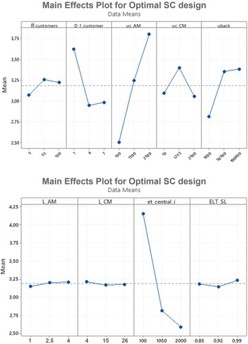
Figure 4 proves that three out of the nine input parameters considered (Table 2) have a negligible impact on the process of selecting the optimal spare parts SC design. In fact, when varying the three discrete values assumed by $L_{\mathrm{AM}}$, $L_{\mathrm{CM}}$, and $\mathrm{ELTSL}$, the curve obtained in the Main Effects Plots relative to the mean of the optimal SC designs is almost horizontal. Therefore, the effect of the parameters $L_{\mathrm{AM}}$, $L_{\mathrm{CM}}$, and $\mathrm{ELTSL}$ on the selected spare parts SC design can be considered null. On the contrary, the remaining parameters show a non-negligible impact on this decision-making process.

Given the ANOVA results, the $L_{\mathrm{AM}}$, $L_{\mathrm{CM}}$, and $\mathrm{ELTSL}$ parameters were not considered for building the DSS, being excluded from the implementation of the parametric analysis (Step 3 in Section 3.3). Instead, the remaining six parameters were associated with Sobol values as indicated in Table 3. Then, such values were randomly joined together to create a sample of 10,000 realistic spare parts SC scenarios, and for each scenario the optimal spare parts SC design was determined through the mathematical model of Section 3.1. As described in Section 3.4, the results were then used to feed a decision tree algorithm, where the values assumed by the input variables in the different scenarios were used as input attributes, while the identifier of the optimal spare parts SC designs was indicated as the final class label.

Aiming to obtain a DSS that is both easy-to-use (that corresponds to an easy-to-read decision tree) and accurate, we carried out a sensitivity analysis of the total accuracy A of the decision to determine how to prune the branches (Figure 5). Based on the results depicted in Figure 5, we decided to use as DSS the decision tree with $\mathrm{Dmax}=4$ (red circle in Figure 5) since it represents a trade-off between user-friendliness and accuracy. Figure 6 shows the decision tree with $\mathrm{Dmax}=4$.

Figure 5. Sensitivity analysis on the accuracy ($\mathit{A}$) of the decision tree.

The figure depicts by means of a graph the sensitivity analysis conducted to study the trend of the decision tree accuracy (y-axes) when varying the maximum depth of the tree (x-axes).

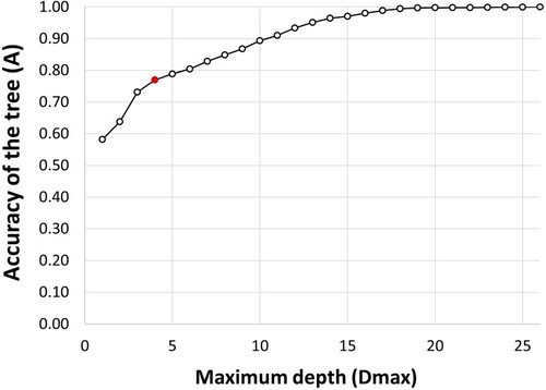
Figure 6. Decision tree with a maximum depth of 4 levels ($\mathit{Dmax}=4$).

The figure depicts the 4-levels decision tree provided as a decision support system. Threshold values are reported for the independent variables, to guide managers and practitioners in choosing the optimal supply chain design.

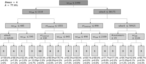
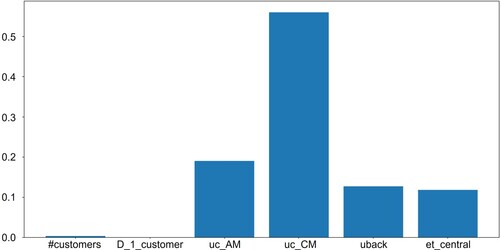
It is interesting noting that not all the six non-negligible parameters identified from the ANOVA analysis are used in the decision tree (${\overline{D}}_{1\mathrm{customer}}$ is missing), suggesting that some parameters are more important on the optimal SC design choice than others. This is confirmed by Figure 7, that shows the relative importance of the independent parameters on the choice of the optimal SC design (the relative importance is calculated first combining the changes in the Gini Diversity Index weighted by the node probability due to splits at each parameter, then dividing the sum by the number of branch nodes (Lolli et al. 2022)). From the relative importance, in fact, it emerges that $u{c}_{\mathrm{CM}}$ and $u{c}_{\mathrm{AM}}$ are the two parameters that influence the most the choice of the optimal SC design (the first decision on the decision tree is in fact made on $u{c}_{\mathrm{CM}}$), followed by $\mathrm{uback}$ and $\mathrm{etcentra}{l}_i$. The relative importance of ${\overline{D}}_{1\mathrm{customer}}$ is instead low, meaning that this parameter has a weaker impact on the SC design decision, and for this reason, when pruning the tree, ${\overline{D}}_{1\mathrm{customer}}$ does not appear in Figure 6.

Figure 7. Relative importance of the independent parameters on the decision of the optimal SC design.

The figure presents a histogram, showing the relative importance (y-axes) of the model independent variables (x-axes), where a higher relative importance means that such variable strongly affect the optimal SC design suggested by the decision support system.

Moreover, the decision tree in Figure 6, shows that the most recommended spare parts SC designs in the DSS are those with AM/CM and $\mathrm{De}{g}_i=0.25$ (spare parts SC designs 3–4), which are suggested in eleven out of sixteen leaves of the tree. Given the frequent cost-effectiveness of such spare parts SC designs, this study demonstrates the importance of considering hybrid spare parts SC configurations in the analysis, not only comparing centralised and decentralised spare parts SC configurations. In particular, spare parts SC design 3 with AM and $\mathrm{De}{g}_i=0.25$ is more cost-effective than the others whenever $u{c}_{\mathrm{CM}}$ is higher than 1,490 €/unit and the cost of one backorder ($\mathrm{uback}$) is higher than 38,175 €/backorder. In fact, in such a case, the unitary cost of purchasing AM spare parts is similar to or lower than the CM one, so an AM spare part SC design is usually preferable. In addition, in such a case, a hybrid spare parts SC configuration with a low degree of decentralisation (0.25%) reduces backorders by benefiting from the risk-pooling effect (the demand is aggregated in a few DCs) while keeping delivery times and costs lower than in fully centralised SC configurations.

Conversely, the leaves of the decision tree in Figure 6 do not include spare parts SC designs 5–9, indicating that, generally, SCs with $\mathrm{De}{g}_i$ of 0.50 and 0.75 are not cost-effective, as well as the total centralisation of AM spare parts. Moreover, Figure 6 shows the KPIs ($a$, $p$, and $c$, Section 3.4) of the decision tree with $\mathrm{Dmax}=4$, demonstrating that some leaves have very high accuracy ($a>$ 90%), which guarantees the reliability of the predictions, while others have low accuracy ($a<50$%), which seems insufficient to trust the DSS. However, the increase of cost ($c$) that managers and practitioners should pay in the case of a wrong decision is always less than 10% (often even below 5$\mathrm{\%}$) and this means that an incorrect prediction of the decision tree has an impact on the company’s economy which is almost negligible in respect to the one that the optimal spare parts SC design (correct prediction) would imply. Hence, the low value of $c$ makes it easier for managers and practitioners to accept the decisions suggested by the decision tree with $\mathrm{Dmax}=4$, even if the accuracy of the leaves is not very high. Meanwhile, in the Supplemental Material attached to this study, we also provide a second decision tree (with $\mathrm{Dmax}=15$), which guarantees more accurate predictions ($A=97\mathrm{\%}$), thus being useful for managers and practitioners to check the results of the DSS in Figure 6. We do not provide the decision tree with 100% accuracy (with $\mathrm{Dmax}=26$), but rather the tree on fifteen levels because, as reported by Morgan et al. (2003), a pruning reduces the overfitting problem, even if a slight reduction in the accuracy of the decision tree should be accepted.

The tree with $\mathrm{Dmax}=15$is less easy-to-use than the one with $\mathrm{Dmax}=4$, since fifteen concatenated questions should be answered before reaching a leaf, and the decision tree is split into several branches, making it difficult to identify the one relating to some specific input parameter conditions. For this reason, the Supplemental Material shows the decision tree with $\mathrm{Dmax}=15$ not in graphical form but rather as a Python code. In this way, managers and practitioners can incorporate the script into their company systems, thus automating the process of answering questions and quickly achieving the optimal spare parts SC design. In the Supplemental Material, spare parts SC designs 1, 2, 3, 4, and 10 are the most frequently suggested, confirming the accuracy of the decision tree with $\mathrm{Dmax}=4$. Moreover, the decision tree with $\mathrm{Dmax}=15$ finds some specific cases where designs 5, 6, 7, 8, and 9 are economically profitable.

Overall, aiming to provide managers and practitioners with an easy-to-use and reliable DSS, the decision tree with $\mathrm{Dmax}=4$ is selected as the main tool to support the choice process. However, the benefits of the two alternatives (both the decision tree with $\mathrm{Dmax}=4$ and the one with $\mathrm{Dmax}=15$) can be reaped as follows, using the decision tree with $\mathrm{Dmax}=15$ only when the reliability of the tree with $\mathrm{Dmax}=4$ is not sufficient. At first, the DSS constituted by the decision tree with $\mathrm{Dmax}=4$ can be consulted to receive an initial suggestion on the optimal spare parts SC design. Then, managers and practitioners can check the accuracy of the leaf in which the SKU managed by their company falls. Hence, two circumstances can occur:

• If the accuracy of the considered leaf is high, the result of the easy-to-use decision tree with $\mathrm{Dmax}=4$ can be trusted.

• Conversely, if the accuracy of the leaf is low, then managers and practitioners can proceed as follows. First, they should check the KPI $c$ and evaluate the increase of cost that they would have to pay in the case of a wrong decision. If they consider the increase of cost acceptable (it is often very low), then they can accept the decision tree prediction even if the accuracy is not very high. If, instead, they do not consider the increase of cost acceptable, they can then consult the decision tree with $\mathrm{Dmax}=15$ to get a more reliable result and be sure about the optimal spare parts SC design.

4.1. DSS application

The following case studies show the DSS application on the data provided by an Italian company which distributes bus spare parts to five main customers. Four DCs are currently available to stock more than 3,000 types of SKUs, and warehouse managers are in charge of the supply of items in each DC, for which they define the inventory control policies based on their algorithms and experience. The service level required by the company to meet customer requests for each spare part is equal to 95%. The company is an official partner of a well-known manufacturer of bus components, from whom it purchases all the stocks in the form of CM finished products (i.e. a single supplier serves all DCs). The company is recently considering performing a reconfiguration of its SC design, thus optimising the management of each SKU and the economic performance. Moreover, the company is interested in evaluating the possibility of buying AM spare parts instead of CM ones.

Here two case studies (A and B) are provided to illustrate different use cases of the DSS, referring to two different SKUs. For the selected SKUs, the lead-time ($L_{\mathrm{AM}}$) and unitary cost ($u{c}_{\mathrm{AM}}$) that the respective items would have if they were manufactured with AM were estimated by consulting AM experts from a company skilled in 3D printing. The results of both case studies are described below, showing: (i) the current SC design adopted by the company for the analysed SKU (AS-IS situation); (ii) the SC design recommended by the DSS; (iii) the SC design suggested by applying the mathematical model; (iv) the comparison of the previous information (i-iii) and a discussion on the results.

4.1.1. Case study A

Spare part A is an anti-particulate filter that is managed according to a hybrid SC design, where we can consider $\mathrm{Deg}=0.25$. Indeed, A-stocks are currently contained in three out of four DCs, since the remaining DC is small in size, and it is used to store only a few selected spare parts. The average demand of a customer for SKU A is 3 units/year and the cost of transporting one item from the DCs to a customer was estimated to be $\mathrm{etcentral}$ = 225 €/trip (based on the average distance between the DCs and the customers and the type of vehicle used for the deliveries, i.e. truck). Any stock-out of the warehouse for this SKU causes problems of unavailability to the customer's buses, which by law cannot travel without this filter. Therefore, the cost of a backorder was estimated at around 35,000 €/backorder in accordance with the company’s staff. The average lead time ($L_{\mathrm{CM}}$) guaranteed by the supplier for this SKU is 5 weeks, while the unitary purchase cost of this SKU ($u_{\mathrm{CM}}$) is 1,057 €. On the other hand, $L_{\mathrm{AM}}$ and $u_{\mathrm{AM}}$, were estimated to be 1.5 weeks and 1,370 €/unit, respectively.

Applying the decision tree with $\mathrm{Dmax}=4$ (DSS), the optimal SC design was identified as the number 4, corresponding to a hybrid configuration with $\mathrm{Deg}=0.25$ and CM spare parts. This choice was also confirmed by the mathematical model, which suggested as optimal the SC design characterised by $\mathrm{Deg}=0.25$, CM spares, and a total cost of around 37,000 €/year. Therefore, regarding the analysis of A-SKU, both the accuracy of the DSS (whose results matched those of the mathematical model), and the company choices (AS-IS situation) were validated.

4.1.1. Case study B

Spare part B is a specific type of connecting rod, currently managed according to an SC design of full centralisation ($\mathrm{Deg}=1$). Indeed, only one DC stocks inventory of B-items, serving the demand of all the customers. For SKU B, the average demand in the DC is equal to 5 units/year and the external transportation cost is still assumed equal to 225 €/trip. A stock-out of B-inventory causes problems of unavailability of the customer's vehicles. Hence, the cost of a backorder was estimated according to the know-how of the company’s staff equal to $\mathrm{uback}$ = 50,500 €/backorder. The average lead time ($L_{\mathrm{CM}}$) guaranteed by the supplier for this SKU is 4.5 weeks, while the unitary purchase cost of B ($u_{\mathrm{CM}}$) is 594 €. Finally, $L_{\mathrm{AM}}$ and $u_{\mathrm{AM}}$ were estimated to be 2.5 weeks and 1,052 €/unit, respectively.

The decision tree with $\mathrm{Dmax}=4$ suggests as optimal the SC design 1 (that is $\mathrm{Deg}=0$ and AM spares). Such a prediction is characterised by a risk percentage of cost increase due to an incorrect prediction equal to 6%, which is considered too high by the company. Therefore, to obtain a more accurate result, the decision tree with $\mathrm{Dmax}=15$ was also consulted. This decision tree suggests 4 as the optimal SC design (hybrid centralisation of CM spare parts and $\mathrm{Deg}=0.25$). Applying the mathematical model, the same result was achieved, recommending the SC design with $\mathrm{Deg}=0.25$ and CM items, which has a total cost of 77,942 €/year. Hence, the mathematical model gave the same result as the decision tree with $\mathrm{Dmax}=15$ and the DSS was validated. Ultimately, the company's AS-IS policy was not confirmed by the results of the case study, showing that the firm should consider adopting a hybrid SC configuration (instead of a centralised one), thus allocating B-stocks in three out of four DCs. However, the analysis revealed that the company is justified in sourcing CM B-parts because, for such a SKU, AM technology is less cost-effective than the CM one.

5. Conclusions

This paper proposes a DSS to support managers and practitioners in deciding on the optimal spare parts SC design (i.e. the decision about the optimal spare parts SC configuration combined with the choice of the manufacturing technology). The developed DSS guides the decision between five different spare parts SC configurations (centralisation, decentralisation, and three hybrid configurations) where spare parts could be manufactured either in AM or in CM, thus considering a total of ten different spare parts SC designs. To develop such a DSS, four main steps were followed: (i) a novel mathematical model was developed for determining and comparing the total costs of the different spare parts SC designs (including the cost of purchasing spare parts from external suppliers, cost of placing replenishment orders, holding costs, outbound transportation costs, and backorder costs); (ii) the most relevant input parameters for the mathematical model were determined through the development of an ANOVA; (iii) an extensive parametric analysis was performed where 10,000 different spare parts SC scenarios were developed, assigning values to the most relevant input parameters of the mathematical model (through the Sobol quasi-random low discrepancy sequence) and, for each scenario, the optimal spare parts SC design was identified using the mathematical model mentioned in (i); (iv) the parametric analysis was used to feed a decision tree algorithm to obtain the aforementioned DSS. Based on a sensitivity analysis, the decision tree was pruned by imposing a maximum depth of four levels to ensure a trade-off between user-friendliness and accuracy of predictions and avoid overfitting. The results of the decision tree show that some leaves have high accuracy, while others not. However, the results prove that even when the accuracy of the leaves is low, the average percentage of cost increase that managers and practitioners should pay in the case of incorrect prediction is always less than 10% (often below 5%). Therefore, the DSS leads to a robust choice since it selects the optimal spare parts SC design or, in the case of a wrong prediction, it always ensures opting for a spare parts SC design that does not have a negative impact on business economies (implying a total cost similar to that of the correct prediction). Meanwhile, as an additional tool for improving the accuracy of the decision-making process, this study also provides a supplementary decision tree with a maximum depth of fifteen levels (Supplemental Material), which is less easy-to-use than the four-level tree but has higher accuracy ($A=97\mathrm{\%}$), allowing managers and practitioners to verify the DSS results when needed.

The DSS developed herein represents the main contribution of this study, since nothing similar has been done before. In fact, to the best of our knowledge, no tool supporting managers and practitioners in deciding the optimal spare part SC design (i.e. spare parts SC configuration and manufacturing technology) has been developed so far. A decision tree algorithm is chosen here to build the DSS since it is renowned as a rapid and easy-to-use tool (Arena et al. 2022; Sgarbossa et al. 2021) and it allows the robustness of decisions to be measured with proper KPIs. Moreover, we have chosen to develop the DSS by exploiting a machine learning algorithm and data mining techniques since these are particularly useful when there are many variables impacting the system (Morgan et al. 2003; Orrù et al. 2020).

The main findings of the present study can be summarised as follows:

• The developed DSS is based on six input parameters ($\mathrm{\#customers}$, ${\overline{D}}_{1\mathrm{customer}}$, $\mathrm{etcentra}{l}_i$, $\mathrm{uback}$, $u{c}_{\mathrm{AM}}$, and $u{c}_{\mathrm{CM}}$), whose strong impact on the selection of the optimal spare parts SC design is demonstrated by the ANOVA. In contrast, the parameters $L_{\mathrm{AM}}$, $L_{\mathrm{CM}}$, and $\mathrm{ELTSL}$ were found to be negligible concerning the decision process investigated.

• The DSS is provided in the form of a decision tree with a maximum depth of four levels. Given the large number of parameters (six) impacting the choice of the optimal spare parts SC design, such a tree has a total accuracy of 77%. However, it guarantees to identify the spare parts SC design with the minimum cost or, in the case of a wrong prediction, a solution that deviates from the minimum cost by less than 10% (often less than 5%). Meanwhile, if this four-level decision tree is not considered sufficiently reliable as a DSS, the use of such a tree can be combined with that of a more complex and more reliable one (with fifteen levels), consulting this second tree only when the KPIs $a$ (leaf accuracy) and $c$ (cost increase due to incorrect prediction) of the four-level tree are low and high, respectively. The fifteen-level decision tree is provided here in the form of a Python code instead of a graphical diagram representation so that managers and practitioners can easily implement it in their company systems, thus automating its consultation.

• The spare parts SC designs most frequently suggested by the DSS are those with $\mathrm{De}{g}_i=0.25$ (designs 3 and 4), proving the importance of considering hybrid SC configurations in the analysis instead of focusing only on centralised and decentralised spare parts SC configurations. On the contrary, spare parts SC designs 5–9 are profitable only in very specific cases that the four-level tree does not consider.

It is worth noting that the results achieved are strictly related to spare parts SCs where the following assumptions can be considered valid: the spare parts demand follows a Poisson distribution, lead times are deterministic, warehouses have unlimited capacities, DCs are managed with (s,Q) inventory policy, and lateral transhipments, environmental impacts, reverse logistics, and spare parts obsolescence can be neglected. Besides, it is important to remember that the proposed DSS aims at optimising the allocation of individual SKUs considering only the variable costs of two-echelon SCs. However, all the mathematical formulas used to calculate the total costs of SC designs are reported in the present study. For this reason, if managers and practitioners do not consider the aforementioned simplifying assumptions compatible with the reality of their company, this problem can be overcome. In fact, although managers and practitioners cannot exploit the results of the DSS, they can be supported in their decisions by using the mathematical model herein provided and introduce or remove proper constraints, thus evaluating the real situation of their companies. For example, the assumption of decentralised DCs equidistant to the end customers can be easily removed by using the mathematical formulas of Section 3.1 and associating each DC with the specific transport cost calculated based on the exact distance that separates that DC from its end customer.

5.1. Theoretical and practical contributions

An efficient spare parts SC configuration improves the performance of a company in terms of economy, sustainability, and service level. Despite the importance of optimising the SC configuration, up to now, the problem of choosing between centralisation, decentralisation, and hybrid configurations has been overlooked in the literature. Specifically, the lack of quantitative methods to compare different SC configurations has led many spare parts dealers to optimise their SCs configurations based on their experience rather than on structured methods. Besides, recently, consideration has been given to the possibility of producing spare parts via AM, rather than CM, since AM technology can be more convenient under specific conditions. However, the decision on the optimal spare parts manufacturing technology has been hard to take for managers and practitioners since the existing literature lacks methods to quantitatively capture the differences between CM and AM SCs, providing evidence on when the adoption of AM spare parts can guarantee higher performance than the CM ones. In this context, the theoretical contribution of this paper is to overcome both these issues by providing a DSS and a mathematical model to understand under which conditions it is economically advantageous to have a centralised, decentralised, or hybrid SC configuration, also selecting the optimal manufacturing technology (AM or CM spare parts). As a corollary, the present work also lays the foundation for deeper scientific research regarding both the choice of the most cost-effective spare parts SC configuration (among centralisation, decentralisation, and hybrid SCs) and the choice between AM and CM spare parts.

At a practical level, the contribution of this study is to provide companies with a quick and user-friendly system (the DSS) for determining how to design spare parts SCs. The results of this study will help managers and practitioners in optimising for each SKU two aspects at the same time: the allocation of stocks inside company warehouses (choosing between centralisation, decentralisation, and hybrid configuration) and the items’ manufacturing technology (AM or CM).

An example of how managers and practitioners can benefit from the results of this study is the following. Considering the company's most critical SKUs, by establishing their optimal SC design through the proposed DSS (consulting the 4-depth decision tree once for each SKU), managers and practitioners can rapidly compare their actual SC management policy with the ideal situation recommended by the DSS. In case of discrepancies between the current policies and the optimal situation suggested by the DSS, managers and practitioners can change the management of spare parts within the SC. Hence, immediate economic benefits with a limited effort can be obtained, since the company can first check only its critical spare parts (for example those in class A of an ABC analysis), and then verify the other SKUs in a second moment. Moreover, only four questions need to be answered to compare the current company situation with the optimal SC design suggested by the decision tree.

5.2. Future research developments

Future developments of this research could be threefold: first, to repeat the study considering companies which produce spare parts internally, instead of purchasing them from external suppliers. Second, to optimise SC designs considering multiple SKUs instead of individual SKUs, thus introducing fixed costs (i.e. economic investments in facilities and assets such as AM printers) in the analysis. Finally, to consider using Random Forest instead of a decision tree algorithm to interpret the results of the Sobol-based parametric analysis, thus making the machine learning training more accurate and minimising overfitting issues.

In addition to this, some assumptions underlying the mathematical model could be relaxed or eliminated in future works. For instance, lead times could be considered stochastic instead of deterministic, obsolescence costs of spare parts could be considered as separate costs instead of being included in the holding cost rate, and sustainability issues could be included in the analysis. Moreover, the possibility to distribute multiple spare parts during each transportation could be considered, as well as the facilities capacity constraints.

6. Data availability statement

The authors confirm that the data supporting the findings of this study are available within the article [and/or] its supplementary material.

Disclosure statement

No potential conflict of interest was reported by the author(s).

Additional information

Notes on contributors

Alessandra Cantini

Alessandra Cantini is a Ph.D. student both at the University of Florence (UNIFI, Italy), and the Norwegian University of science and technologies (NTNU, Norway). Currently, she is studying topics related to spare parts management and logistics. Her research areas of interest include warehouse management, supply chain management, spare parts inventory management, warehouse safety assessment, and lean manufacturing.

Mirco Peron

Mirco Peron is a postdoctoral fellow at the Department of Mechanical and Industrial Engineering (MTP) at NTNU (Norway). His research interests are multi-disciplinary, and he is currently focusing on the impact of digitalisation and Industry 4.0 technologies on production and logistics systems. He is author and co-author of almost 50 publications in international congress and journals.

Filippo De Carlo

Filippo De Carlo is Associate Professor of Industrial Systems at the Department of Industrial Engineering (DIEF) at UNIFI (Italy) from 2006. He has been and he is involved in several European and National Projects. He is author and co-author of more than 50 publications on international congresses and journals. He is Associated Editor of an international journal. His research topics include industrial plant engineering, maintenance, industrial safety and risk, and energy management.

Fabio Sgarbossa

Fabio Sgarbossa is Full Professor of Industrial Logistics at the Department of Mechanical and Industrial Engineering (MTP) at NTNU (Norway) from October 2018. He was Associate Professor at University of Padova (Italy) where he also received his PhD in Industrial Engineering in 2010. He is leader of the Production Management Group at MTP, and he is responsible of the Logistics 4.0 Lab at NTNU. He has been and he is involved in several European and National Projects. He is author and co-author of about 130 publications in relevant international journals, about industrial logistics, material handling, materials management, supply chain. He is member of Organising and Scientific Committees of several International Conferences, and he is member of editorial boards in relevant International Journals.

A

The unitary transportation cost in hybrid or decentralised SC configurations ($\mathrm{etdecentral}$ in Equation (17)) depends on the unitary transportation cost in centralised SC configurations ($\mathrm{etcentral}$). Indeed, in centralised configurations, the only DC is typically in a central location concerning the population of customers to be served. On the contrary, in hybrid or decentralised configurations, each of the several DCs is positioned close to its specific customers. Consequently (as aforementioned in Section 1), hybrid and decentralised SC configurations imply travelling shorter distances to distribute spare parts, thus leading to lower transportation costs than in centralised configurations. Therefore, the relationship between the unitary transportation cost in hybrid or decentralised SC configurations ($\mathrm{etdecentral}$) and the unitary transportation cost in centralised SC configurations ($\mathrm{etcentral}$) follows Equation A1. (A1) $\mathrm{et}\mathrm{decentral}=\mathrm{et}\mathrm{central}\ast f\left(\mathrm{Deg}\right)$(A1) To determine the function $f\left(\mathrm{Deg}\right)$ the following procedure was followed. Eight case studies related to eight different SCs with eight different SKUs were selected from the literature (Ivanov 2021; Liu et al. 2014). For each case study, the data on demand, the number of customers, and geographical location of customers were collected and entered into the Anylogistix simulation software. Based on these data, Green Field Analyses (GFAs) were conducted to determine how transportation costs decrease when reducing the degree of centralisation. Specifically, several GFAs were run for each case study, gradually increasing the number of DCs imposed (starting from one and covering the whole range of possible SC configurations, from centralised to decentralised and passing by hybrid SC configurations), and the respective transportation costs were then calculated. For example, in a case study with ten customers, the number of DCs was varied from one to ten (with increments of one) and the respective transportation costs were identified. The results of all case studies were graphed (Figure A1), putting on the x-axis $\mathrm{Deg}$, while on the y-axis the normalised transportation cost (that is, for each case study, the ratio $\frac{\mathrm{et}}{\mathrm{etcentral}}$).

Finally, interpolating the curve, it was possible to determine $f\left(\mathrm{Deg}\right)$ (Equation A2). (A2) $f\left(\mathrm{Deg}\right)=0.7644\ast \mathrm{De}{g}^2+0.2009\ast \mathrm{Deg}+0.0161$(A2)

Figure A1. Relationship between centralised and decentralised transportation costs.

The figure depicts the relationship between centralised and decentralised transportation costs. Specifically, an interpolating curve represents the increase in transportation cost achieved by moving from a decentralised configuration (where each DC is close to its specific customer) to a centralised one, passing through hybrid configurations.

References

- Abdul-Jalbar, B., J. Gutiérrez, J. Puerto, and J. Sicilia. 2003. “Policies for Inventory/Distribution Systems: The Effect of Centralization vs. Decentralization.” International Journal of Production Economics 81–82: 281–293. doi:10.1016/S0925-5273(02)00361-4.
- Alfredsson, P., and J. Verrijdt. 1999. “Modeling Emergency Supply Flexibility in a Two-Echelon Inventory System.” Management Science 45: 1416–1431. doi:10.1287/mnsc.45.10.1416.
- Alvarez, E., and M. van der Heijden. 2014. “On two-Echelon Inventory Systems with Poisson Demand and Lost Sales.” EJOR 235: 334–338. doi:10.1016/j.ejor.2013.12.031.
- Arena, S., E. Florian, P. F. Orrù, F. Sgarbossa, and I. Zennaro. 2022. “A Novel Decision Support System for Managing Predictive Maintenance Strategies Based on Machine Learning Approaches.” Safety Science 146: 105529. doi:10.1016/j.ssci.2021.105529.
- Avventuroso, G., R. Foresti, M. Silvestri, and E. M. Frazzon. 2018. Production Paradigms for Additive Manufacturing Systems: A Simulation-based Analysis. Presented at the 2017 International Conference on Engineering, Technology and Innovation: Engineering, Technology and Innovation Management Beyond 2020: New Challenges, New Approaches, ICE/ITMC 2017 - Proceedings, pp. 973–981. doi:10.1109/ICE.2017.8279987.
- Baines, T. S., H. W. Lightfoot, S. Evans, A. Neely, R. Greenough, J. Peppard, R. Roy, et al. 2007. “State-of-the-art in Product-Service Systems.” Proceedings of the Institution of Mechanical Engineers, Part B: Journal of Engineering Manufacture 221: 1543–1552. doi:10.1243/09544054JEM858.
- Berman, B. 2012. “3-D Printing: The new Industrial Revolution.” Business Horizons 55: 155–162. doi:10.1016/j.bushor.2011.11.003.
- Burhenne, S., D. Jacob, and G. P. Henze. 2011. Sampling based on Sobol’ Sequences for Monte Carlo Techniques Applied to Building Simulations, in: Proc. Int. Conf. Build. Simulat. Presented at the 12th Conference of International Building Performance Simulation Association, Sydney, pp. 1816–1823.
- Cantini, A., F. De Carlo, L. Leoni, and M. Tucci. 2021. A Novel Approach for Spare Parts Dynamic Deployment, in: Proceedings of the Summer School Francesco Turco. Presented at the XXVI Summer School “Francesco Turco” – Industrial Systems Engineering, Bergamo, Italy.
- Caron, F., and G. Marchet. 1996. “The Impact of Inventory Centralization/Decentralization on Safety Stock for two-Echelon Systems.” Journal of Business Logistics 17: 233.
- Cavalieri, S., M. Garetti, M. Macchi, and R. Pinto. 2008. “A Decision-Making Framework for Managing Maintenance Spare Parts.” Production Planning & Control 19: 379–396. doi:10.1080/09537280802034471.
- Chaudhuri, A., H. A. Gerlich, J. Jayaram, A. Ghadge, J. Shack, B. H. Brix, L. H. Hoffbeck, and N. Ulriksen. 2021. “Selecting Spare Parts Suitable for Additive Manufacturing: A Design Science Approach.” Production Planning and Control 32: 670–687. doi:10.1080/09537287.2020.1751890.
- Cohen, M. A., N. Agrawal, and V. Agrawal. 2006. “Achieving Breakthrough Service Delivery Through Dynamic Asset Deployment Strategies.” IJAA 36: 259–271. doi:10.1287/inte.1060.0212.
- Cohen, M., P. V. Kamesam, P. Kleindorfer, H. Lee, and A. Tekerian. 1990. “Optimizer: IBM’s Multi-Echelon Inventory System for Managing Service Logistics.” INFORMS Journal on Applied Analytics 20: 65–82. doi:10.1287/inte.20.1.65.
- Cohen, M. A., P. R. Kleindorfer, and H. L. Lee. 1988. “Service Constrained (s, S) Inventory Systems with Priority Demand Classes and Lost Sales.” Management Science 34: 482–499. doi:10.1287/mnsc.34.4.482.
- Cohen, M. A., and H. L. Lee. 1990. “Out of Touch with Customer Needs? Spare Parts and After Sales Service.” MIT Sloan Management Review 31: 55.
- Cohen, M. A., Y.-S. Zheng, and V. Agrawal. 1997. “Service Parts Logistics: A Benchmark Analysis.” IIE Transactions 29: 627–639. doi:10.1080/07408179708966373.
- Cohen, M. A., Y.-S. Zheng, and Y. Wang. 1999. “Identifying Opportunities for Improving Teradyne’s Service-Parts Logistics System.” IJAA 29: 1–18. doi:10.1287/inte.29.4.1.
- Confessore, G., S. Giordani, and G. Stecca. 2003. A Distributed Simulation Model for Inventory Management in a Supply Chain, in: Part of the IFIP Book Series (IFIPAICT). Presented at the Working Conference on Virtual Enterprises (PRO-VE 2003), Springer, Boston, MA, pp. 423–430. doi:10.1007/978-0-387-35704-1_45.
- Costabile, G., M. Fera, F. Fruggiero, A. Lambiase, and D. Pham. 2017. “Cost Models of Additive Manufacturing: A Literature Review.” International Journal of Industrial Engineering Computations 8: 263–283. doi:10.5267/j.ijiec.2016.9.001.
- Daskin, M. S., C. R. Coullard, and Z.-J. M. Shen. 2002. “An Inventory-Location Model: Formulation, Solution Algorithm and Computational Results.” Annals of Operations Research 110: 83–106. doi:10.1023/A:1020763400324.
- Davies, A. 2004. “Moving Base Into High-Value Integrated Solutions: A Value Stream Approach.” Industrial and Corporate Change 13: 727–756. doi:10.1093/icc/dth029.
- Ding, S., and P. Kaminsky. 2018. Centralized and Decentralized Warehouse Logistics Collaboration, Extended Version (SSRN Scholarly Paper No. ID 3298228). Social Science Research Network, Rochester, NY. doi:10.2139/ssrn.3298228.
- Ding, S., and P. M. Kaminsky. 2019. “Centralized and Decentralized Warehouse Logistics Collaboration.” M&SOM 22: 812–831. doi:10.1287/msom.2019.0774.
- Dominguez, R., S. Cannella, and J. M. Framinan. 2021. “Remanufacturing Configuration in Complex Supply Chains.” Omega 101: 102268. doi:10.1016/j.omega.2020.102268.
- Eppen, G. D. 1979. “Note—Effects of Centralization on Expected Costs in a Multi-Location Newsboy Problem.” Management Science 25: 498–501. doi:10.1287/mnsc.25.5.498.
- Farahani, R. Z., H. Rashidi Bajgan, B. Fahimnia, and M. Kaviani. 2015. “Location-inventory Problem in Supply Chains: A Modelling Review.” International Journal of Production Research 53: 3769–3788. doi:10.1080/00207543.2014.988889.
- Fathi, M., M. Khakifirooz, A. Diabat, and H. Chen. 2021. “An Integrated Queuing-Stochastic Optimization Hybrid Genetic Algorithm for a Location-Inventory Supply Chain Network.” International Journal of Production Economics 237: 108139. doi:10.1016/j.ijpe.2021.108139.
- Federgruen, A., and P. Zipkin. 1984. “An Efficient Algorithm for Computing Optimal (s, S) Policies.” Operations Research 32: 1268–1285. doi:10.1287/opre.32.6.1268.
- Frandsen, C. S., M. M. Nielsen, A. Chaudhuri, J. Jayaram, and K. Govindan. 2020. “In Search for Classification and Selection of Spare Parts Suitable for Additive Manufacturing: A Literature Review.” International Journal of Production Research 58: 970–996. doi:10.1080/00207543.2019.1605226.
- Ghadge, A., G. Karantoni, A. Chaudhuri, and A. Srinivasan. 2018. “Impact of Additive Manufacturing on Aircraft Supply Chain Performance: A System Dynamics Approach.” Journal of Manufacturing Technology Management 29: 846–865. doi:10.1108/JMTM-07-2017-0143.
- Giannikas, V., D. McFarlane, and J. Strachan. 2019. “Towards the Deployment of Customer Orientation: A Case Study in Third-Party Logistics.” Computers in Industry 104: 75–87. doi:10.1016/j.compind.2018.10.005.
- Graves, S. C. 1985. “A Multi-Echelon Inventory Model for a Repairable Item with One-for-One Replenishment.” Management Science 31: 1247–1256. doi:10.1287/mnsc.31.10.1247.
- Graves, S. C., and S. P. Willems. 2005. “Optimizing the Supply Chain Configuration for New Products.” Management Science 51: 1165–1180. doi:10.1287/mnsc.1050.0367.
- Gregersen, N. G., and Z. N. L. Hansen. 2018. “Inventory Centralization Decision Framework for Spare Parts.” Prod. Eng. Res. Devel 12: 353–365. doi:10.1007/s11740-018-0814-3.
- Heinen, J. J., and K. Hoberg. 2019. “Assessing the Potential of Additive Manufacturing for the Provision of Spare Parts.” Journal of Operations Management 65: 810–826. doi:10.1002/joom.1054.
- Holmström, J., J. Partanen, J. Tuomi, and M. Walter. 2010. “Rapid Manufacturing in the Spare Parts Supply Chain: Alternative Approaches to Capacity Deployment.” Journal of Manufacturing Technology Management 21 (6): 687–697. doi:10.1108/17410381011063996.
- Ivanov, D. 2021. Supply Chain Simulation and Optimization with Anylogistix. 5th ed. Berlin, Germany: Berlin School of Economics and Law.
- Jiang, S., and A. Y. C. Nee. 2013. “A Novel Facility Layout Planning and Optimization Methodology.” CIRP Annals 62: 483–486. doi:10.1016/j.cirp.2013.03.133.
- Khajavi, S. H., G. Deng, J. Holmström, P. Puukko, and J. Partanen. 2018. “Selective Laser Melting raw Material Commoditization: Impact on Comparative Competitiveness of Additive Manufacturing.” International Journal of Production Research 56: 4874–4896. doi:10.1080/00207543.2018.1436781.
- Khajavi, S. H., J. Partanen, and J. Holmström. 2014. “Additive Manufacturing in the Spare Parts Supply Chain.” Computers in Industry 65: 50–63. doi:10.1016/j.compind.2013.07.008.
- Kilpi, J., J. Töyli, and A. Vepsäläinen. 2009. “Cooperative Strategies for the Availability Service of Repairable Aircraft Components.” International Journal of Production Economics 117: 360–370. doi:10.1016/j.ijpe.2008.12.001.
- Knofius, N., M. C. van der Heijden, A. Sleptchenko, and W. H. M. Zijm. 2021. “Improving Effectiveness of Spare Parts Supply by Additive Manufacturing as Dual Sourcing Option.” OR Spectrum 43: 189–221. doi:10.1007/s00291-020-00608-7.
- Knofius, N., M. C. van der Heijden, and W. H. M. Zijm. 2016. “Selecting Parts for Additive Manufacturing in Service Logistics.” Journal of Manufacturing Technology Management 27: 915–931. doi:10.1108/JMTM-02-2016-0025.
- Lee, C. K. H., K. L. Choy, K. M. Y. Law, and G. T. S. Ho. 2014. “Application of Intelligent Data Management in Resource Allocation for Effective Operation of Manufacturing Systems.” Journal of Manufacturing Systems 33: 412–422. doi:10.1016/j.jmsy.2014.02.002.
- Lee, H. L., V. Padmanabhan, and S. Whang. 1997. “Information Distortion in a Supply Chain: The Bullwhip Effect.” Management Science 43: 546–558.
- Li, Y., Y. Cheng, Q. Hu, S. Zhou, L. Ma, and M. K. Lim. 2019. “The Influence of Additive Manufacturing on the Configuration of Make-to-Order Spare Parts Supply Chain Under Heterogeneous Demand.” International Journal of Production Research 57: 3622–3641.
- Li, Y., G. Jia, Y. Cheng, and Y. Hu. 2017. “Additive Manufacturing Technology in Spare Parts Supply Chain: A Comparative Study.” International Journal of Production Research 55: 1498–1515. doi:10.1080/00207543.2016.1231433.
- Liu, P., S. H. Huang, A. Mokasdar, H. Zhou, and L. Hou. 2014. “The Impact of Additive Manufacturing in the Aircraft Spare Parts Supply Chain: Supply Chain Operation Reference (Scor) Model Based Analysis.” Production Planning & Control 25: 1169–1181. doi:10.1080/09537287.2013.808835.
- Lolli, F., A. M. Coruzzolo, M. Peron, and F. Sgarbossa. 2022. “Age-based Preventive Maintenance with Multiple Printing Options.” International Journal of Production Economics 243: 108339. doi:10.1016/j.ijpe.2021.108339.
- Milewski, D. 2020. “Total Costs of Centralized and Decentralized Inventory Strategies—Including External Costs.” Sustainability 12: 9346. doi:10.3390/su12229346.
- Mintzberg, H. 1989. “The Structuring of Organizations.” In Readings in Strategic Management, edited by D. Asch, and C. Bowman, 322–352. London: Macmillan Education UK. doi:10.1007/978-1-349-20317-8_23.
- Mofidi, S. S., J. A. Pazour, and D. Roy. 2018. “Proactive vs. Reactive Order-Fulfillment Resource Allocation for sea-Based Logistics.” Transp. Res. Part E: Logistics and Transportation Review 114: 66–84. doi:10.1016/j.tre.2018.02.012.
- Morgan, J., R. Daugherty, A. Hilchie, and B. Carey. 2003. “Sample Size and Modeling Accuracy of Decision Tree Based Data Mining Tools.” Academy of Information and Management Sciences Journal 6: 71–99.
- Muckstadt, J. A. 1973. “Model for a Multi-Item, Multi-Echelon, Multi-Indenture Inventory System.” Management Science 20: 472–481. doi:10.1287/mnsc.20.4.472.
- Muckstadt, J. A. 2004. Analysis and Algorithms for Service Parts Supply Chains. Springer Science in Operations Research and Financial Engineering, New York, NY, United States of America.
- Muckstadt, J. A., and L. J. Thomas. 1980. “Are Multi-Echelon Inventory Methods Worth Implementing in Systems with Low-Demand-Rate Items?” Management Science 26: 483–494. doi:10.1287/mnsc.26.5.483.
- Nugroho, F. X. S. D., T. B. Adji, and S. Fauziati. 2015. Decision Support System for Stock Trading using Multiple Indicators Decision Tree, in: ICITACEE Procedings. Presented at the 2014 1st International Conference on Information Technology, Computer, and Electrical Engineering: Green Technology and Its Applications for a Better Future, ICITACEE 2014 - Proceedings, Semarang, Indonesia, pp. 291–296. doi:10.1109/ICITACEE.2014.7065759.
- Orrù, P. F., A. Zoccheddu, L. Sassu, C. Mattia, R. Cozza, and S. Arena. 2020. “Machine Learning Approach Using MLP and SVM Algorithms for the Fault Prediction of a Centrifugal Pump in the oil and gas Industry.” Sustainability 12: 4776.
- Patriarca, R., G. D. Gravio, M. Mancini, and F. Costantino. 2016. “Change Management in the ATM System: Integrating Information in the Preliminary System Safety Assessment.” International Journal of Applied Decision Sciences 9: 121–138. doi:10.1504/IJADS.2016.10000985.
- Pérès, F., and D. Noyes. 2006. “Envisioning e-Logistics Developments: Making Spare Parts in Situ and on Demand. State of the art and Guidelines for Future Developments.” Computers in Industry 57: 490–503. doi:10.1016/j.compind.2006.02.010.
- Peron, M., N. Knofius, R. Basten, and F. Sgarbossa. 2021. Impact of Failure Rate Uncertainties on the Implementation of Additive Manufacturing in Spare Parts Supply Chains, in: IFIP Advances in Information and Communication Technology. Presented at the IFIP WG 5.7 International Conference on Advances in Production Management Systems, APMS 2021, Nantes, pp. 291–299. doi:10.1007/978-3-030-85914-5_31.
- Persson, F., and N. Saccani. 2007. “Managing the After Sales Logistic Network— A Simulation Study of a Spare Parts Supply Chain.” In Advances in Production Management Systems, IFIP, edited by J. Olhager, and F. Persson, 313–320. Boston, MA: Springer US. doi:10.1007/978-0-387-74157-4_37.
- Pour, M. A., M. Zanardini, A. Bacchetti, and S. Zanoni. 2016. “Additive Manufacturing Impacts on Productions and Logistics Systems.” IFAC-PapersOnLine 49: 1679–1684. doi:10.1016/j.ifacol.2016.07.822.
- Pyke, D. F., and M. A. Cohen. 1993. “Performance Characteristics of Stochastic Integrated Production-Distribution Systems.” European Journal of Operational Research 68: 23–48.
- Roda, I., M. Macchi, L. Fumagalli, and P. Viveros. 2014. “A Review of Multi-Criteria Classification of Spare Parts: From Literature Analysis to Industrial Evidences.” J. Manuf. Technol. Manag 25: 528–549. doi:10.1108/JMTM-04-2013-0038.
- Roundy, R. 1985. “98%-Effective Integer-Ratio Lot-Sizing for One-Warehouse Multi-Retailer Systems.” Management Science 31: 1416–1430. doi:10.1287/mnsc.31.11.1416.
- Sapna Isotupa, K. P. 2006. “An (s,Q) Markovian Inventory System with Lost Sales and two Demand Classes.” Mathematical and Computer Modelling 43: 687–694. doi:10.1016/j.mcm.2005.09.027.
- Schwarz, L. B. 1973. “A Simple Continuous Review Deterministic one-Warehouse N-Retailer Inventory Problem.” Management Science 19: 555–566.
- Sgarbossa, F., M. Peron, F. Lolli, and E. Balugani. 2021. “Conventional or Additive Manufacturing for Spare Parts Management: An Extensive Comparison for Poisson Demand.” International Journal of Production Economics 233: 107993. doi:10.1016/j.ijpe.2020.107993.
- Shaheen, M., T. Zafar, and S. Ali Khan. 2020. “Decision Tree Classification: Ranking Journals Using IGIDI.” Journal of Information Science 46: 325–339. doi:10.1177/0165551519837176.
- Sherbrooke, C. C. 1968. “Metric: A Multi-Echelon Technique for Recoverable Item Control.” Operations Research 16: 122–141. doi:10.1287/opre.16.1.122.
- Silva, J. V. L., and R. A. Rezende. 2013. Additive Manufacturing and its Future Impact in Logistics, in: IFAC Proceedings Volumes (IFAC-PapersOnline). Presented at the 6th IFAC/ACM Conference on Management and Control of Production and Logistics, MCPL 2013, Fortaleza, Ceara, pp. 277–282. doi:10.3182/20130911-3-BR-3021.00126.
- Stoll, J., R. Kopf, J. Schneider, and G. Lanza. 2015. “Criticality Analysis of Spare Parts Management: A Multi-Criteria Classification Regarding a Cross-Plant Central Warehouse Strategy.” Production Engineering 9: 225–235. doi:10.1007/s11740-015-0602-2.
- Tapia-Ubeda, F. J., P. A. Miranda, I. Roda, M. Macchi, and O. Durán. 2020. “Modelling and Solving Spare Parts Supply Chain Network Design Problems.” International Journal of Production Research 58: 5299–5319. doi:10.1080/00207543.2020.1720924.
- Teunter, R. H., M. Z. Babai, and A. A. Syntetos. 2010. “ABC Classification: Service Levels and Inventory Costs.” POM 19: 343–352. doi:10.1111/j.1937-5956.2009.01098.x.
- Tsao, Y.-C., E. Nugraha Ridhwan Amir, V.-V. Thanh, and M. Dachyar. 2021. “Designing an eco-Efficient Supply Chain Network Considering Carbon Trade and Trade-Credit: A Robust Fuzzy Optimization Approach.” Computers and Industrial Engineering 160. doi:10.1016/j.cie.2021.107595.
- Van der Auweraer, S., and R. Boute. 2019. “Forecasting Spare Part Demand Using Service Maintenance Information.” International Journal of Production Economics 213: 138–149.
- Veinott, A. F. 1969. “Minimum Concave-Cost Solution of Leontief Substitution Models of Multi-Facility Inventory Systems.” Operations Research 17: 262–291. doi:10.1287/opre.17.2.262.
- Vlajic, J. V., J. G. A. J. Van Der Vorst, and R. Haijema. 2012. “A Framework for Designing Robust Food Supply Chains.” International Journal of Production Economics 137: 176–189. doi:10.1016/j.ijpe.2011.11.026.
- Wanke, P. F., and E. Saliby. 2009. “Consolidation Effects: Whether and how Inventories Should be Pooled.” Transportation Research Part E: Logistics and Transportation Review 45: 678–692. doi:10.1016/j.tre.2009.01.006.
- Westerweel, B., R. Basten, J. den Boer, and G.-J. van Houtum. 2021. “Printing Spare Parts at Remote Locations: Fulfilling the Promise of Additive Manufacturing.” Production and Operations Management 30: 1615–1632. doi:10.1111/poms.13298.
- Xie, J., H. Wang, R. Hu, and C. Li. 2008. Optimization Framework of Multi-echelon Inventory System for Spare Parts, in: 2008 Chinese Control and Decision Conference. IEEE, pp. 3922–3926.
- Zangwill, W. I. 1966. “A Deterministic Multiproduct, Multi-Facility Production and Inventory Model.” Operations Research 14: 486–507. doi:10.1287/opre.14.3.486.
- Zhang, J.-L., Z. Zhang, and Y. Han. 2017. “Research on Manufacturability Optimization of Discrete Products with 3D Printing Involved and lot-Size Considered.” Journal of Manufacturing Systems 43: 150–159. doi:10.1016/j.jmsy.2017.03.002.
- Zijm, H., N. Knofius, and M. van der Heijden. 2019. Additive Manufacturing and its Impact on the Supply Chain, in: Operations, Logistics and Supply Chain Management, Lecture Notes in Logistics. Springer, pp. 521–543.