Using the proximal policy optimisation algorithm for solving the stochastic capacitated lot sizing problem

Abstract

This paper studies the multi-item stochastic capacitated lot-sizing problem with stationary demand to minimise set-up, holding, and backorder costs. This is a common problem in the industry, concerning both inventory management and production planning. We study the applicability of the Proximal Policy Optimisation (PPO) algorithm in this problem, which is a type of Deep Reinforcement Learning (DRL). The problem is modelled as a Markov Decision Process (MDP), which can be solved to optimality in small problem instances by using Dynamic Programming. In these settings, we show that the performance of PPO approaches the optimal solution. For larger problem instances with an increasing number of products, solving to optimality is intractable, and we demonstrate that the PPO solution outperforms the benchmark solution. Several adjustments to the standard PPO algorithm are implemented to make it more scalable to larger problem instances. We show the linear growth in computation time for the algorithm, and present a method for explaining the outcomes of the algorithm. We suggest future research directions that could improve the scalability and explainability of the PPO algorithm.

Keywords:

• Capacitated lot sizing problem
• multi-item
• stochastic demand
• deep reinforcement learning
• proximal policy optimisation

1. Introduction

Over the past decades, many digital technologies have been developed, enabling the storage and sharing of data and information. In companies, digital transformations allow adjusting business processes. The traditionally linear supply chain is becoming an integrated supply network. The integration of business processes that used to be siloed raises new questions for companies. Two typical business processes in supply chain management are production planning and inventory management, being two essential processes in delivering high-quality service to customers. In production planning, utilising the economies of scale to reduce costs might be beneficial; in inventory management, avoiding excess inventory and its costs is an important goal. Combining these seemingly conflicting objectives of production planning and inventory management is studied in the lot sizing domain. The primary purpose is to find policies that minimise the costs of production set-ups and holding inventory. Once typical real-life situations are included in the problem, such as stochastic demand, backorder or penalty costs, and service level or lead time targets, the problem becomes more complicated. While in single item inventory systems with stationary demand $(s,S)$ policies are typically used, these systems often do not consider a limited production capacity. When considering multiple products that need to be manufactured on a shared capacitated resource, this problem becomes more complex and is NP-hard (Karimi, Ghomi, and Wilson 2003). However, these complicating factors are often encountered in practice, for example, in the consumer goods, manufacturing, and process industry. Furthermore, previous studies on this topic focus on optimising the problem for a certain number of periods, while in practice we see a motivation for steady-state replenishment policies. Jans and Degraeve (2008) argue that integrating these industrial concerns in lot sizing models warrants more research as it introduces new modelling challenges, and they conclude that more complex algorithms are needed to solve these models.

Utilising the increased availability of data, machine learning and data analytics techniques advanced enormously. Reinforcement learning offers many opportunities for solving complex sequential decision-making problems (Sutton and Barto 2018). In settings with uncertainty and changing environments, traditional solution methods that require a pre-determined model are often inadequate, but reinforcement learning methods overcome this obstacle through simulation and approximation. The value of reinforcement learning in several supply chain management problems was studied on several occasions (Giannoccaro and Pontrandolfo 2002; Chaharsooghi, Heydari, and Hessameddin Zegordi 2008; Kwon et al. 2008; Jiang and Sheng 2009; Kara and Dogan 2018). With the recent advances in deep learning (Goodfellow, Bengio, and Courville 2016), a combination of deep learning and reinforcement learning, called deep reinforcement learning (DRL) (Mnih et al. 2013), showed tremendous potential in solving complex combinatorial optimisation problems with large state spaces. A variety of issues in supply chain management, such as the joint replenishment problem (Vanvuchelen, Gijsbrechts, and Boute 2020), dual sourcing (Gijsbrechts et al. 2021), and scheduling (Rummukainen and Nurminen 2019) are solved by using deep reinforcement learning. This demonstrates that there are opportunities for this novel approach to lot sizing problems.

In addition to having the techniques available to find smart solutions to lot sizing problems, an important aspect for implementing such techniques in practice is by including these solutions in Decision Support Systems. In many companies, some type of automated replenishment software is utilised which gives recommendations on the preferred replenishment quantities, given the optimisation of some objective. Donselaar et al. (2010) argue that planners in companies would generally follow these recommendations if they have trust in the quality of the system and if they are aligned with the objectives. Heuillet, Couthouis, and Díaz-Rodríguez (2021) state that DRL algorithms suffer from a lack of explainability which can hinder the acceptance by users. Thus, to enable effective use in practice, an investigation is needed into the explainability of DRL results.

This paper applies DRL to the stochastic capacitated lot-sizing problem (S-CLSP) with stationary demand to specify near-optimal replenishment and production policies. We consider a problem with multiple products, limited capacity, set-up times, and stochastic demand that is fully backordered in case of shortage. The costs that are relevant in this case are set-up costs, holding costs, and backorder costs. We model the problem as a Markov Decision Process (MDP) and solve it using the Proximal Policy Optimisation (PPO) method, a DRL type. Solving the S-CLSP and applying this general-purpose method to practical problems comes with three main challenges. Addressing these challenges is the main contribution of this paper.

First, solving the S-CLSP using exact methods introduces several constraints and assumptions to the problem. As a result, it is challenging to solve the problem for heterogeneous products or when there are non-linear production constraints. By modelling the S-CLSP as an MDP and applying an approximate technique, we can extend the problem domain to include practical problem settings. In these settings, we focus on finding steady-state policies and demonstrate that better solutions are found using this DRL methodology than those seen with other available methods.

Second, when applying the DRL method, ensuring that the algorithm can accommodate the problem-specific requirements is essential. In this study, the algorithm should be able to deal with the capacity constraints and larger problem sizes. To ensure that this is the case, we adapt this general-purpose method to the S-CLSP by using feasibility masks to cope with capacity constraints. Additionally, Boute et al. (2021) stress that implementing the PPO algorithm for large action spaces is quite challenging. This typically occurs in problems where simultaneous decisions are made. In our problem, simultaneous replenishment decisions for all products are needed. We adopt information about the characteristics of the optimal solution in small problem instances in the modelling of the state and action space, allowing the use of this DRL method in larger problem instances.

Finally, DRL methods are often criticised as ‘black box’ methods because of the use of Deep Neural Networks, leading to a lack of insights into the resulting solution (Heuillet, Couthouis, and Díaz-Rodríguez 2021). This lack of understanding may limit the applicability in practice. To overcome this hurdle, we illustrate how this solution's outcomes can be interpreted such that the resulting policy can be explained.

This paper is structured as follows. In Section 2, literature research is provided on solution methods in lot sizing and DRL applications. Section 3 introduces the studied S-CLSP. In Section 4, the methodology and PPO algorithm are described. The set-up of the experiments and their results are described in Section 5. The discussion and conclusion are presented in Section 6.

2. Literature review

2.1. A review of stochastic capacitated lot sizing

The literature on lot sizing considers the integration of production planning and inventory management. This topic has been studied for over a century, starting with the economic order quantity (EOQ) model proposed by Ford Whitman Harris in 1913 (Erlenkotter 1989). Where in inventory management the aim is to achieve a certain service level while holding as little inventory as possible, production planning aims at producing as efficiently as possible. This could result in conflicting outcomes, such as large batch sizes and thus large inventories, or small batch sizes and low inventories, a trade-off that (Graves 1988) already highlighted.

In problem settings with stochastic demand, inventory management approaches typically concern managing safety stocks (Graves and Willems 2000). The common sequential practice of determining the safety stocks, and then basing replenishment orders on this quantity received some discussion in the literature. Safety stocks are often placed to buffer against uncertainty in demand over replenishment cycles, meaning the time between two production periods, showing that production planning impacts inventory management. Simultaneously, the safety stock levels affect production quantities, indicating how inventory management impacts production planning (Tavaghof-Gigloo and Minner 2020). Tempelmeier (2013) states that it is not possible to separate the inventory that is a result of the demand variability from the inventory that is a result of the capacity restrictions, and concludes that ‘using the safety stock as a decision variable does not make much sense’ (p. 32) in a dynamic planning situation. Since the production and inventory areas are highly interrelated, approaching this problem in an integrated manner should provide benefits, underscoring the relevance of lot sizing.

In lot sizing literature, the objective is to determine the timing and quantity of production that minimises the set-up, production, and holding costs, in essence combining the production planning and inventory management objectives. This problem typically occurs in make-to-stock (MTS) settings, as opposed to make-to-order (MTO) settings, where production only starts after the order has been placed. When a problem has set-up times that are dependent on the production sequence, this is referred to as a lot scheduling problem. We are interested in studying the lot sizing problem in a situation with multiple items, sequence-independent set-up times, stationary stochastic demand, and a shared capacitated production resource (S-CLSP).

Karimi, Ghomi, and Wilson (2003) see the integration of stochasticity, backlogging, set-up times and set-up carryovers as an important future research direction for the CLSP, underscoring the relevance of our interest in the S-CLSP. At the same time, they see potential in the use of new solution methods to solve these NP-hard problems. When stochasticity is included in the problem setting, it is important to consider what strategy to use for handling uncertainty. Bookbinder and Tan (1988) identify three strategies. First, there is the static strategy, where a production plan (timing and order sizes) must be determined at the beginning of the time horizon, without revision when more information becomes available. Second, there is the dynamic strategy, where every period a new production decision is made for that period, using the most recent information (e.g. demand observations). This is consistent with inventory literature, where the replenishment decision is made either continuously or periodically based on the most recent information (Axsäter 1993). Both the timing and size of the replenishment orders are thus determined in a dynamic fashion, namely at the beginning of every period, rather than in advance for some fixed time horizon. Third, there is the static-dynamic strategy which determines the production moments at the beginning of the time horizon, but the respective lot sizes are determined dynamically in each period. One could also use a rolling horizon approach, where a finite multi-period model is optimised, but implemented only for the first x periods, after which the optimisation is revisited (Baker 1977).

Tempelmeier (2013) analyses three types of heuristics (ABC heuristic, column generation, and fix-and-optimise) that are used for solving the static uncertainty strategy version of the S-CLSP, all for a fixed time horizon of the problem. Helber, Sahling, and Schimmelpfeng (2013) apply the fix-and-optimise heuristic to the S-CLSP with the static-dynamic uncertainty strategy. The authors focus on creating a specific schedule for a fixed time horizon rather than a general production policy for the case of stochastic demand and limited capacity. Several studies have been conducted to find production schedules for fixed time horizons with various types of service level constraints, and a variety of approaches (Tempelmeier 2011; Tempelmeier and Hilger 2015; De Smet et al. 2020; Tavaghof-Gigloo and Minner 2020). A gap in the literature can be found here, as Winands, Adan, and van Houtum (2011) stress the importance of having a general policy (rather than a specific fixed period schedule) that informs the decision-maker about how to dynamically distribute capacity among products. This gap is addressed in this paper by investigating general policies for infinite time horizons. The interested reader is referred to Karimi, Ghomi, and Wilson (2003) and Winands, Adan, and van Houtum (2011) for a thorough review on capacitated and stochastic lot sizing.

This research paper focuses on the use of the dynamic uncertainty strategy in the S-CLSP. To the best of our knowledge, the dynamic uncertainty strategy is not studied in relation to stochastic capacitated lot sizing. Bookbinder and Tan (1988) state that this strategy would lead to increased nervousness in the production system and thus do not recommend using this in practice. However, it seems very similar to periodic review policies that are typically followed in inventory management. The emphasis of companies on their supply chain flexibility and agility (Lee 2004) is an additional motivation for our investigation of the dynamic uncertainty strategy, regardless of the increased nervousness. The $(s,S)$ policy is known to be optimal when assumptions of stationary demand, full backlogging, and long-run average cost criterion hold (Federgruen and Zipkin 1984). In this policy, a replenishment order is generated to bring the inventory position to level S when the inventory position falls below s. This policy is generated for each product individually and does not consider resource constraints or set-up costs. Especially in multi-item settings, the interaction of ordering multiple products that are supplied by a constrained production resources presents additional questions, such as how to prioritise the orders. DeCroix and Arreola-Risa (1998) address the issue of having multiple products. For the case of having homogeneous products, they characterise the optimal policy. For the case of heterogeneous products, they propose a heuristic. Nevertheless, set-up costs are ignored in this heuristic, which could result in very high production costs. We analyse how we can address the issue of prioritising in a multi-product setting while considering set-up costs and a dynamic uncertainty strategy.

Mula et al. (2006) say that it is appropriate to model this sequential decision-making problem as a Markov Decision Process (MDP) and solve it using a stochastic dynamic program. However, solving large-scale MDPs suffers from the curse of dimensionality (Powell 2007). Increasing computation times as the problem size grows are also encountered by Helber, Sahling, and Schimmelpfeng (2013), Tempelmeier and Hilger (2015), and Tavaghof-Gigloo and Minner (2020). Especially industrial lot sizing problems are large and have various practical production constraints that make them difficult to solve in an exact manner (Jans and Degraeve 2008). Therefore, we look into an approximate technique, namely DRL.

Where previous papers have focused on solving the S-CLSP with static and static-dynamic strategies, our paper addresses the gap in the literature around the S-CLSP with a dynamic uncertainty strategy by applying a DRL method to find a well-performing steady-state inventory and production policy. Furthermore, rather than focusing on a service-level constraint that has to be satisfied, we consider a cost of not being able to satisfy demand directly from stock.

2.2. Reinforcement learning in supply chain management

Reinforcement learning (RL) is about learning what to do to maximise a reward, but the agent is not explicitly told which action to perform in each state (Sutton and Barto 2018). Instead, the agent observes the state $s_t$ at time t and chooses an action $a_t$ to take. The agent balances exploring new actions and exploiting the knowledge of the environment. Using the information about the reward of the action and the new state, the agent updates the knowledge of the environment. For more background on RL, the reader is referred to Sutton and Barto (2018).

Giannoccaro and Pontrandolfo (2002) already address the potential of RL to solve ‘a wider range of cases than conventional methods’ (p. 160). They show that policies found for an integrated inventory problem using the SMART algorithm perform better than benchmarks. The authors attribute the success of the resulting policy to the fact that it is more sophisticated than a simplistic $(s,S)$ policy, as it changes the decision based on additional variables (such as global inventory position). The explicit consideration of the stochastic nature of the environment with RL is another success factor, as it goes beyond ‘coping with uncertainty through a safety stock’ (p. 160). This SMART algorithm is similar to Q-learning, where the update of the action values is based on the estimate of the optimal future value (Sutton and Barto 2018). Pontrandolfo et al. (2002) find similar successes of RL when applying it to a networked production system, and emphasise that using simulation makes it easy to solve a wide range of problems. The applicability of RL (specifically Q-learning) in uncertain settings is supported by Chaharsooghi, Heydari, and Hessameddin Zegordi (2008) who apply the method to the beer distribution game, showing a better performance than existing heuristics. Kim et al. (2005), Kwon et al. (2008) and Jiang and Sheng (2009) additionally found that RL is applicable in non-stationary uncertain environments, where it outperforms other methods. Wang, Li, and Zhu (2012) find that while RL outperforms current heuristics, there is a limitation on the interpretability of the solutions for practitioners. Paternina-Arboleda and Das (2005) counter the ‘black box’ critique that RL solutions are not interpretable. By using a decision tree to interpret the resulting RL policy, the authors illustrate the suitability of this method for practitioners. Additionally, the fact that an explicit model is not required for learning makes it especially useful in practice, as many real-life constraints can be included and no impractical assumptions have to be made (Gosavi, Ozkaya, and Kahraman 2007; Kara and Dogan 2018).

All the noted studies conclude that more research is needed to investigate how RL can be applied to more complicated problems with larger state spaces. In these studies, the state space is discrete, meaning that when the problem becomes more complex, the number of states in the state space increases exponentially. One area of investigation is called ‘case-based’ RL, where the state space is discretised, and each case represents a region that was visited previously (Kwon et al. 2008). Cases are dynamically appended to the state space if it is not in the region of a previously visited case. However, with this approach, the state space remains discrete. Besides the disadvantage of an increasing state space, this also results in limited generalisation capabilities in the learning algorithm, because the similarity between states is not shown by the discrete states (Sutton and Barto 2018). When looking at a problem with a large state space, an approach is needed where we can generalise the learnings of experience on a subset of the state space to similar states that were not visited in the learning process. The research avenue that addresses this problem looks into using approximations for the policies or value functions. Function approximations are a type of supervised learning. This can range from rather simple methods such as linear regression to more advanced methods like artificial neural networks. Early adopters of function approximation in RL are Paternina-Arboleda and Das (2005), who add the least mean-square approximation to the SMART algorithm to approximate the reinforcement value function. This enables an increase in the state space by using multiple state dimensions as features. They apply this method in a stochastic lot scheduling problem. The reader is referred to Sutton and Barto (2018) for a description of the various types of approximation functions that can be used in RL. We focus our literature review on the use of deep neural networks for approximation and its applications and challenges in supply chain management problems.

Sutton and Barto (2018) describe that applying neural networks in RL settings creates issues that were not present in ‘regular’ supervised learning. Due to using RL, the targets used for training are nonstationary, and the sequence of observations used for training are highly correlated. Both issues can result in unstable or diverging Q-values in the training process. Mnih et al. (2015) introduce the value-based method of Deep Q-Networks (DQN), which use target networks and experience replay memory to decorrelate the observations and improve the sample efficiency. Oroojlooyjadid et al. (2017) apply this method to the beer game, which is essentially a decentralised partially observable MDP. They state that DQN allowed them to keep all the relevant state information in the problem, and their study is a proof of concept that DQN can be useful in real-life applications. Nevertheless, they see the need for more research focusing on the computational efforts of the algorithm, as in their case, the hyper-parameter tuning process was very time-consuming (∼28.5 million seconds). They managed to reduce the computation time for hyper-parameter tuning with transfer learning (to ∼1.5 million seconds), but further improvements are needed.

Kool, van Hoof, and Welling (2019) find that using policy-gradient DRL methods works more effectively than using value-based methods. An additional benefit of policy-gradient methods is that they are more suitable in continuous action spaces, allowing for better scalability. With policy-gradient methods, the policy is directly parameterised. The weights of the neural network are updated by a form of gradient descent, where the objective is to minimise the loss function. The loss function indicates how well the policy is performing. Kool, van Hoof, and Welling (2019) use the REINFORCE method with a baseline in routing problems to reduce the variance of the estimates. With reduced hyper-parameter tuning, the method shows good performance compared to benchmarks. However, even if REINFORCE has good theoretical convergence properties, it has a weak sample complexity (Vanvuchelen, Gijsbrechts, and Boute 2020). The REINFORCE method is essentially a Monte Carlo policy gradient method that uses the total trajectory reward to compute the gradient. Gijsbrechts et al. (2021) employ the A3C algorithm (Mnih et al. 2016), a combination of policy- and value-based DRL, where the value estimate is used as a baseline for the policy gradient method. The A3C method showed excellent performance, enabling actions to prevent overfitting. Yet, the hyper-parameter tuning process resulted in very high computational expenses (∼260 million CPU seconds).

Schulman et al. (2017) proposed the PPO algorithm, designed to be more scalable, data-efficient, and robust (in terms of parameter tuning) than other algorithms. The PPO algorithm alternates between sampling from the policy and performing several updates to the neural network. PPO can be used in an actor-critic way. To avoid destructively large policy updates, the loss function that is used for the gradients is clipped, so that the updates do not move out of the ‘trust-region’ of the policy. This is similar to the Trust Region Policy Optimisation (TRPO) method (Schulman et al. 2015), but PPO is less complicated as it only changes the loss function. Furthermore, PPO appears to have a set of hyper-parameters for which it performs well in a variety of settings, indicating good robustness. Vanvuchelen, Gijsbrechts, and Boute (2020) applied the PPO problem in the Joint Replenishment Problem, showing very good performance and outperforming heuristics. Rummukainen and Nurminen (2019) apply PPO to the lot scheduling problem and also conclude that PPO is a promising method for solving sequential decision-making problems. Park et al. (2021) apply PPO to the job-shop scheduling problems and find promising results as well. Based on the motivation and findings of these studies, we conclude that the PPO method seems to be applicable in the case of the S-CLSP.

3. Problem statement

In the S-CLSP problem, a manufacturing facility produces K products on one production system (machine). The machine has a limited production capacity. Each product has a batch size, and the capacity of the machine is specified in the number of batches that can be produced in a period. Set-ups are carried over from one period to the next, meaning that if the last product is produced again in the next period, no additional set-up is required. The production quantity must be feasible given the limited capacity (1(1) $\sum _{i=1}^K{q}_{i,t}+z_{i,t}\cdot s{t}_i\le CAP\mathrm{\forall }t\in \{1,\dots ,T\}.$(1) ). Demand follows a discrete stationary stochastic distribution. The overall objective is to minimise the expected costs due to set-ups, inventory, and backorders (3(3) $\begin{array}{rl}{c}_t(s_t,a_t)& =\sum _{i\in K}[h_i\cdot {\left[I_{i,t}\right]}^{+}+b_i\cdot {\left[I_{i,t}\right]}^{-}+k_i\cdot z_{i,t}]\end{array}$(3) ).

The index set $(i,t)$ is defined by $i\in \{1,2,\dots ,K\}$ and $t\in \{1,2,\dots T\}$. Since we are looking for a steady-state policy, we are interested in the long-term costs, and consider $T⟶\mathrm{\infty }$.

The decision variables are

$q_{i,t}\in \mathbb{N}$	=	Production quantity (in number of batches) for product i in period t
$I_{i,t}\in \mathbb{Z}$	=	Inventory position of product i at the beginning of period t
$\text{[}{I}_{i,t}{\text{]}}^{+}=max\{I_{i,t},0\}$	=	On hand inventory of product i at the beginning of period t
$\text{[}{I}_{i,t}{\text{]}}^{-}=-min\{I_{i,t},0\}$	=	Backorders that occurred for product i as a result of the demand in period t−1
${\omega }_{i,t}\in \{0,1\}$	=	Set-up carryover state variable; ${\omega }_{i,t}=1$ indicates that the production resource is set up for product i at the beginning of period t
$z_{i,t}\in \{0,1\}$	=	Set-up state variable; $z_{i,t}=1$ indicates that the production resource undergoes a set-up for product i in period t
$I{R}_{i,t}\in \mathbb{Q}$	=	Ratio of inventory position after production to average demand of product i in period t

The parameters are

CAP>0	=	Production capacity in the number of batches that can be produced
$s{t}_i\ge 0$	=	Set-up time for product i in the number of batches
$b{s}_i\ge 0$	=	Batch size of product i
$k_i\ge 0$	=	Set-up cost for product i
$h_i\ge 0$	=	Holding cost per period for product i
$b_i\ge 0$	=	Backorder cost for product i
$d_{i,t}\in \mathbb{N}$	=	Demand for product i in period t

3.1. Sequence of events

At the beginning of each period t, the production quantities $q_{i,t}$ are determined. The production quantity is immediately produced that period and must satisfy capacity constraints (1(1) $\sum _{i=1}^K{q}_{i,t}+z_{i,t}\cdot s{t}_i\le CAP\mathrm{\forall }t\in \{1,\dots ,T\}.$(1) ): (1) $\sum _{i=1}^K{q}_{i,t}+z_{i,t}\cdot s{t}_i\le CAP\mathrm{\forall }t\in \{1,\dots ,T\}.$(1) Demand $d_{i,t}$ is observed at the end of the period and satisfied if possible. We assume unmet demand is backordered (2(2) $\begin{array}{rl}{I}_{i,t+1}& =I_{i,t}+q_{i,t}\cdot b{s}_i-d_{i,t}\\ & \mathrm{\forall }i\in \{1,\dots ,K\},t\in \{1,\dots ,T\}.\end{array}$(2) ). (2) $\begin{array}{rl}{I}_{i,t+1}& =I_{i,t}+q_{i,t}\cdot b{s}_i-d_{i,t}\\ & \mathrm{\forall }i\in \{1,\dots ,K\},t\in \{1,\dots ,T\}.\end{array}$(2) Costs are incurred at the end of each period (3(3) $\begin{array}{rl}{c}_t(s_t,a_t)& =\sum _{i\in K}[h_i\cdot {\left[I_{i,t}\right]}^{+}+b_i\cdot {\left[I_{i,t}\right]}^{-}+k_i\cdot z_{i,t}]\end{array}$(3) ). For every unit of inventory ($[I_{i,t}{]}^{+}$) that is carried over to the next period, a holding cost $h_i$ is incurred. For every backorder that occurred ($[I_{i,t}{]}^{-}$), there is a backorder cost $b_i$. The negative inventory position is considered as backorders, meaning that if a backorder cannot be fulfilled in the next period, it is considered again as a backorder. If a product is produced, set-up costs $k_i$ are incurred if a set-up was needed (4(4) $\begin{array}{rl}{z}_{i,t}& =\{\begin{array}{ll}1& \text{if }{\omega }_{i,t}=0\text{ and }{q}_{i,t}>0\\ 0& \mathrm{e}\mathrm{l}\mathrm{s}\mathrm{e}\end{array}\\ & \mathrm{\forall }i\in \{1,\dots ,K\},t\in \{1,\dots ,T\}.\end{array}$(4) ): (3) $\begin{array}{rl}{c}_t(s_t,a_t)& =\sum _{i\in K}[h_i\cdot {\left[I_{i,t}\right]}^{+}+b_i\cdot {\left[I_{i,t}\right]}^{-}+k_i\cdot z_{i,t}]\end{array}$(3) (4) $\begin{array}{rl}{z}_{i,t}& =\{\begin{array}{ll}1& \text{if }{\omega }_{i,t}=0\text{ and }{q}_{i,t}>0\\ 0& \mathrm{e}\mathrm{l}\mathrm{s}\mathrm{e}\end{array}\\ & \mathrm{\forall }i\in \{1,\dots ,K\},t\in \{1,\dots ,T\}.\end{array}$(4) The product that is set up in the beginning of the period is always produced first, and we assume that the product with the lowest inventory position (after production) to demand ratio (5(5) $\begin{array}{rl}I{R}_{i,t}& =\frac{I_{i,t}+q_{i,t}\cdot b{s}_i}{{\mu }_i}\end{array}$(5) ) is produced last, such that any following period may take advantage of the set-up carryover. This logic is presented in (6(6) $\begin{array}{rl}{\omega }_{i,t+1}& =\{\begin{array}{ll}{\omega }_{i,t}& \mathrm{i}\mathrm{f}{\displaystyle \sum _{j\in K}{\mathbf{1}}_{(q_{j,t}>0)}=0,}\\ z_{i,t}& \mathrm{i}\mathrm{f}{\displaystyle \sum _{j\in K}{\mathbf{1}}_{(q_{j,t}>0)}=1}\\ {\mathbf{1}}_{(i=\underset{j}{\arg min}(I{R}_{j,t})\mathrm{\forall }j:z_{j,t}>0)}& \mathrm{i}\mathrm{f}{\displaystyle \sum _{j\in K}{\mathbf{1}}_{(q_{j,t}>0)}>1,}\end{array}\\ & \mathrm{\forall }j\in \{1,\dots ,K\},t\in \{1,\dots ,T\},\end{array}$(6) ). We choose to implement ${\omega }_{i,t}$ in this way to reduce the action space (8(8) $a_t=(q_{1,t},q_{2,t},\dots ,q_{K,t}).$(8) ), rather than considering the production sequence as a decision variable: (5) $\begin{array}{rl}I{R}_{i,t}& =\frac{I_{i,t}+q_{i,t}\cdot b{s}_i}{{\mu }_i}\end{array}$(5) (6) $\begin{array}{rl}{\omega }_{i,t+1}& =\{\begin{array}{ll}{\omega }_{i,t}& \mathrm{i}\mathrm{f}{\displaystyle \sum _{j\in K}{\mathbf{1}}_{(q_{j,t}>0)}=0,}\\ z_{i,t}& \mathrm{i}\mathrm{f}{\displaystyle \sum _{j\in K}{\mathbf{1}}_{(q_{j,t}>0)}=1}\\ {\mathbf{1}}_{(i=\underset{j}{\arg min}(I{R}_{j,t})\mathrm{\forall }j:z_{j,t}>0)}& \mathrm{i}\mathrm{f}{\displaystyle \sum _{j\in K}{\mathbf{1}}_{(q_{j,t}>0)}>1,}\end{array}\\ & \mathrm{\forall }j\in \{1,\dots ,K\},t\in \{1,\dots ,T\},\end{array}$(6)

3.2. Markov decision process

We model the S-CLSP as a Markov Decision Process (MDP). At each time step, the process is in some state $s_t\in S_t$, and the decision-maker chooses any action $a_t\in A_t$ that is feasible (given capacity constraints) in that state. At the next time step, the process moves randomly (because of demand stochasticity) into new state $s_{t+1}$, giving a cost $c_t(s_t,a_t)$. The probability of moving into the new state is given by the state transition function $p(s_{t+1}|s_t,a_t)$. The transition is independent of all previous states and actions, meaning that it satisfies the Markov property.

The state of the system $s_t$ is used to determine the action $a_t$ to take. Multi-dimensional state space (7(7) $s_t=(I_{1,t},I_{2,t},\dots ,I_{K,t},{\omega }_{1,t},{\omega }_{2,t},\dots ,{\omega }_{K,t}).$(7) ) contains the observations of the inventory positions $I_{i,t}$ of the products and set-up carryover indicators ${\omega }_{i,t}$. (7) $s_t=(I_{1,t},I_{2,t},\dots ,I_{K,t},{\omega }_{1,t},{\omega }_{2,t},\dots ,{\omega }_{K,t}).$(7) Action (8(8) $a_t=(q_{1,t},q_{2,t},\dots ,q_{K,t}).$(8) ) consists of the production quantities $q_{i,t}$ for all products. The action space is discrete and it consists of the possible combinations of $q_{i,t}$ given the capacity constraints. In Section 4.2, we describe how we ensure the feasibility of the actions in case of set-up times, as this is related to the ${\omega }_{i,t}$ variable in the state space: (8) $a_t=(q_{1,t},q_{2,t},\dots ,q_{K,t}).$(8) The objective of the MDP is to find a policy ${\pi }^{\ast }$ which minimises the costs (similar to maximising the long-term rewards). A policy constitutes a mapping from states to actions. The value function $v_{{\pi }_t}\left(s_t\right)$ indicates the value of beginning in state $s_t$ and following policy ${\pi }_t$. The value function is the expected value of the cumulative costs of period t onwards following policy ${\pi }_t$ (9(9) $v_{{\pi }_t}\left(s_t\right)=\sum _{t=0}^{\mathrm{\infty }}{\gamma }^t{\mathbb{E}}^{{\pi }_t}{c}_t(s_t,a_t).$(9) ), with $\gamma \in (0,1)$ being the discount factor that is used to determine the present value of the costs: (9) $v_{{\pi }_t}\left(s_t\right)=\sum _{t=0}^{\mathrm{\infty }}{\gamma }^t{\mathbb{E}}^{{\pi }_t}{c}_t(s_t,a_t).$(9) For MDPs, the optimal policy ${\pi }_{\ast }$ can be found by solving the recursive Bellman Optimality Equations (10(10) $\begin{array}{rl}{v}_{{\pi }_{\ast }}\left(s_t\right)& =\underset{a_t\in A_t}{min}\left(\phantom{\sum _{s^{\mathrm{\prime }}\in S_{t+1}}}{c}_t\right(s_t,a_t)\\ & +\gamma \sum _{s^{\mathrm{\prime }}\in S_{t+1}}p(s_{t+1}=s^{\mathrm{\prime }}|s_t,a_t)v_{{\pi }_{\ast }}\left(s^{\mathrm{\prime }}\right)).\end{array}$(10) ) (Bellman 1954): (10) $\begin{array}{rl}{v}_{{\pi }_{\ast }}\left(s_t\right)& =\underset{a_t\in A_t}{min}\left(\phantom{\sum _{s^{\mathrm{\prime }}\in S_{t+1}}}{c}_t\right(s_t,a_t)\\ & +\gamma \sum _{s^{\mathrm{\prime }}\in S_{t+1}}p(s_{t+1}=s^{\mathrm{\prime }}|s_t,a_t)v_{{\pi }_{\ast }}\left(s^{\mathrm{\prime }}\right)).\end{array}$(10) The Bellman Optimality Equation is a system of equations, one for each state. In principle, this system of equations could be solved exactly if the dynamics of the system are known. However, for larger problems, this becomes computationally very expensive and we have to resort to methods of approximately solving the Bellman optimality equations. DRL is one of such methods, and in the next section, we elaborate on how we used the PPO algorithm to solve this problem.

4. Proximal policy optimisation approach

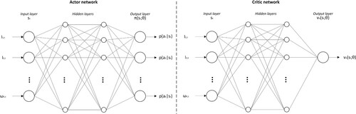
A high-level description of the PPO algorithm is shown in Algorithm 1. We use the actor-critic structure as described by Schulman et al. (2017). The policy is represented by a neural network with parameters θ, also known as the actor network $\pi (s_t;\theta )$. Another neural network with parameters ϕ is used to estimate the value function when following the policy of the actor, called the critic network $v^{\pi }(s_t;\varphi )$. The values of the parameters in the neural networks are updated by the algorithm while training. The updates from the old to the new policy are clipped, as this avoids large differences in the policy, and results in relatively stable training behaviour (Schulman et al. 2017). To provide samples to train the neural network, a buffer is filled with training data of states, actions, and rewards that are gotten when rolling out the current policy of the actor network. These training data are used to compute the loss functions required for updating the network weights. In applying this PPO algorithm, multiple updates are performed with the same training data.

In this paper, the ‘standard’ PPO algorithm as described by Schulman et al. (2017) was implemented, with several modifications to make it suitable for S-CLSP. The main modifications are using a feasibility mask, scaling the states and rewards, and using knowledge of the optimal solution for small problem instances to reduce the action space (Section 4.2).

4.1. Neural network architecture

Fully connected feed-forward neural networks are used (similar to the work by Schulman et al. 2017) consisting of two hidden layers with a width of 256 nodes, using a hyperbolic tangent (tanh) activation function. For problem instances with $|A_t|\ge 1000$, 2 hidden layers with a width of 512 nodes were used. The dimension of the first layer (i.e. input layer) is the same as the dimension of the state space ($2\cdot K$), and the dimension of the last layer in the actor network (i.e. output layer) is the same as the dimension of the action space ($|A_t|$). The critic network is set up in the same way as the actor network, except for the last layer, which just has one dimension and outputs an estimate of the value function. This architecture is illustrated in Figure 1.

Figure 1. Illustration of neural network architecture.

Figure showing the actor network on the left with a large output layer, and the critic network on the right with only a single output node. Both network have the same state nodes as input.

For initialising the neural network, the method described by Glorot and Bengio (2010) is used to initialise the parameters. Glorot-Uniform initialisation is used for the weights, and the bias is initialised at 0. This method is suggested by them to ensure that gradients can propagate well through the network and results in faster convergence.

4.2. Adjusting state and action spaces

To ensure that the neural network and its hyperbolic tangent activation function respond well to the state input, the values of our state space are scaled such that they are in the interval $[-1,1]:s_t^i=s_t/s_t^{lim}$. We set $I_{lim}^i$ at 15 times the average demand rate $d_i$ (11(11) $s_t^{lim}=(I_{lim}^1,I_{lim}^2,\dots ,I_{lim}^K,1,1,\dots ,1).$(11) ). When the optimal policy is found for small problem instances, it is unlikely to result in inventory levels that exceed this limit. Therefore, setting this limit is also a good way of narrowing down the potential state space, to ensure that the algorithm encounters primarily states that are reasonable in the exploration phase: (11) $s_t^{lim}=(I_{lim}^1,I_{lim}^2,\dots ,I_{lim}^K,1,1,\dots ,1).$(11) This inventory and backorder limit was also implemented in inventory transition function (12(12) $I_{i,t}=max(min(I_{i,t-1}+q_{i,t}-d_{i,t},I_{lim}^i),-0.5\cdot I_{lim}^i).$(12) ). Note that we expect less backorders than inventory, so the backorder limit is half of the inventory limit: (12) $I_{i,t}=max(min(I_{i,t-1}+q_{i,t}-d_{i,t},I_{lim}^i),-0.5\cdot I_{lim}^i).$(12) We apply the PPO algorithm with a discrete action space. This means that the actor can choose any action in the feasible set. The feasible set consists of all the feasible combinations of $q_t^i$, given the production capacity. This means that as the number of products or the capacity limit increases, the number of feasible combinations and thus the size of the action space increases dramatically, which comes with a decrease in algorithm performance and an increase in computational costs. For this reason, the problem was modelled with a batch size $b{s}_i$, which reduces the dimensions of the action space.

4.2.1. Action reduction

Even with the use of batch sizes in the model, the list of all feasible actions is still very large, while it is very unlikely that all of the actions will be desirable. Using knowledge about the characteristics of the optimal solution for small problem instances allows us to reduce the action space for larger instances. By solving the problem to optimality for three products, it was observed that typically not all products were produced in one period, even if the inventory levels were low. Additionally, the produced quantities were never larger than the EOQ values. Therefore, we only considered actions that had a maximum number of products ($K^{max}$) produced in one period, and the production quantity was not allowed to be greater than the number of batches required to produce the EOQ plus one batch of slack. The determination of $K^{max}$ and EOQ is described in the appendix.

4.2.2. Eligibility and feasibility masks

From the optimal solution, we know that in certain states, some actions will never be chosen (we call them ineligible), and some actions are infeasible due to set-up times. The PPO algorithm could benefit from avoiding to explore these actions, as they are not beneficial in achieving low costs. We hid those actions with an eligibility mask. To ensure that the policy consists of eligible actions (i.e. a probability distribution with zero probability for ineligible actions), the eligibility mask uses a soft-max activation function over the eligible actions. In the case that a product was not set up at the beginning of period t, and its inventory position $I_{i,t}$ was above a threshold $5\cdot {\mu }_i/I_{lim}^i$, that product would not be eligible for production in period t.

Moreover, given the set-up carryover variable ${\omega }_{i,t}$, some actions in $A_t$ could be infeasible due to the required set-up times. The determination of feasibility is made based on ${\omega }_{i,t}$ and $s{t}_i$, such that all actions satisfy capacity constraint (1(1) $\sum _{i=1}^K{q}_{i,t}+z_{i,t}\cdot s{t}_i\le CAP\mathrm{\forall }t\in \{1,\dots ,T\}.$(1) ). The feasibility masks work in the same way as the eligibility mask. This feasibility and eligibility mask is computed every time the MDP is in a new state, so this augmentation to the standard PPO algorithm comes at an additional computation cost (see Section 5.4).

4.3. Collecting training samples

In each training iteration, training data is collected by gathering a sample from the current policy of actor $\pi (s_t;\theta )$, starting in a state with no inventory and a random product set up. By following the current policy and drawing random demand, we generate this sample. This policy is simulated for a trajectory of $m_t=m+{\log }_{\gamma }\left(0.5\right)$ periods to approximate the infinite horizon MDP (Tang and Abbeel 2010) and the state, action and scaled reward are stored for each period in the (training) buffer. The rewards are normalised before use in further calculations to ensure that scale of the rewards is similar to that of the state input features, which secures that the difference in scale does not inhibit learning. Additionally, the probability distribution over all actions, made by $\pi (s_t;\theta )$, is stored for each state that is visited, as well as the value predictions of each visited state, made by $v^{\pi }(s_t;\varphi )$. For training the networks, a truncated buffer (m) of 256 periods of the trajectory is used.

4.4. Computing advantages

Before the weights can be updated, the advantage of taking a certain action rather than another needs to be calculated, such that the policy is updated in a direction that increases the chances of taking better actions. To do so, we use the generalised advantage estimation method (Schulman et al. 2016). This method is proposed as a way of estimating the gradient that significantly reduces variance and has a tolerable level of bias, increasing the effectiveness of learning with policy gradient techniques. Advantage function (13(13) $A^{\pi }(s,a)=Q^{\pi }(s,a)-V^{\pi }\left(s\right).$(13) ) measures whether or not an action $Q^{\pi }(s,a)$ performs better than the policy's default behaviour $V^{\pi }\left(s\right)$: (13) $A^{\pi }(s,a)=Q^{\pi }(s,a)-V^{\pi }\left(s\right).$(13) Generalised advantage estimator (14(14) $\begin{array}{rl}& {\hat{A}}_t^{GAE(\gamma ,\lambda )}=\sum _{l=0}^{m_t-t}(\gamma \lambda {)}^l{\delta }_{t+l}^V,\end{array}$(14) ) is the exponentially weighted average of the k-step estimators (15(15) $\begin{array}{rl}& {\hat{A}}_t^{\left(k\right)}=\sum _{l=0}^{k-1}{\gamma }^l{\delta }_{t+1}^V,\end{array}$(15) ) that estimate the advantage of the actions (16(16) $\begin{array}{rl}& {\delta }_t^V=r_t+\gamma V\left(s_{t+1}\right)-V\left(S_t\right).\end{array}$(16) ) for k-steps ahead, with decay parameter λ. The calculated advantages are normalised before being used for the updates: (14) $\begin{array}{rl}& {\hat{A}}_t^{GAE(\gamma ,\lambda )}=\sum _{l=0}^{m_t-t}(\gamma \lambda {)}^l{\delta }_{t+l}^V,\end{array}$(14) (15) $\begin{array}{rl}& {\hat{A}}_t^{\left(k\right)}=\sum _{l=0}^{k-1}{\gamma }^l{\delta }_{t+1}^V,\end{array}$(15) (16) $\begin{array}{rl}& {\delta }_t^V=r_t+\gamma V\left(s_{t+1}\right)-V\left(S_t\right).\end{array}$(16) We set γ and λ to the values that are found to work well in the PPO algorithm (Schulman et al. 2017): $\lambda =0.95$ and $\gamma =0.99$.

4.5. Updating the network weights

To update the weights of θ and ϕ, mini-batch gradient descent is applied, using the Adam optimiser (Kingma and Ba 2014) with learning rates $1e^{-4}$, which was found to work well (Schulman et al. 2017). With mini-batch gradient descent, the sample is split into batches, and an average gradient is calculated for each batch. A batch size of 64 is used, meaning that, with our truncated buffer size of 256, there are 4 batches. In addition, the training data is used 10 times (called epochs), meaning that in total the networks are updated 40 times in each training iteration. The data is shuffled in each batch to decorrelate the updates and avoid overfitting (Mnih et al. 2013).

For each update two loss functions are computed, $L_a$ for $\pi (s_t;\theta )$ and $L_c$ for $v^{\pi }(s_t;\varphi )$. For actor loss (17(17) $\begin{array}{rl}{L}_a\left(\theta \right)& ={\hat{\mathbb{E}}}_t[\mathrm{m}\mathrm{i}\mathrm{n}\left(r_t\right(\theta ){\hat{A}}_t,\mathrm{c}\mathrm{l}\mathrm{i}\mathrm{p}(r_t\left(\theta \right),1-ϵ,1+ϵ\left){\hat{A}}_t\right)\\ & +c_e\cdot S\phantom{\left(r_t\right(\theta ){\hat{A}}_t,\mathrm{c}\mathrm{l}\mathrm{i}\mathrm{p}(r_t\left(\theta \right),1-ϵ,1+ϵ\left){\hat{A}}_t\right)}],\end{array}$(17) ), the mean loss of all the sample points in the batch is used, based on the calculated advantages, as well as the ratio of the updated policy to the old policy. Buşoniu et al. (2018) mention that because of the non-linear nature of neural networks, a change to the policy ‘can quickly change the distribution of the state visited by the updated policy away from the on-policy distribution for which the update was valid’ (p. 20). Therefore, the changes in the policy distribution should be kept small, which in PPO is done by clipping the objective function (Schulman et al. 2017). The ratio of the updated policy to the old policy (18(18) $\begin{array}{rl}{r}_t\left(\theta \right)& =\frac{{\pi }_{\theta }\left(a_t|s_t\right)}{{\pi }_{{\theta }_{old}}\left(a_t|s_t\right)}.\end{array}$(18) ) is clipped to the range of $1\pm ϵ$ to ensure that the update to the policy network is not too large, which results in a more stable training behaviour: (17) $\begin{array}{rl}{L}_a\left(\theta \right)& ={\hat{\mathbb{E}}}_t[\mathrm{m}\mathrm{i}\mathrm{n}\left(r_t\right(\theta ){\hat{A}}_t,\mathrm{c}\mathrm{l}\mathrm{i}\mathrm{p}(r_t\left(\theta \right),1-ϵ,1+ϵ\left){\hat{A}}_t\right)\\ & +c_e\cdot S\phantom{\left(r_t\right(\theta ){\hat{A}}_t,\mathrm{c}\mathrm{l}\mathrm{i}\mathrm{p}(r_t\left(\theta \right),1-ϵ,1+ϵ\left){\hat{A}}_t\right)}],\end{array}$(17) (18) $\begin{array}{rl}{r}_t\left(\theta \right)& =\frac{{\pi }_{\theta }\left(a_t|s_t\right)}{{\pi }_{{\theta }_{old}}\left(a_t|s_t\right)}.\end{array}$(18) Typically as the training procedure progresses, the entropy of the policy decreases (i.e. the actions become less random). To encourage the exploration of actions, which is desirable in the case of having large action spaces, we add an entropy bonus to the policy loss function (Mnih et al. 2016). This entropy bonus is composed of an entropy coefficient $c_e$ multiplied with the average Shannon entropy S (1948) of an episode buffer.

The value loss is defined as the mean-squared error (19(19) $L_v\left(\varphi \right)={\left(v\right(s_t;\varphi )-C_t)}^2.$(19) ), where the predictions of the critic network are compared with the real observations of the cost $C_t$ for the sample point that occurred at time t: (19) $L_v\left(\varphi \right)={\left(v\right(s_t;\varphi )-C_t)}^2.$(19) $C_t$ is defined as the sum of the discounted costs until the end of the buffer trajectory and the discounted infinite horizon cost after the end of trajectory (20(20) $C_t=\sum _{t^{\mathrm{\prime }}=t}^{m_t}\left[{\gamma }^{t^{\mathrm{\prime }}-t}{c}_{t^{\mathrm{\prime }}}\right]+{\gamma }^{m_t-t}v(s_{m_t};\varphi ).$(20) ). Since the infinite horizon cost after the end of the trajectory is not known, this is approximated by the value function in the last period of the trajectory: (20) $C_t=\sum _{t^{\mathrm{\prime }}=t}^{m_t}\left[{\gamma }^{t^{\mathrm{\prime }}-t}{c}_{t^{\mathrm{\prime }}}\right]+{\gamma }^{m_t-t}v(s_{m_t};\varphi ).$(20) Considering that the actor and critic networks do not share weights, combining the policy and value loss is not necessary.

4.6. Training procedure

Every 100 iterations, we evaluate the performance of the current policy by simulating it n = 5 times for 1000 time periods, removing a warm-up period of length 10. Based on this, the 95% confidence interval of the mean costs per period is calculated (21(21) $CI=(\overline{x}-1.96\cdot \frac{\overline{\sigma }}{\sqrt{n}},\overline{x}+1.96\cdot \frac{\overline{\sigma }}{\sqrt{n}}).$(21) ), using the mean ($\overline{x}$) and the standard deviation ($\overline{\sigma }$) of the costs of the n replications: (21) $CI=(\overline{x}-1.96\cdot \frac{\overline{\sigma }}{\sqrt{n}},\overline{x}+1.96\cdot \frac{\overline{\sigma }}{\sqrt{n}}).$(21) To stop the training procedure, two criteria that indicate convergence have to be met. The first criterion is that the average performance in the evaluation periods has not improved (i.e. average performance does not exceed highest upper bound) for 10 consecutive evaluation periods. If the performance of the current policy is very unstable, the confidence interval (and thus upper bound) may become very wide. To avoid early stopping as a result of this wide interval, we clip the upper bound: $\overline{x}+min(0.025\cdot \overline{x},1.96\cdot \frac{\overline{\sigma }}{\sqrt{n}})$. The second criterion is that the entropy of the actor is low enough, meaning that the policy is not that random anymore. Even though the output of the actor is a stochastic policy, we know that the policy will converge to a somewhat deterministic policy. To ensure that the algorithm has arrived at a fairly deterministic policy, we consider that if the entropy is below 20% of the maximum entropy, the entropy is low enough. If these two criteria have not been met after 10,000 training iterations, the training procedure is stopped.

An overview of the PPO algorithm hyper-parameters used in the implementation can be found in Table 1. Experimentation on the hyper-parameters confirmed the suitability of the parameters found by Schulman et al. (2017).

Table 1. PPO hyperparameters.

Hyperparameter	Parameter value
γ	0.99
λ	0.95
Maximum number of iterations	10,000
Buffer size	256
Batch size	64
Update epochs	10
Layers	(256, 256) if $\left|A_t\right|<1000$
	(512, 512) if $\left|A_t\right|\ge 1000$
Activation function	tanh
Initialisation of weights	Glorot-Uniform
Entropy coefficient $c_e$	0.01
Learning rates Adam optimiser	$1e^{-4}$

5. Results

Experiments are carried out to examine the applicability of the PPO algorithm to the S-CLSP. The applicability consists of three elements: (1) performance, (2) scalability, and (3) explainability. Simulation studies are conducted with various problem settings to show the performance and scalability of the PPO algorithm. The performance of the learned inventory policy by the PPO algorithm is compared to the optimal policy (whenever possible) and a heuristic policy (Section 5.1). Throughout this section, we use the term ‘solution’ to represent the results of a policy in the simulation study.

To test the quality of the PPO algorithm, experiments are conducted with three different set of experiments. In each of these sets, we generate problem instances with different problem parameters (details of the set-up in Section 5.2, results in Section 5.3). The scalability of the PPO algorithm is studied by examining the relationship between the computation time and the problem size (Section 5.4). Finally, a multiple linear regression analysis is done to explore the PPO algorithm's explainability (Section 5.5).

5.1. Benchmark heuristic policy

To evaluate the performance of the PPO algorithm in larger problem settings, it must be compared to a benchmark. Unfortunately, no generic policy exists in the literature that incorporates both stochastic demand and a limited production capacity in an infinite horizon. In cases with unlimited capacity, the products are looked at in isolation. However, when there is limited production capacity available, the individual product replenishment decisions may conflict with each other, resulting in infeasible production schedules and excessive backorders. Therefore, some mechanism is needed to prioritise the different production decisions. When stochasticity is ignored in a capacitated system, a fixed replenishment cycle is used. In such a setting, inventory may deplete faster than expected due to demand uncertainty, also resulting in backorders. A more flexible mechanism is needed to react to demand realisations.

We present the aggregate modified base-stock heuristic (AMBS) as a way of dealing with stochastic demand and limited production capacity in an infinite horizon. It is a simulation-based heuristic, where we optimise the parameters for the backorder threshold ($B_{min}$), holding cost threshold ($H_{max}$) and set-up threshold ($Z_{max}$) using grid-search. In every period, the products are ranked in descending order of the expected backorder costs (given the current inventory levels). If this expected backorder cost is above some threshold $B_{min}$, a batch of this product is produced. This logic is continued until capacity runs out in a period, or if all products are below this threshold. In problem instances where we have a set-up time, there is an additional requirement that only $Z_{max}$ new set-ups are allowed in a period, which ensures that capacity is mainly used for production, rather than set-ups. If there is capacity left, and all products are below the backorder threshold, additional production batches are decided for the products that are set up in that period. The product that is produced last is determined based on the lowest inventory to EOQ ratio (as we make sure that we can continue producing this product in the next period). For the other products that are set up, we rank them in ascending order of their inventory level to the EOQ quantity ratio. If we can produce a batch of a product without exceeding the holding cost threshold $H_{max}$, we will produce this batch. This holding cost threshold ensures that the capacities are not exhausted as much as possible, as this could result in too much inventory build-up. Detailed notation can be found in the appendix.

Experimentation shows that our AMBS heuristic outperforms the lot size-reorder point policy $(Q,R)$ as presented by Nahmias and Olsen (2015b) by $\sim 16.5\mathrm{\%}$. This $(Q,R)$-policy is presented as optimal for a situation with stochastic demand and unlimited capacity under continuous review .¹ However, in case of limited capacity, deciding the production quantities on an aggregate level, taking into consideration the inventories of all the products, provides benefits. Furthermore, the AMBS heuristic performs only 10% worse than the optimal solution to a deterministic demand problem with limited production capacity (based on assumptions of having sequence-independent set-up times and a rotational cycle policy) as presented by Nahmias and Olsen (2015a). The average optimality gap between the AMBS heuristic and the optimal policy is 8.77% (more on the optimal policy in Section 5.3).

5.2. Experimental set-up

In the first set of experiments, problem instances were generated for each combination of the number of products (K), demand variability (COV) and capacity factor (cf), as shown in Table 2. Demand follows a discrete uniform distribution, similar to Vanvuchelen, Gijsbrechts, and Boute (2020). Following Tempelmeier (2011), we also investigate different levels of the coefficient of variation (COV). In settings with a high COV = 0.58, the demand follows the distribution $U\{0,8\}$, where a low COV = 0.14 has the distribution $U\{3,5\}$. We vary the capacity available for production based on parameters that Tempelmeier (2011) used for creating low (cf = 1.1) and medium (cf = 1.5) capacity scenarios. Based on the average demand ${\mu }_i$, batch sizes $b{s}_i$ and capacity factor cf, CAP for a problem instance is computed (22(22) $CAP=\lceil cf\cdot \sum _{i\in K}\frac{{\mu }_i}{b{s}_i}\rceil .$(22) ). All products in this set are identical in terms of demand distribution and cost settings. In this set, the backorder costs, set-up costs, batch sizes and set-up times are fixed as shown in Table 2. (22) $CAP=\lceil cf\cdot \sum _{i\in K}\frac{{\mu }_i}{b{s}_i}\rceil .$(22) In the second set of experiments, problem instances are generated for a combination of different numbers of products K, backorder costs $b_i$, set-up costs $k_i$, as well as for a heterogeneous set of products in terms of demand and cost settings. Details on the experiments with heterogeneous products are shown in Table 5. We base the settings for the backorder costs on the experiments by Tempelmeier (2011), who considers different fill rate (${\text{β}}_i$) constraints. Rather than a service level constraint, we determine costs for backorders such that the PPO algorithm takes this into consideration when learning to minimise the costs. In our problem statement, we consider a gamma service level (which also considers waiting time for backorders) rather than a fill rate (Tempelmeier 2006). We consider service level targets of 90% and 98%. To transform this target service level to backorder costs (23(23) $\begin{array}{rl}{\text{β}}_i& =\frac{b_i}{b_i+h_i},\end{array}$(23) ), we use the idea of the critical ratio of the newsvendor model (Arrow, Harris, and Marschak 1951) to determine the ratio of holding cost to backorder costs, where we have holding costs $h_i=1$ in all experiments. This results in $b_i=9$ for a low service target and $b_i=49$ for a high service target. Even though (23(23) $\begin{array}{rl}{\text{β}}_i& =\frac{b_i}{b_i+h_i},\end{array}$(23) ) is based on fill rate as a service measure, we also consider it appropriate for the gamma service level as our experiments show that the gamma service level (average 91.3% for set 1) and fill rate (average 92.8% for set 1) are very similar as ‘repeated’ backorders are unlikely. To determine the set-up costs, we use different values of $TB{O}_i$ of 5 and 10 periods (24(24) $\begin{array}{rl}{k}_i& =\frac{h_i\cdot TB{O}_i^2\cdot {\mu }_i}{2}.\end{array}$(24) ) as used by Tempelmeier (2011). When varying the demand of the products, we have half of the products with a low mean demand ${\mu }_i=2$ and the other half of the products have a high mean demand ${\mu }_i=4$. In this set, the coefficient of variation, capacity, batch sizes and set-up times are fixed. (23) $\begin{array}{rl}{\text{β}}_i& =\frac{b_i}{b_i+h_i},\end{array}$(23) (24) $\begin{array}{rl}{k}_i& =\frac{h_i\cdot TB{O}_i^2\cdot {\mu }_i}{2}.\end{array}$(24)

Table 2. Experimental settings.

Parameter	Set 1	Set 2	Set 3
Number of products, K	{2, 3, 4, 5, 6, 7, 8, 9, 10}	{4, 6, 8}	{4, 6, 8}
Coefficient of variation, COV	{0.14 (low), 0.58 (high)}	0.58	0.58
Capacity factor, cf	{1.1 (low), 1.5 (high)}	1.1	1.5
Mean demand, ${\mu }_i$	4 $\mathrm{\forall }i\in K$	{4 $\mathrm{\forall }i\in K$, {2,4} mixed{	4 $\mathrm{\forall }i\in K$
Backorder cost, $b_i$	9	{9, 49, mixed}	9
Time between orders, $TB{O}_i$	10	{5, 10, mixed}	{5, 10}
Set-up time factor, $s{f}_i$	0	0	{0.3, 0.5}
Batch size, $b{s}_i$	$\lfloor {\displaystyle \frac{K}{2}}\rfloor \cdot 2$	$\lfloor {\displaystyle \frac{K}{2}}\rfloor \cdot 2=4$	{1, 2, 4, 8, 10}
Number of experiments	36	54	52

In the last set of experiments, problem instances are generated for a combination of different numbers of products K, set-up costs $k_i$, set-up times $s{t}_i$ and batch sizes $b{s}_i$. The set-up costs are determined using the $TB{O}_i$ (24(24) $\begin{array}{rl}{k}_i& =\frac{h_i\cdot TB{O}_i^2\cdot {\mu }_i}{2}.\end{array}$(24) ). The set-up times are based on experiments run by Brandimarte (2006), who use a set-up time factor sf that indicates the fraction of capacity that would be lost if all products would be set up in one period. They use the factors 0.3 and 0.5, and we allocate this time required for set-ups evenly over all products (25(25) $s{t}_i=\frac{sf\cdot CAP}{K}.$(25) ). We varied the batch sizes from small ($b{s}_i=1$, i.e. no batch size) to large batch sizes ($b{s}_i=10$, 2.5 times the period demand). In this set, the coefficient of variation, capacity, the mean demand, and the backorder costs are fixed. (25) $s{t}_i=\frac{sf\cdot CAP}{K}.$(25)

Considering there is some randomness involved when training the neural networks using the PPO algorithm (e.g. initialising, filling the buffer, sampling from the buffer), we replicate the training in each experiment three times to analyse the robustness of the algorithm, setting a different random seed for each replication. This means we have three trained actor neural networks per experiment setting. The final performance of the PPO algorithm is determined by 10 simulation runs for 10,000 periods, where the first 1000 periods are discarded (warm-up periods). For each experiment setting, all three neural networks and the AMBS heuristic encounter the same demand realisations in the simulation runs. We report the best and average PPO solution for each experimental setting.

5.3. Experiment results

In this section, we discuss the results of the various set of experiments. We report the improvement compared to the AMBS heuristic in terms of costs. In the appendix, extended tables are presented that also show the difference to the AMBS heuristic for the average inventory levels, backorders, set-ups and lot sizes .²

Only the problem instances with K = 2 products were computationally tractable to solve to optimality .³ Value iteration, a type of Dynamic Programming was used to find the optimal solution. On average, a small optimality gap of 5.24% was found, and the gap is even smaller for the best-performing PPO replications. The gap was lower for low variability and medium capacity settings (see Table 3).

Table 3. Optimality gaps of best PPO performance (a) and average PPO performance (b) for K = 2 products in %.

COV	cf = 1.1	cf = 1.5	Avg
(a) Best PPO
Low	3.47	2.31	2.89
High	5.39	4.60	4.99
Avg.	4.43	3.45	3.94
(b) Average PPO
Low	4.44	5.07	4.75
High	6.33	5.14	5.73
Avg.	5.38	5.10	5.24

5.3.1. Set of Experiments 1

In Table 4, the differences between the AMBS heuristic and best PPO solution are shown for the first set of experiments. We observe that the PPO solution outperforms the benchmark on average with 7% lower costs, and even 8% when we look at the best performing replication. In situations with medium capacity and lower variability of demand, this improvement is larger. The main explanation for this improvement is a lower average inventory level and a lower number of set-ups required for the PPO solution, against an increase in the number of backorders, visualised in Figure 2. Because less set-ups are required, the lot sizes are larger as production occurs less frequently. The PPO algorithm specifically looks to find a balance between all different cost components, and it appears to work better at doing so than the AMBS heuristic. Interestingly, we find that the PPO algorithm results in an average gamma service level of 91.3%, which is close to the target of 90%, whereas the AMBS heuristic reaches 95.1%, exceeding the target considerably.

Figure 2. Illustration of (a) average product inventory costs, (b) average product backorder costs and (c) average product set-up costs for the PPO (best replication) and AMBS solutions.

Figure comparing the PPO and AMBS performance in experiment set 1.

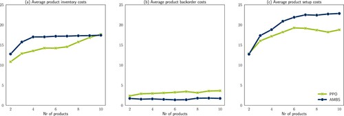
Table 4. Results for experiment set 1 showing the difference in average period costs between the best PPO performance (a), average PPO performance (b) and the AMBS heuristic in %. The size of the action space for the different problem instances is also shown (c).

(a) Best PPO
cf	COV	K = 2	K = 3	K = 4	K = 5	K = 6	K = 7	K = 8	K = 9	K = 10	Avg
1.1	Low	−4.23	−9.56	−11.61	−10.39	−9.14	−10.51	−10.49	−9.83	−7.72	−9.28
	High	0.71	−2.95	−7.22	−6.87	−6.25	−7.22	−7.37	−5.68	−2.17	−5.00
1.5	Low	−9.99	−12.35	−13.90	−13.10	−12.23	−12.82	−11.02	−9.04	−5.15	−11.06
	High	−3.05	−8.24	−7.77	−9.32	−9.37	−8.46	−8.81	−6.27	−3.28	−7.17
Avg		−4.14	−8.27	−10.12	−9.92	−9.24	−9.75	−9.42	−7.70	−4.58	−8.13
(b) Average PPO
cf	COV	K = 2	K = 3	K = 4	K = 5	K = 6	K = 7	K = 8	K = 9	K = 10	Avg
1.1	Low	−3.34	−9.02	−10.74	−9.19	−8.96	−9.12	−9.59	−6.83	−5.78	−8.06
	High	1.61	5.92	−6.04	−6.55	−5.77	−6.72	−5.21	−3.68	−0.09	−2.95
1.5	Low	−7.57	−11.48	−13.03	−12.13	−11.44	−11.64	−9.99	−8.38	−3.94	−9.96
	High	−2.55	−7.16	−7.63	−8.94	−9.10	−8.08	−7.56	−5.08	−2.14	−6.47
Avg.		−2.96	−5.43	−9.36	−9.20	−8.82	−8.89	−8.09	−5.99	−2.99	−6.86
(c) Size of action space $A_t$
1.1		21	85	81	181	381	1058	881	2275	2751	857
1.5		28	136	115	321	662	1716	1589	3751	6276	1622

Table 5. Experimental settings set 2 and results showing the difference in average period costs between the best PPO replication (a) and average of the PPO replications (b) and the AMBS heuristic in %.

	(a) Best PPO			(b) Average PPO
Setting	K = 4	K = 6	K = 8	K = 4	K = 6	K = 8
Homogeneous products: identical demand levels and costs
1. Low $b_i$ and low $TB{O}_i$	−3.19	−1.34	0.61	−2.78	0.05	2.42
2. Low $b_i$ and high $TB{O}_i$	−6.06	−6.29	−7.44	−5.52	−5.75	−5.20
3. High $b_i$ and low $TB{O}_i$	1.58	7.19	8.03	2.33	8.71	9.98
4. High $b_i$ and high $TB{O}_i$	−1.44	−2.36	−2.11	−0.69	−1.04	−0.66
Heterogeneous products: identical demand levels but different costs
5. Low $b_i$, mixed $TB{O}_i$	−6.92	−5.41	−1.64	−5.95	−4.89	−0.96
6. Mixed $b_i$. low $TB{O}_i$	−0.78	1.51	3.66	0.83	2.12	4.93
7. Mixed $b_i$, high $TB{O}_i$	−4.02	−4.94	−5.14	−3.17	−4.07	−4.18
8. Mixed; low $b_i$ with low $TB{O}_i$ & high $b_i$ with high $TB{O}_i$	−3.94	−4.22	0.54	−3.67	−2.96	2.85
9. Mixed; low $b_i$ with high $TB{O}_i$ & high $b_i$ with low $TB{O}_i$	−3.28	−2.63	0.52	−3.05	−1.54	1.52
10. Mixed; all combinations	−5.46	−2.83	1.91	−4.56	−2.09	2.16
11. High $b_i$, mixed $TB{O}_i$	−1.73	0.71	4.03	−0.84	1.12	5.94
Heterogeneous products: different demand levels but identical costs
12. Low $b_i$ and low $TB{O}_i$	−5.60	−3.48	1.74	−4.82	−2.34	3.33
13. Low $b_i$ and high $TB{O}_i$	−10.24	−10.30	−7.29	−10.08	−9.93	−6.51
14. High $b_i$ and low $TB{O}_i$	0.19	2.24	7.91	0.82	3.42	8.15
15. High $b_i$ and high $TB{O}_i$	−4.44	−4.47	−2.47	−3.13	−3.43	−2.31
Heterogeneous products: different demand levels and costs
16. Low demand with low $b_i$ and low $TB{O}_i$ and vice versa	−11.89	−8.19	−4.35	−10.88	−6.90	−4.09
17. Low demand with high $b_i$ and high $TB{O}_i$ and vice versa	−2.29	−2.92	1.34	−2.04	−2.34	2.12
18. Mixed	−9.57	−4.79	−1.76	−8.55	−4.50	−1.54
Average difference	−4.39	−2.92	−0.11	−3.65	−2.02	1.00

From Table 4, we also see that there is a relationship between the size of the action space and the improvement found by the PPO solution. For larger action spaces, the gap with the benchmark starts to decrease. The PPO algorithm is based on exploring the different states and action spaces. When the action space is too large, sufficient exploration becomes more challenging, resulting in lower performance.

5.3.1.1 Impact of state and action space modifications

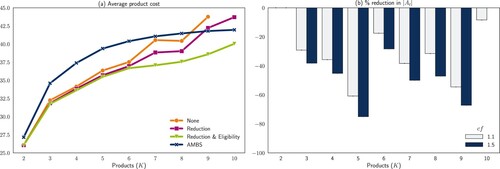
In our application of the PPO algorithm, we dealt with the large action space by applying knowledge about the characteristics of the optimal solution of small problem instances to model a ‘smart’ action space (as explained in Section 4.2), as well as adapting the size of the neural networks. Figure 3 shows the impact of the action reduction (Section 4.2.1) and eligibility masks (Section 4.2.2). Note that in the instance with K = 10 and cf = 1.5, the PPO algorithm without modifications was not able to run as the necessary neural network exceeded the computer memory size. As a result, these observations are missing from Figure 3. Observe that both the action reduction and eligibility mask modifications of the PPO algorithm were necessary to enable it to outperform the AMBS heuristic in larger problem instances. Figure 3 also indicates that using some knowledge about the characteristics of the optimal solution of small problem instances substantially reduces the action space. However, this modification alone is not enough to improve the performance of the PPO algorithm. This combination of action reduction and eligibility masks is needed to avoid the algorithm getting stuck in parts of the action space that will not provide good solutions. Nevertheless, the eligibility mask modifications come at an additional computation cost (Section 5.4).

Figure 3. The impact of state and action space modifications on (a) the average product costs in the best PPO replications and (b) the size of the action space.

Figure showing impact of state and action space modification on costs and action space.

We suggest future research to investigate more methods to cope with large action spaces, such as initialising the PPO algorithm with a smart policy, changing some PPO algorithm parameters based on the size of the problem, encouraging more exploration in training the network, modelling the actions in a continuous space rather than discrete, or using an action elimination framework (Zahavy et al. 2018).

5.3.2. Set of Experiments 2

In Table 5, the differences between the AMBS heuristic and best and average PPO solution are shown for the second set of experiments. We observe that on average the PPO solutions outperform the benchmark with 3.65% for situations with four products. Similar to experiment set 1, we see the performance of the PPO algorithm decreasing as the number of products (and thus action space) increases. Especially in settings with a high $TB{O}_i$, the PPO solution performs better. The AMBS heuristic is mainly focused on producing a product when it exceeds some backorder cost threshold, while the PPO solution considers the total costs. Also for problem instances with heterogeneous products (in terms of costs and demand levels), PPO outperforms the AMBS. The AMBS does consider the item-specific backorder costs, but then does not consider the item-specific set-up costs in the decision to start production. Furthermore, we find that in experiments with heterogeneous products in terms of costs, related to having product-specific service level targets, the PPO algorithm is better at reaching differentiated service level targets and prioritising the high-service products than the AMBS heuristic. In situations with low $TB{O}_i$ and high $b_i$, the AMBS heuristic performs slightly better than PPO. Generally, PPO results in lower inventory and higher backorders than AMBS, meaning that higher $b_i$ leads to worse results. We suspect that this is a result of the fact that backorders are occurring much less frequently than the set-ups. The PPO algorithm learns a lot from all the events that are encountered, and if backorders are underrepresented in the events, this could inhibit the impact the PPO algorithm attributes to having backorders. Future research could focus on how to improve the ability to learn from rare events, for instance, by increasing their occurrence during the training iterations.

5.3.3. Set of Experiments 3

In Table 6, the differences between the AMBS heuristic and best PPO solution are shown for the third set of experiments. Here we see again the impact of the large action spaces on the performance of the PPO algorithm. Specifically, we see that for situations with 6 and 8 products, a minimum batch size is needed to start training, as otherwise the action space would be infeasible in terms of memory size. Nevertheless, the PPO algorithm generally manages to outperform the AMBS heuristic, with bigger improvements in the case of a high $TB{O}_i$. With a low $TB{O}_i$, the PPO algorithm requires less set-ups, resulting in lower costs. With a high $TB{O}_i$, the PPO solution has a sharp decrease in inventory and set-ups, resulting in higher backorders. Nevertheless, overall the PPO solution still finds lower costs than AMBS.⁴

Table 6. Results for experiment set 3 showing the difference in average period costs between the best (a) and average (b) PPO performance and the AMBS heuristic in %. The size of the action space (c) for the different problem instances is also shown.

			(a) Best PPO		(b) Average PPO		(c) Size of action space $A_t$
K	sf	$b{s}_i$	$TB{O}_i=5$	$TB{O}_i=10$	$TB{O}_i=5$	$TB{O}_i=10$	$TB{O}_i=5$	$TB{O}_i=10$
4	0.3	1	4.52	2.00	5.09	4.15	6031	1483
		2	−1.11	−3.04	−0.72	−1.55	855	379
		4	−2.39	−2.43	−1.42	−1.83	125	85
		6	−1.57	−5.24	−0.54	−4.58	39	35
		8	−80.83*	−8.40	−80.70*	−8.03	19	19
		10	−4.18	−5.87	−3.84	−4.76	19	19
	0.5	1	2.33	0.99	6.65	1.35	4609	1357
		2	0.83	−2.27	1.24	−1.78	651	319
		4	−1.89	−5.72	−1.33	−4.49	101	85
		6	−2.01	−5.28	−1.19	−4.58	39	35
		8	−88.69*	−8.45	−88.61*	−8.10	19	19
		10	−4.33	−5.87	−3.88	−4.84	19	19
6	0.3	4	5.77	−0.94	6.19	0.22	2072	1595
		6	1.61	−0.31	2.45	0.09	456	387
		8	−0.71	−4.09	0.36	−3.71	210	201
		10	1.08	−4.87	1.97	−4.60	84	90
	0.5	4	6.62	1.20	7.47	1.58	1352	1175
		6	2.24	−1.27	2.83	−0.15	396	387
		8	−0.60	−4.57	0.59	−2.16	195	201
		10	1.14	−4.94	2.04	−4.58	84	90
8	0.3	6	3.48	2.44	4.66	4.31	4983	2613
		8	4.09	1.34	5.17	3.04	1223	889
		10	2.53	−1.42	3.62	0.38	487	433
	0.5	6	5.55	2.63	6.32	3.92	3583	2613
		8	5.32	−1.25	5.86	0.19	943	889
		10	2.05	−1.36	2.26	0.40	487	433
Avg.			1.27	−2.58	2.16	−1.54	808	440

Notes: Starred figures (the outlier cases) are excluded from average calculations because they would skew the conclusion. For $K=\{6,8\}$ small batch sizes result in neural networks that exceed the memory size available, so there are no results in these cases.

The batch size was mainly implemented to effectively reduce the size of the action space. We observe that this measure was an effective way of finding improvements on the AMBS heuristic. Additionally, we see no increase in average cost for the PPO algorithm due to the reduced granularity in the action space with these current settings. One would expect that this batch size implementation would only decrease the performance of the AMBS heuristic, because for the heuristic a batch size is not necessary. Nevertheless, we found that even for the AMBS heuristic, a batch size of size 2 (costs: 115.00) or 4 (costs: 114.88) performs slightly better than no batch size (costs: 115.45). Even though the inventory increases somewhat, this is offset by a reduced number of backorders. However, for the AMBS heuristic, the large batch size showed to be ineffective in finding the right policy. With an increase in the batch size, the number of batches that can be produced in a period decreases dramatically (given the utilisation rate constraint). With a large batch size, the problem essentially changes from determining the best production quantity to a choice of allocating the scarce batch production slots to the different products. Therefore, we consider the implementation of the batch size effective, but note that the reduction in granularity should be reasonable.

5.4. Computation times

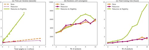
The total training time of the PPO algorithm is composed of the number of iterations required to converge during training, as well as the time needed to compute one iteration. Figure 4 shows the results of these components, as well as the impact of the state and action space modifications that were implemented in the PPO algorithm. The experiments are run on an Intel Xeon Gold 6130 Processor with 16 cores.

Figure 4. Illustration of (a) time per iteration in seconds, based on the weights of the actor and critic network, (b) the average number of iterations needed to converge in the PPO algorithm, based on the number of products in the experiment and demand variability and (c) the total training time until convergence in hours.

Illustration of computation times of the PPO algorithm.

Our analysis showed that the time required for one iteration is mainly based on the number of weights in the actor and critic networks for a problem instance. In one training iteration, the training buffer is filled, the advantage and gradient are computed and the network weights are updated. The number of weights in the actor network is dependent on the input vector (state space $2\cdot K$), number and size of hidden layers ($L^{size}$) and the output vector (action space $|A_t|$) (26(26) $\begin{array}{rl}{W}_{\theta }& =2\cdot K\cdot L^{size}+L^{size}\cdot L^{size}\\ & +L^{size}\cdot |A_t|+2\cdot L^{size}+|A_t|,\end{array}$(26) ). The number of weights in the critic network is computed in a similar way, but has only one output node (27(27) $\begin{array}{rl}{W}_{\varphi }& =2\cdot K\cdot L^{size}+L^{size}\cdot L^{size}\\ & +L^{size}\cdot 1+2\cdot L^{size}+1.\end{array}$(27) ): (26) $\begin{array}{rl}{W}_{\theta }& =2\cdot K\cdot L^{size}+L^{size}\cdot L^{size}\\ & +L^{size}\cdot |A_t|+2\cdot L^{size}+|A_t|,\end{array}$(26) (27) $\begin{array}{rl}{W}_{\varphi }& =2\cdot K\cdot L^{size}+L^{size}\cdot L^{size}\\ & +L^{size}\cdot 1+2\cdot L^{size}+1.\end{array}$(27) There appears to be linear growth in computation time as the number of weights grows. Note that we increased the size of the hidden layers for larger problems to accommodate the larger action space. This has a major impact on the number of weights and therefore computation time. Furthermore, the additional computations required for computing the eligibility mask in each new state impact the time per iteration significantly.

When investigating the average number of iterations required for convergence, the results of Set 1 give the most insights, as this number of iterations is mostly related to the variability of demand and the number of products. PPO is able to learn a good policy that improves on the benchmark quite quickly, but then slowly finds further improvements, until it converges (seen in Figure 5). In settings with higher variability, PPO requires on average 16% fewer iterations to converge to a solution. The reason for this might be that with high variability, the PPO algorithm will encounter a wider selection of the state-action space more quickly during training, and hence learn faster. Additionally, with an increasing number of products, PPO needs more iterations to converge, as was to be expected due to the increasing action space requiring more exploration.

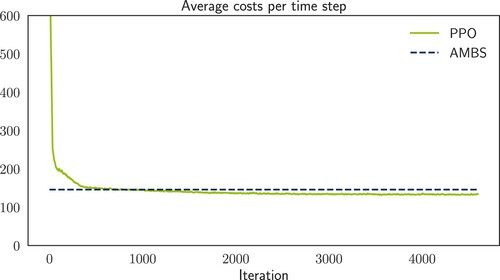
Figure 5. Performance of the PPO algorithm in experiment set 1 with K = 4, $COV=$ low and cf = 1.1. The AMBS performance is equalled after ∼1000 iterations, and PPO stops improving after ∼3500 iterations.

Figure showing how fast the PPO algorithm outperforms the AMBS heuristic.

Upon combining the time per iteration and the number of iterations, we see that more time is required to train larger problem instances. Additionally, we have performed three replications for each experiment setting to assess the robustness in learning, which requires three times the computation time. There is a slight gap in performance between the best and average replication, so a trade-off must be made for how much additional replications are desired to achieve small improvements in algorithm performance. However, it is good to note that this training can be done offline, and after the training, a steady-state policy results that can make decisions instantly based on the state variable. This is unlike MILP problems which have to be solved in their entirety at the moment of requiring a decision.

The time required for the AMBS heuristic to find the right $B_{min}$, $H_{max}$ and $Z_{max}$ parameters depends on the granularity of the grid search and the number of products (as this impacts the number of available batches). One parameter simulation requires $1.5\cdot \mathrm{K}$ seconds. In our grid search, we searched $66\cdot (K-1)$ combinations of parameters, meaning that for problems with 10 products, it took around 2.5 hours to find the optimal settings. Many actions could be taken to improve this computation time for AMBS, for instance, parallel search or a smarter grid search. The same holds for the PPO algorithm, as it is well known that neural network computations can be speed up significantly when run on GPU cores (as opposed to the CPU cores we used). While improvements are possible in the computation times, we demonstrate that the PPO algorithm performs well and also appears to scale linearly with regards to the size of the problem with our action space modifications to improve scalability. This shows that PPO is an interesting method for solving sequential decision-making problems with complicated real-life constraints.

5.5. Explainability

The use of neural networks often receives criticism that it is a ‘black box’ because it is hard to understand why a certain output is generated by the network (Heuillet, Couthouis, and Díaz-Rodríguez 2021). In this section, we make the output of the PPO networks interpretable. More specifically, we find a relationship between the action and the states in each of the experimental settings. For this explainability analysis, multiple regression analysis is employed to determine the relationship between the dependent variable (action) and multiple independent variables (states).

We define multiple linear regression equation (28(28) $q_{i,t}=c+{\text{β}}_1{I}_{i,t}+{\text{β}}_2\sum _{i\in K}{I}_{i,t}+{\text{β}}_3{\omega }_{i,t}.$(28) ), where for each product we predict the production quantity $q_{i,t}$ based on the product's inventory position $I_{i,t}$, the sum of all inventory positions in the system $\sum _{i\in K}{I}_{i,t}$ and the set-up carryover variable ${\omega }_{i,t}$: (28) $q_{i,t}=c+{\text{β}}_1{I}_{i,t}+{\text{β}}_2\sum _{i\in K}{I}_{i,t}+{\text{β}}_3{\omega }_{i,t}.$(28) For every problem instance in our experiment sets, Ordinary Least Squares estimation is used to estimate the intercept c and β coefficients for all products. The state variables explain a large part of the variance in the production quantity (average $R^2$-value = 0.621), and 97.4% of the β-coefficients were found to be statistically significant (p<.001 ).

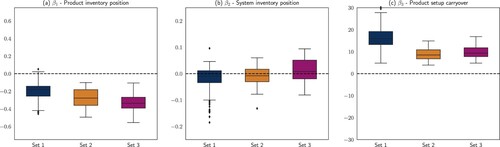
In Figure 6, the average value of the coefficients in each of the experiment sets is shown. We see that ${\text{β}}_1$ is typically negative, which means that when $I_{i,t}$ is higher, $q_{i,t}$ will be lower. This is as expected, because with high levels of inventory, less additional production is needed to prevent backorders. For ${\text{β}}_2$, which determines the relationship between the total system inventory position and $q_{i,t}$, we do not observe the same consistency in the direction of the coefficient. For ${\text{β}}_3$ large positive coefficients are observed, so ${\omega }_{i,t}$ seems to have the strongest relationships with $q_{i,t}$, indicating that when the machine is set up for product i, $q_{i,t}$ will be higher. When the demand uncertainty increases, the relationship between ${\omega }_{i,t}$ and $q_{i,t}$ becomes weaker. This can be explained by the fact that with more uncertain demand, switching production to another product to avoid backorders may be more beneficial than when the upcoming demand is fairly certain. For settings where the set-up costs are higher, ${\omega }_{i,t}$ has more impact on $q_{i,t}$, and $I_{i,t}$ becomes less important as a predictor. This indicates that when the set-up costs are high, it is better to take more advantage of the set-up by producing more of that product. This is consistent with expectations because when set-up costs are higher, it is sensible to try to prevent changing over to a new product due to the high costs.

Figure 6. Values of the coefficients in the regression models of the different experiment sets. $I_{i,t}$ and ${\omega }_{i,t}$ have the strongest relationship with $q_{i,t}$.

Figure showing boxplots of the values of the coefficients in the regression models, explaining the relationship between state and action variables.

Performing the multiple regression analysis shows that finding explanations for decisions made by the PPO solution can be done in a rather straightforward way. This is essential in enabling the understanding and trustworthiness of the algorithm, making it more suitable to use in practice. For future research, we suggest to look at more intricate explanation mechanisms as summarised by Heuillet, Couthouis, and Díaz-Rodríguez (2021) that may be better suited to the non-linear nature of neural networks, and that even have the capability to predict single policy actions (rather than general policy characteristics). Another avenue for future research is to utilise the findings of DRL algorithms to create new well-performing heuristics for complex problems that can be more easily understood and implemented in practice.

6. Conclusion

We investigated the applicability of a DRL methodology for finding near-optimal policies in the S-CLSP that minimise the costs of set-ups, backorders, and holding inventory. This shows how uncertainty in problems can be handled in optimisation, and how trade-offs can be found for conflicting objectives. Our study proposes to use the PPO algorithm, a method that performs well without extensive hyper-parameter tuning. We report that the PPO algorithm comes close to the optimal solution. In the experiments, we looked at various problem instances with different numbers of products, demand variability, capacity restrictions, cost settings, heterogeneous products (in terms of demand and costs) and set-up times. To demonstrate the potential of PPO in industrial use, we show that for larger problem instances where the optimal solution is unknown, the algorithm finds solutions that outperform the benchmark (an aggregate modified base-stock heuristic) by ∼7%.

In addition to the good performance of the algorithm, the computation time is promising as well. The computation time appears to have linear growth, making it an attractive method for solving industrial-size problems. An interesting avenue for future research is how to deal with larger action spaces, as we observe that the size of the action space may become restrictive in finding well-performing solutions. Moreover, we illustrate a way of explaining the resulting policies, which is an essential step in providing trust in the algorithm and enabling its implementation in the industry.

For future research, it is interesting to investigate how the algorithm could benefit from incorporating more information (e.g. demand forecasts) in the state space. Especially in the data-rich heavily interconnected supply network, this could be very advantageous. Other extensions could be to include additional objectives in the problem, such as reducing nervousness in production planning and investigating alternative explanation mechanisms for the outcomes of the algorithm. Implementation of this algorithm can support companies to reap the benefits of the digital supply chain, which include reducing costs and improving service to customers.

Acknowledgements

We thank SURFsara (www.surf.nl) for the support in using the Lisa Compute Cluster. We thank presenters in the Eindhoven seminar on RL for presentations and inspiration, and Wouter Kool for his feedback and insights on implementing RL.

Disclosure statement

No potential conflict of interest was reported by the author(s).

Data availability statement

The data that support the findings of this study are available from the corresponding author upon reasonable request.

Additional information

Notes on contributors

Lotte van Hezewijk

Lotte van Hezewijk is a Ph.D. candidate in the Department of Industrial Engineering & Innovation Sciences (IE&IS) at Eindhoven University of Technology (TU/e). Simultaneously, she works as Analytics Consultant at ORTEC. Her research is focused on exploring the benefits of Machine Learning in supply chain applications.

Nico Dellaert

Nico Dellaert is Associate Professor and Chair of Quantitative Analysis of Stochastic Models for Logistic Design in the Department of IE&IS at the TU/e. His prime research interests are on the integration of capacity and production decisions, on city logistics and multimodal transportation and on healthcare planning. In his work, he uses a large variety of mathematical modelling techniques. In most cases, companies or hospitals have been involved in the research.

Tom Van Woensel

Tom Van Woensel is Full Professor of Freight Transport and Logistics in the OPAC group (Operations, Planning, Accounting and Control) of the Department of IE&IS at the TU/e. Current interests include Last Mile Logistics, vehicle routing problems, crowd shipping, (service) network design, machine learning, Big Data, and IoT-driven issues and opportunities. He is also a director of the European Supply Chain Forum, in which some 75 multinational companies are involved.

Noud Gademann

Noud Gademann is Principal Consultant in Supply Chain Optimization at ORTEC. He also filled positions as assistant professor and researcher at the University of Twente and Eindhoven University of Technology in the field of Production and Operations Management and Warehouse Management, with a strong focus on the development and application of optimisation models and algorithms. He has a broad interest and experience in a large variety of industries, including discrete manufacturing, process industry, consumer goods and retail, warehousing and logistics, service industry, and rail services.

Notes

1 Since in our problem setting, demand events only occur once a day, this periodic review setting is similar to the continuous review problem.

2 For the lot size, we take the sum of production batches produced in subsequent periods that a product is continually set up

3 In Section 4.2, a problem with three products was solved to optimality. Nevertheless, to make this computationally tractable, the state space had to be made very small by adjusting the inventory limits. This is an arbitrary change that impacts the final solution, which we wanted to avoid in remaining experiments.

4 There are two outlier cases in the analysis, for which we notice extensive backorder build-up in the AMBS heuristic. In these situations with a very limited capacity of only 3 batches, the AMBS heuristic easily gets into a long 100% utilisation loop in which we produce 2 batches of different products in every period, without having the minimum required batch size for stability and recovering from backorder build-up. In these settings, the PPO algorithm learns to avoid such extensive backorder situations.

Appendices

Appendix 1. Action elimination

EOQ quantity (A1(A1) $Q_i^{EOQ}=\sqrt{\frac{2\cdot {\mu }_i\cdot k_i}{h_i}}.$(A1) ) is used to determine the maximum number of batches that are allowed to be produced for one product in one period. Note that in our problem instances with a limited amount of products, the capacity available for production is rarely enough to produce the EOQ quantity in one period. When the number of products increases, it could be that there is enough capacity to produce the EOQ quantity in one period, however, in these cases it is very uncommon that only one product is produced. Therefore, we do not expect this reduction technique to negatively impact the performance of the policy: (A1) $Q_i^{EOQ}=\sqrt{\frac{2\cdot {\mu }_i\cdot k_i}{h_i}}.$(A1) We determine a maximum number of products $K_{max}$ that is allowed to be produced in one period. We base this value on the probability that k products are produced in the same period. The probability $p_{1,i}$ that a product i is produced depends on the time between orders $TB{O}_i$ (A2(A2) $\begin{array}{rl}& p_{1,i}=\frac{1}{TB{O}_i},\end{array}$(A2) ) and (A3(A3) $\begin{array}{rl}& p_{0,i}=1-p_{1,i}.\end{array}$(A3) ): (A2) $\begin{array}{rl}& p_{1,i}=\frac{1}{TB{O}_i},\end{array}$(A2) (A3) $\begin{array}{rl}& p_{0,i}=1-p_{1,i}.\end{array}$(A3) To determine the probability that k products are produced in a period, we first compute the potential number of combinations of k products in the total set K. We then multiply this with the probabilities of production for each product (A4(A4) $P(X=k)=\frac{K!(K-k)!}{k!}\cdot p_1^k\cdot p_0^{(K-k)}.$(A4) ). $K_{max}$ is the maximum k for which $P(X=k)>0.01$, in other words, the maximum number of products which has a higher than 1% chance of being produced: (A4) $P(X=k)=\frac{K!(K-k)!}{k!}\cdot p_1^k\cdot p_0^{(K-k)}.$(A4)

Appendix 2. Aggregated modified base-stock heuristic

In this section, the detailed notation for the aggregate modified base-stock heuristic (Algorithm 2) is presented.

The heuristic bases its replenishment decisions partly on the expected backorder costs (A5(A5) $E\left[B{O}_{i,t}\right]=\{\begin{array}{ll}{\displaystyle b_i\cdot \sum _{x=I_{i,t}+1}^{d_{i,b}}\frac{x-I_{i,t}}{d_{i,b}-d_{i,a}}}& \text{if }{I}_{i,t}<d_{i,b},\\ 0& \mathrm{e}\mathrm{l}\mathrm{s}\mathrm{e}.\end{array}$(A5) ). This computation is based on the uniform demand distribution that is considered, denoted by $d_i\sim U\{d_{i,a},d_{i,b}\}$, with mean demand ${\mu }_i$: (A5) $E\left[B{O}_{i,t}\right]=\{\begin{array}{ll}{\displaystyle b_i\cdot \sum _{x=I_{i,t}+1}^{d_{i,b}}\frac{x-I_{i,t}}{d_{i,b}-d_{i,a}}}& \text{if }{I}_{i,t}<d_{i,b},\\ 0& \mathrm{e}\mathrm{l}\mathrm{s}\mathrm{e}.\end{array}$(A5) After the production batches have been decided to cover the expected backorders, additional production is determined for products that are set up. This determination is based on the order of the inventory to EOQ-value ratio (A6(A6) $I{L}_{i,t}^{EOQ}=\frac{I_{i,t}+b{s}_i\cdot q_{i,t}}{Q_i^{EOQ}}.$(A6) ) and (A1(A1) $Q_i^{EOQ}=\sqrt{\frac{2\cdot {\mu }_i\cdot k_i}{h_i}}.$(A1) ): (A6) $I{L}_{i,t}^{EOQ}=\frac{I_{i,t}+b{s}_i\cdot q_{i,t}}{Q_i^{EOQ}}.$(A6) After each decision on a production batch, the remaining capacity is computed (A7(A7) $CA{P}_{remaining,t}=CAP-\sum _{i\in K_{prod}\setminus i_{SU}}s{t}_i-\sum _{i\in K}{q}_{i,t}.$(A7) ), based on set-ups required and the number of batches produced: (A7) $CA{P}_{remaining,t}=CAP-\sum _{i\in K_{prod}\setminus i_{SU}}s{t}_i-\sum _{i\in K}{q}_{i,t}.$(A7) The relevant parameters in this problem are $B_{min}$, $H_{max}$ and $Z_{max}$. A grid-search is performed to find the best functioning values. The grid search is done by rolling out the heuristic 10 times for 1000 periods and discarding the first 100 as warm-up periods. The average costs are recorded, and the parameter combination of $B_{min}$, $H_{max}$ and $Z_{max}$ resulting in the minimum costs is used. For $B_{min}$ we look at several proportions of average EOQ-cost (A8(A8) $\begin{array}{rl}{C}_i^{EOQ}& =k_i\cdot \frac{{\mu }_i}{Q_i^{EOQ}}+h_i\cdot \frac{Q_i^{EOQ}}{2},\end{array}$(A8) ). In this case, $x_b\in \{0,0.1,0.2,\dots ,1.0\}$ (A9(A9) $\begin{array}{rl}{B}_{min}& =x_b\cdot \frac{\sum _{i\in K}{C}_i^{EOQ}}{K}.\end{array}$(A9) ): (A8) $\begin{array}{rl}{C}_i^{EOQ}& =k_i\cdot \frac{{\mu }_i}{Q_i^{EOQ}}+h_i\cdot \frac{Q_i^{EOQ}}{2},\end{array}$(A8) (A9) $\begin{array}{rl}{B}_{min}& =x_b\cdot \frac{\sum _{i\in K}{C}_i^{EOQ}}{K}.\end{array}$(A9) For $H_{max}$, we look at several proportions of the total EOQ holding costs. In this case, $x_h\in \{0.5,0.6,\dots ,1.0\}$ (A10(A10) $H_{max}=x_h\cdot \sum _{i\in K}(h_i\cdot Q_i^{EOQ}).$(A10) ): (A10) $H_{max}=x_h\cdot \sum _{i\in K}(h_i\cdot Q_i^{EOQ}).$(A10) For $Z_{max}$, we look at all possible quantities, given the number of products in the system. Since set-ups are carried over from one period to the next, there will be at most K−1 set-ups in a period. In this case, $x_z\in \{1,2,\dots ,K-1\}$.

Appendix 3. Extended experimental results

In this section, three tables are shown with the extended results for the experiment sets. They show the average costs of the PPO solution, as well as the differences in percentage in costs, inventory, backorders, set-ups and lot sizes, compared with the AMBS heuristic.

Table D1. Extended results for experiment set 1 showing the average PPO costs ($C_{PPO}$), difference in average period costs ($\mathrm{\Delta }{C}_t$), average inventory level ($\mathrm{\Delta }{I}_t^{+}$), average backorders ($\mathrm{\Delta }{I}_t^{-}$), average set-ups ($\mathrm{\Delta }{z}_t$) and average lot size ($\mathrm{\Delta }{q}_{i,t}\cdot b{s}_i$) between the best PPO performance and the AMBS heuristic in %.

		Low COV						High COV
K	cf	$C_{PPO}$	$\mathrm{\Delta }{C}_t$	$\mathrm{\Delta }{I}_t^{+}$	$\mathrm{\Delta }{I}_t^{-}$	$\mathrm{\Delta }{z}_t$	$\mathrm{\Delta }{q}_{i,t}\cdot b{s}_i$	$C_{PPO}$	$\mathrm{\Delta }{C}_t$	$\mathrm{\Delta }{I}_t^{+}$	$\mathrm{\Delta }{I}_t^{-}$	$\mathrm{\Delta }{z}_t$	$\mathrm{\Delta }{q}_{i,t}\cdot b{s}_i$
2	1.1	51.04	−4.23	−13.76	34.63	1.54	−1.49	56.23	0.71	−15.21	85.03	1.33	−1.31
	1.5	47.88	−9.99	−21.32	11.30	−0.49	0.48	53.28	−3.05	−10.17	2.06	3.46	−3.39
3	1.1	91.87	−9.56	−23.99	205.14	−3.80	3.95	103.92	−2.95	−18.03	117.62	−1.52	1.61
	1.5	88.71	−12.35	−27.71	167.33	−3.96	4.14	96.62	−8.24	0.97	23.20	−19.48	24.18
4	1.1	129.85	−11.61	−28.07	329.53	−5.99	6.35	142.23	−7.22	−11.92	46.69	−9.71	10.88
	1.5	126.25	−13.90	−25.15	88.55	−10.32	11.47	139.66	−7.77	−16.68	70.30	−9.15	10.11
5	1.1	173.39	−10.39	−16.17	110.70	−13.40	15.38	188.02	−6.87	−11.88	118.96	−12.55	14.41
	1.5	167.95	−13.10	−19.07	102.01	−15.53	18.31	180.39	−9.32	−18.37	99.70	−10.31	11.47
6	1.1	217.56	−9.14	−13.95	200.08	−14.41	17.03	231.18	−6.25	−12.02	53.89	−7.73	8.83
	1.5	209.60	−12.23	−22.93	208.90	−13.36	15.37	221.81	−9.37	−20.06	178.75	−12.61	14.80
7	1.1	253.42	−10.51	−23.06	234.78	−11.55	12.93	271.06	−7.22	−12.69	70.94	−10.73	12.88
	1.5	247.10	−12.82	−17.89	223.48	−19.15	23.56	266.53	−8.46	−8.35	148.81	−18.15	22.52
8	1.1	293.79	−10.49	−18.03	95.34	−12.36	14.22	312.10	−7.37	−8.28	85.92	−14.63	17.32
	1.5	291.12	−11.02	−5.38	65.68	−20.96	26.48	305.04	−8.81	−4.20	61.65	−18.39	22.72
9	1.1	336.17	−9.83	−8.27	106.75	−19.44	24.15	358.20	−5.68	−1.51	123.74	−19.92	24.88
	1.5	339.16	−9.04	−2.22	63.57	−19.47	24.25	355.50	−6.27	0.69	97.16	−20.35	25.69
10	1.1	384.96	−7.72	−5.68	38.18	−14.69	17.27	415.37	−2.17	2.54	151.00	−17.12	21.70
	1.5	393.60	−5.15	0.68	251.71	−19.16	24.05	407.74	−3.28	8.06	104.49	−20.04	25.52
Avg		213.52	−10.17	−16.22	140.98	−12.03	14.33	228.05	−6.09	−8.73	91.11	−12.09	14.71

Table D2. Extended results for experiment set 2 (K = 4) showing the average PPO costs ($C_{PPO}$), difference in average period costs ($\mathrm{\Delta }{C}_t$), average inventory level ($\mathrm{\Delta }{I}_t^{+}$), average backorders ($\mathrm{\Delta }{I}_t^{-}$), average set-ups ($\mathrm{\Delta }{z}_t$) and average lot size ($\mathrm{\Delta }{q}_{i,t}\cdot b{s}_i$) between the best PPO performance and the AMBS heuristic in %.

Setting	$C_{PPO}$	$\mathrm{\Delta }{C}_t$	$\mathrm{\Delta }{I}_t^{+}$	$\mathrm{\Delta }{I}_t^{-}$	$\mathrm{\Delta }{z}_t$	$\mathrm{\Delta }{q}_{i,t}\cdot b{s}_i$	Setting	$C_{PPO}$	$\mathrm{\Delta }{C}_t$	$\mathrm{\Delta }{I}_t^{+}$	$\mathrm{\Delta }{I}_t^{-}$	$\mathrm{\Delta }{z}_t$	$\mathrm{\Delta }{q}_{i,t}\cdot b{s}_i$
1	74.77	−3.19	−13.64	56.51	−2.63	2.67	10	116.36	−5.46	−3.74	118.14	−3.87	12.34
2	144.01	−6.06	−20.23	71.87	−3.10	3.40	11	124.43	−1.73	3.23	54.28	−1.45	6.06
3	84.92	1.58	−10.86	369.66	0.59	−0.66	12	54.85	−5.60	−14.22	142.09	−8.77	11.99
4	160.26	−1.44	−17.86	266.35	4.29	−3.95	13	104.49	−10.24	−21.92	195.10	−6.26	10.85
5	110.88	−6.92	−4.32	65.65	−7.97	15.10	14	63.07	0.19	−9.28	506.42	−1.77	3.91
6	79.89	−0.78	−2.27	51.91	−7.49	7.25	15	117.50	−4.44	−13.06	105.04	6.85	−2.63
7	151.97	−4.02	−3.88	66.65	−15.16	17.51	16	94.99	−11.89	−9.76	55.12	14.49	5.65
8	119.13	−3.94	−5.32	53.57	1.90	3.89	17	76.56	−2.29	−5.12	75.38	−7.70	9.39
9	118.34	−3.28	−16.30	106.59	16.35	−4.56	18	85.78	−9.57	−24.39	94.96	20.90	−10.01
Avg	116.02	−3.12	−10.52	123.20	−1.47	4.52	Avg	93.11	−5.67	−10.92	149.62	1.38	5.28

Table D3. Extended results for experiment set 3 (K = 4) showing the average PPO costs ($C_{PPO}$), difference in average period costs ($\mathrm{\Delta }{C}_t$), average inventory level ($\mathrm{\Delta }{I}_t^{+}$), average backorders ($\mathrm{\Delta }{I}_t^{-}$), average set-ups ($\mathrm{\Delta }{z}_t$) and average lot size ($\mathrm{\Delta }{q}_{i,t}\cdot b{s}_i$) between the best PPO performance and the AMBS heuristic in %.

		$TB{O}_i=5$						$TB{O}_i=10$
$b{s}_i$	sf	$C_{PPO}$	$\mathrm{\Delta }{C}_t$	$\mathrm{\Delta }{I}_t^{+}$	$\mathrm{\Delta }{I}_t^{-}$	$\mathrm{\Delta }{z}_t$	$\mathrm{\Delta }{q}_{i,t}\cdot b{s}_i$	$C_{PPO}$	$\mathrm{\Delta }{C}_t$	$\mathrm{\Delta }{I}_t^{+}$	$\mathrm{\Delta }{I}_t^{-}$	$\mathrm{\Delta }{z}_t$	$\mathrm{\Delta }{q}_{i,t}\cdot b{s}_i$
1	0.3	80.19	4.52	−5.44	68.71	5.23	−4.87	156.88	2.00	−14.39	110.89	4.22	−3.84
	0.5	78.13	2.33	−3.71	69.09	−4.73	5.08	156.44	0.99	7.63	156.26	−18.42	22.95
2	0.3	74.90	−1.11	3.95	56.20	−13.71	15.96	148.75	−3.04	−19.26	70.96	3.76	−3.67
	0.5	76.70	0.83	−1.18	49.64	−5.34	5.77	151.25	−2.27	−19.58	58.88	5.43	−5.10
4	0.3	74.18	−2.39	3.11	−1.74	−7.05	7.63	149.44	−2.43	−15.37	72.54	−0.16	0.42
	0.5	74.56	−1.89	−4.95	25.37	−5.25	5.60	145.52	−5.72	−24.79	74.68	−0.34	0.36
6	0.3	77.12	−1.57	−4.25	32.89	−6.01	6.53	147.81	−5.24	−13.72	63.47	−8.37	9.64
	0.5	76.77	−2.01	−1.92	24.93	−7.66	8.54	147.69	−5.28	−13.60	63.33	−8.54	9.82
8	0.3	80.49	−80.83	6.32	−96.26	−18.31	52.01	149.04	−8.40	−7.58	7.24	−11.73	13.88
	0.5	80.43	−88.69	31.04	−98.00	−28.17	73.93	148.96	−8.45	−7.64	6.06	−11.55	13.63
10	0.3	75.10	−4.18	−23.83	41.40	9.13	−8.37	143.80	−5.87	−13.70	74.07	−10.12	11.79
	0.5	74.98	−4.33	−24.00	40.29	9.24	−8.46	143.80	−5.87	−13.78	73.64	−9.99	11.59
Avg		76.96	−14.94	−2.07	17.71	−6.05	13.28	149.12	−4.13	−12.98	69.33	−5.49	6.79

References

- Arrow, Kenneth J., Theodore Harris, and Jacob Marschak. 1951. “Optimal Inventory Policy.” Econometrica: Journal of the Econometric Society 19 (3): 250–272.
- Axsäter, Sven. 1993. “ Continuous Review Policies for Multi-level Inventory Systems with Stochastic Demand.” In Logistics of Production and Inventory. Handbooks of Operations Research and Management Science, Vol. 4, edited by Stephen C. Graves, Alexander H. G. Rinnooy Kan, and Paul H. Zipkin, 175–197. North-Holland.
- Baker, Kenneth R. 1977. “An Experimental Study of the Effectiveness of Rolling Schedules in Production Planning.” Decision Sciences 8 (1): 19–27.
- Bellman, Richard. 1954. “The Theory of Dynamic Programming.” Bulletin of the American Mathematical Society 60 (6): 503–515.
- Bookbinder, James, and Jin-Yan Tan. 1988. “Strategies for the Probabilistic Lot-Sizing Problem with Service-Level Constraints.” Management Science 34 (9): 1096–1108.
- Boute, Robert N., Joren Gijsbrechts, Willem van Jaarsveld, and Nathalie Vanvuchelen. 2021. “Deep Reinforcement Learning for Inventory Control: A Roadmap.” European Journal of Operational Research 298 (2): 401–412.
- Brandimarte, Paolo. 2006. “Multi-item Capacitated Lot-Sizing with Demand Uncertainty.” International Journal of Production Research 44 (15): 2997–3022.
- Buşoniu, Lucian, Tim de Bruin, Domagoj Tolić, Jens Kober, and Ivana Palunko. 2018. “Reinforcement Learning for Control: Performance, Stability, and Deep Approximators.” Annual Reviews in Control 46: 8–28.
- Chaharsooghi, S. Kamal, Jafar Heydari, and S. Hessameddin Zegordi. 2008. “A Reinforcement Learning Model for Supply Chain Ordering Management: An Application to the Beer Game.” Decision Support Systems 45 (4): 949–959.
- DeCroix, Gregory A., and Antonio Arreola-Risa. 1998. “Optimal Production and Inventory Policy for Multiple Products under Resource Constraints.” Management Science 44 (7): 950–961.
- De Smet, Niels, Stefan Minner, El Houssaine Aghezzaf, and Bram Desmet. 2020. “A Linearisation Approach to the Stochastic Dynamic Capacitated Lotsizing Problem with Sequence-Dependent Changeovers.” International Journal of Production Research 58 (16): 4980–5005.
- Donselaar, Karel H. Van, Vishal Gaur, Tom Van Woensel, Rob A. C. M. Broekmeulen, and Jan C. Fransoo. 2010. “Ordering Behavior in Retail Stores and Implications for Automated Replenishment.” Management Science 56 (5): 766–784.
- Erlenkotter, Donald. 1989. “Note – An Early Classic Misplaced: Ford W. Harris's Economic Order Quantity Model of 1915.” Management Science 35 (7): 898–900.
- Federgruen, A., and P. Zipkin. 1984. “An Efficient Algorithm for Computing Optimal (s, S) Policies.” Operations Research 32 (6): 1268–1285.
- Giannoccaro, Ilaria, and Pierpaolo Pontrandolfo. 2002. “Inventory Management in Supply Chains: A Reinforcement Learning Approach.” International Journal of Production Economics 78 (2): 153–161.
- Gijsbrechts, Joren, Robert N. Boute, Jan Albert Van Mieghem, and Dennis Zhang. 2021. “Can Deep Reinforcement Learning Improve Inventory Management? Performance on Dual Sourcing, Lost Sales and Multi-echelon Problems.” Manufacturing & Service Operations Management.
- Glorot, Xavier, and Yoshua Bengio. 2010. “Understanding the Difficulty of Training Deep Feedforward Neural Networks.” Journal of Machine Learning Research 9: 249–256.
- Goodfellow, Ian, Yoshua Bengio, and Aaron Courville. 2016. Deep Learning. Cambridge, MA: MIT Press.
- Gosavi, Abhijit, Emrah Ozkaya, and Aykut F. Kahraman. 2007. “Simulation Optimization for Revenue Management of Airlines with Cancellations and Overbooking.” OR Spectrum 29 (1): 21–38.
- Graves, Stephen C. 1988. “Safety Stocks in Manufacturing Systems.” Journal of Manufacturing and Operations Management 1: 67–101.
- Graves, Stephen C., and Sean P. Willems. 2000. “Optimizing Strategic Safety Stock Placement in Supply Chains.” Manufacturing and Service Operations Management 2 (1): 68–83.
- Helber, Stefan, Florian Sahling, and Katja Schimmelpfeng. 2013. “Dynamic Capacitated Lot Sizing with Random Demand and Dynamic Safety Stocks.” OR Spectrum 35 (1): 75–105.
- Heuillet, Alexandre, Fabien Couthouis, and Natalia Díaz-Rodríguez. 2021. “Explainability in Deep Reinforcement Learning.” Knowledge-Based Systems 214: 106685.
- Jans, Raf, and Zeger Degraeve. 2008. “Modeling Industrial Lot Sizing Problems: A Review.” International Journal of Production Research 46 (6): 1619–1643.
- Jiang, Chengzhi, and Zhaohan Sheng. 2009. “Case-Based Reinforcement Learning for Dynamic Inventory Control in a Multi-agent Supply-Chain System.” Expert Systems with Applications 36 (3): 6520–6526.
- Kara, Ahmet, and Ibrahim Dogan. 2018. “Reinforcement Learning Approaches for Specifying Ordering Policies of Perishable Inventory Systems.” Expert Systems with Applications 91: 150–158.
- Karimi, Behrooz, S. M. T. Fatemi Ghomi, and J. M. Wilson. 2003. “The Capacitated Lot Sizing Problem: A Review of Models and Algorithms.” Omega 31 (5): 365–378.
- Kim, C. O., J. Jun, J. K. Baek, R. L. Smith, and Y. D. Kim. 2005. “Adaptive Inventory Control Models for Supply Chain Management.” International Journal of Advanced Manufacturing Technology 26 (9–10): 1184–1192.
- Kingma, Diederik P., and Jimmy Ba. 2014. “Adam: A Method for Stochastic Optimization.” Preprint arXiv:1412.6980.
- Kool, Wouter, Herke van Hoof, and Max Welling. 2019. “Attention, Learn to Solve Routing Problems!,” 1–25. Preprint arXiv:1803.08475v3.
- Kwon, Ick-Hyun, Chang Ouk Kim, Jin Jun, and Jung Hoon Lee. 2008. “Case-Based Myopic Reinforcement Learning for Satisfying Target Service Level in Supply Chain.” Expert Systems with Applications 35 (1–2): 389–397.
- Lee, Hau L. 2004. “The Triple – A Supply Chain.” Harvard Business Review 82 (10): 102–113.
- Mnih, Volodymyr, Adria Puigdomenech Badia, Mehdi Mirza, Alex Graves, Timothy Lillicrap, Tim Harley, David Silver, and Koray Kavukcuoglu. 2016. "Asynchronous Methods for Deep Reinforcement Learning.” Proceedings of the 33rd International Conference on Machine Learning. New York, NY, USA.
- Mnih, Volodymyr, Koray Kavukcuoglu, David Silver, Alex Graves, Ioannis Antonoglou, Daan Wierstra, and Martin Riedmiller. 2013. “Playing Atari with Deep Reinforcement Learning,” 1–9. Preprint arXiv:1312.5602.
- Mnih, Volodymyr, Koray Kavukcuoglu, David Silver, Andrei A. Rusu, Joel Veness, Marc G. Bellemare, Alex Graves, et al. 2015. “Human-Level Control Through Deep Reinforcement Learning.” Nature 518 (7540): 529–533.
- Mula, Josefa, Raul Poler, Jose P. Garcia-Sabater, and Francisco Cruz Lario. 2006. “Models for Production Planning under Uncertainty: A Review.” International Journal of Production Economics 103 (1): 271–285.
- Nahmias, Steven, and Tara Lennon Olsen. 2015a. “Inventory Control Subject to Known Demand.” In Production and Operations Analysis. 7, 198–248. Long Grove, IL: Waveland Press.
- Nahmias, Steven, and Tara Lennon Olsen. 2015b. “Inventory Control Subject to Uncertain Demand.” In Production and Operations Analysis. 7, 249–314. Long Grove, IL: Waveland Press.
- Oroojlooyjadid, Afshin, Mohammad Reza Nazari, Lawrence V. Snyder, and Martin Takáč. 2017. “A Deep Q-Network for the Beer Game: Reinforcement Learning for Inventory Optimization.” Preprint arXiv:1708.05924v3.
- Park, Junyoung, Jaehyeong Chun, Sang Hun Kim, Youngkook Kim, and Jinkyoo Park. 2021. “Learning to Schedule Job-Shop Problems: Representation and Policy Learning Using Graph Neural Network and Reinforcement Learning.” International Journal of Production Research 59 (11): 3360–3377.
- Paternina-Arboleda, Carlos D., and Tapas K. Das. 2005. “A Multi-Agent Reinforcement Learning Approach to Obtaining Dynamic Control Policies for Stochastic Lot Scheduling Problem.” Simulation Modelling Practice and Theory 13 (5): 389–406.
- Pontrandolfo, P., A. Gosavi, O. G. Okogbaa, and T. K. Das. 2002. “Global Supply Chain Management: A Reinforcement Learning Approach.” International Journal of Production Research 40 (6): 1299–1317.
- Powell, Warren B. 2007. Approximate Dynamic Programming: Solving the Curses of Dimensionality. Vol. 703. Hoboken, NJ: John Wiley & Sons.
- Rummukainen, Hannu, and Jukka K. Nurminen. 2019. “Practical Reinforcement Learning Experiences in Scheduling Application.” IFAC PapersOnLine 52 (13): 1415–1420.
- Schulman, John, Sergey Levine, Philipp Moritz, Michael Jordan, and Pieter Abbeel. 2015. “Trust Region Policy Optimization.” Proceedings of the 32nd International Conference on Machine Learning. Lille, France.
- Schulman, John, Philipp Moritz, Sergey Levine, Michael I. Jordan, and Pieter Abbeel. 2016. “High-Dimensional Continuous Control Using Generalized Advantage Estimation.” Conference Track Proceedings of the 4th International Conference on Learning Representations.San Jose, Puerto Rico.
- Schulman, John, Filip Wolski, Prafulla Dhariwal, Alec Radford, and Oleg Klimov. 2017. “Proximal Policy Optimization Algorithms.” Preprint arXiv:1707.06347, 1–12.
- Shannon, Claude Elwood. 1948. “A Mathematical Theory of Communication.” The Bell System Technical Journal 27 (3): 379–423.
- Sutton, Richard S., and Andrew G. Barto. 2018. Reinforcement Learning: An Introduction. Cambridge, MA: MIT Press.
- Tang, Jie, and Pieter Abbeel. 2010. “On a Connection Between Importance Sampling and the Likelihood Ratio Policy Gradient.” Advances in Neural Information Processing Systems 23: 1000–1008.
- Tavaghof-Gigloo, Dariush, and Stefan Minner. 2020. “Planning Approaches for Stochastic Capacitated Lot-Sizing with Service Level Constraints.” International Journal of Production Research 59 (17): 5087–5107.
- Tempelmeier, Horst. 2006. Inventory Management in Supply Networks: Problems, Models, Solutions. Köln, Germany: University of Cologne.
- Tempelmeier, Horst. 2011. “A Column Generation Heuristic for Dynamic Capacitated Lot Sizing with Random Demand Under a Fill Rate Constraint.” Omega 39 (6): 627–633.
- Tempelmeier, Horst. 2013. “Stochastic Lot Sizing Problems.” In Handbook of Stochastic Models and Analysis of Manufacturing System Operations. International Series in Operations Research & Management Science , 313–344. New York: Springer.
- Tempelmeier, Horst, and Timo Hilger. 2015. “Linear Programming Models for a Stochastic Dynamic Capacitated Lot Sizing Problem.” Computers and Operations Research 59: 119–125.
- Vanvuchelen, Nathalie, Joren Gijsbrechts, and Robert Boute. 2020. “Use of Proximal Policy Optimization for the Joint Replenishment Problem.” Computers in Industry 119: 103239.
- Wang, Jiao, Xueping Li, and Xiaoyan Zhu. 2012. “Intelligent Dynamic Control of Stochastic Economic Lot Scheduling by Agent-based Reinforcement Learning.” International Journal of Production Research 50 (16): 4381–4395.
- Winands, Erik M. M., Ivo JBF Adan, and Geert-Jan van Houtum. 2011. “The Stochastic Economic Lot Scheduling Problem: A Survey.” European Journal of Operational Research 210 (1): 1–9.
- Zahavy, Tom, Matan Haroush, Nadav Merlis, Daniel J. Mankowitz, and Shie Mannor. 2018. “Learn What Not to Learn: Action Elimination with Deep Reinforcement Learning.” Preprint arXiv:1809.02121, 1–12.