The effects of supply variability on the performance of assembly systems

Abstract

Assembly processes play a big role in the current business context as global supply chains depend on many subcomponents to produce a single finished product. Previous studies have shown contrasting results regarding the effect that supply variability (the variability of feeding stations) has on the performance of assembly systems, as opposed to the variability of the station matching and assembling the components. This paper aims to close this gap by studying the behaviour of simple assembly systems with differing degrees of variability allocation among the stations through an experimental simulation study. Results suggest that a reduction in feeding station variability results in higher throughput, even in systems where the variability of one of the feeding stations increases while the other decreases. Furthermore, in scenarios with high total variance, the highest throughput is reached by transferring both variance and work from one of the feeding stations to any other station, whereas in low variance systems symmetrical work transfer to the feeding stations results in the highest throughput, as previously shown. Finally, reducing feeding station variability decreased the time spent in the assembly station (waiting time for component matching plus time for the assembly operation) only in experiments with high total variance.

KEYWORDS:

• Assembly lines
• component feeding
• throughput
• inter-departure times
• supply variance

1. Introduction

Assembly operations are very relevant in the current business environment as the technology-based market requires products with many components and subassemblies (Hu et al. 2011) and globalisation has transformed supply chains into extended entities with many firms interacting to produce a single finished product (Choi et al. 2021). This environment creates the challenge of designing and managing complex supply chains where synchronising the supply of converging material needed to perform an assembly operation is a key task for attaining good supply chain performance in a globalised context.

Assembly operations are subject to process variability and uncertainty both in terms of supplying the components to the final assembly station (Borodin et al. 2016) and the task of assembling such components. Despite the fact that variability is inherent to many production processes, it is also inherently detrimental to the performance of a production line (Whitt 1980; Schoemig 1999; W. Hopp and Spearman 2000), as the ‘Law of Variability’ suggests (Schmenner and Swink 1998).

Because of its relevance to various industrial sectors that need to synchronise and match different parts into many subassemblies, such as the automotive (Boudella, Sahin, and Dallery 2018; Ebrahimi et al. 2022), electrical home appliances (Guo et al. 2021; Caputo, Pelagagge, and Salini 2021), and electronics (Polat et al. 2016) sectors, the performance of assembly operations with converging subassemblies in the presence of variability has been studied by various authors. For instance, Sabuncuoglu, Erel, and Kok (2002) thoroughly studied the effect of the number of feeding (supplying) stations and the effect of work and variability transfer on the throughput rate and variability of departures in an assembly system. Regarding variability, they found that transferring variability from the assembly station (the station where material merges and is assembled) to the feeding stations (the stations supplying components to the assembly station) resulted in a better overall throughput rate while reducing the variance of inter-departure times for the entire assembly system.

However, De Boeck and Vandaele (2008, 2011) came to a different conclusion regarding the effect of the variability of feeding stations on the synchronisation of two subassemblies. They suggested that the lower the variance in the inter-arrival times of converging materials (components) was, the lower the synchronisation time was to match subassemblies (start assembling components), i.e. the shorter the waiting time for any subassembly waiting to be matched, the higher the productivity.

Thus, an open question remains regarding the actual impact of increasing supply variability, in this study considered as the variability of the processing times of feeding (supplying) stations, on the performance of assembly systems in comparison with the variability of the processing times of the actual assembly operation:

1. How does the effect of variability in feeding stations compare with the effect of variability in the assembly station when looking at a system’s overall performance?

Furthermore, apart from the work of Baker and Powell (1995) and De Boeck and Vandaele (2008, 2011), most of the studies investigating simple assembly operations (two feeding stations and one assembly station) consider symmetrical feeding stations in terms of capacity and variability, a characteristic that could be inaccurate for various manufacturing contexts where the sources of supply are intrinsically different, particularly in environments where supply sources correspond to different companies. For this reason, it is worth studying systems with asymmetrical feeding stations. In other words, we also investigate the following question:

1. How does the effect of variability on assembly systems with asymmetrical feeding stations compare with its effect on assembly systems with symmetrical feeding stations when looking at a system’s overall performance?

The aim of this paper is to answer these two research questions through an experimental simulation setting. By investigating these questions, this study will shed more light on the effects of variability on the performance of simple assembly systems which, in turn, can help improve the design and management of complex supply networks.

This paper is organised as follows: Section 2 presents a review of the literature as well as the most relevant conclusions about the behaviour of assembly systems under variability. Section 3 describes the methodological approach used in this study, and Section 4 shows the experimental results. Finally, Section 5 and Section 6 develop the discussion and conclusions of the paper, respectively.

2. Literature Review

The seminal work of Harrison (1973) started a prolific and interesting stream of research on the performance of assembly systems with feeding stations, also known as fork/join queues (Varma and Makowski 1994), synchronisation queues (Takahashi, Ōsawa, and Fujisawa 2000) or assembly systems with kitting processes (Som, Wilhelm, and Disney 1994). Work on assembly systems with component feeding has recently received considerable attention (see, e.g. J. Chen, Jia, and He 2021; Calzavara et al. 2021; Caputo, Pelagagge, and Salini 2018; Zangaro, Minner, and Battini 2021; Bock and Boysen 2021; Schmid, Limère, and Raa 2021) due to the increasing number of components needed to manufacture consumer products (Schmid and Limère 2019).

While most of the attention regarding research on assembly systems with component feeding has focused on the assembly line balancing and sequencing problems (Dolgui, Sgarbossa, and Simonetto 2022), the part feeding problem (Schmid and Limère 2019), and planning systems for component supply under lead time uncertainties (Borodin et al. 2016; Louly, Dolgui, and Hnaien 2008; Ben-Ammar and Dolgui 2018), another stream of research has generated very interesting conclusions regarding the effect that variability of part-feeding processes has in the performance of assembly systems. In this section, we review the latter research stream due to its relevance to the current study.

Early work (see, e.g. W. J. Hopp and Simon 1989; W. J. Hopp and Simon 1993; Baker, Powell, and Pyke 1993; Powell and Pyke 1998) on stochastic assembly systems with feeding stations focused on modelling the effect of work assignment of the stations of a simple assembly system—two feeding stations and one assembly station needing the two components produced by the feeding stations to start the assembly operation—on the throughput rate (TH) of the system. These studies agree that TH is maximised by transferring work content from the assembly station to the feeding stations, i.e. allocating more work to the feeding stations.

Sabuncuoglu, Erel, and Kok (2002) confirmed and extended previous results by studying the TH of unbalanced systems with symmetrical feeding stations. They suggest that moderate work transfer (WT) to the feeding stations optimises TH because the initial WT to the feeding station frees up capacity in the assembly station, which is the initial bottleneck station. Instead, excessive WT to the feeding stations will impose a considerable load on them, turning them into the system’s bottleneck. They also found that transferring variance from the assembly station to the feeding stations while maintaining the mean processing times of the stations—considering a balanced system—resulted in a moderate increase in TH, which was significantly lower than the increase gained by transferring work.

Furthermore, Sabuncuoglu, Erel, and Kok (2002) studied the effect of WT on the variance of inter-departure times (IDV). They found that approximately the same amount of WT that maximises TH would minimise IDV for experiments where the coefficient of variation (CV) for all stations’ processing times is equal to one. Additionally, for experiments where the variance of processing times was equal for all stations, IDV decreased linearly when variability transfer (VT) to the feeding stations was applied. Thus, Sabuncuoglu, Erel, and Kok recommended assigning less variable processes towards the assembly station to reduce IDV.

De Boeck and Vandaele’s (2008, 2011) conclusions differed from Sabuncuoglu, Erel, and Kok’s (2002) results after investigating the synchronisation time between two converging supplying sources. They suggested that in order to reduce synchronisation time (and stock) and increase the convergence speed of the converging materials (matching the supply sources for kit completion) less supply variance is needed, which further translates into added productivity. A similar conclusion was reached by Krishnamurthy, Suri, and Vernon (2004) who studied a semi-open queueing network with two feeding stations but no assembly station. Results from their study show that TH is affected by the sum of variances in the feeding stations, particularly when the feeding stations have nearly equal production rates. They also show that queue length, which depends on synchronisation time, is more influenced by the imbalance of work content between the feeding stations than the imbalance in terms of variance.

Manitz and Tempelmeier (2012) derived formulas to approximate the resulting CV of inter-departure times (IDCV) in an assembly line with multiple assembling operations. The results for this complex assembly line show that IDCV increases as the CV of processing times increases. Their results also show how higher unbalancing in the processing times of the stations produces a reduction in IDCV for experiments where CV < 1, whereas greater unbalancing produces an increase in IDCV for experiments where CV ≥ 1. A similar study that looked at IDCV for a closed system was done by Sönmez, Scheller-Wolf, and Secomandi (2017).

Chen et al. (2022) proposed an approximation method to estimate assembly cycle times considering two parallel lines converging into a collaborative human-robot serial assembly line. Even though they do not directly study the effect of work or variability transfer as they experimentally set identical values of CV for all tasks in the assembly line, they suggest that the CV of assembly cycle times is ‘monotonically increasing with respect to the CV of each task time’. However, they suggest that mean assembly cycle time is insensitive to changes in the CV of task times.

Table 1 summarises the problem settings considered by previous studies as well as their findings regarding the impact of work transfer (WT), variability transfer (VT), and feeding stations’ variability (either variance (Var) or CV) on the performance of assembly systems. From Table 1 it can be seen that the majority of previous research agrees that an increase in the variance of feeding stations deteriorates the performance of the assembly line by increasing both TH and IDV. However, Sabuncuoglu, Erel, and Kok (2002) found differing conclusions from those studies since they suggested that transferring variability from the assembly station to the feeding stations, therefore increasing variance in the feeding stations while decreasing it in the assembly station, increases TH while reducing IDV. Table 1 also shows that most studies have not explicitly considered variability transfer in their experimental designs as most studies have not kept the sum of variances of all stations in the system equal while assigning different variances to each station (as Sabuncuoglu, Erel, and Kok (2002) did), limiting their conclusions regarding the true effect of variability in the feeding stations as compared to variability in the assembly station.

Table 1. Summary of previous work on the effect of variability of feeding stations on the performance of assembly systems

		Effect of …
Reference	Problem setting	Work transfer	Feeding stations’ Var (or CV)	Variability transfer
(W. J. Hopp and Simon 1989; W. J. Hopp and Simon 1993; Baker, Powell, and Pyke 1993; Powell and Pyke 1998)	2 symmetric feeding stations + 1 assembly station	WT to feeding stations increases TH
(Sabuncuoglu, Erel, and Kok 2002)	N symmetric feeding stations + 1 assembly station	WT to feeding stations (increase of feeding station mean processing times) increases TH and reduces IDV when CV = 1		VT to feeding stations (increase of feeding station processing time variance) increases TH and reduces IDV
(Krishnamurthy, Suri, and Vernon 2004)	2 asymmetric feeding stations, no assembly station, semi-open queueing network		Increasing Var reduces TH
(Boeck and Vandaele 2008; Boeck and Vandaele 2011)	2 asymmetric feeding stations, no assembly station		Increasing Var increases synchronisation time
(Manitz and Tempelmeier 2012)	General assembly line with multiple converging stations		Increasing Var increases IDV
(N. Chen et al. 2022)	Two converging, parallel assembly lines into a single, serial line		Increasing CV increases CV of assembly cycle time. No effect of Var on mean assembly cycle time

Thus, there is a gap in the understanding of the conditions in which the feeding stations’ variability imposes a cap on the performance of assembly systems. Moreover, the majority of studies investigating the effect of feeding stations’ variability in simple assembly systems have only considered symmetric feeding stations, a characteristic that does not hold true in reality, especially since production environments assembling components could be supplied by different companies, meaning that complete coordination is not possible.

Characterising these unbalanced assembly systems with varying degrees of variability among the stations can shed more light on the effects of variability on the performance of assembly systems in general, and thus this paper’s aim is to investigate this topic through an experimental simulation study that models a simple assembly system with two feeding stations and one assembly station. We systematically investigate the effect of the variability of feeding stations on the performance of assembly systems by comparing experiments with identical total variance and work content but different variance and work content allocation to the system’s stations, going beyond the limiting design from previous work which did not consider variability and work transfer with asymmetrical feeding stations.

3. Methodology

Modelling realistic assembly systems using exact methods is difficult because exact methods are mainly intractable when queues have some degree of synchronisation (Boxma, Kella, and Ravner 2019). Furthermore, approximation methods assume tractable probability distributions of processing or inter-arrival times (Baker, Powell, and Pyke 1993), e.g. exponential distribution, to be able to model the behaviour of assembly systems, which limits the ability to study the impact of variability on this type of systems. Thus, this paper uses the discrete-event simulation paradigm as a modelling approach for assembly systems with feeding stations, as many other studies have done (Romero-Silva et al. 2021; Baker and Powell 1995; Sabuncuoglu, Erel, and Kok 2002) since it is suited for modelling the stochastic characteristics and constraints of such systems (Lucas et al. 2015) by being able to incorporate probability distributions with many degrees of freedom in terms of variability modelling.

3.1. Model description

The model that is used here to study the effect of variability is a simple assembly system with two feeding stations and one assembly station. Feeding stations are never starved and as soon as they finish producing one component they start producing a new one, unless the downstream buffer is full, in which case the feeding station will immediately be blocked and halt operations; operations resume as soon as the buffer is free again. The assembly station (AS) can start processing the assembly operation only if Buffer 1 and Buffer 2 have one component each; otherwise, the assembly station is starved.

Similar to previous studies (Baker and Powell 1995; Sabuncuoglu, Erel, and Kok 2002), buffer capacity for both buffers is 1, allowing one component from Feeding Station 1 (FS1) to be matched with one component from Feeding Station 2 (FS2), or vice-versa. The processing times of all stations are modelled with a lognormal distribution as it has been shown to model realistic processing times (Baker and Altheimer 2012; He, Liu, and Whitt 2016) and can take a wide range of mean, variance (Var) and squared coefficient of variation (SCV) values. There are no breakdowns in the stations and, as soon as the assembly has been completed, the finished job leaves the system.

3.2. Experimental design

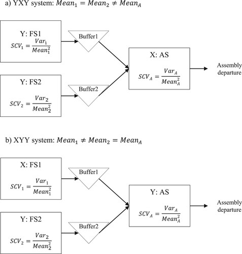
To capture the effect of variability transfer (VT) along with the effect of work transfer (WT) in the assembly system’s performance, a full factorial experimental design was used. Two types of assembly systems were considered in this study: (1) systems with equal mean processing times for the feeding stations, i.e. symmetrical feeding stations, and (2) systems with equal mean processing times between FS2 and AS, i.e. asymmetrical feeding stations. Using Baker and Powell’s (1995) nomenclature, where X represents the station that is different and Y represents the symmetrical stations in terms of mean processing times, systems with symmetrical feeding stations are YXY systems, whereas systems with asymmetrical feeding stations are XYY systems.

3.2.1. Experimental factors

Each experiment consisted of 5 different factors. The first factor modelled either YXY or XYY systems. The second factor modelled the mean processing times of the X station and, consequently, the mean processing times of the Y stations, as the sum of the processing times of all stations had to be equal to 3 to conserve the overall work content of the system, using the same procedure as previous studies (Baker, Powell, and Pyke 1993; Baker and Powell 1995; Sabuncuoglu, Erel, and Kok 2002). This factor analysed the impact of WT in assembly systems. Thus, (1) $\text{Mea}{\text{n}}_1+\text{Mea}{\text{n}}_2+\text{Mea}{\text{n}}_{\text{A}}=3$(1) where Mean_i, for i = 1, 2 and A, is the mean of the processing times of the corresponding station i, with 1 and 2 representing the feeding stations FS1 and FS2, respectively, and A representing the assembly station (AS).

The third and fourth factors modelled the values of the sum of variances (SumVar) in all stations of the system and the values of the sum of squared coefficients of variation (SumSCV) in all stations, respectively, to study the impact that different levels of overall variability have on the system. That is: (2) $\begin{array}{rl}\text{SumVar}& =\text{Va}{\text{r}}_1+\text{Va}{\text{r}}_2+\text{Va}{\text{r}}_{\text{A}}\end{array}$(2) (3) $\begin{array}{rl}\text{SumSCV}& =\text{SC}{\text{V}}_1+\text{SC}{\text{V}}_2+\text{SC}{\text{V}}_{\text{A}}\end{array}$(3) where Var_i, for i = 1, 2 and A, is the variance of the processing times of corresponding station i and SCV_i, for i = 1, 2 and A, is the squared coefficient of variation of the processing times of corresponding station i.

The last factor pertains to the unbalancing of variability in the system, or VT, by varying the values of Var or SCV for each station. This factor was the most important factor in the study, as it helped to investigate the effect of VT in assembly systems and discover whether supply or assembly variability had a greater impact on performance. Thus, the values of Var₁, Var₂ and Var_A and SCV₁, SCV₂ and SCV_A were modified by considering different combinations of variabilities to capture different behaviours, while keeping SumVar or SumSCV constant to directly assess VT. For instance, some experiments considered no Var in one feeding station and equal Var in the remaining stations, while others considered balanced variability in all stations, and yet others considered no Var in the assembly station and equal variabilities in the feeding stations. It is worth noting that no experiment considered a system where no variability was present in both feeding stations, as this system can effectively be modelled as a single-server queue with deterministic arrivals. Moreover, the experimental design assumes that systems with opposite Var values between feeding stations are equivalent, so ‘mirror’ systems have not been considered in the experimental design, e.g. a system with Var₁ = 0, Var₂ = 2 and Var_A = 1 is equivalent to a system with Var₁ = 2, Var₂ = 0 and Var_A = 1.

A summary of the factors and their values is shown in Table 2. Considering all the factorial combinations, a total of 1,368 experiments were run.

Table 2. Factors and their levels.

Factor	Levels	Values
Type of assembly system	2	YXY (X being AS) and XYY (X being FS1)
WT (work transfer)	19	MeanA (YXY) or Mean1 (XYY) from 0.1 to 1.9 minutes in 0.1 increments
Variability factor changed	2	Var or SCV
SumVar or SumSCV	3	1, 3 and 8
VT (variability transfer)	6	Var1 = 0 and Var2 = VarA = (1/2)SumVar  Var1 = 0, Var2 = (2/3)SumVar, VarA = (1/3)SumVar Var1 = (1/6)SumVar and Var2 = VarA = (5/12)SumVar Var1 = Var2 = VarA = (1/3) SumVar Var1 = Var2 = (5/12)SumVar and VarA = (1/6)SumVar Var1 = Var2 = (1/2)SumVar and VarA = 0 Equivalently for SCVi values

Therefore, contrary to what previous papers have done, this study considers WT and VT from the X station to Y stations, and vice-versa, in order to thoroughly investigate the effects of VT in various conditions and system loads.

Figure 1 shows an illustration of the two assembly system configurations considered in this study, X being the station that has a different mean processing time and Y being the two symmetrical stations in terms of mean processing time. Figure 1 also includes information about the associated parameters for each station (Mean_i, Var_i, SCV_i).

Figure 1. Illustration of the two types of assembly systems considered in the study.

Flow diagrams showing the characteristics of (a) symmetrical assembly systems and (b) asymmetrical assembly systems.

3.2.2. Experimental responses

To measure the impact of the experimental factors on performance, various responses were collected. Each experimental setting, or run, consisted of an estimated warm-up period of 1,000 minutes, following Welch’s procedure (Welch 1983), and a total run time of 10,000 minutes. A total of 100 independent replications were carried out per experiment using Simio Version 9.147 (Kelton, Smith, and Sturrock 2014).

Similar to previous studies, TH, as well as IDV, were measured. IDV measurements were complemented with the squared coefficient of variation of inter-departure times (IDSCV), as SCV is the most common way of measuring the variability of a production system’s output process. We also investigated the time (TA) that the ‘order’ would remain in the assembly station (buffer time + assembly operation) by considering the sum of the time that the first component part arriving at the AS must wait for a matching component plus the processing time of the two matching components in the actual assembly operation. However, because of the fact that this last measure greatly depends on the values of Mean_A, thus limiting the comparability of the results through the experimental values of Mean_A, a normalised version of this measure (nTA) was used.

Next, the formulas for measuring each response per replication are presented.

− the production rate for the jth replication of experiment k for all j = {1, 2, … , 100} and k = {1, 2, … , 1368} (4) $T{H}_{kj}=Productio{n}_j/10000$(4) where Production_j is the quantity of parts produced in the jth replication from the 1,000th minute to the 11,000th minute, for a total of 10,000 registered minutes.

− the inter-departure time between the ith departure and the (i-1)th departure of the jth replication of experiment k (X_kji) for all i = {2, 3, … , 10000}, j = {1, 2, … , 100} and k = {1, 2, … , 1368} (5) $X_{kji}=d_{kji}-d_{kj\left(i-1\right)}$(5) where d_kji is the departure time for the ith departure of the jth replication of experiment k

− the mean inter-departure time for the jth replication of experiment k (ID_kj) for all j = {1, 2, … , 100} and k = {1, 2, … , 1368} (6) $I{D}_{kj}=\frac{1}{Productio{n}_j}\sum _{i=1}^{Productio{n}_j}{X}_{kji}$(6)

− the variance of inter-departure times for the jth replication of experiment k (IDV_kj) for all j = {1, 2, … , 100} and k = {1, 2, … , 1368} (7) $ID{V}_{kj}=\frac{1}{Productio{n}_j-1}\sum _{i=1}^{Productio{n}_j}(X_{kji}-I{D}_{kj}{)}^2$(7)

− the squared coefficient of variation of inter-departure times for the jth replication of experiment k (IDSCV_kj) for all j = {1, 2, … , 100} and k = {1, 2, … , 1368} (8) $IDSC{V}_{kj}=ID{V}_{kj}/I{D_{kj}}^2$(8)

− the time spent in the AS for the ith departure for the jth replication of experiment k (t_kji) for all i = {1, 2, … , 10000}, j = {1, 2, … , 100} and k = {1, 2, … , 1368} (10) $t_{kji}=d_{kji}-\text{min}\left(a_{kji1},a_{kji2}\right)$(10) where a_jki1 is component 1’s arrival time at Buffer 1 and a_jki2 is component 2’s arrival time at Buffer 2

− the mean time spent in the AS for the jth replication of experiment k (TA_kj) for all j = {1, 2, … , 100} and k = {1, 2, … , 1368} (11) $T{A}_{kj}=\frac{1}{Productio{n}_j}\sum _{i=1}^{Productio{n}_j}{t}_{kji}$(11)

Therefore, the final responses that were considered in this study and are shown in Section 4 are the average of the responses of all replications per experiment. For example, the average throughput rate for experiment k (for all k = {1, 2, … , 1368}) was calculated as: (12) $T{H}_k=\frac{1}{100}\sum _{i=1}^{100}T{H}_{ki}$(12)

Taking this into consideration, the normalised mean time spent in the AS, depending on Mean_A and SumVar values (nTA_k) was calculated in the following manner: (13) $\begin{array}{r}nT{A}_k=\frac{T{A}_k}{\frac{1}{6}{\sum }_{l\in (Mean{A}_l=Mean{A}_k\wedge SumVa{r}_l=SumVa{r}_k}T{A}_l}\end{array}$(13)

It is worth noting that the equivalences Mean_Al =Mean_Ak and SumVar_l = SumVar_k in formula (13) reflect the fact that each value of TA_k will be divided by the average value of all the experiments with the same values for Mean_A and SumVar for the kth experiment.

3.3. Statistical analyses

Since the experimental results depend on random numbers, statistical analyses are needed to assess the statistical significance of the differences in the experiments with similar characteristics. Therefore, an ANOVA test (Walpole et al. 2011) was initially run to assess whether WT, on the one hand, and VT, on the other hand, resulted in statistically significant effects for all responses.

After the initial ANOVA test was conducted, a Duncan test (Duncan 1955) was carried out to analyse whether statistically significant differences existed for each response in multiple pairwise comparisons of experiments when WT or VT was performed. Finally, an additional ANOVA test was conducted for each response to analyse the impact of each factor.

As an aid to navigate the manuscript, Table 3 provides the reader with a list of the abbreviations used in the manuscript.

Table 3. List of abbreviations used throughout the manuscript.

Abbreviation	Variable
TH	Throughput rate of the assembly system
WT	Work transfer
IDV	Variance of inter-departure times
CV	Coefficient of variation
VT	Variability transfer
IDCV	Coefficient of variation of inter-departure times
Var	Variance
AS	Assembly station
FS1	Feeding station 1
FS2	Feeding station 2
SCV	Squared coefficient of variation
SumVar	Sum of variances of the three stations in the system
SumSCV	Sum of squared coefficients of variation of the three stations in the system
IDSCV	Squared coefficient of variation of inter-departure times
TA	Time spent in the assembly station
nTA	Normalised time spent in the assembly station
nρ	Normalised percentage capacity utilisation of the assembly station

4. Results

Initial ANOVA tests analysing the impact of WT or VT for YXY and XYY experiments showed that WT and VT had significant impacts on all the responses (see supplementary material). Moreover, very few experiments were found with no statistically significant differences when comparing experiments with different WT values.

It is worth noting that this section does not include the results regarding IDV, as the variability of the output of a system is usually represented as IDSCV because IDSCV can better convey the actual magnitude of the variability of the output and can be directly used as a measure of the variability of the input process in downstream stations (Buzacott and Shanthikumar 1993; W. Hopp and Spearman 2000).

Moreover, the factor SumSCV was only used to assess the effect of VT on IDSCV, and not on TH and nTA, because SumVar did not remain constant for experiments with different WT and different total system variances. Therefore, the results of varying SumSCV values on TH and nTA are not shown in this paper. Similarly, experiments where SumVar values changed were not considered in the results regarding IDSCV, as experiments with varying WT and Var resulted in systems with differing SumSCV.

4.1. YXY systems

4.1.1. Throughput rate, YXY systems

Results for YXY systems (symmetric feeding stations in terms of WT) show similar TH behaviour for all the values of SumVar analysed and confirm the results of previous studies where it was found that WT from the AS to the feeding stations (Mean_A < 1) resulted in better TH for experiments with the same VT.

In addition, Figure 2 illustrates the impact of VT on TH by showing how the highest TH was found in experiments with the lowest total feeding variability (red, solid line with rhomboid markers), while the lowest TH was found in experiments with higher total feeding variability (purple and yellow dashed lines with rectangular and circular markers, respectively). Interestingly, Figure 2 also shows that WT to feeding stations had a lower impact on TH with increasing overall variability of feeding stations. This is because experiments with high variability in feeding stations, e.g. Var₁ = Var₂ = 4 (yellow line in Figure 2 (b)), needed a significant amount of WT towards the feeding stations (Mean_A = 0.7, Mean₁ = Mean₂ = 1.15) to reach the highest experimental TH, contrary to experiments with lower feeding variability, e.g. Var₁ = 0, Var₂ = 0.5 (red line in Figure 2 (a)), which had the highest experimental TH (although not optimal, see Sabuncuoglu, Erel, and Kok 2002) in a balanced system.

Figure 2. TH for different levels of WT and VT, (a) SumVar = 1, (b) SumVar = 8, YXY systems.

Plots comparing the throughput rate of experiments with varying values of work and variability transfer for symmetrical scenarios with (a) SumVar = 1 and (b) SumVar = 8.

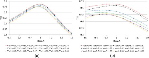
For symmetrical configurations, the effect of feeding station variability on TH seemed to be more dependent on the lowest Var value between both feeding stations than on the total Var for the feeding stations. The lowest Var value, by experimental design, always corresponded to FS1; thus, TH depended more on Var₁ than on Var₂, as shown in the ANOVAs (see supplementary material). For instance, experiments where Var₁ = 0, Var₂ = 5.33, Var_A = 2.67 and the total Var for the feeding stations was equal to 5.33 had higher TH than experiments where Var₁ = 1.33, Var₂ = Var_A = 3.33, where the total feeding Var was 4.67. If the minimum feeding variance was equal for two experiments, the experiment with the least total feeding variance would be the one with the highest TH, as shown in the contrasting experiments Var₁ = 0, Var₂ = Var_A = 4 vs. Var₁ = 0, Var₂ = 5.33, Var_A = 2.67. However, it should be noted that some of the experiments with similar feeding variability did not have statistically significant differences when considering the same WT (see supplementary material).

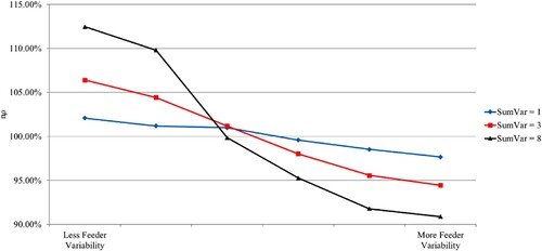
The dependency of TH on feeding variability can be explained by the effect that feeding variability, modelled primarily by Var₁ and then by the sum of Var₁ and Var₂, has on the utilisation of the AS, as higher utilisation of the stations has been linked to higher TH (Romero-Silva et al. 2019). To study this dependency, the normalised utilisation percentage of the AS, instead of the simple utilisation percentage, is used here as a measure of workload because comparisons among the values of real utilisation in experiments with different WT would produce very contrasting results. For instance, experiments with Mean_A = 1.9 have AS utilisation percentages around 80%, while experiments with Mean_A= 0.1 have AS utilisation percentages around 5%. Thus, by considering the percentage deviations from the mean (the normalised values), an average of all the experiments having the same Mean_A values can be calculated in order to assess the impact of feeding variability.

In this regard, Figure 3 suggests that higher feeding variability results in lower normalised utilisation (nρ) of the AS for all the experimental values of SumVar. This behaviour could be explained by the higher synchronisation time (De Boeck and Vandaele 2011) of the components caused by higher feeding variability, which would cause the AS to idle while waiting for the matching part; this would result in reduced utilisation and a lower rate of production (TH). In addition, Figure 3 shows that the higher the total variability of the system is (SumVar), the bigger the impact that feeding variability has on nρ, explaining why higher feeding variability affects TH in symmetric assembly systems.

Figure 3. Normalised percentage capacity utilisation levels of the assembly station by different feeding variability and SumVar values, YXY systems.

Plot showing the effect of feeding variability on the normalised percentage capacity utilisation levels of the assembly station for different SumVar values in symmetrical systems.

4.1.2. Squared coefficient of variation of inter-departure times, YXY systems

The behaviour of IDSCV for YXY systems, shown in Figure 4, is similar to the behaviour of IDSCV in single-server queues since it mostly depends on the SCV of inter-arrival times (SCV₁ and SCV₂) for low values of server utilisation; yet for high values of server utilisation, e.g. Mean_A = 1.9, it mostly depends on SCV_A. This behaviour is consistent with single-server systems, since the IDSCV behaves like a quadratic function (Buzacott and Shanthikumar 1993), showing a ‘hill’ for intermediate levels of WT to feeding stations, particularly in experiments where SumSCV = 1 (see Figure 4 (a)).

Figure 4. IDSCV for different values of WT and VT, (a) SumSCV = 1, (b) SumSCV = 8, YXY systems.

Plots comparing the squared coefficient of variation of inter-departure times for experiments with varying values of work and variability transfer for symmetrical scenarios with (a) SumVar=1 and (b) SumVar=8.

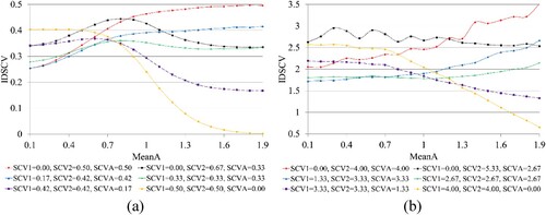
For experiments with SumSCV = 8 and symmetric feeding stations (see Figure 4 (b)), the behaviour of IDSCV does not behave as a quadratic function, as has been previously suggested (Buzacott and Shanthikumar 1993; W. Hopp and Spearman 2000), and resembles more to a polynomial function, particularly for experiments where SCV₁ = 0.00 (red and black lines in Figure 4 (b)). However, it is worth noting that IDSCV values for some of these experiments did not have statistically significant differences (see supplementary material) when comparing experiments with equal SCV values but different Mean_A values.

4.1.3. Time spent in the assembly station, YXY systems

Delivery times are critical for some manufacturing markets, as customers require a rapid response, starting with the placement of the order. Therefore, it is relevant to also investigate the effect that variability has on the time that orders spend in the assembly system. In order to produce easily interpretable results and conclusions regarding the effect of VT on time spent in the assembly station, a direct measure of the amount of time that a complete order stays in the system was calculated, namely, the time an arriving part spends waiting for the complementary part to arrive plus the time both parts spend being processed in the AS.

As explained in subsection 3.2.2, the time spent in the assembly station was measured by a normalised measurement (nTA) in order to make it possible to compare the effect of different values of VT throughout all the values of Mean_A, as higher values of Mean_A will clearly result in higher TA values.

Figure 5 shows how the effect of variability on nTA changes with increasing values of SumVar, as experiments with no variance or low variance in one of the feeding stations produce bad relative performance when SumVar = 1 but good relative performance when SumVar = 8. In contrast, experiments with low variance or no variance in the AS produce a good relative performance when SumVar = 1 and Mean_A < 1 but bad performance with regard to nTA when SumVar = 8 and Mean_A > 1.

Figure 5. nTA for different values of WT and VT, (a) SumVar = 1, (b) SumVar = 8, YXY systems.

Plots comparing the normalised time spent in the assembly station for experiments with varying values of work and variability transfer for symmetrical scenarios with (a) SumVar=1 and (b) SumVar=8.

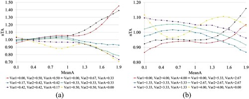
These results suggest that transferring variability to the AS will not produce good results with regard to nTA when the total system variability is low, but doing so will produce good results when total variability is high; the exception is when the workload of the AS is high, because the combination of both variability and workload will clearly produce bad results. On the other hand, transferring all the variability from the AS to the feeding stations would seem to be good practice with regard to nTA in low variability scenarios, except when the feeding stations are very loaded (low values of Mean_A).

It is worth noting that the results shown in Figure 5 cannot be directly compared across different values of Mean_A, as the normalised values are the result of a division between the actual TA value and the mean TA of all the experiments with the same Mean_A. Thus, Figure 5 can only be studied ‘vertically’, i.e. directly comparing VT differences and not WT differences, despite the fact that figure lines are comprised of experiments with different values of WT for consistency throughout the paper.

4.2. XYY systems

To have a more complete picture of the effect of VT on assembly systems, we also studied assembly systems where FS2 has the same work content as the AS, leaving FS1 as the X component of the system.

4.2.1. Throughput rate, XYY systems

The effect of variability on TH regarding XYY systems is similar to its effect on YXY systems, as lower levels of feeding variability will result in higher TH (Figure 6). However, when SumVar ≤ 3 and one feeding station is actually a severe system bottleneck (Mean₁ > 1.6), the best performing system in terms of TH is, interestingly, the variability-balanced system where Var values for all stations are equal; the worst performing system in that setting, in contrast, is the one where the highest variance is found in one of the feeding stations, e.g. Var₁ = 0.33, Var₂ = 0.67 and Var_A = 0 (Figure 6 (a)). Thus, when one feeding station is a severe bottleneck, the values of min(Var₁, Var₂) and max(Var₁, Var₂) seem to be more relevant for the resulting highest and lowest values of TH in low or moderately variable assembly systems, despite the fact that the differences between the values of TH tend to be minimal but statistically significant (see supplementary material) in these scenarios.

Figure 6. TH for different levels of WT and VT, (a) SumVar = 1, (b) SumVar = 8, XYY systems.

Plots comparing the throughput rate of experiments with varying values of work and variability transfer for asymmetrical scenarios with (a) SumVar=1 and (b) SumVar=8.

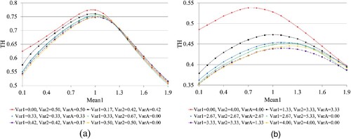
Additionally, XYY scenarios where SumVar ≥ 3 and Var₁ = 0 (red, solid line with rhomboid markers in Figure 6 (b)) were the only experiments in our study where WT out of a feeding station (towards the AS and the other feeding station by experimental design) resulted in the best experimental TH, which contrast with previous results in the literature. This might be explained by the fact that the assembly system is taking advantage of having no variability in FS1 by reducing its workload, which in turn would procure a better rate of arrival of components to the assembly station and increase the TH, even if the other feeding station has an increased workload.

It is worth noting that Figure 6 shows TH depending on Mean₁ and not on Mean_A, to relate TH with the non-symmetrical X station. Moreover, the ANOVA test regarding TH for XYY systems (see supplementary material) resulted in results that were very similar to those for YXY systems, where Var₁, Var₂ and Mean_A all had highly significant impacts.

4.2.2. Squared coefficient of variation of inter-departure times, XYY systems

Experimental results for IDSCV regarding XYY systems (Figure 7) show an even higher effect of SCV₁ on IDSCV when the values of Mean_A are very low, as in this case FS1 is very loaded and becomes the severe bottleneck; whereas at higher values of Mean_A IDSCV is more dependent on SCV₂ values for XYY systems than for YXY systems. This is because Mean₂ values are equal to Mean_A values in XYY settings, creating a higher dependency on SCV₂ for higher values of both Mean_A and Mean₂.

Figure 7. IDSCV for different values of WT and VT, (a) SumSCV = 1, (b) SumSCV = 8, XYY systems.

Plots comparing the squared coefficient of variation of inter-departure times for experiments with varying values of work and variability transfer for asymmetrical scenarios with (a) SumVar=1 and (b) SumVar=8.

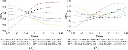
In addition, Figure 7 (b) shows a ‘valley’ in the shape of the line of the IDSCV results for some VT values when SumSCV = 8, a characteristic that is the opposite of the behaviour of IDSCV for YXY systems when SumSCV = 1 (Figure 4 (a)). Figure 7 (b) also shows how the results for experiments where SumSCV = 8 were highly fluctuating, as the lines in the figure are not ‘smooth’ and some experiments with the same VT did not have statistically significant differences (see supplementary material) among them.

The behaviour of XYY systems with balanced VT (SCV₁ = SCV₂ = SCV_A) is very peculiar, as experiments show that IDSCV is reduced in balanced or somewhat balanced systems regarding WT. When SCV is equal in all the stations in XYY systems, a difference in the capacity of any station will produce an increase in the variability of inter-departure times, contrary to YXY systems with balanced VT, where IDSCV is reduced when the utilisation of the assembly system is minimal.

4.2.3. Time spent in the assembly station, XYY systems

Figure 8 (a) shows how the effect of VT on nTA for XYY systems is similar to the effect caused by VT on YXY systems (Figure 5 (a)) since higher values of Var_A will produce higher relative cycle times when SumVar = 1, whereas lower values of Var_A will reduce nTA in the entire range of AS values of utilisation.

Figure 8. nTA for different values of WT and VT, (a) SumVar = 1, (b) SumVar = 8, XYY systems.

Plots comparing the normalised time spent in the assembly station for experiments with varying values of work and variability transfer for asymmetrical scenarios with (a) SumVar=1 and (b) SumVar=8.

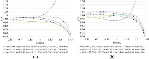
However, the effect of variability on nTA regarding XYY systems when SumVar = 8 seems to be highly dependent on the load that each station has in relation to its variability. For instance, when Mean_A is lightly loaded (Mean₁ is highly loaded), either a low Var_A or a low Var₁, respectively, will produce lower nTA. In contrast, when considering a more heavily loaded Mean_A, more balanced VT experiments resulted in better nTA. Unbalanced VT experiments had, by experimental design, a high Var₂ which, in interaction with a highly loaded Mean₂ (Mean_A = Mean₂ in XYY experiments), resulted in higher nTA values.

The impact of these interactions between variability and station load can be clearly seen in the results from the ANOVA test for nTA (see supplementary material) by looking at how nTA was affected by the interactions between Mean_A² and the different values of Var. Furthermore, the ANOVA test for nTA also shows that Var₁ and Var₂ have a higher effect on nTA for XYY experiments than Var_A does, a result that differs from the YXY experiments, where Var_A had the largest impact of all the single factors.

Thus, in low variability contexts, it would seem that Var_A is the most critical factor in reducing TA in XYY systems, since the impact of the time that the first arriving component has to wait for the second component, a consequence of feeding variability, appears to be less critical. On the contrary, in high variability contexts, TA could be affected by the variability of either the feeding or assembly stations since the time spent waiting for the remaining component and the actual processing time in the AS are both critical for the resulting TA.

5. Discussion

In order to answer research questions (1) and (2), this section has been divided into two subsections that analyse the experimental results in terms of the similarities (subsection 5.1) and differences (Subsection 5.2) between the two simple assembly systems studied here. Subsections 5.1 and 5.2 also discuss how the results from this study compare with previous research and highlight the new insights from the current study. We end this section by describing the managerial insights of the study (subsection 5.3).

5.1. Variability effects shared by YXY and XYY systems

A result that appeared in most experiments was that TH was highly dependent on the variability of feeding stations because, in order to increase TH, the variance of at least one feeding station needed to be transferred to the AS. For instance, the highest TH was reached when Var₁ = 0. Furthermore, in line with the conclusions of Bhatnagar and Chandra (1994), we found that the amount of WT to the feeding stations that was needed to increase TH was even more critical, i.e. more WT was needed when the variability of the feeding stations was higher, with rising feeding variability, thus creating the need to increase the capacity of the AS even more in order to compensate for the increased waiting time during component matching due to feeding variability.

Despite the fact that the impact of VT on IDSCV is more difficult to assess because it strongly depends on the utilisation of the AS, our results show an interesting effect of feeding variability on IDSCV in capacity-balanced systems with low variability: specifically, IDSCV in WT-balanced systems can be reduced by transferring variability from the AS to the feeding stations, a conclusion that supports the conclusions drawn by Sabuncuoglu, Erel, and Kok (2002) regarding the effects of VT on IDSCV. This behaviour in balanced systems could be caused by the fact that IDSCV is more dependent on SCV_A than on SCV₁ and SCV₂, even in WT-balanced systems, as the bottleneck of the operation in WT-balanced systems is the processing time of the AS, a characteristic that is shown by the need to transfer work out of the AS.

On the other hand, the impact of feeding variability on nTA changed considerably as values of SumVar changed. In somewhat capacity-balanced systems, nTA tended to be reduced with increasing values of Var₁ in systems where SumVar = 1, but nTA increased as values of Var₁ increased when considering systems where SumVar = 8. Thus, these results contrast with Chen et al.’s (2022) as we found that the time spent in the assembly station is quite sensitive to changes in both total system variance and feeding station variance.

Our results also suggest that increasing values of feeding variability in low variability scenarios result in a reduction in TH. But it also results in a reduction of IDSCV, which could help the performance of a downstream station by reducing the inter-arrival SCV (Whitt 1980).

Thus, although the effect of variability on the performance of assembly systems is a topic where many different conclusions can be provided, question (1) of the study can be answered in the following manner: The variability of feeding stations has a stronger effect on the performance of assembly systems, particularly on TH, than the effect caused by the variability of the assembly station. These results support the conclusions given by De Boeck and Vandaele (2008; 2011) but not the conclusions provided by Sabuncuoglu, Erel, and Kok (2002), as we found that variability transfer towards the AS produced better results than VT to the feeding stations, in contrast to the effect of WT.

5.2. Differences in variability effects on YXY and XYY systems

An interesting and contrasting result regarding TH from previous work (Baker, Powell, and Pyke 1993; Sabuncuoglu, Erel, and Kok 2002) is shown in Figure 6 (b) where, for XYY experiments with Var₁ = 0, Var₂ = 4 and Var_A = 4, TH is not maximised with WT to the feeding stations but TH is increased when WT is moved from FS1 to the other stations. This particular behaviour is caused by allowing FS1 to work more quickly with no variability, a combination that seems to produce a better overall component supply rhythm, despite the fact that FS2 would have more workload in this scenario.

Thus, a straightforward answer to question (2) of the study would be difficult to provide because of the many similarities as well as particular differences found between YXY and XYY systems. However, a very interesting result regarding XYY systems that clearly departs from previous results (Sabuncuoglu, Erel, and Kok 2002; Krishnamurthy, Suri, and Vernon 2004) considering symmetrical systems is the fact that VT had a higher impact on TH values than WT for scenarios with high total variance, as illustrated in Figure 6 (b) by the bigger differences in TH values found in experiments with different Var₁ values (comparing values corresponding to different lines but equal values in the horizontal axis in Figure 6 (b)) when compared with the smaller differences found in experiments with different Mean₁ values (comparing values corresponding to the same line in Figure 6 (b)). This result was not true for YXY systems as our results for these systems are in line with previous results showing that WT has a bigger impact on TH than VT.

Furthermore, it could be concluded that YXY systems seem to share some characteristics with single-server systems given that the overall results for IDSCV and nTa in YXY systems are similar regarding the effect of variability and server utilisation (see Romero-Silva et al. 2019 for a summary of these effects). However, XYY systems do not seem to behave like single-server systems and they cannot be modelled with the same approximations, particularly when the X station is a hard bottleneck, since the utilisation factor in all single-server formulas becomes unfit for XYY systems.

5.3. Managerial insights

Results from the study consistently suggest that reducing the variability of supply (feeding) stations increases the output of an assembly system, even if the variability of one feeding station (and the assembly station) is increased while the other is reduced. This is due to the fact that reducing the variability of feeding processes increases the capacity utilisation of the assembly station by reducing the time it takes to match the two components needed to start the assembly operation. Thus, working to reduce the variability of even one component supplier will help manufacturing firms with converging components to increase their throughput. Seen from another perspective, any efforts to reduce the variability of the assembly station process cannot overcome the negative impact on throughput that high supply (feeding) variability produces.

Even though the highest experimental throughput for low variability systems (SumVar = 1) was equal in YXY and XYY configurations and was found in WT-balanced systems, assembly systems with higher total variability (SumVar ≥ 3) should arrange their supply stations in an asymmetrical manner (XYY configuration) by transferring variability and work simultaneously out of one of the supply (feeding) stations, as the highest experimental throughput for highly variable systems was found in systems with asymmetrical supply (feeding) stations with less work content than the assembly station (0.7 ≤ Mean₁ ≤ 0.9) and no variance (Var₁ = 0).

This means that industries with high process control where supply (feeding components) variability is minimal, such as the automotive sector, are better served in terms of production rate by investing more efforts in (slightly) increasing the production rate of the assembly station as compared with the production rate of the feeding stations. These low-variability industries should also prioritise reducing supply (feeding components) variability instead of assembly station variability. For industries where the feeding processes variability is not under control due to inherently variable upstream processes or black/grey swan events (Akkermans and Wassenhove 2013) such as the Covid-19 pandemic, improvement efforts to increase the production rate should focus on reducing the variability of at least one feeding process while also increasing the production rate of the feeding process with reduced variability.

However, when the main objective of a manufacturing firm is to have a short delivery time (also known as flow time or cycle time), reducing supply variability from the feeding stations is only suggested for high variance environments as low variance experimental environments were better served in terms of cycle time by reducing the variability of the assembly operation because the variance of supply is not as high to have an influence on the resulting total cycle time.

6. Conclusions, limitations and future research

This study was concerned with investigating the effect that supply variability (or the variability of feeding stations) has on the performance of assembly systems in comparison with the effect of the variability of the actual assembly operation. In contrast to previous studies on the topic, we investigated the effect of the variability of feeding stations on the performance of asymmetrical assembly systems by comparing experiments with identical total variance and work content but different variance and work content allocations to the system’s stations.

Simulation experiments show that throughput is significantly affected by increasing the variability of feeding processes while decreasing the variability in the assembly station. Thus, it can be concluded that variability in supply (feeding) operations is more critical than variability in assembly operations regarding throughput performance in our experimental setting. Furthermore, results from this study confirmed previous studies’ conclusion that transferring work from the assembly station to the feeding stations increased the system’s throughput, with the exception of systems where one of the feeding stations was the capacity bottleneck and did not have variability. In this particular case, the best policy was to transfer work from this feeding station to the assembly station.

Results from this study also suggest that the variability of the output process of a simple assembly system, measured by the squared coefficient of variation of inter-departure times, is highly dependent on the utilisation values of the bottleneck station of the system, similar to the behaviour of single-server queues. Furthermore, the manner in which the average time spent in the assembly station was reduced depended on the values of the sum of variances for each scenario. In scenarios with low total variability, the average time spent in the assembly station was reduced by transferring variability to the feeding stations (reducing the variability in the assembly station) whereas in scenarios with high total variability the average time spent in the assembly station was reduced by transferring variability to the assembly station (reducing variability in the feeding stations).

The main limitation of this study is that the results are not analytically tractable because of the complexity of the system and the experimental design; therefore, these results could not be validated by mathematical procedures, as recent studies have done (see, e.g. N. Chen et al. 2022; Shen and Li 2021). Despite this limitation, our methodological approach allowed us to systematically analyse the effect of the variability of feeding stations on the performance of assembly systems by being able to incorporate many degrees of freedom in terms of variability modelling and carrying out an extensive set of experiments, in line with previous simulation-based studies investigating complex assembly systems (see, e.g. Romero-Silva and Shaaban 2019; Ostermeier 2022; Thürer et al. 2020). Furthermore, as shown in Duncan’s tests (see supplementary material), some experiments did not have statistically significant differences when compared with similarly valued experiments. However, as the bulk of the results provided consistent and plausible conclusions and did have statistically significant differences, we believe that they provide useful and interesting conclusions to better understand the different levels of impact that variability of feeding processes and assembly station variability have on the performance of assembly systems.

In addition, the results for XYY systems could be limited by the experimental design because FS1 was selected as the X station and Var₁ was always equal to or lower than Var₂ in order to have some consistency with YXY experiments. Thus, further experiments will be needed to investigate the behaviour of XYY systems when the X station has higher Var or SCV than all the other stations. Furthermore, as the values of SumVar and SumSCV remained constant when VT varied, there was interdependency among the variability values of all stations, i.e. when the variability of feeding processes increased the assembly variability decreased, and vice-versa. This experimental design produced results with no influence of added variance to the system but prevented the study from investigating the single effect that variability of feeding processes has on the performance of assembly systems when assembly variability is held constant. Thus, more research is needed to discover the singular effects that feeding or assembly variabilities have on performance.

Finally, future work could focus on studying the impact of the variability of multiple feeding processes or even more complex assembly lines with multiple merging processes on assembly line performance since one of the limitations of this study is that we considered a simple assembly system with only two feeding stations. In reality, assembly lines for certain industrial sectors are much more complex as they have multiple components merging into the final assembly line and much more complex production flows, so the current study provides very initial insights into this problem. Moreover, future research could study how variability affects different tactical feeding policies, such as, line stocking, boxed supply, and stationary kitting (Schmid and Limère 2019), since these mechanisms could be influenced differently by the variability of upstream processes.

Supplementary material

• - Duncan’s tests

• - ANOVA tests

Data availability statement

The data that support the findings of this study are available from the corresponding author, RRS, upon reasonable request.

Disclosure statement

No potential conflict of interest was reported by the author(s).

Additional information

Notes on contributors

Rodrigo Romero-Silva

Rodrigo Romero-Silva is an Assistant Professor at the Operations Research and Logistics Group of Wageningen University & Research (The Netherlands) and an Assistant Professor at the Faculty of Engineering at Universidad Panamericana (Mexico). He received his Ph.D. in Industrial Engineering from the University of Navarra (Spain) in 2012. Rodrigo’s research is focused on understanding the behaviour of stochastic and dynamic production and logistics systems while creating applicable planning approaches for their operation. Before joining academia, Rodrigo worked as a data analyst in the retail sector.

Margarita Hurtado-Hernández

Margarita Hurtado-Hernandez is an academician oriented towards the application of knowledge obtaining positive results in organisations, through business training and the higher education of young professionals. She is the Director of graduate programmes at the Faculty of Engineering of Universidad Panamericana (Mexico) and a teacher – researcher at the Operations Management Department. She has a Ph.D. in Operations Research and Management Science and has been the leader on a number of research projects on how to improve the performance of organisations through the systems thinking approach. She has published three books on how to address real problems using systems thinking.

References

- Akkermans, Henk A, and Luk N Van Wassenhove. 2013. “Searching for the Grey Swans: The Next 50 Years of Production Research.” International Journal of Production Research 51 (23–24): 6746–6755. doi:10.1080/00207543.2013.849827.
- Baker, Kenneth R, and Dominik Altheimer. 2012. “Heuristic Solution Methods for the Stochastic Flow Shop Problem.” European Journal of Operational Research 216 (1): 172–177. doi:10.1016/j.ejor.2011.07.021.
- Baker, Kenneth R, and Stephen G Powell. 1995. “A Predictive Model for the Throughput of Simple Assembly Systems.” European Journal of Operational Research 81 (2): 336–345. doi:10.1016/0377-2217(93)E0283-4.
- Baker, Kenneth R, Stephen G Powell, and David F Pyke. 1993. “Optimal Allocation of Work in Assembly Systems.” Management Science 39 (1): 101–106. doi:10.1287/mnsc.39.1.101.
- Ben-Ammar, Oussama, and Alexandre Dolgui. 2018. “Optimal Order Release Dates for Two-Level Assembly Systems with Stochastic Lead Times at Each Level.” International Journal of Production Research 56 (12): 4226–4242. doi:10.1080/00207543.2018.1449268.
- Bhatnagar, Rohit, and Pankaj Chandra. 1994. “Variability in Assembly and Competing Systems: Effect on Performance and Recovery.” IIE Transactions 26 (5): 18–31. doi:10.1080/07408179408966625.
- Bock, Stefan, and Nils Boysen. 2021. “Integrated Real-Time Control of Mixed-Model Assembly Lines and Their Part Feeding Processes.” Computers & Operations Research 132: 105344. doi:10.1016/j.cor.2021.105344.
- Boeck, Liesje De, and Nico Vandaele. 2008. “Coordination and Synchronization of Material Flows in Supply Chains: An Analytical Approach.” International Journal of Production Economics 116 (2): 199–207. doi:10.1016/j.ijpe.2008.06.010.
- Boeck, Liesje De, and Nico Vandaele. 2011. “Analytical Analysis of a Generic Assembly System.” International Journal of Production Economics 131 (1): 107–114. doi:10.1016/j.ijpe.2010.04.036.
- Borodin, Valeria, Alexandre Dolgui, Faicel Hnaien, and Nacima Labadie. 2016. “Component Replenishment Planning for a Single-Level Assembly System Under Random Lead Times: A Chance Constrained Programming Approach.” International Journal of Production Economics 181: 79–86. doi:10.1016/j.ijpe.2016.02.017.
- Boudella, Mohamed El Amine, Evren Sahin, and Yves Dallery. 2018. “Kitting Optimisation in Just-in-Time Mixed-Model Assembly Lines: Assigning Parts to Pickers in a Hybrid Robot–Operator Kitting System.” International Journal of Production Research 56 (16): 5475–5494. doi:10.1080/00207543.2017.1418988.
- Boxma, Onno, Offer Kella, and Liron Ravner. 2019. “Fluid Queues with Synchronized Output.” Operations Research Letters 47 (6): 629–635. doi:10.1016/j.orl.2019.10.007.
- Buzacott, John, and J. G. Shanthikumar. 1993. Stochastic Models of Manufacturing Systems. 1st ed. Englewood Cliffs, New Jersey: Prentice-Hall.
- Calzavara, Martina, Serena Finco, Daria Battini, Fabio Sgarbossa, and Alessandro Persona. 2021. “A Joint Assembly Line Balancing and Feeding Problem (JALBFP) Considering Direct and Indirect Supply Strategies.” International Journal of Production Research 0 (0): 1–19. doi:10.1080/00207543.2021.1968527.
- Caputo, Antonio Casimiro, Pacifico Marcello Pelagagge, and Paolo Salini. 2018. “Selection of Assembly Lines Feeding Policies Based on Parts Features and Scenario Conditions.” International Journal of Production Research 56 (3): 1208–1232. doi:10.1080/00207543.2017.1407882.
- Caputo, Antonio Casimiro, Pacifico Marcello Pelagagge, and Paolo Salini. 2021. “A Model for Planning and Economic Comparison of Manual and Automated Kitting Systems.” International Journal of Production Research 59 (3): 885–908. doi:10.1080/00207543.2020.1711985.
- Chen, Nan, Ningjian Huang, Robert Radwin, and Jingshan Li. 2022. “Analysis of Assembly-Time Performance (ATP) in Manufacturing Operations with Collaborative Robots: A Systems Approach.” International Journal of Production Research 60 (1): 277–296. doi:10.1080/00207543.2021.2000060.
- Chen, Junhao, Xiaoliang Jia, and Qixuan He. 2021. “A Novel Bi-Level Multi-Objective Genetic Algorithm for Integrated Assembly Line Balancing and Part Feeding Problem.” International Journal of Production Research 0 (0): 1–24. doi:10.1080/00207543.2021.2011464.
- Choi, Thomas Y, Sriram Narayanan, David Novak, Jan Olhager, Jiuh-Biing Sheu, and Frank Wiengarten. 2021. “Managing Extended Supply Chains.” Journal of Business Logistics 42 (2): 200–206. doi:10.1111/jbl.12276.
- Dolgui, Alexandre, Fabio Sgarbossa, and Marco Simonetto. 2022. “Design and Management of Assembly Systems 4.0: Systematic Literature Review and Research Agenda.” International Journal of Production Research 60 (1): 184–210. doi:10.1080/00207543.2021.1990433.
- Duncan, David B. 1955. “Multiple Range and Multiple F Tests.” Biometrics 11 (1): 1–42. doi:10.2307/3001478.
- Ebrahimi, Mojtaba, Mehdi Mahmoodjanloo, Behnam Einabadi, Armand Baboli, and Eva Rother. 2022. “A Mixed-Model Assembly Line Sequencing Problem with Parallel Stations and Walking Workers: A Case Study in the Automotive Industry.” International Journal of Production Research 0 (0): 1–20. doi:10.1080/00207543.2021.2022801.
- Guo, Jun, Zhipeng Pu, Baigang Du, and Yibing Li. 2021. “Multi-Objective Optimisation of Stochastic Hybrid Production Line Balancing Including Assembly and Disassembly Tasks.” International Journal of Production Research 60 (0): 2884–2900. doi:10.1080/00207543.2021.1905902.
- Harrison, J Michael. 1973. “Assembly-like Queues.” Journal of Applied Probability 10 (2). 354–367. http://www.jstor.org/stable/3212352.
- He, Beixiang, Yunan Liu, and Ward Whitt. 2016. “STAFFING A SERVICE SYSTEM WITH NON-POISSON NON-STATIONARY ARRIVALS.” Probability in the Engineering and Informational Sciences 30 (4): 593–621. doi:10.1017/S026996481600019X.
- Hopp, Wallace J, and John T Simon. 1989. “Bounds and Heuristics for Assembly-Like Queues.” Queueing Systems 4 (2): 137–155. doi:10.1007/BF01158549.
- Hopp, Wallace J, and John T Simon. 1993. “Estimating Throughput in an Unbalanced Assembly-Like Flow System.” International Journal of Production Research 31 (4): 851–868. doi:10.1080/00207549308956762.
- Hopp, Wallace, and Mark Spearman. 2000. Factory Physics. Second. McGraw-Hill.
- Hu, S. J., J. Ko, L. Weyand, H. A. ElMaraghy, T. K. Lien, Y. Koren, H. Bley, G. Chryssolouris, N. Nasr, and M. Shpitalni. 2011. “Assembly System Design and Operations for Product Variety.” CIRP Annals 60 (2): 715–733. doi:10.1016/j.cirp.2011.05.004.
- Kelton, W David, Jeffrey S Smith, and David T Sturrock. 2014. Simio and Simulation: Modeling, Analysis, Applications. 1st ed. Sewickley, PA: Simio LLC.
- Krishnamurthy, Ananth, Rajan Suri, and Mary Vernon. 2004. “Analysis of a Fork/Join Synchronization Station with Inputs from Coxian Servers in a Closed Queuing Network.” Annals of Operations Research 125 (1): 69–94. doi:10.1023/B:ANOR.0000011186.14865.19.
- Louly, M. A., A. Dolgui, and F. Hnaien. 2008. “Optimal Supply Planning in MRP Environments for Assembly Systems with Random Component Procurement Times.” International Journal of Production Research 46 (19): 5441–5467. doi:10.1080/00207540802273827.
- Lucas, Thomas W., W. David Kelton, Paul J. Sánchez, Susan M. Sanchez, and Ben L. Anderson. 2015. “Changing the Paradigm: Simulation, Now a Method of First Resort.” Naval Research Logistics (NRL) 62 (4): 293–303. doi:10.1002/nav.21628.
- Manitz, Michael, and Horst Tempelmeier. 2012. “The Variance of Inter-Departure Times of the Output of an Assembly Line with Finite Buffers, Converging Flow of Material, and General Service Times.” OR Spectrum 34 (1): 273–291. doi:10.1007/s00291-010-0216-1.
- Ostermeier, Frederik Ferid. 2022. “On the Trade-Offs Between Scheduling Objectives for Unpaced Mixed-Model Assembly Lines.” International Journal of Production Research 60 (3): 866–893. doi:10.1080/00207543.2020.1845914.
- Polat, Olcay, Can B Kalayci, Özcan Mutlu, and Surendra M Gupta. 2016. “A Two-Phase Variable Neighbourhood Search Algorithm for Assembly Line Worker Assignment and Balancing Problem Type-II: An Industrial Case Study.” International Journal of Production Research 54 (3): 722–741. doi:10.1080/00207543.2015.1055344.
- Powell, Stephen G, and David F Pyke. 1998. “Buffering Unbalanced Assembly Systems.” IIE Transactions 30 (1): 55–65. doi:10.1080/07408179808966437.
- Romero-Silva, Rodrigo, Erika Marsillac, Sabry Shaaban, and Margarita Hurtado-Hernández. 2019. “Serial Production Line Performance Under Random Variation: Dealing with the ‘Law of Variability’. doi:10.1016/j.jmsy.2019.01.005.
- Romero-Silva, Rodrigo, and Sabry Shaaban. 2019. “Influence of Unbalanced Operation Time Means and Uneven Buffer Allocation on Unreliable Merging Assembly Line Efficiency.” International Journal of Production Research 57 (6): 1645–1666. doi:10.1080/00207543.2018.1495344.
- Romero-Silva, Rodrigo, Sabry Shaaban, Erika Marsillac, and Zouhair Laarraf. 2021. “The Impact of Unequal Processing Time Variability on Reliable and Unreliable Merging Line Performance.” International Journal of Production Economics 235 (May): 108108. doi:10.1016/j.ijpe.2021.108108.
- Sabuncuoglu, Ihsan, Erdal Erel, and A. Gurhan Kok. 2002. “Analysis of Assembly Systems for Interdeparture Time Variability and Throughput.” IIE Transactions 34 (1): 23–40. doi:10.1080/07408170208928847.
- Schmenner, Roger W, and Morgan L Swink. 1998. “On Theory in Operations Management.” Journal of Operations Management. doi:10.1016/S0272-6963(98)00028-X.
- Schmid, Nico André, and Veronique Limère. 2019. “A Classification of Tactical Assembly Line Feeding Problems.” International Journal of Production Research 57 (24): 7586–7609. doi:10.1080/00207543.2019.1581957.
- Schmid, Nico André, Veronique Limère, and Birger Raa. 2021. “Mixed Model Assembly Line Feeding with Discrete Location Assignments and Variable Station Space.” Omega 102: 102286. doi:10.1016/j.omega.2020.102286.
- Schoemig, Alexander K. 1999. “On the Corrupting Influence of Variability in Semiconductor Manufacturing.” Simulation Conference Proceedings, 1999 Winter 1: 837–842. doi:10.1145/324138.324532.
- Shen, Xiaoxiao, and Na Li. 2021. “Scheduling Policies Analysis for Matching Operations in Bernoulli Selective Assembly Lines.” International Journal of Production Research 0 (0): 1–24. doi:10.1080/00207543.2021.1939903.
- Som, Pradip, W. E. Wilhelm, and R. L. Disney. 1994. “Kitting Process in a Stochastic Assembly System.” Queueing Systems 17 (3): 471–490. doi:10.1007/BF01158705.
- Sönmez, Erkut, Alan Scheller-Wolf, and Nicola Secomandi. 2017. “An Analytical Throughput Approximation for Closed Fork/Join Networks.” INFORMS Journal on Computing 29 (2): 251–267. doi:10.1287/ijoc.2016.0727.
- Takahashi, Misa, Hideo Ōsawa, and Takehisa Fujisawa. 2000. “On a Synchronization Queue with Two Finite Buffers.” Queueing Systems 36 (1): 107–123. doi:10.1023/A:1019127002333.
- Thürer, Matthias, Haiwen Zhang, Mark Stevenson, Federica Costa, and Lin Ma. 2020. “Worker Assignment in Dual Resource Constrained Assembly Job Shops with Worker Heterogeneity: An Assessment by Simulation.” International Journal of Production Research 58 (20): 6336–6349. doi:10.1080/00207543.2019.1677963.
- Varma, Subir, and Armand M Makowski. 1994. “Interpolation Approximations for Symmetric Fork-Join Queues.” Performance Evaluation 20 (1): 245–265. doi:10.1016/0166-5316(94)90016-7.
- Walpole, Ronald E, Raymond H Myers, Sharon L Myers, and Keying Ye. 2011. Probability and Statistics for Engineers and Scientists. 9th ed. New York, NY: Pearson.
- Welch, P. D. 1983. “The Statistical Analysis of Simulation Results.” In The Computer Performance Modeling Handbook, edited by S. S. Lavenberg, 268–328. New York: Academic Press.
- Whitt, Ward. 1980. “The Effect of Variability in the GI/G/s Queue.” Journal of Applied Probability 17 (4): 1062–1071. doi:10.2307/3213215.
- Zangaro, Francesco, Stefan Minner, and Daria Battini. 2021. “A Supervised Machine Learning Approach for the Optimisation of the Assembly Line Feeding Mode Selection.” International Journal of Production Research 59 (16). 4881–4902. doi:10.1080/00207543.2020.1851793.