An available-to-promise stochastic model for order promising based on dynamic resource reservation policy

Abstract

Facing uncertain future customer orders, a pull-based available-to-promise (ATP) mechanism will deteriorate the overall profit since it allocates critical resources only to current customer orders. To prevent current less-profitable customer orders from over-consuming critical resources, this study investigates a push–pull based ATP problem with two time stages and three profit margin levels, and develops a dynamic resource reservation policy to maximise the expected total profit. Then, a corresponding push–pull based stochastic ATP model is established with known independent demand distributions, and the optimal reservation level is derived by the genetic algorithm to maximise the expected total profit. Finally, a series of simulation experiments are conducted to reveal the impact of some key factors, and the experiment results provide theoretical guidance and implementation methods for companies to maximise overall profits.

Keywords:

• Available-to-promise (ATP)
• reservation policy
• resource allocation
• order promising
• maximise expected total profit

1 Introduction

With the intensification of market competition and rapid changes in customer demands in the era of globalisation, many companies actively use information technologies to manage their supply chains to maximise profits (Koberg and Longoni 2019; Seitz, Akkerman, and Grunow 2021; Vanheusden et al. 2022). Suppliers, manufacturers, distributors, and retailers work closely in material acquisition, product transformation, and delivering qualified products to customers (Sajadieh, Fallahnezhad, and Khosravi 2013; Scavarda et al. 2015; Li et al. 2021). In this business context, improving customer satisfaction is one of the most important indicators for companies. It requires companies to respond quickly and effectively to requests for quotations (RFQ), thus gaining a competitive advantage among modern manufacturing enterprises (Wang, Qian, and Zhao 2018; Ruf, Bard, and Kolisch 2022). Therefore, enterprises’ business strategies have shifted from mass production to mass customisation in the past few decades (Hu et al. 2018; Qi et al. 2020). Accordingly, advanced execution has taken the place of traditional planning functions to not only cope with the uncertainty of supply and demand but also maintain profitability (Missbauer and Uzsoy 2022).

Available-to-promise (ATP) is such a system that provides product availability information for promising customer order requests by considering the tradeoff between front-end customer satisfaction and back-end logistics efficiency (Jung 2010; Xu and Chen 2021). It has migrated from a set of availability records in a master production schedule (MPS) to a real-time decision support system and has been an automated intelligent-agent-based negotiation infrastructure (Hempsch, Sebastian, and Bui 2013). In general, its purpose is to improve profitability and customer service as well as to mitigate the discrepancy between forecast-driven push activities and order-driven pull activities across a supply chain system (Seitz and Grunow 2017; Dumetz et al. 2017).

The overall profit will deteriorate if most of the critical resources are allocated to less-profitable current customer orders and only a few lefts for more profitable future customer orders, under the condition that all customer orders require the same critical resources. Therefore, critical resources need to be allocated dynamically to improve profitability when facing uncertain future customer orders. This is a push–pull based ATP problem where critical resources are required to be reasonably distributed among customer orders of different profit levels at different time stages. Taking into account the current and future customer demand with three profit margin levels (high, medium and low-profit), this study aims to establish a stochastic model for this ATP problem and develop a dynamic resource reservation policy to maximise the expected total profit by preventing current less-profitable customer orders from over-consuming the critical resource. Assuming independent demands with known distributions, the optimal reservation level is derived by introducing the genetic algorithm to maximise the expected total profit. Finally, a series of simulation experiments were conducted to reveal the impact of some key factors.

The remainder of this paper is organised as follows. In Section 2, we present a brief literature review. In Section 3, a push–pull based ATP problem with two time stages and three profit margin levels is described, and the corresponding stochastic model is formulated in Section 4. Section 5 provides the genetic algorithm to derive the optimal reservation level and a series of numerical experiments to reveal important managerial insights into this dynamic resource reservation policy. Finally, the conclusions are drawn in Section 6.

2 Literature review

The early relevant works on ATP mainly discussed the needs or features of the ATP systems. Pibernik (2005) discussed three ‘add-on’ features to the generic ATP system: substitute products, multi-location, and partial delivery. Kilger and Meyr (2008) described the concept of advanced planning and scheduling (APS)-based ‘allocated ATP’ and introduced a search procedure along three dimensions: time, customer, and product. Kilger and Meyr (2015) emphasised the importance of adopting ATP systems to support order promising and fulfilment decisions. These papers described the improvement of resource visibility, competitive advantage, and profitability in a general way, while other studies have demonstrated quantitative methods on real-world ATP problems.

Hariharan and Zipkin (1995) developed a stochastic model to reveal the impact of advanced demand information on cost reduction in inventory systems. Chen, Zhao, and Ball (2002) developed a mixed-integer programming (MIP) model that allocates available resources among customer orders that arrive within a pre-determined batching interval. Pibernik (2005) employed the MIP model to support the day-to-day order promising, thus applying a make-to-stock manufacturing strategy. Ervolina et al. (2009) presented an available-to-sell (ATS) model, which combines demand shaping and profitable demand response to improve the operational efficiency of the supply chain. Framinan and Leisten (2010) provided a general framework for ATP-related decisions. Lin et al. (2010) highlighted several special production characteristics explicitly in a thin-film transistor liquid crystal display manufacturing industry and presented an ATP model that supports decision-making in order fulfilment processes for manufacturing. Gao, Xu, and Ball (2012) studied an order promising problem in an ATP Assembly system with pseudo orders and two types of resources. To enable decision-makers to determine the promised delivery dates for received orders, Jung (2012) investigated a new ATP process based on fuzzy pair-wise comparison and fuzzy linear programming, taking into account the preferences of decision-makers for multiple performance indicators and the uncertainty of production and transportation in the supply chain. Yang and Fung (2014) developed two decision support systems of ATP decisions to maximise the profit while meeting customer orders over the required time horizon in a multi-site make-to-order supply chain scenario. Rabbani, Monshi, and Rafiei (2014) integrated the flow shop scheduling and advanced ATP to enhance supplier profitability and service level. Rabbani et al. (2015) addressed an advanced available-to-promise (AATP) in mixed-model assembly line sequencing problems and developed a mixed binary nonlinear mathematical program to determine the optimal sequence of economic order quantities to minimise the total lateness. Xu and Chen (2021) established a three-stage model to help manufacturers manage the Assemble-to-Order supply chain with high and low classes of customers. To reallocate orders that result from the order promising process under shortage, Esteso et al. (2019) developed a system dynamics-based simulation model upon a mixed-integer linear programming model to maximise profits by considering the possibility of making partial and delayed deliveries. Abedi and Zhu (2020) allocated the uncommitted availability and planned production receipts to current and anticipating future needs and established a mixed-integer linear programming model to determine the optimal order quantities based on the resource availability.

Under the push–pull classification framework of ATP models provided by Ball, Chen, and Zhao (2004), the relevant literature using quantitative methods mentioned above are all pull-based ATP models. While pull-based ATP models seek dynamic resource allocation and reallocation solutions in direct response to actual customer orders, push-based ATP models pre-allocate available resources according to the forecast demand information (Vogel and Meyr 2015; Mönch, Uzsoy, and Fowler 2018). To improve inventory control performance, Iida (2005) investigated the benefits of lead time information and the interrelationships among demand forecast information, lead time uncertainty, and lead time information. Cano-Belmán and Meyr (2019) studied the allocation process in a multi-stage sales hierarchy and established decentral, multi-period, deterministic linear and nonlinear programming models that approximate the central, multi-period distribution plan with complete information. Buergin et al. (2019) proposed an order planning approach to ensure the continuity between medium-term and short-term planning, which is realised through three planning tasks: medium-term generation of planned orders, medium-term assignment to production locations, and assignment of incoming customer orders to planned orders. Kloos and Pibernik (2020) addressed the allocation planning problem under service-level contracts in a multi-period setting and derived the conditions that a good allocation strategy should meet. Fleischmann et al. (2020) identified the key information used to make allocation decisions in customer hierarchies and developed decentralised methods that can achieve near-optimal allocations while meeting the requirements of information aggregation.

Based on the above brief literature review, we find that most pull-based models only consider deterministic aspects of ATP problems to obtain a resource allocation solution as quickly as possible for promising actual customer orders. Hence, MIP techniques are commonly used in these pull-based ATP models. However, order-driven execution processes based on pull-down ATP solutions may only optimise short-term profits (Alemany et al. 2015; Seitz, Grunow, and Akkerman 2020). As for the long term, this might not be the case, typically under a resource-constrained environment. To make an ATP solution better align with the long-term objective, this study embeds specific push-based mechanisms into pull-based ATP models and develops a push–pull-based ATP stochastic model that considers potential future customer demands. A dynamic resource reservation policy is developed to maximise expected total profit, which reserves a certain amount of critical resources for more profitable future customer orders.

3 Problem description

Suppose a manufacturer with a certain limited critical resource produces three different kinds of products, consequently contributing to different profit margin levels. To achieve optimal overall profitability, the manufacturer has to proactively allocate the critical resource to the right customer demand, which means it should consider actual customer orders and forecast information. Wang and Zhang (2011) investigated the dynamic resource reservation policy for order promising with two time stages and two profit margin levels (high and low-profit). As an extraordinary generalisation, this study investigates the order promising with two time stages and three profit margin levels (high, medium, and low-profit), which is a high-level summary of real-world observations and sufficient to reflect many scenarios.

Assume there are two time stages named demand stages 1 and 2 (current actual customer demand and future forecast customer demand) and three profit margin levels (high, medium, and low-profit margin). As shown in Table 1, different customer orders can be classified into six demand classes as below:

• Demand Class 1: current actual customer orders with high profit.

• Demand Class 2: future forecast customer orders with high profit.

• Demand Class 3: current actual customer orders with medium profit.

• Demand Class 4: future forecast customer orders with medium profit.

• Demand Class 5: current actual customer orders with low profit.

• Demand Class 6: future forecast customer orders with low profit.

Table 1. Classification of Demand Class.

Order	Profit Margin
Demand class	High Profit	Medium Profit	Low Profit
Stage 1 (current actual)	Class 1	Class 3	Class 5
Stage 2 (future forecast)	Class 2	Class 4	Class 6

Denote all class-i stochastic customer orders’ demand for a certain critical resource as random variable D_i, and the probability distribution for all random variables D_i are known and independent. Let f (*) and F (*) be the probability density function (PDF) and cumulative density function (CDF) for class i. In our observation, the profit margin of current actual customer orders with high profit (v1) is higher than the profit margin of future forecast customer orders with high profit (v2), that is, v1 ≥ v2. Similarly, v3 ≥ v4, v5 ≥ v6. Besides, the profit margin levels will not be subverted by the time stages, that is v2 ≥ v3, v4 ≥ v5. Therefore, there exist v₁ ≥ v₂ ≥ v₃ ≥ v₄ ≥ v₅ ≥ v₆ and w₁ ≥ w₂ ≥ w₃ ≥ w₄ ≥ w₅ ≥ w₆, where v_i and w_i are denoted as per-unit sales profit and per-unit deny penalty cost for demand class i. In addition to sales profit and deny penalty cost for each demand class, per-unit component inventory costs g and h are charged at the end of the current and future demand stages, respectively. The initial availability for the critical resource is denoted as a, while at the end of Stage 1 we denote the remaining resource inventory as a random variable B and a certain realisation as b. Let random variable I denote the ending inventory at Stage 2.

For such an ATP problem, a typical pull-based ATP model aimed to profit-maximisation would try to satisfy all customer orders with high profit (Class 1), and then to promise as many mid-profit ones (Class 3) as possible, after that customer orders with low profit (Class 5) will be considered. All in all, a pull-based ATP model will only allocate the critical resource to current actual customer orders to maximise the overall profit. While such an approach could only maximise short-term profit, long-term profit may be jeopardised since current less-profitable customer orders (Class 3 and Class 5) may over-consume the limited critical resource, thus forcing the manufacturer to deny some more profitable future customer orders (Class 2 and Class 4). Long-term profit can be maximised if a specific measure is taken: a certain amount of critical resource denoted as resource reservation level R were reserved to satisfy more profitable future customer orders. Such a policy called dynamic resource reservation policy is introduced to maximise expected total profit in the long run. Therefore, to accept more profitable future customer orders (Class 2 and Class 4), this reservation policy will save at least R units of the critical resource at the end of Stage 1.

Moreover, unless all availability is exhausted, all customer orders from demand class 1 should be fulfilled first even though the ending inventory of Stage 1 may eventually fall below the desired reservation level R, since v₁ ≥ v₂ ≥ v₃ ≥ v₄ ≥ v₅ ≥ v₆. Similarly, at Stage 2, we should fulfil customer orders from demand Class 2 first and then satisfy customer orders in demand Class 4 and demand in Class 6 lastly. In this way, demand classes with higher sales profit can always consume the critical resource first, enabling a more efficient resource allocation.

4 Stochastic optimisation model

This section establishes the stochastic optimisation model for the push–pull-based ATP problem with two time stages and three profit margin levels. Before presenting the model, the notations used in the stochastic optimisation model are summarised as follows:

Parameters:

Di	=	Random demand for the critical resource of customer orders in Class i.
vi	=	Per-unit sales profit of customer orders in Class i.
wi	=	Per-unit deny penalty cost of customer orders in Class i.
g	=	Per-unit component inventory cost at the end of Stage 1.
h	=	Per-unit component inventory cost at the end of Stage 2.
a	=	Initial availability for critical resource.
b	=	Remaining resource inventory at the end of Stage1 as a certain realisation.

Decision variables:

R	=	Resource reservation level.
Si	=	Accepted customer order demand for Class i.
Li	=	Denied customer order demand for Class i.
B	=	Remaining resource inventory at the end of Stage1 as a random variable.
I	=	Remaining resource inventory at the end of Stage 2 as a random variable.

4.1 Stage 1 ATP model

In the push–pull based ATP model, five possible demand scenarios at Stage 1 for an initial availability a and the reservation level R are shown in Figure 1.

• I. $D_1+D_3+D_5\le a-R$,

• II. $D_1+D_3+D_5>a-R$ and $D_1+D_3\le a-R$,

• III. $D_1+D_3>a-R$ and $D_1<a-R$,

• IV. $a-R<D_1\le a$,

• V. $D_1>a$.

Figure 1. Promising current orders in the push-pull based ATP model.

In the push-pull based ATP model, these are five possible demand scenarios at Stage 1 for an initial availability a and the reservation level R.

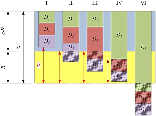
In the push–pull based ATP model, customer orders in Class 1, Class 3, and Class 5 can be fully satisfied with a remaining inventory B above the desirable reservation level R in scenario I. In scenario II, only customer orders in Class 1 and Class 3 can be fully satisfied. In contrast, a certain portion of customer orders in Class 5 has to be denied to keep the remaining inventory B at the desirable reservation level R. The situation is quite similar in scenario III that a certain portion of customer orders in Class 3 has to be denied. The remaining inventory B is below the desirable reservation level R to fulfil customer orders in Class 1 in scenario IV. Thus the entire demand in Class 3 and Class 5 is denied. In scenario IV, even customer orders in Class 1 cannot be fully satisfied. The accepted and denied volume for demand in Class 1, Class 3, and Class 5 and the remaining inventory can be summarised as follows: (1) $\begin{array}{rl}{S}_1& =\left\{\begin{array}{ll}{D}_1,& \text{if }{D}_1\le a,\\ a,& \text{if }{D}_1>a,\end{array}\right\}\end{array}$(1) (2) $\begin{array}{rl}{L}_1& =\left\{\begin{array}{ll}0,& \text{if }{D}_1\le a,\\ D_1-a,& \text{if }{D}_1>a;\end{array}\right\}\end{array}$(2) (3) $\begin{array}{rl}{S}_3& =\left\{\begin{array}{ll}{D}_3,& \text{if }{D}_1+D_3\le a-R,\\ a-R-D_1,& \begin{array}{l}\text{if }{D}_1+D_3>a-R,\\ D_1\le a-R,\end{array}\\ 0,& \text{if }{D}_1>a-R;\end{array}\right\}\end{array}$(3) (4) $\begin{array}{rl}{L}_3& =\left\{\begin{array}{ll}0,& \text{if }{D}_1+D_3\le a-R,\\ D_1+D_3-(a-R),& \begin{array}{l}\text{if }{D}_1+D_3>a-R,\\ D_1\le a-R,\end{array}\\ D_3,& \text{if }{D}_1>a-R;\end{array}\right\}\end{array}$(4) (5) $\begin{array}{rl}{S}_5& =\left\{\begin{array}{ll}{D}_5,& \text{if }{D}_1+D_3+D_5\le a-R\\ a-R-D_1-D_3,& \begin{array}{l}\text{if }{D}_1+D_3+D_5>a-R,\\ D_1+D_3\le a-R,\end{array}\\ 0,& \text{if }{D}_1+D_3>a-R;\end{array}\right\}\end{array}$(5) (6) $\begin{array}{rl}{L}_5& =\left\{\begin{array}{ll}0,& \begin{array}{l}\text{if }{D}_1+D_3\\ +D_5\le a-R\end{array}\\ \begin{array}{l}{D}_1+D_3+D_5\\ -(a-R),\end{array}& \begin{array}{l}\text{if }{D}_1+D_3+D_5\\ >a-R,\\ D_1+D_3\le a-R,\end{array}\\ D_5,& \text{if }{D}_1+D_3>a-R;\end{array}\right\}\end{array}$(6) (7) $\begin{array}{rl}B& =\left\{\begin{array}{ll}\begin{array}{l}a-D_1\\ -D_3-D_5,\end{array}& \text{if }{D}_1+D_3+D_5\le a-R,\\ R,& \begin{array}{l}\text{if }{D}_1+D_3+D_5>a-R,\\ D_1+D_3\le a-R,\end{array}\\ R,& \begin{array}{l}\text{if }{D}_1+D_3>a-R,\\ D_1\le a-R,\end{array}\\ a-D_1,& \text{if }a-R<D_1\le a,\\ 0,& \text{if }{D}_1>a\end{array}\right\}\end{array}$(7) The push–pull based ATP model can be reduced to the pull-based ATP model. Specifically, when the resource reservation level R = 0 in the push–pull based ATP model, the pull-based ATP model can be obtained. As shown in Figure 2, there are four possible demand scenarios at Stage 1 for an initial availability a in the pull-based ATP model.

• I. $D_1+D_3+D_5\le a$,

• II. $D_1+D_3+D_5>a$ and $D_1+D_3\le a$,

• III. $D_1+D_3>a$ and $D_1\le a$,

• IV. $D_1>a$.

4.2 Stage 2 ATP model

The pull-based ATP model has the same Stage 2 as the push–pull based ATP model. As shown in Figure 3, there are four possible scenarios in Stage 2:

• I. $D_2+D_4+D_6\le b$,

• II. $D_2+D_4+D_6>b$ and $D_2+D_4\le b$,

• III. $D_2+D_4>b$ and $D_2\le b$,

• IV. $D_2>b$.

Figure 2. Promising current orders in the pull-based ATP model.

In the pull-based ATP model, these are four possible demand scenarios at Stage 1 for an initial availability a without reservation.

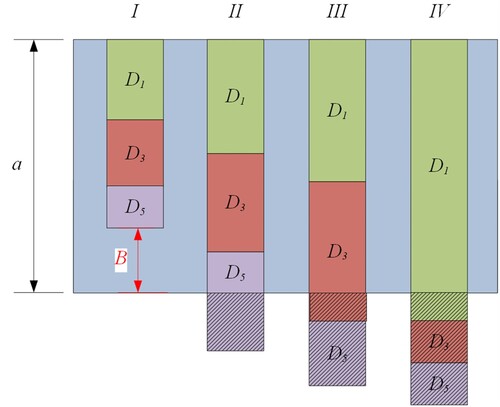
Figure 3. Promising future customer orders (with given remaining critical resource b).

In the push-pull based ATP model, there are four possible scenarios in Stage 2 for a given remaining critical resource b.

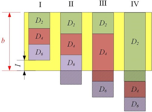
In scenario I, there exists enough remaining critical resources to fully satisfy customer orders in Class 2, Class 4, and Class 6. We can still fully satisfy customer orders in Class 2 and Class 4 but have to deny a portion of customer orders in Class 6 in scenario II. In scenario III, only demand in Class 2 can be fully satisfied, and the entire demand in Class 6 and part of demand in Class 4 is denied. There is not enough availability to fulfil customer orders in Class 2 in scenario IV. Thus the entire demand in Class 4 and Class 6 is denied. The accepted and denied volume for demand in Class 2, Class 4, and Class 6 and the remaining inventory are summarised as follows: (8) $\begin{array}{rl}{S}_2& =\left\{\begin{array}{ll}{D}_2,& \text{if }{D}_2\le b,\\ b,& \text{if }{D}_2>b;\end{array}\right\}\end{array}$(8) (9) $\begin{array}{rl}{L}_2& =\left\{\begin{array}{ll}0,& \text{if }{D}_2\le b,\\ D_2-b,& \text{if }{D}_2>b;\end{array}\right\}\end{array}$(9) (10) $\begin{array}{rl}{S}_4& =\left\{\begin{array}{ll}{D}_4,& \text{if }{D}_2+D_4\le b,\\ b-D_2,& \text{if }{D}_2+D_4>b,D_2\le b,\\ 0,& \text{if }{D}_2>b;\end{array}\right\}\end{array}$(10) (11) $\begin{array}{rl}{L}_4& =\left\{\begin{array}{l}0,\text{if }{D}_2+D_4\le b,\\ D_2+D_4-b,\text{if }{D}_2+D_4>b,D_2\le b\\ D_4,\text{if }{D}_2>b;\end{array}\right\}\end{array}$(11) (12) $\begin{array}{rl}{S}_6& =\left\{\begin{array}{ll}{D}_6,& \text{if }{D}_2+D_4+D_6\le b,\\ b-D_2-D_4,& \begin{array}{l}\text{if }{D}_2+D_4+D_6>b,\\ D_2+D_4\le b\end{array}\\ 0,& \text{if }{D}_2+D_4>b;\end{array}\right\}\end{array}$(12) (13) $\begin{array}{rl}{L}_6& =\left\{\begin{array}{ll}0,& \text{if }{D}_2+D_4+D_6\le b,\\ D_2+D_4+D_6-b,& \begin{array}{l}\text{if }{D}_2+D_4+D_6>b,\\ D_2+D_4\le b\end{array}\\ D_6,& \text{if }{D}_2+D_4>b;\end{array}\right\}\end{array}$(13) (14) $\begin{array}{rl}I& =\left\{\begin{array}{ll}b-D_2-D_4-D_6,& \text{if }{D}_2+D_4+D_6\le b,\\ 0,& \text{if }{D}_2+D_4+D_6>b;\end{array}\right\}\end{array}$(14)

4.3 Expected total profit function

For the push–pull based ATP model, the expected total profit function consists of two parts, namely the expected profit of Stage 1 and the expected profit of Stage 2 according to Equation (15). The expected profit of Stage 2 is related to the expected profit of Stage 1 through the remaining inventory B. From the above derivation, we can conclude that the expected total profit function of the pull-based ATP model is derived from the expected total profit function of the push–pull based ATP model when the reservation level R is set to zero. Since the pull-based ATP model and the push–pull based ATP model have the same derivation process, the push–pull based ATP model will be mainly discussed in the following. In the push–pull based ATP model, random variable B is determined by the reservation level R and the initial availability a, as shown in Equation (7). It is also constrained by $a-S_1-S_3-S_5=B=S_2+S_4+S_6+I$. (15) $\begin{array}{rl}& \underset{R}{max}{E}_{D_1,D_2,D_3,D_4,D_5,D_6}\left[\mathrm{\Pi }\right(a,R\left)\right]\\ & =E_{D_1,D_3,D_5}\left[{\mathrm{\Pi }}^1\right(a,R\left)\right]\\ & +E_{D_1,D_3,D_5}\left[E_{D_2,D_4,D_6}\right[{\mathrm{\Pi }}^2\left(B\right)\left]\right]\end{array}$(15) (16) $\begin{array}{rl}& E_{D_1,D_3,D_5}\left[{\mathrm{\Pi }}^1\right(a,R\left)\right]\\ & =E_{D_1,D_3,D_5}[v_1\cdot S_1+v_3\cdot S_3+v_5\cdot S_5-w_1\\ & \cdot L_1-w_3\cdot L_3-w_5\cdot L_5-g\cdot B]\\ & \text{ = }{v}_1\cdot E\left[S_1\right]+v_3\cdot E\left[S_3\right]+v_5\cdot E\left[S_5\right]-w_1\cdot E\left[L_1\right]\\ & -w_3\cdot E\left[L_3\right]-w_5\cdot E\left[L_5\right]-g\cdot E\left[B\right]\end{array}$(16) (17) $\begin{array}{rl}& E_{D_2,D_4,D_6}\left[{\mathrm{\Pi }}^2\right(B\left)\right]\\ & =E_{D_2,D_4,D_6}[v_2\cdot S_2+v_4\cdot S_4+v_6\cdot S_6-w_2\cdot L_2\\ & -w_4\cdot L_4-w_6\cdot L_6-h\cdot I]\\ & \text{ = }{v}_2\cdot E\left[S_2\right]+v_4\cdot E\left[S_4\right]+v_6\cdot E\left[S_6\right]-w_2\cdot E\left[L_2\right]\\ & -w_4\cdot E\left[L_4\right]-w_6\cdot E\left[L_6\right]-h\cdot E\left[I\right]\end{array}$(17)

To obtain the expected profit of Stage 1, the expected value of accepted and denied volume for demand in Class 1, Class 3, and Class 5 and the remaining inventory need to be derived as follows: (18) $\begin{array}{rl}E\left[S_1\right]& =Pr\{D_1\le a\}\cdot D_1+Pr\{D_1>a\}\cdot a\end{array}$(18) (19) $\begin{array}{rl}E\left[S_3\right]& =Pr\{D_1+D_3\le a-R\}\cdot D_3\\ & +Pr\{D_1+D_3>a-R\}\\ & \cdot Pr\{D_1\le a-R\}\cdot (a-R-D_1)\end{array}$(19) (20) $\begin{array}{rl}E\left[S_5\right]& =Pr\{D_1+D_3+D_5\le a-R\}\cdot D_5\\ & +Pr\{D_1+D_3+D_5>a-R\}\\ & \cdot Pr\{D_1+D_3\le a-R\}\cdot (a-R-D_1-D_3)\end{array}$(20) (21) $\begin{array}{rl}E\left[L_1\right]& =Pr\{D_1>a\}\cdot (D_1-a)\end{array}$(21) (22) $\begin{array}{rl}E\left[L_3\right]& =Pr\{D_1+D_3>a-R\}\\ & \cdot Pr\{D_1\le a-R\}\cdot (D_1+D_3-a+R)\\ & +Pr\{D_1>a-R\}\cdot D_3\end{array}$(22) (23) $\begin{array}{rl}E\left[L_5\right]& =Pr\{D_1+D_3+D_5>a-R\}\\ & \cdot Pr\{D_1+D_3\le a-R\}\\ & \cdot (D_1+D_3+D_5-a+R)\\ & +Pr\{D_1+D_3>a-R\}\cdot D_5\end{array}$(23) (24) $\begin{array}{rl}E\left[B\right]& =Pr\{D_1+D_3+D_5\le a-R\}\\ & \cdot (a-D_1-D_3-D_5)\\ & +Pr\{D_1+D_3+D_5>a-R\}\\ & \cdot Pr\{D_1+D_3\le a-R\}\cdot R\\ & +Pr\{D_1+D_3>a-R\}\cdot Pr\{D_1\le a-R\}\cdot R\\ & +Pr\{a-R<D{}_1\le a\}\cdot (a-D_1)\end{array}$(24) By plugging Equations (18)-(24) into Equation (16), the expected profit of Stage 1 is derived.

Since the expected profit of Stage 2 is related to the remaining inventory B, thus the expected profit of Stage 2 should be calculated comprehensively with different remaining inventory in different scenarios. (25) $\begin{array}{rl}& E_{D_1,D_3,D_5}\left[E_{D_2,D_4,D_6}\right[{\mathrm{\Pi }}^2\left(B\right)\left]\right]\\ & =\text{Pr}\{D_1+D_3+D_5\le a-R\}\\ & \cdot E_{D_2,D_4,D_6}\left[{\mathrm{\Pi }}^2\right(B\left)\right]|{}_{B=a-D_1-D_3-D_5}\\ & +[Pr\{D_1+D_3+D_5>a-R\}\\ & \cdot Pr\{D_1+D_3\le a-R\}\\ & +Pr\{D_1+D_3>a-R\}\cdot Pr\{D_1\le a-R\}]\\ & \cdot E_{D_2,D_4,D_6}\left[{\mathrm{\Pi }}^2\right(B\left)\right]|{}_{B=R}\\ & +Pr\{a-R<D_1\le a\}\cdot E_{D_2,D_4,D_6}\left[{\mathrm{\Pi }}^2\right(B\left)\right]|{}_{B=a-D_1}\\ & +Pr\{D_1>a\}\cdot E_{D_2,D_4,D_6}\left[{\mathrm{\Pi }}^2\right(B\left)\right]|{}_{B=0}\end{array}$(25) To obtain the expected profit of Stage 2 with random variable B, the expected value of accepted and denied volume for demand in Class 2, Class 4 and Class 6 and the remaining inventory need to be derived as follows: (26) $\begin{array}{rl}E\left[S_2\right]& =Pr\{D_2\le B\}\cdot D_2+Pr\{D_2>B\}\cdot B\end{array}$(26) (27) $\begin{array}{rl}E\left[S_4\right]& =Pr\{D_2+D_4\le B\}\cdot D_4+Pr\{D_2+D_4>B\}\\ & \cdot Pr\{D_2\le B\}\cdot (B-D_2)\end{array}$(27) (28) $\begin{array}{rl}E\left[S_6\right]& =Pr\{D_2+D_4+D_6\le B\}\cdot D_6\\ & +Pr\{D_2+D_4+D_6>B\}\\ & \cdot Pr\{D_2+D_4\le B\}\cdot (B-D_2-D_4)\end{array}$(28) (29) $\begin{array}{rl}E\left[L_2\right]& =Pr\{D_2>B\}\cdot (D_2-B)\end{array}$(29) (30) $\begin{array}{rl}E\left[L_4\right]& =Pr\{D_2+D_4>B\}\cdot Pr\{D_2\le B\}\\ & \cdot (D_2+D_4-B)+Pr\{D_2>B\}\cdot D_4\end{array}$(30) (31) $\begin{array}{rl}E\left[L_6\right]& =Pr\{D_2+D_4+D_6>B\}\cdot Pr\{D_2+D_4\le B\}\\ & \cdot (D_2+D_4+D_6-B)\\ & +Pr\{D_2+D_4>B\}\cdot D_6\end{array}$(31) (32) $\begin{array}{rl}E\left[I\right]& =Pr\{D_2+D_4+D_6\le B\}\cdot (B-D_2-D_4-D_6)\end{array}$(32)

By plugging Equations (26)-(32) into Equation (17), and subsequently, plugging Equation (17) with different values B into Equation (25), the expected profit of Stage 2 is derived.

Then the optimal reservation level R* must satisfy the Equation (33): (33) $\begin{array}{rl}& -(v_3+w_3+g)\cdot Pr\{D_1+D_3>a-R^{\ast }\}\\ & \cdot Pr\{D_1\le a-R^{\ast }\}\\ & -(v_5+w_5+g)\cdot Pr\{D_1+D_3+D_5>a-R^{\ast }\}\\ & \cdot Pr\{D_1+D_3\le a-R^{\ast }\}\\ & +[Pr\{D_1+D_3>a-R^{\ast }\}\\ & \cdot Pr\{D_1\le a-R^{\ast }\}\\ & +Pr\{D_1+D_3+D_5>a-R^{\ast }\}\\ & \cdot Pr\{D_1+D_3\le a-R^{\ast }\}]\\ & \cdot [Pr\{D_2>R^{\ast }\}\cdot (v_2+w_2)+Pr\{D_2+D_4>R^{\ast }\}\\ & \cdot Pr\{D_2\le R^{\ast }\}\cdot (v_4+w_4)\\ & +Pr\{D_2+D_4+D_6>R^{\ast }\}\\ & \cdot Pr\{D_2+D_4\le R^{\ast }\}\cdot (v_6+w_6)\\ & -h\cdot Pr\{D_2+D_4+D_6\le R^{\ast }\}]=0\end{array}$(33) To prove the expected total profit function is concave, the second derivative of the expected total profit should be proven to be negative when evaluated at R*. Thus, the second derivative of the expected total profit function is derived as follows: (34) $\begin{array}{rl}\frac{d^{2}E[\prod (R^{\ast }\left)\right]}{d{R}^2}& =\left[\right(v_2+w_2)\cdot \frac{d}{dR}Pr\{D_2>R^{\ast }\}\\ & +(v_4+w_4)\\ & \cdot \frac{d}{dR}Pr\{D_2+D_4>R^{\ast },D_2\le R^{\ast }\}\\ & +(v_6+w_6)\\ & \cdot \frac{d}{dR}Pr\{D_2+D_4+D_6>R^{\ast },\\ & D_2+D_4\le R^{\ast }\}\\ & -h\cdot \frac{d}{dR}Pr\{D_2+D_4+D_6\le R^{\ast }\}]\\ & \cdot [Pr\{D_1+D_3>a-R\}\\ & \cdot Pr\{D_1\le a-R\}\\ & +Pr\{D_1+D_3+D_5>a-R\}\\ & \cdot Pr\{D_1+D_3\le a-R\}]\\ & =-\left[\right(v_2+w_2)\cdot f_2(R^{\ast })\\ & +(v_4+w_4)\cdot f_4\left(R^{\ast }\right)\\ & +(v_6+w_6+h)\\ & \cdot \underset{0}{\overset{R^{\ast }}{\int }}{f}_6(R^{\ast }-x-y)d{F}_2\left(x\right)d{F}_2\left(y\right)]\\ & \cdot [Pr\{D_1+D_3>a-R\}\\ & \cdot Pr\{D_1\le a-R\}\\ & +Pr\{D_1+D_3+D_5>a-R\}\\ & \cdot Pr\{D_1+D_3\le a-R\}]<0\end{array}$(34) Therefore, an optimal reservation level R* exists, which can maximise the expected total profit function. It should be noted that the optimal reservation level cannot be obtained explicitly by Equation (33).

5 Numerical experiments

This section presents a series of available-to-promise computations to verify the validity of this dynamic resource reservation policy where the optimal reservation level R* can maximise the expected total profit. Numerical examples are provided to highlight the benefit of a dynamic resource reservation policy by comparing the optimal profit of the pull-based ATP model with that of the push–pull based ATP model. Besides, computational results are analysed to show the sensitivity of each altered input parameter, which will help enterprises make business decisions on order management.

5.1 Genetic algorithm

Although we have derived the implicit expression of the optimal reservation level R* and theoretically proved the existence and uniqueness of the optimal reservation level, this does not necessarily mean that we can obtain the optimal reservation level explicitly by Equation (33). Since the objective function is stochastic, standard optimisation algorithms are not well suited for solving this problem. Therefore the genetic algorithm (GA) is a promising tool to find the optimal reservation level. GA is an iterative optimisation method based on natural selection, which repeatedly modifies a population of individual solutions to make the population evolve toward an optimal solution over successive iterations (Lim 2014).

The basic modules of GA consist of 1) encoding and decoding, 2) fitness function, 3) selection, mutation, and crossover. In this paper, a real-coded genetic algorithm is used, and the fitness function is $T_{MAX}-E_{D_1,D_2,D_3,D_4,D_5,D_6}\left[\mathrm{\Pi }\right(a,R\left)\right]$, where T_MAX is a sufficiently large constant to ensure that the fitness function keeps positive. Roulette selection, Scattered crossover, and Gaussian mutation are used respectively in this study.

5.2 Numerical examples

Table 2 provides the basic parameters of these six demand classes. Only taking sales prices and component costs into account without charging any production and operation costs, we assume the profit margins v₁, v₂, v₃, v₄, v_5, and v₆ to be 940, 846, 761, 685, 616, and 555 CNY respectively. While the per-unit denial penalty cost is assumed to be ten per cent of the profit margin, per-unit inventory holding costs for the critical resources are assumed to be fixed. That is g, h = 3.25 CNY. Suppose all demands are normally distributed and independent, and their corresponding mean value μ_i and standard deviation σ_i are given in Table 2. The initial availability for the critical resource comes to be 5,730 units.

Table 2. Characteristics of Demand Classes

Order	Profit Margin
Stage	High Profit	Medium Profit	Low Profit
Stage 1 (current actual)	$v_1=940$CNY	$v_3=761$CNY	$v_5=616$CNY
	$w_1=94$CNY	$w_3=76$CNY	$w_5=61$CNY
	$\mu {}_1=1474$ units	${\mu }_3=1783$ units	${\mu }_5=2157$ units
	${\sigma }_1=85.6$ units	${\sigma }_3=103.5$ units	${\sigma }_5=125.1$ units
Stage 2 (future forecast)	$v_2=846$CNY	$v_4=685$CNY	$v_6=555$CNY
	$w_2=85$CNY	$w_4=68$CNY	$w_6=55$CNY
	${\mu }_2=1621$ units	${\mu }_4=1961$ units	${\mu }_6=2372$ units
	${\sigma }_2=94.1$ units	${\sigma }_4=113.8$ units	${\sigma }_6=137.6$ units

A simulation model that implements the dynamic reservation policy is built to conduct the numerical experiments by MATLAB. The experiment computes the average total profit over 1000 sets of randomly generated demands D₁, D₂, D₃, D₄, D_5, and D₆ for each pair of the reservation level to see whether the optimal reservation level derived by the genetic algorithm can maximise the total profit.

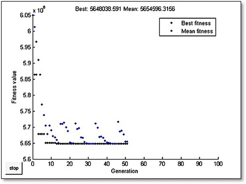
Take $T_{MAX}=10,000,000$, GA stops at the 51st generation, as shown in Figure 4. The optimal reservation level R* turns out to be 2463 units, and the corresponding maximal expected total profit is 4,352,000 CNY. However, the maximal expected total profit is only 3,963,500 CNY under the pull-based ATP model. This verifies that the push–pull based ATP model is significantly superior to the pull-based ATP model and also demonstrates the necessity and effectiveness of introducing the forecast demand information and dynamic resource reservation policy into the pull-based ATP model.

Figure 4. Best fitness value in each generation versus iteration number.

GA stops at the 51st generation, the optimal reservation level R* turns out to be 2463 units, and the corresponding maximal expected total profit is 4352000 CNY.

5.3 Computational results

This section explores the impact of some key factors on expected/average total profit, including resource reservation level, initial availability, denial penalty cost, inventory holding cost, and future pricing level. The experiment results provide theoretical guidance and implementation methods for companies to maximise overall profits.

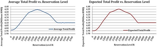
5.3.1 Impact of resource reservation level

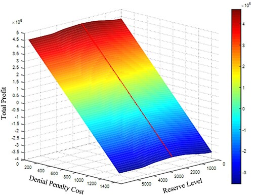
Figure 5 shows the impact of different reservation levels on the expected total profit and the average total profit, respectively. As shown in Figure 5, there exists a maximal total profit in both figures, the maximal total profit is around 4,352,000 CNY, and the corresponding reservation level is around 2460 units. Thus, the optimal reservation level derived by GA can be considered the optimum solution. It can also be deduced from Figure 5 that the total profit rises with the increasing reservation level till its peak value and then falls to a certain level because the critical resource is reserved to satisfy more profitable future customer orders that result in higher profitability. Still, if the reservation amount is set at an unreasonably high level, total profit will stay the same since all the customer orders in Class 3 and Class 5 are denied after fully fulfilling customer orders in Class 1, with the same amounts of remaining critical resources.

Figure 5. Impact of dynamic resource reservation policy.

It reflects the impact of different reservation levels on the expected total profit and the average total profit and shows that the total profit rises with the increasing reservation level till its peak value and then falls to a certain level.

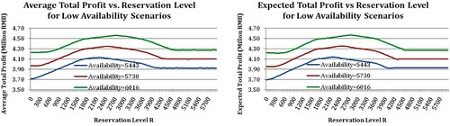
5.3.2 Impact of initial availability

When investigating the impact of initial availability on the optimal reservation level, three initial availability values are tested, including the base-scenario value and its$\pm$5% values (i.e. 5443, 5730, and 6016 units). Figure 6 shows that the optimal reservation level experiences an increasing trend due to increasing availability. Since the extra critical resource will be reserved for customer orders in Class 4 rather than pre-allocated to customer orders in Class 5 to ensure maximal profit.

Figure 6. Impact of initial availability on reservation level (for low availability scenarios).

It reflects the different reservation levels on the expected total profit and the average total profit under three low initial availability scenarios and shows that the optimal reservation level experiences an increasing trend due to increasing availability.

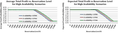
Similarly, we run the experiment with another three availability values around the mean total demand (i.e. 11,586, 11,966, and 12,346 units). As shown in Figure 7, a dynamic resource reservation policy becomes less important when there are abundant critical resources. Besides, if the reservation level is set very high, the total profit will be damaged, resulting in the rejection of customer orders in Class 3 and Class 5.

Figure 7. Impact of initial availability on reservation level (for high availability scenarios).

It reflects the different reservation levels on the expected total profit and the average total profit under three high initial availability scenarios and shows that the proposed dynamic resource reservation policy becomes less important when there are abundant critical resources.

5.3.3 Impact of denial penalty cost

The per-unit denial penalty cost is set into different ratio levels of the per-unit profit to reveal the impact of denial penalty cost while combining dynamic resource reservation policy. Since changes in per-unit denial penalty cost may affect the reserve police of those three classes in Stage 1, the optimal reservation level may need to adjust adaptively. A set of ratio levels are chosen at regular intervals from 0 to 1.5. Figure 8 shows that the optimal reservation level experiences little change, and the optimal price level stays around R* = 2461 CNY which maximises the overall profit when combining dynamic resource reservation policy. The main reason for this is that these six per-unit denial penalty costs are changed in the same proportion, and the priority used to determine the reservation level is not changed. The same thing happens when the per-unit denial penalty cost of these six classes is set at the same value. The values of per-unit denial penalty cost are chosen at regular intervals from 0 to 1200, while all the other parameters are the same as those in Table 2. As shown in Figure 9, the optimal reservation level still experiences little change, and the corresponding reservation level stays around 2461 units. One possible reason is that the differences between these six per-unit profits determine the relative priority, and the fluctuation of the same per-unit denial penalty cost does not change it.

Figure 8. Impact of per-unit denial penalty cost of different ratio levels on reservation level.

Under different ratio levels of per-unit denial penalty cost, the optimal reservation level experiences little change, and the optimal price level stays around 2461 units.

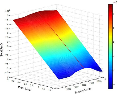
Figure 9. Impact of per-unit denial penalty cost with the same value on the reservation level.

Under different per-unit denial penalty costs, the optimal reservation level still experiences little change, and the corresponding reservation level stays around 2461 units.

Another two experiments are conducted to study further the impact of per-unit denial penalty cost on reservation level. In the first experiment, the values of the per-unit denial penalty cost of Class 1 are chosen at regular intervals from 0 to 1000, with all other parameters the same as those in Table 2. As shown in Figure 10, the optimal reservation level still experiences little change, and the corresponding reservation level stays around 2461 units. The main reason is that whatever the per-unit denial penalty cost of Class 1, the critical resources are used to satisfy the demand of Class 1 for the highest per-unit profit. In the second experiment, the values of the per-unit denial penalty cost of both Class 1 and Class 2 are chosen at regular intervals from 0 to 1000, with all other parameters the same as those in Table 2. Figure 11 shows that the optimal reserve level is volatile within a very small range when w₁ and w₂ are set to different values. Except for the random factors, the change of relative priority between Class 1 and Class 2 is also an important cause.

Figure 10. Impact of per-unit denial penalty cost of class 1 on reservation level.

Under different per-unit denial penalty cost w1, the optimal reservation level still experiences little change, and the corresponding reservation level stays around 2461 units.

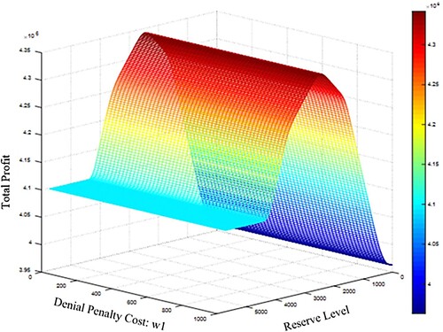
Figure 11. Impact of per-unit denial penalty cost of both class 1 and class 2 on reservation level.

The optimal reserve level is volatile within a very small range when per-unit denial penalty cost w1 and w2 are set to different values.

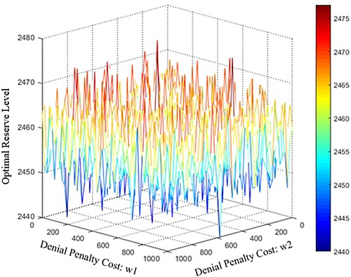
It is a remarkable fact that the optimal reservation level remains stable when the per-unit denial penalty cost of these six classes is set at the same ratio level or the same value. Only when multiple unit penalty costs are changed together, the optimal reserve level may present obvious fluctuation.

5.3.4 Impact of inventory holding cost

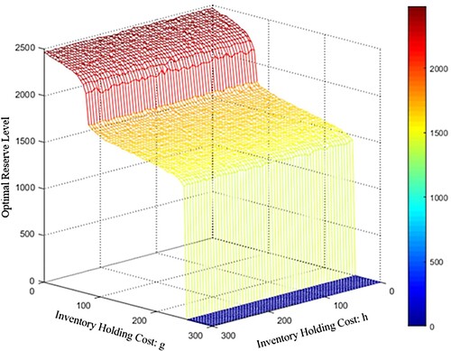
The per-unit inventory holding costs for the critical resources are set into different value to reveal the impact of inventory holding costs while combining dynamic resource reservation policy. The values of per-unit component inventory holding cost g and h are chosen at regular intervals from 0 to 300, with all the other parameters the same as those in Table 2. From Figure 12, it can be seen that when the per-unit component inventory cost g is fixed, the optimal reserve level has a very small fluctuation with the change of the per-unit component inventory cost h, whereas, when h is fixed, the optimal reservation level experiences a step down with the growth of g. The root cause is quite likely that the final inventory is relatively certain, so the impact of per-unit component inventory cost h at the end of Stage 2 is relatively small when g is fixed. Moreover, when h is fixed, the value of g could determine that the critical resource is offered to Class 3 and Class 5, or left for Stage 2.

Figure 12. Impact of inventory holding cost g and h on reservation level.

When the per-unit component inventory cost g is fixed, the optimal reserve level has a very small fluctuation with the change of the per-unit component inventory cost h, whereas, when h is fixed, the optimal reservation level experiences a step down with the growth of g.

5.3.5 Impact of future pricing level

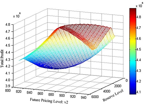
The per-unit sales profit of customer orders in Class 2 is set at a different level to reveal the impact of future pricing levels while combining dynamic resource reservation policy. Since price changes will affect the demand in different Classes, for instance, the rising price in Class 2 will reduce the demand in Class 2. Assume the demand-price elasticity$\mathrm{\partial }$ for Class 2 customer orders is −40 units per CNY, thus${\mu }_2={\mu }_1-\mathrm{\partial }(940-v_2)$, while all the other parameters are the same as those in Table 2. As shown in Figure 13, the optimal price level v2 = 885 CNY exists, which maximises the total profit when combining a dynamic resource reservation policy. Furthermore, Figure 14 clearly shows the total profit under each combination of future pricing level and reservation level. Figure 13 can be seen as a projection of Figure 14 on the plane of total profit and future pricing level. Besides, it can be seen from Figure 14 that the optimal reservation level shows a noticeable trend of growth with the reduction of future pricing levels. Since the extra critical resource will be reserved for customer orders in Class 2 due to the increasing demand caused by lower prices, the maximum total profit can be achieved if the manufacturer sets a proper price and combines the dynamic resource reservation policy. Thus a combination of dynamic pricing policy and dynamic resource reservation policy on different classes can be future research.

Figure 13. Impact of future pricing level on the total profit.

The optimal price level v2 = 885 CNY exists, maximising the total profit when combining dynamic resource reservation policy.

Figure 14. Impact of future pricing level on the reservation level and total profit.

The optimal reservation level shows an obvious growing trend with the reduction of future pricing levels.

6 Conclusions

This study proposes a push–pull based ATP stochastic model that takes into account potential future customer demands and develops a dynamic resource reservation policy for a push–pull based ATP problem with two time stages and three profit margin levels. This policy maximises the expected total profit by enforcing a reservation level and preventing current less-profitable customer orders from over-consuming critical resources. A real-coded genetic algorithm is introduced to solve the corresponding stochastic model and derive the optimal reservation level. A series of numerical experiments are conducted to reveal important managerial insights of this policy. The simulation experiments revealed that the push–pull based ATP model is significantly superior to the pull-based ATP model, demonstrating the necessity and effectiveness of introducing the forecast demand information and dynamic resource reservation policy into the pull-based ATP model. Besides, the total profit rises with the increase of the reservation level until it reaches the peak value and then falls to a certain level. The optimal reservation level is positively correlated to initial availability in low availability scenarios and is insensitive to the initial availability in high availability scenarios. Moreover, different parameter combinations of per-unit denial penalty costs of these six classes and per-unit component inventory holding costs are also explored to disclose the functional mechanism of the optimal reserve level of these parameters. Finally, the impact of future pricing levels on the optimal reserve level is discussed. The study makes an important contribution to the overall knowledge of the ATP model. From another point of view, the development of the push–pull based ATP model also greatly promotes the application of information forecasting in the ATP model.

Although the research has addressed several academically challenging issues, it has a few limitations when applying the policy to real-world ATP systems, which will be studied in future work. First, it did not explore how to assign customer demand space into different classes, which is a critical research question and requires more research to look into appropriate criteria for separating customer demand space so that the expected total profit can be maximised efficiently. Second, it did not involve how to forecast corresponding demand distributions, which is a crucial step in executing the push–pull based ATP model since the appropriateness of optimal reservation level and optimal pricing level is directly tied to the quality of forecasted demand distributions. Third, the combination of a dynamic pricing policy and dynamic resource reservation policy is promising to achieve the highest total profit. Besides, enlarging the ATP model into more customer groups and demand stages will help the policy available for larger ATP problems.

Data availability statement

The data that support the findings of this study are available from the corresponding authors, W.Q. and Y. L., upon reasonable request.

Acknowledgements

The authors would like to acknowledge the financial support of the National Natural Science Foundation of China (No. 51775348).

Disclosure statement

No potential conflict of interest was reported by the author(s).

Additional information

Notes on contributors

Wei Qin

Wei Qin received the B.S. degree in ship and ocean engineering from Shanghai Jiao Tong University, Shanghai, China, in 2004 and the M.S. degree in automation from Tsinghua University, Beijing, China, in 2006. And in 2011, he received his Ph.D. degree in industrial and manufacturing systems engineering from the University of Hong Kong, Hong Kong, China. He is currently an Associate Professor and the Associate Head of the Department of Industrial Engineering at the School of Mechanical Engineering, Shanghai Jiao Tong University, Shanghai, China. His current research interests include modeling, control, and optimisation of complex systems, machine intelligence, and smart manufacturing. He has authored/co-authored over thirty research papers in refereed international journals and conferences and has been serving as a reviewer for many top-tier international journals and conferences in his research field.

Zilong Zhuang

Zilong Zhuang received the B.S. degree from Beihang University, China, in 2016, and the Ph.D. degree from Shanghai Jiao Tong University, China, in 2021. He is currently an algorithm researcher at Shanghai Huawei Technology Co. Ltd. His current research interests include machine learning, operations research, and their applications in smart manufacturing.

Yanning Sun

Yanning Sun received the B.S. degree in mechanical engineering and automation from Northeastern University at Qinhuangdao, Qinhuangdao, China, in 2016 and the M.S. degree in mechanical design and theory from Northeastern University, Shenyang, China, in 2019. He is currently pursuing the Ph.D. degree in mechanical engineering at Shanghai Jiao Tong University, Shanghai, China. His current research interests include the fundamental study of artificial intelligence, complex network and industrial systems, data-driven decision-making methods in complex industrial processes, and development of industrial big data platform for intelligent manufacturing.

Yang Liu

Yang Liu received his M.Sc. (Tech.) degree in telecommunication engineering and D.Sc. (Tech.) degree in industrial management from the University of Vaasa, Finland, in 2005 and 2010, respectively. He is currently a tenured Associate Professor with the Department of Management and Engineering, Linköping University, Sweden, and an Adjunct Professor with the Industrial Engineering and Management, University of Oulu, Finland. His research interests include sustainable smart manufacturing, product service innovation, decision support system, competitive advantage, control systems, autonomous robots, signal processing, and pattern recognition. Prof. Liu has authored/co-authored over 110 Web of Science indexed publications. He is ranked No.1 among the top authors on ‘big data analytics in manufacturing', and among the top 1% scientists in Engineering and Technology by Research.com. His publications have appeared in multiple distinguished journals, and some ranked in the top 0.1% ESI Hot Papers and top 1% ESI Highly Cited Papers. He serves as an Associate Editor of the prestigious Journal of Cleaner Production and Journal of Intelligent Manufacturing.

Miying Yang

Miying Yang is a Reader in Sustainability at the Cranfield University. She holds a PhD degree from the Centre for Industrial Sustainability at the University of Cambridge (2011-2015), worked as a postdoc in Sustainable Manufacturing at Cranfield University (2016), and was a lecturer and subsequently senior lecturer at the University of Exeter (2017-2021). She was a visiting scholar at Stanford University (2018). Her recent work focuses on how to make manufacturing and supply chain more sustainable through digitalisation and business model innovation. She developed a Sustainable Value Analysis Tool which helped over 100 firms identify their sustainable value opportunities.

Appendix 1

Derivation of Equation (33) $\frac{dE\left[\mathrm{\Pi }\right(a,R\left)\right]}{dR}=\frac{dE\left[{\mathrm{\Pi }}^1\right(a,R\left)\right]}{dR}+\frac{dE\left[E\right[{\mathrm{\Pi }}^2\left(B\right)\left]\right]}{dR}$Start with differentiating the expected profit of Stage 1 for R, $\begin{array}{rl}\frac{dE\left[\prod ^1\right(a,R\left)\right]}{dR}& =-(v_3+w_3+g)\cdot Pr\{D_1+D_3>a-R\}\\ & \cdot Pr\{D_1\le a-R\}\\ & -(v_5+w_5+g)\\ & \cdot Pr\{D_1+D_3+D_5>a-R\}\\ & \cdot Pr\{D_1+D_3\le a-R\}\end{array}$Next is the derivative of the expected profit of Stage 2 for R, $\begin{array}{rl}\frac{dE\left[E\right[\prod ^2\left(B\right)\left]\right]}{dR}& =[Pr\{D_1+D_3>a-R\}\cdot Pr\{D_1\le a-R\}\\ & +Pr\{D_1+D_3+D_5>a-R\}\\ & \cdot Pr\{D_1+D_3\le a-R\}]\\ & \cdot \frac{d{E}_{D_2,D_4,D_6}\left[\prod ^2\right(R\left)\right]}{dR}\end{array}$where $\begin{array}{rl}& \frac{d{E}_{D_2,D_4,D_6}\left[\prod ^2\right(B\left)\right]}{dB}{|}_{B=R}\\ & =Pr\{D_2>R\}\cdot (v_2+w_2)+Pr\{D_2+D_4>R\}\\ & \cdot Pr\{D_2\le R\}\cdot (v_4+w_4)\\ & +Pr\{D_2+D_4+D_6>R\}\\ & \cdot Pr\{D_2+D_4\le R\}\cdot (v_6+w_6)\\ & -h\cdot Pr\{D_2+D_4+D_6\le R\}\end{array}$Thus, when $\frac{dE\left[\mathrm{\Pi }\right(a,R\left)\right]}{dR}=0$, the optimal reservation level R* must satisfy the Equation below: $\begin{array}{rl}& -(v_3+w_3+g)\cdot Pr\{D_1+D_3>a-R^{\ast }\}\cdot Pr\{D_1\le a-R^{\ast }\}\\ & -(v_5+w_5+g)\cdot Pr\{D_1+D_3+D_5>a-R^{\ast }\}\\ & \cdot Pr\{D_1+D_3\le a-R^{\ast }\}\\ & +[Pr\{D_1+D_3>a-R^{\ast }\}\cdot Pr\{D_1\le a-R^{\ast }\}\\ & +Pr\{D_1+D_3+D_5>a-R^{\ast }\}\cdot Pr\{D_1+D_3\le a-R^{\ast }\}]\\ & \cdot [Pr\{D_2>R^{\ast }\}\cdot (v_2+w_2)+Pr\{D_2+D_4>R^{\ast }\}\\ & \cdot Pr\{D_2\le R^{\ast }\}\cdot (v_4+w_4)\\ & +Pr\{D_2+D_4+D_6>R^{\ast }\}\\ & \cdot Pr\{D_2+D_4\le R^{\ast }\}\cdot (v_6+w_6)\\ & -h\cdot Pr\{D_2+D_4+D_6\le R^{\ast }\}]=0\end{array}$Derivation of Equation (34)

To prove the expected total profit function is concave, the second derivative of the expected total profit should be proven to be negative when evaluated at R*. $\frac{d^{2}E\left[\mathrm{\Pi }\right(a,R^{\ast }\left)\right]}{d{R}^2}=\frac{d^{2}E\left[{\mathrm{\Pi }}^1\right(a,R^{\ast }\left)\right]}{d{R}^2}+\frac{d^{2}E\left[E\right[{\mathrm{\Pi }}^2\left(B\right)\left]\right]}{d{R}^2}<0$Thus, the second derivative of the expected total profit function is derived as follows: $\begin{array}{rl}\frac{d^{2}E[\prod (R^{\ast }\left)\right]}{d{R}^2}& =\left[\right(v_2+w_2)\cdot \frac{d}{dR}Pr\{D_2>R^{\ast }\}\\ & +(v_4+w_4)\\ & \cdot \frac{d}{dR}Pr\{D_2+D_4>R^{\ast },D_2\le R^{\ast }\}\\ & +(v_6+w_6)\\ & \cdot \frac{d}{dR}Pr\{D_2+D_4+D_6>R^{\ast },D_2+D_4\le R^{\ast }\}\\ & -h\cdot \frac{d}{dR}Pr\{D_2+D_4+D_6\le R^{\ast }\}]\\ & \cdot [Pr\{D_1+D_3>a-R^{\ast }\}\cdot Pr\{D_1\le a-R^{\ast }\}\\ & +Pr\{D_1+D_3+D_5>a-R^{\ast }\}\\ & \cdot Pr\{D_1+D_3\le a-R^{\ast }\}]\end{array}$Then $\begin{array}{rl}\frac{d^{2}E[\prod (R^{\ast }\left)\right]}{d{R}^2}& =-\left[\right(v_2+w_2)\cdot f_2(R^{\ast })+(v_4+w_4)\cdot f_4(R^{\ast })\\ & +(v_6+w_6+h)\\ & \cdot \underset{0}{\overset{R^{\ast }}{\int }}{f}_6(R^{\ast }-x-y)d{F}_2\left(x\right)d{F}_2\left(y\right)]\\ & \cdot [Pr\{D_1+D_3>a-R^{\ast }\}\cdot Pr\{D_1\le a-R^{\ast }\}\\ & +Pr\{D_1+D_3+D_5>a-R^{\ast }\}\\ & \cdot Pr\{D_1+D_3\le a-R^{\ast }\}]<0\end{array}$Therefore, an optimal reservation level R* exists^, which can maximise the expected total profit function.

References

- Abedi, A., and W. Zhu. 2020. “An Advanced Order Acceptance Model for Hybrid Production Strategy.” Journal of Manufacturing Systems 55: 82–93. doi:10.1016/j.jmsy.2020.02.012
- Alemany, M. M. E., H. Grillo, A. Ortiz, and V. S. Fuertes-Miquel. 2015. “A Fuzzy Model for Shortage Planning Under Uncertainty due to Lack of Homogeneity in Planned Production Lots.” Applied Mathematical Modelling 39 (15): 4463–4481. doi:10.1016/j.apm.2014.12.057
- Ball, M. O., C. Y. Chen, and Z. Y. Zhao. 2004. “Handbook of Quantitative Supply Chain Analysis.” Springer US.
- Buergin, J., A. Hammerschmidt, H. Hao, S. Kramer, H. Tutsch, and G. Lanza. 2019. “Robust Order Planning with Planned Orders for Multi-Variant Series Production in a Production Network.” International Journal of Production Economics 210: 107–119. doi:10.1016/j.ijpe.2019.01.013
- Cano-Belmán, J., and H. Meyr. 2019. “Deterministic Allocation Models for Multi-Period Demand Fulfillment in Multi-Stage Customer Hierarchies.” Computers & Operations Research 101: 76–92. doi:10.1016/j.cor.2018.09.002
- Chen, C. Y., Z. Y. Zhao, and M. O. Ball. 2002. “A Model for Batch Advanced Available-to-Promise.” Production and Operations Management 11: 424–440. doi:10.1111/j.1937-5956.2002.tb00470.x
- Dumetz, L., J. Gaudreault, A. Thomas, N. Lehoux, P. Marier, and H. El-Haouzi. 2017. “Evaluating Order Acceptance Policies for Divergent Production Systems with co-Production.” International Journal of Production Research 55 (13): 3631–3643. doi:10.1080/00207543.2016.1193250
- Ervolina, T. R., M. Ettl, Y. M. Lee, and D. J. Peters. 2009. “Managing Product Availability in an Assemble-to-Order Supply Chain with Multiple Customer Segments.” OR Spectrum 31: 257–280. doi:10.1007/s00291-007-0113-4
- Esteso, A., J. Mula, F. Campuzano-Bolarín, M. A. Diaz, and A. Ortiz. 2019. “Simulation to Reallocate Supply to Committed Orders Under Shortage.” International Journal of Production Research 57 (5): 1552–1570. doi:10.1080/00207543.2018.1493239
- Fleischmann, M., K. Kloos, M. Nouri, and R. Pibernik. 2020. “Single-period Stochastic Demand Fulfillment in Customer Hierarchies.” European Journal of Operational Research 286 (1): 250–266. doi:10.1016/j.ejor.2020.03.030
- Framinan, J. M., and R. Leisten. 2010. “Available-to-promise (ATP) Systems: A Classification and Framework for Analysis.” International Journal of Production Research 48 (11): 3079–3103. doi:10.1080/00207540902810544
- Gao, L., S. H. Xu, and M. O. Ball. 2012. “Managing an Available-to-Promise Assembly System with Dynamic Short-Term Pseudo-Order Forecast.” Management Science 58 (4): 770–790. doi:10.1287/mnsc.1110.1442
- Hariharan, R., and P. Zipkin. 1995. “Customer-order Information, Lead-Times, and Inventories.” Management Science 41 (10): 1599–1607. doi:10.1287/mnsc.41.10.1599
- Hempsch, C., H. J. Sebastian, and T. Bui. 2013. “Solving the Order Promising Impasse Using Multi-Criteria Decision Analysis and Negotiation.” Logistics Research 6 (1): 25–41. doi:10.1007/s12159-012-0094-9
- Hu, X., G. Wang, X. Li, Y. Zhang, S. Feng, and A. Yang. 2018. “Joint Decision Model of Supplier Selection and Order Allocation for the Mass Customization of Logistics Services.” Transportation Research Part E: Logistics and Transportation Review 120: 76–95. doi:10.1016/j.tre.2018.10.011
- Iida, T. 2015. “Benefits of Leadtime Information and of its Combination with Demand Forecast Information.” International Journal of Production Economics 163: 146–156. doi:10.1016/j.ijpe.2015.02.010
- Jung, H. 2010. “An Available-to-Promise Model Considering Customer Priority and Variance of Penalty Costs.” The International Journal of Advanced Manufacturing Technology 49 (1-4): 369–377. doi:10.1007/s00170-009-2389-9
- Jung, H. 2012. “An Available-to-Promise Process Considering Production and Transportation Uncertainties and Multiple Performance Measures.” International Journal of Production Research 50 (7): 1780–1798. doi:10.1080/00207543.2011.561373
- Kilger, C., and H. Meyr. 2008. “Demand Fulfilment and ATP.” In Supply Chain Management and Advanced Planning, 181–198. Berlin, Heidelberg: Springer.
- Kilger, C., and H. Meyr. 2015. “Demand Fulfilment and ATP.” In Supply Chain Management and Advanced Planning, 177–194. Berlin, Heidelberg: Springer.
- Kloos, K., and R. Pibernik. 2020. “Allocation Planning Under Service-Level Contracts.” European Journal of Operational Research 280 (1): 203–218. doi:10.1016/j.ejor.2019.07.018
- Koberg, E., and A. Longoni. 2019. “A Systematic Review of Sustainable Supply Chain Management in Global Supply Chains.” Journal of Cleaner Production 207: 1084–1098. doi:10.1016/j.jclepro.2018.10.033
- Li, M., Y. Fu, Q. Chen, and T. Qu. 2021. “Blockchain-enabled Digital Twin Collaboration Platform for Heterogeneous Socialised Manufacturing Resource Management.” International Journal of Production Research, 1–21.
- Lim, T. Y. 2014. “Structured Population Genetic Algorithms: A Literature Survey.” Artificial Intelligence Review 41 (3): 385–399. doi:10.1007/s10462-012-9314-6
- Lin, J. T., I. H. Hong, C. H. Wu, and K. S. Wang. 2010. “A Model for Batch Available-to-Promise in Order Fulfillment Processes for TFT-LCD Production Chains.” Computers & Industrial Engineering 59 (4): 720–729. doi:10.1016/j.cie.2010.07.026
- Missbauer, H., and R. Uzsoy. 2022. “Order Release in Production Planning and Control Systems: Challenges and Opportunities.” International Journal of Production Research 60 (1): 256–276. doi:10.1080/00207543.2021.1994165
- Mönch, L., R. Uzsoy, and J. W. Fowler. 2018. “A Survey of Semiconductor Supply Chain Models Part III: Master Planning, Production Planning, and Demand Fulfilment.” International Journal of Production Research 56 (13): 4565–4584. doi:10.1080/00207543.2017.1401234
- Pibernik, R. 2005. “Advanced Available-to-Promise: Classification, Selected Methods and Requirements for Operations and Inventory Management.” International Journal of Production Economics 93-94: 239–252. doi:10.1016/j.ijpe.2004.06.023
- Qi, Y., Z. Mao, M. Zhang, and H. Guo. 2020. “Manufacturing Practices and Servitisation: The Role of Mass Customisation and Product Innovation Capabilities.” International Journal of Production Economics 107747.
- Rabbani, M., M. Monshi, and H. Rafiei. 2014. “A new AATP Model with Considering Supply Chain Lead-Times and Resources and Scheduling of the Orders in Flowshop Production Systems: A Graph-Theoretic View.” Applied Mathematical Modelling 38 (24): 6098–6107. doi:10.1016/j.apm.2014.05.011
- Rabbani, M., S. Sadri, N. Manavizadeh, and H. Rafiei. 2015. “A Novel bi-Level Hierarchy Towards Available-to-Promise in Mixed-Model Assembly Line Sequencing Problems.” Engineering Optimization 47 (7): 947–962. doi:10.1080/0305215X.2014.933823
- Ruf, C., J. F. Bard, and R. Kolisch. 2022. “Workforce Capacity Planning with Hierarchical Skills, Long-Term Training, and Random Resignations.” International Journal of Production Research 60 (2): 783–807. doi:10.1080/00207543.2021.2017058
- Sajadieh, M. S., M. S. Fallahnezhad, and M. Khosravi. 2013. “A Joint Optimal Policy for a Multiple-Suppliers Multiple-Manufacturers Multiple-Retailers System.” International Journal of Production Economics 146 (2): 738–744. doi:10.1016/j.ijpe.2013.09.002
- Scavarda, M., H. Seok, A. S. Puranik, and S. Y. Nof. 2015. “Adaptive Direct/Indirect Delivery Decision Protocol by Collaborative Negotiation among Manufacturers, Distributors, and Retailers.” International Journal of Production Economics 167: 232–245. doi:10.1016/j.ijpe.2015.05.006
- Seitz, A., R. Akkerman, and M. Grunow. 2021. “A Contract Portfolio Perspective on the Role of Customer Order Lead Times in Demand Fulfilment Processes with Supply Shortage.” International Journal of Production Research, 1–17.
- Seitz, A., and M. Grunow. 2017. “Increasing Accuracy and Robustness of Order Promises.” International Journal of Production Research 55 (3): 656–670. doi:10.1080/00207543.2016.1195024
- Seitz, A., M. Grunow, and R. Akkerman. 2020. “Data Driven Supply Allocation to Individual Customers Considering Forecast Bias.” International Journal of Production Economics 227: 107683. doi:10.1016/j.ijpe.2020.107683
- Vanheusden, S., T. van Gils, K. Ramaekers, T. Cornelissens, and A. Caris. 2022. “Practical Factors in Order Picking Planning: State-of-the-art Classification and Review.” International Journal of Production Research, 1–25. doi:10.1080/00207543.2022.2053223
- Vogel, S., and H. Meyr. 2015. “Decentral Allocation Planning in Multi-Stage Customer Hierarchies.” European Journal of Operational Research 246 (2): 462–470. doi:10.1016/j.ejor.2015.05.009
- Wang, C. X., Z. Qian, and Y. Zhao. 2018. “Impact of Manufacturer and Retailer’s Market Pricing Power on Customer Satisfaction Incentives in Supply Chains.” International Journal of Production Economics 205: 98–112. doi:10.1016/j.ijpe.2018.08.034
- Wang, W., and J. Zhang. 2011. “An Available-to-Promise Model for Order Promising Based on Dynamic Resource Reservation Policy and Dynamic Pricing Policy.” Industrial Engineering and Management 16 (6): 121–127.
- Xu, L., and J. Chen. 2021. “Real-time Order Allocation Model by Considering Available-to-Promise Reserving, Occupying and Releasing Mechanisms.” International Journal of Production Research 59 (2): 429–443. doi:10.1080/00207543.2019.1696489
- Yang, W., and R. Y. Fung. 2014. “An Available-to-Promise Decision Support System for a Multi-Site Make-to-Order Production System.” International Journal of Production Research 52 (14): 4253–4266. doi:10.1080/00207543.2013.877612
Appendix 1
Derivation of Equation (33)
Start with differentiating the expected profit of Stage 1 for R,
Next is the derivative of the expected profit of Stage 2 for R,
where
Thus, when
, the optimal reservation level R* must satisfy the Equation below:
Derivation of Equation (34)