Intelligent machine fault diagnosis with effective denoising using EEMD-ICA- FuzzyEn and CNN

ABSTRACT

With the advances in smart sensing and data mining technologies of Industry 4.0, condition monitoring of key equipment in manufacturing has brought transformations in production and maintenance management. However, in practical applications, noise from both the working environment and the sensing devices is inevitable, which causes the low performance of data-driven fault diagnosis. To address this challenge, the paper develops a robust two-stage joint denoising method by integrating ensemble empirical mode decomposition (EEMD) and independent component analysis (ICA), with fuzzy entropy discriminant as a threshold. The developed method can filter noisy components from decomposed modal components and reconstruct a new signal with denoised independent components. Moreover, an improved convolutional neural network (CNN) model based on the VGG structure has been constructed as a classifier to achieve end-to-end fault diagnosis. The experimental results demonstrate the high accuracy and superior anti-interference capability of the proposed method for rolling bearing fault diagnosis under various noise levels. Compared with state-of-the-art denoising methods and fault diagnosis methods, the proposed method achieves higher accuracy and robustness under variable noise interference. The proposed method can be applied to broader fault diagnosis tasks of production equipment in complex practical environments.

KEYWORDS:

• Intelligent fault diagnosis
• ensemble empirical mode decomposition
• independent component analysis
• fuzzy entropy
• convolutional neural network
• anti-noise

1. Introduction

With the emergence of the Industrial Internet of Things (IIoT), Machine Learning (ML), and Big Data analytics, the manufacturing sector are transforming into the smart manufacturing era or Industry 4.0. IIoT can collect and store a remarkable amount of industrial data of production through various sensors, which offers enormous opportunities to apply data-driven techniques for condition-based predictive maintenance (PdM) (Rai et al. 2021). For a PdM strategy, accurate fault diagnosis of manufacturing equipment is important in ensuring the reliable operation of manufacturing processes and reducing unplanned machine downtimes (Zhang, Yu, and Wang 2021). As the critical component in various manufacturing equipment, rolling bearings often operate under complex working conditions and develop many types of faults, which affect the sustainability of the manufacturing process and the quality of final products. Accurate fault diagnosis of rolling bearings can improve the reliability of the whole manufacturing system, reducing downtime losses, and guaranteeing the stability of the operating process (Wang et al. 2021). Hence, accurate fault diagnosis of rolling bearing is invaluable in achieving reliable and effective production systems.

Data collected in practical manufacturing environments are typically corrupted by noise. Thus, noise reduction is needed to reduce the impact of noise and to enable accurate intelligent fault diagnosis (IFD) of the monitored equipment (Sahu, Young, and Rai 2021). As a crucial data pre-processing step in IFD, denoising methods have been widely studied during the last decades. Many denoising methods have been proposed based on spectral correlation technology (Li et al. 2020), Fourier transform, wavelet transform (WT) (Plaza and López 2018), and empirical mode decomposition (EMD) (Meng et al. 2019). Most of these technologies consist of three main steps. First, the original vibration signal will be decomposed into multiple components. Then, the noise components will be detected by setting a specific threshold. Finally, after removing the noise components, the remaining components can reconstruct the denoised signal (Han et al. 2022). EMD is suitable for analyzing nonlinear and non-stationary vibration signal data, however, subject to the mode mixing problem. To address it, ensemble empirical mode decomposition (EEMD) was proposed and achieved great success in denoising (Fu et al. 2018). However, the EEMD requires expert knowledge to select the noise components and still contains residual noise. Therefore, a more integrated denoising framework is needed to accomplish the vibration signal denoising task.

Principal Component Analysis (PCA) has been widely used for denoising and detecting faults because of its capability with capturing important information from the source signal data. For manufacturing processes monitoring in which vibration signals are non-Gaussian distributed, Independent Component Analysis (ICA) has been developed to improve the effectiveness of information extraction (Chen et al. 2016). ICA outperforms PCA since it can separate multiple aliasing signals and maintain the weak characteristic information in the source signal. However, it has several limitations: assuming the multiple sources disjoint in the time–frequency plane, and the incapability of identifying important independent components (ICs) (Miao and Zhao 2020). Model combination and complementation is a promising research direction in the area of denoising. The joint denoising technologies including Single Channel ICA (SCICA), Wavelet-ICA (WICA), and EMD-ICA were recently developed and achieved good performance. EMD can decompose a single-channel signal into multiple modes that can be the sources of ICA. Then, ICA decomposes sources into a set of linear combinations of uncorrelated ICs, which can separate the noise components from modes (Ma and Zhang 2020).

As one of the above-mentioned limitations of ICA, identifying noise ICs needs a threshold that is difficult to determine. Entropies are a complexity measure methodology for signal analyses, including Shannon entropy, approximate entropy (ApEn), sample entropy (SampEn), multiscale entropy (MSE), fuzzy entropy (FuzzyEn), etc. It does not rely on linear assumptions and is suitable for the analysis of complex systems (Huo et al. 2020). FuzzyEn outperforms other entropy measure methods with fewer data set dependencies and outstanding noise resistance (Wei et al. 2021). With a threshold discriminant method, FuzzyEn can identify noise components from all ICs and set them to zero. Then, the remaining ICs can be used to reconstruct the denoised signal.

Deep learning (DL)-based approaches make substantial breakthroughs and are applied as a powerful tool for manufacturing equipment conditions monitoring, fault diagnosis, and predictive maintenance (Alqahtani, Jeong, and Elsayed 2021). DL can enable end-to-end intelligent fault prediction and deal with existing manufacturing production uncertainties, outperforming conventional machine learning (ML) algorithms in most cases (Panzer and Bender 2021). Mainstream deep learning methods for IFD include stacked auto-encoder (SAE), deep belief network (DBN), and convolutional neural network (CNN) (Xia et al. 2021). With shared weight, the number of parameters in the CNN is reduced compared with fully connected neural networks. Denoised signals such as vibration data can directly input to the one-dimensional (1D) CNN. However, it is insufficient to detect the local correlation of signals (Sharma, Zhang, and Rai 2021). The 2D CNN shows better and more robust performance in fault diagnosis after converting 1D data into 2D or 3D before inputting the model, such as 2D grayscale (Yang, Liu, and Zio 2019) and the dimension reshaping method (Xia et al. 2017).

In practical applications, the performance of most fault diagnosis methods can be drastically affected by sensing noise. Under a noiseless laboratory environment, DL-based approaches, including 1D CNN and 2D CNN, achieve nearly 100% diagnosis accuracy. However, the accuracy can decrease by 10%−20% or even more when different levels of noise are added (Wang et al. 2019; Wen et al. 2017). Noise could cover fault characteristic frequency and lead to wrong and unreliable diagnosis results. EMD manifold method has been introduced in fault diagnosis. However, noise disturbance is still unavoidable (Wang et al. 2020).

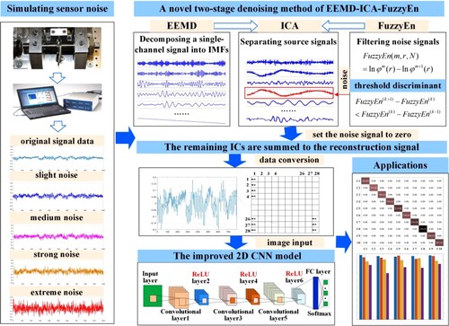
This paper develops a novel vibration signal denoising framework for condition monitoring and fault diagnosis in manufacturing processing. In this architecture, EEMD first decomposes the given signal into several IMFs as the input sources of ICA. Then, the decomposed IMFs can be separated into uncorrelated ICs. By calculating the FuzzyEn value of ICs as the threshold criterion, it can identify the noise components from all ICs and remove them. In this framework, the denoising task can be accomplished by reconstituting the denoised ICs and obtaining the reconstructed signal. Moreover, this paper proposes an improved CNN model with good noise immunity based on the VGG structure for practical manufacturing environments. The superior denoising and diagnosis performance of the proposed method have been verified on a rolling bearing dataset under various noise levels. The main contributions of the paper are as follows:

1. A new framework for machine fault diagnosis using the EEMD-ICA-FuzzyEn and CNN is proposed, which solves the problem of various noise interferences of machines. As a novel two-stage denoising method, it decomposes a single-channel signal into multiple components as different spectral modes by EEMD, satisfying the assumptions of ICA.

2. The produced independent components reconstruct the vibration signal data with the FuzzyEn value as the threshold criterion. The denoised signal is close to the original signal, following the principle of maximum correlation and minimum error.

3. The improved CNN model developed in this paper has outstanding noise immunity. The proposed network is based on VGG architecture with several convolution layers and activation layers, adding a batch normalisation layer to enhance model robustness. It can extract more information from the signals and achieve accurate diagnosis under the variable noise disturbance.

The remainder of this paper is organised as follows: Section 2 describes the related background. Section 3 presents the proposed method and its implementation. The experimental study, results, and discussion are presented in Section 4. Section 5 gives the conclusions and prospects for future work.

2. Related background

2.1. EEMD

EEMD is an improved method to alleviate the mode mixing problem occurring in EMD by adding finite white noise to the original signal data. The principle of the EEMD algorithm is as follows (Colominas, Schlotthauer, and Torres 2014). Firstly, ad a white noise series with the given amplitude to the original signal: (1) $x_m\left(t\right)=x\left(t\right)+w_m\left(t\right)$(1) in which $w_m\left(t\right)$ represents the mth trial added white noise series, $x\left(t\right)$ is the original signal series, and $x_m\left(t\right)$ means the noise-added signal. Then, using the EMD method, $x_m\left(t\right)$ would be decomposed into several IMFs and obtain the mode $c_{i,m}(i=1,2,\dots I)$. I is the number of IMFs and $c_{i,m}$indicates the ith IMF of the mth trial. This process should be repeated with different white noise series until $m\ge M$which M is the amplitude of the added white noise. Finally, the ensemble mean of the mth trial for each IMF can be calculated: (2) ${\overline{c}}_m=\frac{1}{M}{\sum }_{m=1}^M{c}_{i,m},i=1,2,\dots ,I,m=1,2,\dots ,M$(2) Where the mean ${\overline{c}}_m$ denotes the final IMFs.

2.2. ICA

The independent component analysis (ICA) algorithm is introduced to separate the residual noise and retain the source signal from IMFs, to maximise the retention of the effective information carried by the vibration signal. The theoretical foundation of ICA is described as follows. Firstly, denoting the random observed vector $\mathit{X}=[X_1,X_2,\dots ,X_m{]}^T$ whose $m$ elements are mixtures of $n$ independent elements of a random sources vector $\mathit{S}=[S_1,S_2,\dots ,S_n{]}^T$: (3) $\mathit{X}=\mathit{A}\mathbf{\ast }\mathit{S}$(3) where $\mathit{A}$ represents an unknown $m\times n$mixing matrix. The goal of ICA is to estimate the demixing matrix $\mathit{W}$ so that the reconstructed data matrix $\mathit{Y}$ can be given: (4) $\mathit{Y}\mathbf{=}\mathit{W}\mathit{X}\cong \mathit{S}$(4) where the unmixing matrix $\mathit{W}$is the inverse of $\mathit{A}$, and $\mathit{Y}$ is the best possible approximation of $\mathit{S}$. Based on the non-Gaussianity perspective, the FastICA algorithm presents a computationally efficient, fast, and popular ICA package.

2.3. Fuzzy Entropy (FuzzyEn)

Fuzzy Entropy can be used as the discriminant threshold to identify the noise components from all independent components (ICs) and set them to zero. The FuzzyEn algorithm can be described as follows. For the time series $\left\{u\left(i\right):1\le i\le N\right\}$, form vectors: (5) $\left\{{\mathit{X}}_i^m=\left\{u\left(i\right),u(i+1),\dots ,u(i+m-1)\right\}-u0\left(i\right)\right\}$(5) in which $i=1,\dots ,N-m+1$, and m means the amounts of u values. Then, we can calculate the similarity degree $D_{ij}^m$of its neighbouring vector ${\mathit{X}}_j^m$ by a fuzzy function: (6) $D_{ij}^m=\mu \left(d_{ij}^m,r\right)$(6) where $d_{ij}^m$ is the maximum absolute difference between the corresponding vectors of ${\mathit{X}}_i^m$ and ${\mathit{X}}_j^m$. For each vector ${\mathit{X}}_i^m$, we can define the FuzzyEn: (7) $\begin{array}{rl}& FuzzyEn(m,r,N)\\ & =\ln {\phi }^m\left(r\right)-\ln {\phi }^{m+1}\left(r\right)\\ & =\ln (N-m{)}^{-1}{\sum }_{i=1}^{N-m}{\varphi }_i^m\left(r\right)\\ & -\ln (N-m{)}^{-1}{\sum }_{i=1}^{N-m}{\varphi }_i^{m+1}\left(r\right)\end{array}$(7) where ${\varphi }_i^m\left(r\right)$ is the ${\mathit{X}}_i^m$ averaging the similarity degrees of all neighbouring vectors, getting ${\phi }^m\left(r\right)=(N-m{)}^{-1}{\sum }_{i=1}^{N-m}{\varphi }_i^m\left(r\right)$. After calculating the fuzzy entropy value of multi-components, a threshold discriminant method can identify source signals and noise signals (Gómez-Herrero et al. 2006), as shown below. (8) $FuzzyE{n}^{(k+1)}-FuzzyE{n}^{\left(k\right)}<FuzzyE{n}^{\left(k\right)}-FuzzyE{n}^{(k-1)}$(8) where $FuzzyE{n}^{\left(k\right)}$ represents the entropy of the kth independent component sorted in ascending order value. And k is the smallest integer in the range ⌊N/2⌋≥k > 1, the corresponding ICs are the noise signal and would be filtered by setting zero. The remaining ICs are summed to the reconstruction signal.

2.4. CNN

As a supervised deep learning method, CNN consists of convolutional layers, pooling layers, and full-connected layers, with three traits of the local field, subsampling, and weight sharing. As the key operation of CNN, the process of the convolutional layer is shown in Figure 1.

Figure 1. A calculation from the input to the output in the convolutional layer.

An computing example of the convolutional layer, the input feature mapping X is convolved with the convolution kernel. It can obtain the net input Z by adding a bias b in the convolution results. After a nonlinear activation function, the output feature mapping Y is obtained.

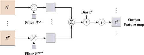
And the convolution kernel ${\mathit{W}}^p$ convolutes the input feature map ${\mathit{X}}^D$and adds it, with the function of the scalar bias b, obtaining the net input of the convolution layer ${\mathit{Z}}^p$. On this basis, the output feature map ${\mathit{Y}}^p$ is obtained through the activation function. (9) ${\mathit{Y}}^p=f\left({\mathit{Z}}^p\right)={\mathit{W}}^p\otimes \mathit{X}+b^p=\sum _{d=1}^D{\mathit{W}}^{p,d}\otimes {\mathit{X}}^d+b^p$(9) in which $f(\bullet )$ is a nonlinear activation function, such as the ReLU function.

3. The Proposed Method

In this paper, a novel two-stage denoising method, named EEMD-ICA-FuzzyEn, has been proposed. It decomposes a single-channel signal into multiple IMFs by EEMD. Then, ICA can separate the IMFs into several independent ICs. FuzzyEn discriminant value is the threshold to filter noise components from the ICs. By setting the noisy ICs to zero, the denoised ICs could be reconstructed into new signals_. Finally, the reconstruction signal is used as the input signal of the improved CNN model, which is adaptive for condition monitoring and fault diagnosis task under variable noisy environments. The flowchart of the developed method is shown in Figure 2. The detailed steps of the method are described as follows.

• Step 1. Collect vibration data from the monitored machine. To simulate real manufacturing processes, different levels of Gaussian noise are added to the collected vibration signal data. Under extreme noise environments, the validity of the proposed denoising approach and diagnosis model can be tested.

• Step 2. Decompose a single-channel signal into multiple IMFs. The EEMD method can decompose the vibration signal data into several IMFs and a residual component. IMFs can be as multi-dimensional source signals to satisfy the assumptions of ICA.

• Step 3. Separate source signals and filter noise components. ICA can separate the source signal from IMFs and obtain several uncorrelated ICs. By calculating the FuzzyEn value of ICs, it is a threshold criterion to identify the noise components from ICs and filter them. As result, the remaining ICs could be reconstructed into a new signal.

• Step 4. Construct the improved CNN model based on a VGG-like structure. The proposed CNN model based on the VGG architecture includes several convolution layers and activation layers and uses batch normalisation to enhance model robustness. It can achieve an accurate diagnosis and is resistant to noise interference, even extreme noise disturbance.

• Step 5. Construct the dataset and train the improved CNN model. In the data conversion process, the overlap sliding segmentation method is employed to scan the signal and generate the samples as the input data for CNN. After training, the proposed approach can provide excellent and robust diagnostic accuracy under variable noise disturbance. If a fault is observed, further analysis and maintenance strategies of the manufacturing equipment will be triggered.

Figure 2. The overall framework of the proposed method.

The flowchart of this paper: firstly, simulating the different sensor noise levels, including slight noise, medium noise, strong noise, and extreme noise; secondly, the original signal and noisy signals will be denoised by a novel two-stage denoising method, named EEMD-ICA-FuzzyEn; finally, the denoised signals will be as the input data into the improved CNN model for intelligent fault diagnosis.

4. Experimental validation

4.1. Fault data description of the rolling bearing

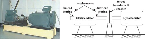
The roller bearing is the key component of many manufacturing equipments and its condition is critical to the production system. In this case study, the vibration signal of roller bearing from Case Western Reserve University (Case Western Reserve University Bearing Data Centre 2021) is utilised. The experiment setup is shown in Figure 3. The vibration signals of the drive-end bearing were collected under a 1 hp load scenario at a sampling frequency of 12 kHz. To cover the bearing fault types that can be encountered in the real application, three fault types, including inner race fault (IRF), ball fault (BF), and outer race fault (ORF) are considered. For each fault type, it has three fault levels, representing slight, moderate, and severe faults respectively. Thus, 10 rolling bearing operation conditions in total are considered in the experiment.

Figure 3. Test rig of rolling-element bearing.

Photograph of test rig of rolling-element bearing, it sequentially includes the electric motor, torque transducer & encoder, and dynamometer. And the accelerometers are installed on both the fan-end and the drive-end of the electric motor, which can measure the acceleration data of the test bearings.

Detailed sample distributions of the ten states of the rolling bearing are listed in Table 1. To reduce model training uncertainty, this paper expands the number of training and testing datasets during the sampling process by using the overlap sliding segmentation method, in which each segmentation signal is 784 sample points and the length of sample overlap for two neighbour segments is 684 sample points (Han et al. 2022). After the segmentation, for each bearing condition, 1000 samples with 100684 data points have been collected. In total, there are 10000 samples for the ten conditions. Then, the training, validation, and testing dataset are formed by randomly selecting 50%, 30%, and 20%. The performance of the fault diagnosis is quantified using the following four standard measures: accuracy, precision, recall, and F1 score which are widely used in the literature (Chen, Zhang, and Gao 2021): (10) $\begin{array}{rl}Accuracy& =\frac{TP+TN}{TP+FP+FN+TN}\end{array}$(10) (11) $\begin{array}{rl}Precision& =\frac{TP}{TP+FP}\end{array}$(11) (12) $\begin{array}{rl}Recall& =\frac{TP}{TP+FN}\end{array}$(12) (13) $\begin{array}{rl}F1& =\frac{2\times Precision\times Recall}{Precision+Recall}\end{array}$(13) where TP, FP, FN, and TN represent the number of true positive, false positive, false negative, and true negative outcomes, respectively.

Table 1. The structure of the data sets.

Fault Diameter (in)	Fault Types	Number of training/ validation/testing samples	Class Label
0	normal bearing(NB)	500/300/200	C1
0.007” (slight fault)	inner race fault (IRF)	500/300/200	C2
	ball fault (BF)	500/300/200	C3
	outer race fault (ORF)	500/300/200	C4
0.014” (moderate fault)	inner race fault (IRF)	500/300/200	C5
	ball fault (BF)	500/300/200	C6
	outer race fault (ORF)	500/300/200	C7
0.021” (severe fault)	inner race fault (IRF)	500/300/200	C8
	ball fault (BF)	500/300/200	C9
	outer race fault (ORF)	500/300/200	C10

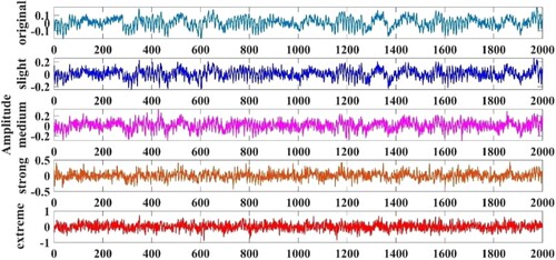
To simulate real working conditions with small disturbances in engineering, such as environmental noise, the Gaussian noise of various signal-to-noise ratios (SNR) is added to the testing data samples (Han, Li, and Qian 2021). The definition of SNR is shown as follows: (14) $SN{R}_{dB}=10{\log }_{10}\left(\frac{P_{signal}}{P_{noise}}\right)$(14) where $P_{signal}$ and $P_{noise}$ are the power of the original signal and the noisy signal, respectively. From the formula, when the SNR is 0 dB, it means the power of noise is equal to that of the original signal. Based on the literature, the range of noisy signals is usually from −10 dB to 10 dB, in which −10 dB belongs to extensive noise interference (Zhang et al. 2018; Jin et al. 2020). To evaluate the anti-interference capability of the proposed method, the SNR is set to 4, 0 dB, −4 dB, and −10 dB for slight, medium, strong, and extreme noise conditions, respectively. Vibration signals with Gaussian noise of different noise levels are plotted in Figure 4.

Figure 4. Different levels of Gaussian noise disturbance in normal bearing.

The amplitude of the original signal and four different noisy signals, increasing vibration amplitude as noise disturbance increases.

4.2. Two-stage joint denoising and reconstructing process

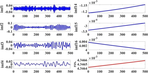
At the first stage of joint denoising, the single-channel signal is decomposed by EEMD with the ensemble number 50, and the added noise amplitude is set as 0.2 times the investigated signal standard deviation. The decomposition result is shown in Figure 5, including 16 IMF components and a reside. The IMF1, IMF2, and IMF3 components of the EEMD decomposition are sinusoidal intermittent signals containing high frequencies. Relatively, the IMF14, IMF15, and IMF16 components are well extracted from the low frequencies components of the signal. They belong to the multi-channel signal that meets the input requirements of the ICA algorithm.

Figure 5. The decomposition results using EEMD of normal bearing.

The decomposed several intrinsic mode functions components by using the method of ensemble empirical mode decomposition (EEMD), containing high frequencies, low frequencies, and a residence of the signal.

In the second stage, 15 independent components are produced from the multi-channel IMFs by using the FastICA algorithm with nonlinearity cubic power functions, shown in Figure 6. Normally, the number of ICs is less than that of IMFs (Cao and Lin 2017). Sorting the independent components in ascending order according to the fuzzy entropy value, can identify noise signals and set them to zero once not satisfied with Equation 8(8) $FuzzyE{n}^{(k+1)}-FuzzyE{n}^{\left(k\right)}<FuzzyE{n}^{\left(k\right)}-FuzzyE{n}^{(k-1)}$(8) . 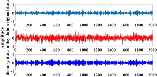In the example of the normal condition, the smallest fuzzy entropy value in order is IC3 (3.1861*10⁻⁵), IC5 (1.2524*10⁻⁴), and IC2 (1.7968*10⁻⁴), then IC3 and IC5 will be filtered as the noise signals referring the Equation 8(8) $FuzzyE{n}^{(k+1)}-FuzzyE{n}^{\left(k\right)}<FuzzyE{n}^{\left(k\right)}-FuzzyE{n}^{(k-1)}$(8) , as the red line of ICs shown in Figure 6. Then, the noise signals would be set to zero, and the remaining ICs are summed to produce the reconstructed vibration signal. Figure 7 presents the original signal, the strong noisy signal, and the denoised signal. It visually shows that the significant denoising effect as the denoised signal is similar to the original signal.

Figure 6. The separation results using Fast ICA-FuzzyEn under normal condition.

The independent components are separated from the multi-channel intrinsic mode functions by using the FastICA algorithm. And two independent components presented with the red line are filtered as the noise signals with fuzzy entropy values as the threshold criterion.

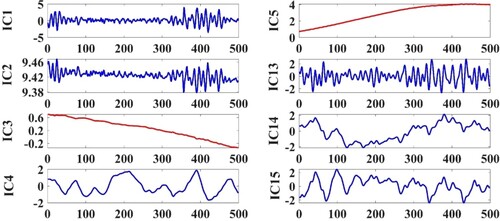
Figure 7. The original, noisy, and denoised signal of C3.

Choosing the rolling slight fault as an example, it presents the difference of amplitude among the original signal, added noise signal, and denoised signal.

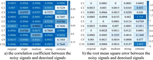
To further evaluate the effect of denoising, the correlation coefficient (CC) and root mean square error (RMSE) are calculated between the noisy signals and denoised signals (Jin, Li, and Mohamed 2019), as shown in Figure 8. The average correlation coefficient between the noisy signals and denoised signals under different noise levels, including original data, slight noise, medium noise, strong noise, and extreme noise, are 0.9872, 0.9671, 0.9640, 0.9411, and 0.8487, and the corresponding RMSEs are 0.0007, 0.0025, 0.0135, 0.0099, and 0.4063, respectively. These represent that the denoised signal is close to the noisy signal, following the principle of maximum correlation and minimum error. In the extreme noise condition, more noise signal is removed, so the correlation coefficient between the corrupted and denoised signal decreases, and the corresponding RMSE becomes larger. The result shows that the proposed approach achieves better denoising effectiveness with higher levels of noise interference.

Figure 8. Evaluation denoising results among different noise levels.

The picture on the left is the correlation coefficient between the noisy signals and denoised signals under original data and different noise levels; the right graph is the root mean square error values between them. And the darker the colour, the larger the number.

4.3. Fault diagnosis result using the proposed method

In the experiments, Matlab 2020a is used as the software with the hardware of NVIDIA GeForce RTX 3050Ti. After the grid search of the hyperparameters, the optimum batch size is set as 128, and the network structure of the improved CNN model is determined, as shown in Table 2. To comply with the input requirements of the 2D CNN, each sample with 784 data points is first reshaped to the size of 28*28.

Table 2. Parameter settings of the EEMD-ICA-FuzzyEn and CNN model.

Method	Parameters	Value
EEMD	noise standard deviation (Nstd)	0.2
	number of realizations (Yang, Liu, and Zio)	50
	maximum number of sifting iterations allowed (MaxIter)	50
ICA	approach	Deflation
	nonlinearity approach	Power3
	stabilization	off
FuzzyEn	standard deviation (SD)	r = 0.2
	number of continuous variables	m = 2
	threshold discriminant	Satisfy
Improved CNN	convolution kernel 1	Weights 5*5*1*20; bias 1*1*20
	relu function 2	ReLU
	pooling layer 3	Maxpooling 2*2
	convolution kernel 4	Weights 5*5*20*40; bias 1*1*40
	relu function 5	ReLU
	convolution kernel 6	Weights 5*5*40*100; bias 1*1*100
	relu function1 7	ReLU
	batch_normalisation 8	Batch_normalisation
	full-connected layers 9	Weights 10*25600; bias 10*1
	softmax 10	Softmax

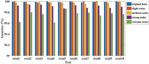
To test model robustness and reduce the impact of contingency on the diagnosis results, ten trials are run with original data and different denoised data. The detailed results of accuracy are shown in Figure 9. For each run, the overall classification performance is the average accuracy value of C1-C10. The testing accuracy for five denoised data by the proposed CNN reaches 99.99%, 99.99%, 99.97%, 99.91%, and 99.75%, meanwhile, the average precision values are 99.96%, 99.95%, 99.87%, 99.55%, and 98.75%, respectively. The result shows the proposed denoising and diagnosis approach can be applied to manufacturing equipment key components diagnosis, effectively preventing diagnostic degradation caused by noise.

Figure 9. The repeated diagnosis results in denoised data with different noise levels.

The accuracy results in ten trials, with original data and different denoised data as input data to the improved CNN, outperform with high accuracy and slight influence by noise interference.

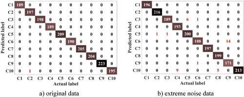
For the first trial, the testing accuracy of original data and extreme noise data is 99.99% and 99.62%, and the precision reaches 99.95% and 98.18%. The confusion matrix is shown in Figure 10. The highlighted diagonal values represent the correctly classified sample number of each state, and the other displaying red values represent the number of misclassified samples. The proposed denoising and diagnosis model achieves more than 99% accuracy even under extreme noise disturbance. In extreme noise environments, there are some slight misclassifies between C6 (moderate fault of the ball) and C9 (severe fault of the ball), as shown in Figure 10 b).

Figure 10. Confusion matrix with the original data and extreme noise as representatives.

The picture presents diagnosis performance for original data and extreme noise by the confusion matrix. And the highlighted diagonal values represent the correctly classified sample number of each state, and the other displaying red values belong to misclassified samples.

The effectiveness of the proposed two-stage joint denoising is discussed here through the comparison with the same classifier. The former of the results in the table is the performance of the denoising data and the latter belongs to the noisy data. With different levels of noise interference, the average values of the overall testing accuracy are 99.96%, 99.89%, 99.71%, 99.14%, and 96.91%, respectively. Using the proposed denoising method, the diagnostic accuracies are improved by 0.03% to 2.84%. More details of performance comparison are listed in Table 3. Under the extreme noise environment, there is a significant improvement in recall, precision, and F1 score, 14.19%, 12.88%, and 14.57% respectively. The results confirm the superior denoising performance of the proposed denoising framework for fault diagnosis of manufacturing equipment, especially for the nonstationary vibration data under noise interference.

Table 3. Fault diagnosis performance comparison of noisy data and denoising data.

Noise level	Accuracy (%)	Recall (%)	Precision (%)	F1 score (%)
original	99.99 / 99.96	99.96 / 99.79	99.96 / 99.79	99.96 / 99.79
slight	99.99 / 99.89	99.94 / 99.46	99.95 / 99.46	99.95 / 99.46
medium	99.97 / 99.71	99.86 / 98.53	99.87 / 98.53	99.86 / 98.52
strong	99.91 / 99.14	99.55 / 95.75	99.55 / 95.83	99.55 / 95.73
extreme	99.75 / 96.91	98.77 / 84.58	98.75 / 85.87	98.75 / 84.18

4.4. Comparisons with other methods

To prove the superior performance of the proposed denoising method, other conventional denoising methods are compared and the results are shown in Table 4. Denoising performance is tested under four noise levels, including SNR =  4, 0 dB, −4 dB, and −10 dB, to demonstrate the effectiveness and robustness of the proposed EEMD-FuEn-ICA denoising method. The proposed two-stage joint denoising method achieves nearly 100% accuracy on test samples under variable noise levels. Under the heavy noise environment, it remarkably outperforms the EMD-FuEn-ICA and EEMD with higher accuracy and robustness, which illustrates that the proposed denoising framework can be applied in complex noise scenarios in real applications.

Table 4. Comparison of diagnostic accuracy with other denoising methods.

Method	Original Data	Slight noise	Medium noise	Strong noise	Extreme noise
EEMD-FuEn-ICA	99.99	99.99	99.97	99.91	99.75
EMD-FuEn-ICA	99.99	99.95	99.82	99.72	99.08
EEMD	99.96	99.90	99.77	99.31	97.36

To further demonstrate the effectiveness of the denoising and diagnostic framework proposed in this paper, other state-of-the-art fault diagnosis methods are compared, with the results shown in Table 5. The improved CNN model with denoised data as input signal has better anti-interference capability than all other fault diagnosis models. Without denoising, the performance of the proposed method reaches more than 99% under slight, medium, and strong noise interference. With extreme noise, the LDR-CNN shows a slightly higher accuracy than the proposed model by 0.45%. Overall, compared to other DL methods, the proposed method provides robust denoising and intelligent diagnosis framework under variable noisy environments.

Table 5. Comparison of diagnostic accuracy with other DL approaches.

Method	Original Data	Slight noise	Medium noise	Strong noise	Extreme noise
The proposed method (denoised)	99.99	99.99	99.97	99.91	99.75
The proposed method (no denoising)	99.96	99.89	99.71	99.14	96.91
Ensemble TICNN (Zhang et al. 2018)	99.71	99.48	96.04	68.29	/
LDR-CNN (Ma et al. 2019)	100	99.82	99.45	98.88	97.36
Deep Transfer Learning(Li et al. 2019)	98.92	97.16	96.65	93.41	/
AAnNet(Jin et al. 2020)	99.83	99.66	99.83	98.97	59.31
MCNN-LSTM (Chen, Zhang, and Gao 2021)	98.46	88.19	81.41	77.27	/

5. Conclusions

In this paper, a CNN-based approach with a two-stage joint denoising method was proposed for intelligent fault diagnosis of rotating machinery. Effective signal denoising was achieved to increase the diagnosis accuracy and robustness. EEMD was used to decompose a single-channel signal into multiple independent components to satisfy the assumption of ICA, with the FuzzyEn as the threshold criterion to identify the noise signal. Experimental studies on roller bearings verified the diagnosis performance of the proposed approach. The denoised signal is close to the noisy signal with maximum correlation and minimum error. Moreover, accuracy can reach over 96.91% under different noisy conditions, especially in extreme noise environments. With effective denoising, the proposed 2D CNN model can achieve over 99.75% accuracy and 98.75% F1 score under variable noise environments. The comparison with the denoising methods and the state-of-the-art diagnosis methods showed that the proposed method can achieve more accurate and robust performance. Also, the remarkable anti-interference capability of the proposed diagnosis framework would enable its wide application in machinery fault diagnosis under strong noise environments.

The study has some limitations which could be addressed in future studies. First, the real-time performance of the developed model needs to be further validated for online monitoring. Second, more case studies of different machines can be carried out to evaluate the generalisation capability of the proposed framework. Third, varying working conditions of the production equipment should be considered to test the robustness of the method.

Acknowledgments

The authors are grateful for the comments by the reviewers and editors.

Data availability statement

The data that support the findings of this study are openly available on the Case Western Reserve University Bearing Data Centre Website at https://engineering.case.edu/bearingdatacenter/download-data-file.

Disclosure statement

No potential conflict of interest was reported by the author(s).

Additional information

Funding

This work was supported by Royal Society (grant number IES/R2/212028) and China Scholarship Council (CSC) (grant number 202106840063).

Notes on contributors

Hanting Zhou

Hanting Zhou is currently a Ph.D. student majoring in Management Science and Engineering at Nanjing University of Science and Technology, China. Meantime, she is a visiting Ph.D. student majoring in the School of Engineering at Lancaster University, UK. She received a B.S. degree (2016) and M.S. (2019) from China Jiliang University, China. Her research interests include smart manufacturing, signal processing, machine diagnosis and prognostics, and trustworthy AI.

Wenhe Chen

Wenhe Chen is currently pursuing the Ph.D. degree at the Nanjing University of Science and Technology, China. He received the B.S. degree from Eastern Liaoning University, China (2016); the M.S. degree from Anhui University of Technology, China (2020). His current research interests include data mining, deep neural networks, renewable energy equipment, fault diagnosis, optimisation algorithms.

Changqing Shen

Changqing Shen received the B.S. and Ph.D. degrees in Instrument Science and Technology from the University of Science and Technology of China in 2009 and 2014, respectively. He also obtained the Ph.D. degree in Systems Engineering and Engineering Management from the City University of Hong Kong in 2014. He is currently a Professor with the School of Rail Transportation, Soochow University, China. His research interests include machinery data mining, and intelligent fault diagnosis.

Longsheng Cheng

Longsheng Cheng is currently a professor of management sciences and applied statistics at the School of Economics and Management, Nanjing University of Science and Technology, China. He received his bachelor's degree from Anhui Normal University, China (1985), M.S. degree from East China Institute of Technology, China (1989), and Ph.D. degree from Nanjing University of Science and Technology, China (1998). His current research interests include prognostics and health management, machine learning, quality engineering, and applied statistics.

Min Xia

Min Xia is currently an Assistant Professor in the School of Engineering at Lancaster University, UK. He received B.S. degree in Industrial Engineering from Southeast University, China (2009); M.S. degree in Precision Machinery and Precision Instrumentation from the University of Science and Technology of China, China (2012); and Ph.D. degree in Mechanical Engineering from the University of British Columbia, Canada (2017). He has led 11 research projects in the UK, Canada, and Japan with total funding of £9 million. He has served various editorial roles including Associate Editor of IEEE Transactions on Instrumentation and Measurements. His research interests include smart manufacturing, machine diagnostics and prognostics, deep neural networks, process monitoring and optimisation.

References

- Alqahtani, Mejdal A, Myong K Jeong, and Elsayed A Elsayed. 2021. “Generalised Spatially Weighted Autocorrelation Approach for Monitoring and Diagnosing Faults in 3D Topographic Surfaces.” International Journal of Production Research. doi:10.1080/00207543.2021.2010825.
- Cao, Zehong, and Chin-Teng Lin. 2017. “Inherent Fuzzy Entropy for the Improvement of EEG Complexity Evaluation.” IEEE Transactions on Fuzzy Systems 26 (2): 1032–1035.
- “Case Western Reserve University Bearing Data Centre Website.” 2021. In., edited by https://engineering.case.edu/bearingdatacenter/download-data-file
- Chen, Mu-Chen, Chun-Chin Hsu, Bharat Malhotra, and Manoj Kumar Tiwari. 2016. “An Efficient ICA-DW-SVDD Fault Detection and Diagnosis Method for non-Gaussian Processes.” International Journal of Production Research 54 (17): 5208–5218.
- Chen, Xiaohan, Beike Zhang, and Dong Gao. 2021. “Bearing Fault Diagnosis Base on Multi-Scale CNN and LSTM Model.” Journal of Intelligent Manufacturing 32 (4): 971–987.
- Colominas, Marcelo A, Gastón Schlotthauer, and María E Torres. 2014. “Improved Complete Ensemble EMD: A Suitable Tool for Biomedical Signal Processing.” Biomedical Signal Processing and Control 14: 19–29.
- Fu, Qiang, Bo Jing, Pengju He, Shuhao Si, and Yun Wang. 2018. “Fault Feature Selection and Diagnosis of Rolling Bearings Based on EEMD and Optimized Elman_AdaBoost Algorithm.” IEEE Sensors Journal 18 (12): 5024–5034.
- Gómez-Herrero, Germán, Wim De Clercq, Haroon Anwar, Olga Kara, Karen Egiazarian, Sabine Van Huffel, and Wim Van Paesschen. 2006. Automatic removal of ocular artifacts in the EEG without an EOG reference channel. Paper presented at the Proceedings of the 7th Nordic signal processing symposium-NORSIG 2006.
- Han, Te, Yan-Fu Li, and Min Qian. 2021. “A Hybrid Generalization Network for Intelligent Fault Diagnosis of Rotating Machinery Under Unseen Working Conditions.” IEEE Transactions on Instrumentation Measurement 70: 1–11.
- Han, Haoran, Huan Wang, Zhiliang Liu, and Jiayi Wang. 2022. “Intelligent Vibration Signal Denoising Method Based on non-Local Fully Convolutional Neural Network for Rolling Bearings.” ISA Transactions 122: 13–23.
- Huo, Zhiqiang, Miguel Martínez-García, Yu Zhang, Ruqiang Yan, and Lei Shu. 2020. “Entropy Measures in Machine Fault Diagnosis: Insights and Applications.” IEEE Transactions on Instrumentation and Measurement 69 (6): 2607–2620.
- Jin, Tao, Qiangguang Li, and Mohamed A Mohamed. 2019. “A Novel Adaptive EEMD Method for Switchgear Partial Discharge Signal Denoising.” IEEE Access 7: 58139–58147.
- Jin, Guoqiang, Tianyi Zhu, Muhammad Waqar Akram, Yi Jin, and Changan Zhu. 2020. “An Adaptive Anti-Noise Neural Network for Bearing Fault Diagnosis Under Noise and Varying Load Conditions.” IEEE Access 8: 74793–74807.
- Li, Jimeng, Qingwen Yu, Xiangdong Wang, and Yungang Zhang. 2020. “An Enhanced Rolling Bearing Fault Detection Method Combining Sparse Code Shrinkage Denoising with Fast Spectral Correlation.” ISA Transactions 102: 335–346.
- Li, Xiang, Wei Zhang, Qian Ding, and Xu Li. 2019. “Diagnosing Rotating Machines with Weakly Supervised Data Using Deep Transfer Learning.” IEEE Transactions on Industrial Informatics 16 (3): 1688–1697.
- Ma, Shangjun, Wenkai Liu, Wei Cai, Zhaowei Shang, and Geng Liu. 2019. “Lightweight Deep Residual CNN for Fault Diagnosis of Rotating Machinery Based on Depthwise Separable Convolutions.” IEEE Access 7: 57023–57036.
- Ma, Baoze, and Tianqi Zhang. 2020. “Single-Channel Blind Source Separation for Vibration Signals Based on TVF-EMD and Improved SCA.” IET Signal Processing 14 (4): 259–268.
- Meng, Erhao, Shengzhi Huang, Qiang Huang, Wei Fang, Lianzhou Wu, and Lu Wang. 2019. “A Robust Method for non-Stationary Streamflow Prediction Based on Improved EMD-SVM Model.” Journal of Hydrology 568: 462–478.
- Miao, Feng, and Rongzhen Zhao. 2020. “A new Fault Diagnosis Method for Rotating Machinery Based on SCA-FastICA.” Mathematical Problems in Engineering 2020: 1–12.
- Panzer, Marcel, and Benedict Bender. 2021. “Deep Reinforcement Learning in Production Systems: A Systematic Literature Review.” International Journal of Production Research 60 (13): 4316–4341.
- Plaza, E García, and PJ Núñez López. 2018. “Application of the Wavelet Packet Transform to Vibration Signals for Surface Roughness Monitoring in CNC Turning Operations.” Mechanical Systems and Signal Processing 98: 902–919.
- Rai, Rahul, Manoj Kumar Tiwari, Dmitry Ivanov, and Alexandre Dolgui. 2021. “Machine Learning in Manufacturing and Industry 4.0 Applications.” International Journal of Production Research 59 (16): 4773–4778.
- Sahu, Chandan K, Crystal Young, and Rahul Rai. 2021. “Artificial Intelligence (AI) in Augmented Reality (AR)-Assisted Manufacturing Applications: A Review.” International Journal of Production Research 59 (16): 4903–4959.
- Sharma, Ajit, Zhibo Zhang, and Rahul Rai. 2021. “The Interpretive Model of Manufacturing: A Theoretical Framework and Research Agenda for Machine Learning in Manufacturing.” International Journal of Production Research 59 (16): 4960–4994.
- Wang, Jun, Guifu Du, Zhongkui Zhu, Changqing Shen, and Qingbo He. 2020. “Fault Diagnosis of Rotating Machines Based on the EMD Manifold.” Mechanical Systems and Signal Processing 135: 106443.
- Wang, Zheng, Qingxiu Liu, Hansi Chen, and Xuening Chu. 2021. “A Deformable CNN-DLSTM Based Transfer Learning Method for Fault Diagnosis of Rolling Bearing Under Multiple Working Conditions.” International Journal of Production Research 59 (16): 4811–4825.
- Wang, Huan, Zhiliang Liu, Dandan Peng, and Yong Qin. 2019. “Understanding and Learning Discriminant Features Based on Multiattention 1DCNN for Wheelset Bearing Fault Diagnosis.” IEEE Transactions on Industrial Informatics 16 (9): 5735–5745.
- Wei, Yu, Yuantao Yang, Minqiang Xu, and Wenhu Huang. 2021. “Intelligent Fault Diagnosis of Planetary Gearbox Based on Refined Composite Hierarchical Fuzzy Entropy and Random Forest.” ISA Transactions 109: 340–351.
- Wen, Long, Xinyu Li, Liang Gao, and Yuyan Zhang. 2017. “A new Convolutional Neural Network-Based Data-Driven Fault Diagnosis Method.” IEEE Transactions on Industrial Electronics 65 (7): 5990–5998.
- Xia, Min, Teng Li, Lin Xu, Lizhi Liu, and Clarence W De Silva. 2017. “Fault Diagnosis for Rotating Machinery Using Multiple Sensors and Convolutional Neural Networks.” IEEE/ASME Transactions on Mechatronics 23 (1): 101–110.
- Xia, Min, Haidong Shao, Darren Williams, Siliang Lu, Lei Shu, and Clarence W de Silva. 2021. “Intelligent Fault Diagnosis of Machinery Using Digital Twin-Assisted Deep Transfer Learning.” Reliability Engineering & System Safety 215:107938.
- Yang, Boyuan, Ruonan Liu, and Enrico Zio. 2019. “Remaining Useful Life Prediction Based on a Double-Convolutional Neural Network Architecture.” IEEE Transactions on Industrial Electronics 66 (12): 9521–9530.
- Zhang, Wei, Chuanhao Li, Gaoliang Peng, Yuanhang Chen, and Zhujun Zhang. 2018. “A Deep Convolutional Neural Network with new Training Methods for Bearing Fault Diagnosis Under Noisy Environment and Different Working Load.” Mechanical Systems and Signal Processing 100:439–453.
- Zhang, Chengyi, Jianbo Yu, and Shijin Wang. 2021. “Fault Detection and Recognition of Multivariate Process Based on Feature Learning of one-Dimensional Convolutional Neural Network and Stacked Denoised Autoencoder.” International Journal of Production Research 59 (8): 2426–2449.