A multi-start route improving matheuristic for the production routeing problem

Abstract

This paper considers the multi-vehicle production routeing problem with a maximum-level replenishment policy. This is a well-established problem within vendor managed inventory where production, inventory and routeing decisions are made simultaneously. We present a novel method to solve the problem that outperforms existing methods both in terms of solution gaps and the number of best-known solutions. The proposed matheuristic is tested on three different sets of benchmark instances consisting of 1218 instances and finds or improves the best-known solution for 632 of them. For the remaining instances, the matheuristic is less than 2.5% from the best-known solutions. The method is particularly proficient on large instances and is also efficient for the inventory routeing problem. The success of the method is largely due to its improvement phase where a novel path-flow-inspired mathematical model is introduced. Here, a route set obtained from the current solution is used and retailers can be simultaneously inserted and removed from a route, making the method flexible even when a small route set is used. In addition, we introduce a new production subproblem that approximates the costs of using a vehicle instead of approximating the costs of visiting a retailer, making it very fast to solve.

Keywords:

• Transportation
• production routeing
• matheuristic
• inventory routeing
• heuristic

1. Introduction

Effective supply chains are becoming increasingly important in a global and competitive world, and integrating the supply chain management is one of the most important measures to reduce supply chain costs and increase efficiency (Kumar et al. 2020). Traditionally, each stage of a supply chain, such as production, transportation, and inventory management, have been treated as separate problems, often handled sequentially by different decision-makers (Adulyasak, Cordeau, and Jans 2014a). However, recently it has become less common to treat these stages individually (Chen et al. 2021), as research has shown that there is a significant potential for savings by combining decisions from several stages into one planning problem (Archetti and Speranza 2016; Hrabec, Hvattum, and Hoff 2022). One such supply chain planning problem, which includes all three stages listed above, is the production routeing problem (PRP).

The PRP is a well-studied problem that has received increasing interest in the last two decades (Adulyasak, Cordeau, and Jans 2015). In its standard version, as it is presented in the routeing and lot-sizing literature, it consists of a single plant that produces a product which it distributes to multiple retailers over a finite multi-period time horizon with a fleet of identical vehicles with limited capacity. The retailers keep an inventory of the product and consume a specified number of units in each time period. Each retailer, as well as the plant, has limited storage capacity and no stock-outs are allowed. The decisions made for each time period is whether to start production or not and, if so, how much to produce, how much to deliver to each retailer, and for each vehicle decide which retailers it should visit, and in what sequence. The objective is to find the set of decisions that minimise the total setup, production, inventory holding, and transportation costs.

The PRP is a generalisation of the well-known inventory routeing problem (IRP) from the routeing literature because the IRP is a PRP where the production quantities are assumed to be known or unlimited. Both the PRP and the IRP fall under the business practice called vendor managed inventory (VMI). This is a policy where the supplier monitors the retailers' inventory and decides on the replenishment policy for each retailer. As a result, the supplier can coordinate shipments better and reduce its routeing costs, while the retailer can save time and effort on inventory management since they know that the supplier will ensure that they always have enough products in stock. Different industries are now implementing or exploring VMI systems, and practical examples include distribution of liquid air products, refilling vending machines, assembly of electronics, distribution of goods to chain stores, among others (Andersson et al. 2010; Coelho, Cordeau, and Laporte 2014). Recent reviews by Ma, Pal, and Gustafsson (2019) and Duong and Chong (2020) also highlight the importance, and potential benefits, of VMI and other variants of supply chain collaboration.

The PRP can be seen as a combination of the capacitated lot-sizing problem (Karimi, Fatemi Ghomi, and Wilson 2003) and the capacitated vehicle routeing problem (CVRP) (Laporte 2009). Hence, it is challenging to solve the PRP as it combines two NP-hard problems. Several methods have been proposed to solve the problem. Nevertheless, we believe that there is still room for improvement, especially for larger instances. The purpose of this paper is thus to improve the current state of the art and develop a better solution method that lets both industry and academia find better solutions to larger instances of the PRP.

1.1. Literature review

Most research on the PRP and its variants, including this work, considers a finite time horizon with discrete planning periods and the proposed models are typically formulated as mixed integer linear programs. The first researchers to address a variant of the PRP was Chandra (1993) who studied a multi-product production problem with an uncapacitated order size and an unlimited fleet of capacitated vehicles. This work was extended by Chandra and Fisher (1994) to include production setup costs, and the authors gave a formal definition of the problem. Over the years, numerous researchers have studied different versions of this problem where some have added features such as heterogeneous fleets (Low et al. 2014; Lei et al. 2006), multiple plants (Li et al. 2020; Juman et al. 2021), multiple products (Brahimi and Aouam 2016), perishable products (Farghadani-Chaharsooghi et al. 2022; Ghasemkhani et al. 2022), and tardiness costs (Long, Pardalos, and Li 2022). However, the majority of the research considers a single production plant with a constrained production capacity where the plant produces a single product for multiple retailers. Also, there are both inventory costs and inventory capacities at the retailers and the plant (Bard and Nananukul 2009; Archetti et al. 2011; Adulyasak, Cordeau, and Jans 2014a, 2014b; Absi et al. 2015; Solyalı and Süral 2017; Manousakis et al. 2022). This version of the problem has become known as the standard PRP and is the focus of this work. We refer to the survey by Adulyasak, Cordeau, and Jans (2015) for more information on the PRP, its applications, and different versions.

There are two main ways to classify both the standard PRP and the standard IRP. The first relates to the number of vehicles available, where we distinguish between problems with a single vehicle and those with multiple vehicles. Traditionally, the single-vehicle versions have mostly been solved by exact methods. However, with the advancement of computer technology, the multi-vehicle versions are now the most commonly studied. The second classification concerns replenishment policies for the retailers and two main policies have been considered in the inventory and production routeing literature (Archetti et al. 2007). The first is called order-up-to-level (OU) policy and states that every time a retailer is visited the delivered quantity is such that the inventory level reaches its maximum. The second, called maximum-level (ML) policy, allows the delivery of any quantity to a retailer as long as it does not exceed the maximum inventory level. In addition, a third policy exists where there are no constraints on the shipping quantity. This is referred to as replenishment policy (RP) by Zhang et al. (2021). The OU policy has mostly been addressed by exact methods, while heuristics have almost solely focussed on the less strict ML policy.

Due to the above-mentioned complexity, there are only a few exact algorithms for the PRP. The majority has used a branch-and-cut algorithm to solve the problem. This includes Ruokokoski et al. (2010) who studied the single-vehicle PRP with RP policy, Archetti et al. (2011) who compared the ML and OU policy for the single-vehicle PRP and Adulyasak, Cordeau, and Jans (2014a) and Schenekemberg et al. (2021) who solved multi-vehicle versions of the IRP and PRP with both OU and ML policies. In addition, Zhang et al. (2021) used a Benders' decomposition approach for the multi-vehicle PRP with OU policy. However, exact methods are only able to solve relatively small instances of the problem to optimality and struggle with realistically sized instances. The largest instances that have been solved to optimality consist of 50 retailers, three time periods and four vehicles for both ML and OU policies (Schenekemberg et al. 2021; Zhang et al. 2021).

As a result, the complexity of the problem has motivated the study of heuristic solution methods for the PRP. Several heuristics have been developed and they include a memetic algorithm by Boudia and Prins (2009), tabu search heuristics by Bard and Nananukul (2009) and Armentano, Shiguemoto, and Løkketangen (2011), an adaptive large neighbourhood search heuristic by Adulyasak, Cordeau, and Jans (2014b) and a variable neighbourhood search heuristic by Qiu et al. (2018). However, the advancement of CPUs and mixed integer linear programming (MILP) solvers in the last few decades have led to the success of heuristics that integrate mathematical programming techniques into a heuristic framework. These heuristics are often referred to as matheuristics (Boschetti et al. 2009). The survey of Archetti and Speranza (2014) highlights the contributions of matheuristics to routeing problems and their success in solving problems that combine routeing with other activities, such as production and/or inventory control.

Most matheuristics created for the PRP decompose the problem into a production problem and a routeing problem. First, the production problem is solved to construct production and distribution schedules before the routeing problem creates vehicle routes based on these schedules. This decomposition is, for instance, used by Archetti et al. (2011) and Absi et al. (2015) who both iterate between the two problems. In each iteration, the routes from the previous iteration are used to approximate costs in the production problem, which is then re-solved before new routes are created based on the latest production and distribution schedules.

In Avci and Yildiz (2019), a multi-start matheuristic is presented, where the production problem is solved by randomly constructing a distribution schedule and an associated production schedule in each restart. New routes are then constructed based on the latest schedules. Manousakis et al. (2022) presented a two-phase method where the production problem is solved in the first phase. The routes are then constructed by a local search which explores both the feasible and infeasible solution space in the second phase. The method is currently the one with the best reported results for the PRP, and the authors were able to find 594 and 55 new best solutions out of 1440 and 90 well-established benchmark instances. Li et al. (2019) proposed a three-level method where the first level solves the production subproblem and the second level determines the routeing. The third level is a fix-and-optimise procedure to improve the solution.

Chitsaz, Cordeau, and Jans (2019) on the other hand, introduced a three-phase iterative matheuristic where the production subproblem is further split into two parts, one determining the production schedule and the second determining the distribution schedule, before the routeing decisions are made in the third subproblem. Solyalı and Süral (2017) introduced a five-phase method where the production subproblem is solved in the two first phases. Then, the routeing subproblem is solved in the third phase before infeasible solutions obtained in the third phase are repaired and improved in the fourth and fifth phases. The majority of the papers mentioned above solve either VRPs or TSPs to determine the routeing, while the production subproblem is solved as a MILP.

A method that uses a slightly different decomposition was introduced by Russell (2017). The paper presents two heuristics where routes are constructed before the production and distribution schedules are created. In the first, a set of routes are generated and used in an approximate route-based model to fix the production and distribution decisions before the routes are improved using tabu search. As a final step, a procedure similar to the one developed by Absi et al. (2015) is used to improve the solution further. The second heuristic extends the concept of seed points from Fisher and Jaikumar (1981) to seed routes. The seed routes are then used in a model where retailers are added to the seed routes to get deliveries. Similar to the first heuristic, this model fixes the production and distribution decisions before the routes are improved using tabu search.

Many solution methods have been proposed for the standard IRP. We briefly highlight the most recent solution methods and refer to the survey papers of Andersson et al. (2010) and Coelho, Cordeau, and Laporte (2014) for more details on the IRP and its solution methods. The solution methods that have the lowest reported average gaps on large benchmark instances for the IRP include the branch-and-cut algorithms of Coelho and Laporte (2013), Guimarães et al. (2020) and Manousakis et al. (2020). Further, the heuristics with the lowest reported gaps include Archetti et al. (2012) who developed a matheuristic that combines tabu search with the solution of MILPs and the above-mentioned three-phase decomposition matheuristic of Chitsaz, Cordeau, and Jans (2019). In addition, the matheuristics of Archetti et al. (2021) and Solyalı and Süral (2022) have reported good results. The former is a kernel search heuristic, and the latter solves three subsequent MILPs of a restricted version of the problem. The first two MILPs construct a feasible solution, before the third tries to improve it. Finally, the method with the lowest reported average gap and the highest number of best-known solutions (BKSs) is the matheuristic of Vadseth, Andersson, and Stålhane (2021). The method iterates between solving a path-flow model with a small set of routes and updating the route set based on the optimal solution from the previous iteration.

As seen in the literature reviewed above, most matheuristics for the PRP and several matheuristics for the IRP decompose the problem into one production/distribution subproblem and one routeing subproblem typically consisting of one VRP (or several TSPs) for each time period, though some heuristics decompose the problem further. The main advantage of this approach is that it enables the heuristics to use state-of-the-art algorithms for the VRP and TSP, respectively, and that the production/distribution problem is usually a MILP with few integer variables, that is thus relatively easy to solve. The disadvantage of this decomposition approach is that the heuristics cannot correctly evaluate how decisions made in one problem affects the decisions in the other, since changes to the route of one vehicle may affect both the vehicle routes in other time periods and the production and distribution schedules of the plant and retailers. Therefore these matheuristics either use pre-defined rules to adjust the vehicle routes, or try to approximate the cost of making certain changes to a route.

1.2. Our contributions

We have chosen to focus on the multi-vehicle PRP with ML policy, which is by far the most studied version of the standard PRP. To solve the problem, we have developed a novel matheuristic that first constructs a feasible starting solution which is subsequently enhanced by an improvement phase. A starting solution is constructed using the traditional decomposition, described above, where we split the problem into a production and a routeing subproblem. We formulate the production subproblem as a MILP. However, unlike Adulyasak, Cordeau, and Jans (2014b), Absi et al. (2015) and Manousakis et al. (2022), who estimate the costs of visiting a retailer in their production subproblem MILP, we introduce a new MILP model that estimates the cost of using a vehicle instead. This reduces the number of binary variables needed drastically and makes the model very fast to solve.

For the improvement phase, we introduce a completely new path-flow-inspired model to improve the solution. The main advantage of this model over what is done in earlier heuristics is that it includes both the vehicle routeing and the production and distribution decisions in the same problem. Thus, this avoids the shortcomings of the traditional decomposition. The model allows us to consider multiple changes to all the routes in the model simultaneously, while at the same time evaluating the effect of these changes on the production and distribution decisions. All these changes are evaluated exactly using the full objective function of the problem, rather than an approximate one. This leads to larger improvements in each iteration, and thus reduces the number of iterations needed to reach a high quality solution. In addition, when compared with a standard path-flow model with a reduced route set, the proposed method increases the changes we can make to a solution exponentially and allows us to reduce the size of the route set significantly. Finally, the process of constructing a solution and running the improvement phase is fast and lets us restart the process several times using different differentiation techniques to explore a larger part of the solution space.

The proposed method has proved to be very successful. For smaller benchmark instances with known optimal solutions, the matheuristic finds solutions close to optima. For the larger PRP benchmark instances introduced by Archetti et al. (2007) and Boudia, Louly, and Prins (2007), the proposed method outperforms the state of the art and finds or improves the best-known solution for 516 out of 960 benchmark instances and 75 out of 90 benchmark instances, respectively. In addition, the matheuristic has proved to be flexible, and can in contrast to most solution methods on the PRP successfully solve the IRP as well. For the set of large benchmark instances for the IRP released by Archetti et al. (2011), our proposed method finds, or improves, 73 out of 240 instances. This number is larger than for any other solution method in the literature. Further, it does so requiring less than 20$\mathrm{\%}$ of the computing time used by all other solution methods. In summary, this outperforms all solution methods from the literature and significantly improves the current state of the art.

The remainder of the paper is organised as follows. In Section 2, the standard PRP is defined and presented mathematically. The matheuristic is presented in detail in Section 3. The computational experiments are reported in Section 4, and concluding remarks are presented in Section 5.

2. Problem definition and mathematical model

The standard multi-vehicle production routeing problem with ML policy handles the repeated production and distribution of a single product from a plant to a set of retailers over a finite planning horizon. We formulate this problem on a graph $G(\mathcal{N},\mathcal{A})$ where $\mathcal{N}$ is a set of nodes $\mathcal{N}=\{0,1,\dots ,N\}$ consisting of N retailers and a plant denoted 0. We also introduce ${\mathcal{N}}^{\prime }=\{1,\dots ,N\}$ as the set of retailers. The set of arcs $\mathcal{A}\subset \mathcal{N}\times \mathcal{N}$ defines arcs between each pair of nodes. The problem is defined over a time horizon consisting of $\mathcal{T}=\{0,1,\dots ,T\}$ discrete time periods, where ${\mathcal{T}}^{\prime }=\{1,\dots ,T\}$ is the set of planning time periods. The parameter T is defined as the number of time periods in the planning horizon. We follow the established convention of using lowercase for variables and indices and uppercase for parameters.

In each time period $t\in {\mathcal{T}}^{\prime }$, V vehicles, each with a capacity Q, can be used to distribute the product. There is a cost $C_{\mathrm{ij}}$, associated with each arc $(i,j)\in \mathcal{A}$. Retailer i has a known demand, $D_{\mathrm{it}}$, in each time period t and a maximum, $U_i$, and minimum, $L_i$, inventory level. The plant can produce up to P units of the product at the beginning of each time period, at the expense of a setup cost, $C^S$, and a unit production cost $C^U$. Both the plant and the retailers have an inventory holding cost $C_i^H$ per unit of the product left in the inventory at the end of each time period. Each retailer can only be visited once per time period and has an inventory of $I_i$ at the beginning of the planning horizon. The problem consists of minimising the production, transportation, and inventory holding costs, while making sure that the inventory levels, both at the plant and the retailers, stay within their limits.

2.1. A path-flow formulation

The proposed path-flow formulation requires some additional notation. The set $\mathcal{R}$ contains all routes. A route is a Hamiltonian cycle through a subset of the nodes including the plant. Introducing $A_{\mathrm{ijr}}$ as 1 if route r traverses arc $(i,j)$, and 0 otherwise, the cost of route r can be defined as $C_r^T=\sum _{(i,j)\in \mathcal{A}}{C}_{\mathrm{ij}}{A}_{\mathrm{ijr}}$. The variable ${\lambda }_{\mathrm{rt}}$ is 1 if route r is used by a vehicle in time period t, and 0 otherwise. The quantity delivered at retailer i in time period t is denoted $q_{\mathrm{it}}$ and the inventory level at node i at the end of time period t is denoted $s_{\mathrm{it}}$. The variable $o_t$ is 1 if the plant produces in time period t, and 0 otherwise, while $p_t$ denotes the quantity produced in time period t. Finally, let $l_{\mathrm{ijt}}$ be the load on-board a vehicle driving from node i to node j in time period t. With this notation, a mathematical model of the production routeing problem can be formulated as follows:

(1) $\begin{array}{rl}\min \sum _{t\in {\mathcal{T}}^{\prime }}{C}^U{p}_t+\sum _{t\in {\mathcal{T}}^{\prime }}{C}^S{o}_t+\sum _{r\in \mathcal{R}}\sum _{t\in {\mathcal{T}}^{\prime }}{C}_r^T{\lambda }_{\mathrm{rt}}+\sum _{i\in \mathcal{N}}& \sum _{t\in {\mathcal{T}}^{\prime }}{C}_i^H{s}_{\mathrm{it}},\end{array}$(1) (2) $\begin{array}{rlrl}{p}_t& \le P{o}_t,& t\in {\mathcal{T}}^{\prime },& \end{array}$(2) (3) $\begin{array}{rlrl}{s}_{i0}& =I_i,& i\in \mathcal{N},& \end{array}$(3) (4) $\begin{array}{rlrl}{s}_{0t}-s_{0(t-1)}-p_t+\sum _{i\in {\mathcal{N}}^{\prime }}{q}_{\mathrm{it}}& =0,& t\in {\mathcal{T}}^{\prime },& \end{array}$(4) (5) $\begin{array}{rlrl}{s}_{\mathrm{it}}-s_{i(t-1)}+D_{\mathrm{it}}-q_{\mathrm{it}}& =0,& i\in {\mathcal{N}}^{\prime },t\in {\mathcal{T}}^{\prime },& \end{array}$(5) (6) $\begin{array}{rlrl}{L}_i\le s_{\mathrm{it}}& \le U_i,& i\in \mathcal{N},t\in \mathcal{T},& \end{array}$(6) (7) $\begin{array}{rlrl}\sum _{j\in \mathcal{N}}{l}_{\mathrm{jit}}-q_{\mathrm{it}}-\sum _{j\in \mathcal{N}}{l}_{\mathrm{ijt}}& =0,& i\in {\mathcal{N}}^{\prime },t\in {\mathcal{T}}^{\prime },& \end{array}$(7) (8) $\begin{array}{rlrl}{l}_{\mathrm{ijt}}& \le Q\sum _{r\in \mathcal{R}}{A}_{\mathrm{ijr}}{\lambda }_{\mathrm{rt}},& (i,j)\in \mathcal{A},t\in {\mathcal{T}}^{\prime },& \end{array}$(8) (9) $\begin{array}{rlrl}\sum _{r\in \mathcal{R}}\sum _{j\in \mathcal{N}}{A}_{\mathrm{ijr}}{\lambda }_{\mathrm{rt}}& \le 1,& i\in {\mathcal{N}}^{\prime },t\in {\mathcal{T}}^{\prime },& \end{array}$(9) (10) $\begin{array}{rlrl}\sum _{r\in \mathcal{R}}{\lambda }_{\mathrm{rt}}& \le V,& t\in {\mathcal{T}}^{\prime },& \end{array}$(10) (11) $\begin{array}{rlrl}{\lambda }_{\mathrm{rt}}& \in \{0,1\},& r\in \mathcal{R},t\in {\mathcal{T}}^{\prime },& \end{array}$(11) (12) $\begin{array}{rlrl}{o}_t& \in \{0,1\},& t\in {\mathcal{T}}^{\prime },& \end{array}$(12) (13) $\begin{array}{rlrl}{q}_{\mathrm{it}}& \ge 0,& i\in {\mathcal{N}}^{\prime },t\in {\mathcal{T}}^{\prime },& \end{array}$(13) (14) $\begin{array}{rlrl}{l}_{\mathrm{ijt}}& \ge 0,& (i,j)\in \mathcal{A},t\in {\mathcal{T}}^{\prime },& \end{array}$(14) (15) $\begin{array}{rlrl}{p}_t& \ge 0,& t\in {\mathcal{T}}^{\prime }.& \end{array}$(15)

The objective function (1(1) $\begin{array}{rl}\min \sum _{t\in {\mathcal{T}}^{\prime }}{C}^U{p}_t+\sum _{t\in {\mathcal{T}}^{\prime }}{C}^S{o}_t+\sum _{r\in \mathcal{R}}\sum _{t\in {\mathcal{T}}^{\prime }}{C}_r^T{\lambda }_{\mathrm{rt}}+\sum _{i\in \mathcal{N}}& \sum _{t\in {\mathcal{T}}^{\prime }}{C}_i^H{s}_{\mathrm{it}},\end{array}$(1) ) minimises the production, setup, transportation, and inventory holding costs over the entire planning horizon, while constraints (2(2) $\begin{array}{rlrl}{p}_t& \le P{o}_t,& t\in {\mathcal{T}}^{\prime },& \end{array}$(2) ) state that the plant can only produce if production is set up and the produced quantity must be within the production capacity. Constraints (3(3) $\begin{array}{rlrl}{s}_{i0}& =I_i,& i\in \mathcal{N},& \end{array}$(3) ) set the initial inventory level at each node. The inventory balance at the plant, which states that the inventory at the plant in a time period is equal to the sum of the inventory of the previous time period and the produced quantity with delivered quantity subtracted, is ensured by constraints (4(4) $\begin{array}{rlrl}{s}_{0t}-s_{0(t-1)}-p_t+\sum _{i\in {\mathcal{N}}^{\prime }}{q}_{\mathrm{it}}& =0,& t\in {\mathcal{T}}^{\prime },& \end{array}$(4) ). Similarly, the inventory balance of the retailers is stated by constraints (5(5) $\begin{array}{rlrl}{s}_{\mathrm{it}}-s_{i(t-1)}+D_{\mathrm{it}}-q_{\mathrm{it}}& =0,& i\in {\mathcal{N}}^{\prime },t\in {\mathcal{T}}^{\prime },& \end{array}$(5) ). Moreover, constraints (6(6) $\begin{array}{rlrl}{L}_i\le s_{\mathrm{it}}& \le U_i,& i\in \mathcal{N},t\in \mathcal{T},& \end{array}$(6) ) make sure that the inventory level at each node stays between its upper and lower limits. Constraints (7(7) $\begin{array}{rlrl}\sum _{j\in \mathcal{N}}{l}_{\mathrm{jit}}-q_{\mathrm{it}}-\sum _{j\in \mathcal{N}}{l}_{\mathrm{ijt}}& =0,& i\in {\mathcal{N}}^{\prime },t\in {\mathcal{T}}^{\prime },& \end{array}$(7) ) ensure that the difference in the load on-board a vehicle when arriving and leaving a retailer is equal to the quantity delivered. Constraints (8(8) $\begin{array}{rlrl}{l}_{\mathrm{ijt}}& \le Q\sum _{r\in \mathcal{R}}{A}_{\mathrm{ijr}}{\lambda }_{\mathrm{rt}},& (i,j)\in \mathcal{A},t\in {\mathcal{T}}^{\prime },& \end{array}$(8) ) force the load on-board a vehicle to not exceed the vehicle capacity, while constraints (9(9) $\begin{array}{rlrl}\sum _{r\in \mathcal{R}}\sum _{j\in \mathcal{N}}{A}_{\mathrm{ijr}}{\lambda }_{\mathrm{rt}}& \le 1,& i\in {\mathcal{N}}^{\prime },t\in {\mathcal{T}}^{\prime },& \end{array}$(9) ) state that a retailer cannot be visited more than once in a time period. With constraints (10(10) $\begin{array}{rlrl}\sum _{r\in \mathcal{R}}{\lambda }_{\mathrm{rt}}& \le V,& t\in {\mathcal{T}}^{\prime },& \end{array}$(10) ) we make sure that the maximum number of available vehicles is not exceeded. Finally, constraints (11(11) $\begin{array}{rlrl}{\lambda }_{\mathrm{rt}}& \in \{0,1\},& r\in \mathcal{R},t\in {\mathcal{T}}^{\prime },& \end{array}$(11) )–(15(15) $\begin{array}{rlrl}{p}_t& \ge 0,& t\in {\mathcal{T}}^{\prime }.& \end{array}$(15) ) define the variable domains.

We allow the sum of the inventory level in the previous time period and the delivered quantity $(s_{i(t-1)}+q_{\mathrm{it}})$ to exceed the maximum inventory capacity $U_i$ as long as the excessive quantity is consumed during time period t. In this way, the inventory $s_{\mathrm{it}}$ at the end of the period does not exceed the maximum inventory capacity. This is common practice in the PRP literature and allows us to compare our solutions with others. However, there are academic works that enforce a stricter policy forcing $q_{\mathrm{it}}+s_{i(t-1)}\le U_i,i\in {\mathcal{N}}^{\prime },t\in {\mathcal{T}}^{\prime }$ (Adulyasak, Cordeau, and Jans 2014a, 2015; Qiu et al. 2018).

3. Matheuristic

The formulation given in Section 2.1 is a complete formulation of the problem. However, since the set of routes $\mathcal{R}$ grows exponentially with the number of retailers, it is impossible to generate all routes within reasonable time for large instances of the problem. The main idea of the matheuristic proposed in this paper is to replace $\mathcal{R}$ with a smaller route set $\hat{\mathcal{R}}$, containing only a small set of ‘promising’ routes. However, finding these routes is not trivial and small changes to them can have a large impact on the objective value.

The proposed matheuristic is a multi-start route improving matheuristic, where each restart creates a new initial solution by first solving a production subproblem and then solving a routeing subproblem, similar to Archetti et al. (2011) and Absi et al. (2015). In each restart, the routes from the routeing subproblem are placed in the route set $\hat{\mathcal{R}}$, and the solution is improved for δ iterations by solving an improvement MILP that allows small changes to the routes in $\hat{\mathcal{R}}$. To ensure that we get a unique initial solution at each restart, a set of differentiation techniques, $\tilde{\mathcal{T}}$, is used to change the production subproblem. By diversifying the search, we make sure that we explore a larger part of the solution space and hence increase the chance of finding a good solution to the problem. Each differentiation technique $\tau \in \tilde{\mathcal{T}}$ is used ${ϵ}_{\tau }$ times and is based on the final solution of the previous iteration. In the last part of the matheuristic, we intensify the search around the best solution found during the multi-start phase of the heuristic by iteratively solving the improvement MILP with an extended route set. A pseudocode of the complete matheuristic is described in detail in Algorithm 1.

3.1. Generating a new initial solution

To obtain an initial solution to the multi-start heuristic, we first solve a production subproblem, which is a relaxation of the original PRP where the purpose is to make good production decisions. The model presented here is similar to the ones found in Adulyasak, Cordeau, and Jans (2014b), Absi et al. (2015) and Manousakis et al. (2022) where the routeing cost is approximated. However, unlike the mentioned papers, the routeing aspects of the problem are completely relaxed in this model, and no routeing decisions are considered in the production subproblem. Instead, we introduce an integer variable, $v_t$, deciding the number of vehicles used per time period. This is somewhat similar to the Benders' decomposition in Zhang et al. (2021) where the routeing decisions are made in the subproblem and additional variables determining the routeing costs are included in the master problem. Here, however, the cost of using a vehicle is set a priori and denoted $C^V$. This reduces the number of variables in the model significantly. In addition, a modified vehicle capacity, $Q^V$, is introduced. All other notation has the same meaning as in Section 2.1.

(16) $\begin{array}{rl}\min \sum _{i\in \mathcal{N}}\sum _{t\in {\mathcal{T}}^{\prime }}{C}_i^H{s}_{\mathrm{it}}+\sum _{t\in {\mathcal{T}}^{\prime }}{C}^V{v}_t+\sum _{t\in {\mathcal{T}}^{\prime }}{C}^S{o}_t& +\sum _{t\in {\mathcal{T}}^{\prime }}{C}^U{p}_t,\end{array}$(16) (17) $\begin{array}{rlrl}{p}_t& \le P{o}_t,& t\in {\mathcal{T}}^{\prime },& \end{array}$(17) (18) $\begin{array}{rlrl}{s}_{i0}& =I_i,& i\in \mathcal{N},& \end{array}$(18) (19) $\begin{array}{rlrl}{s}_{0t}-s_{0(t-1)}-p_t+\sum _{i\in {\mathcal{N}}^{\prime }}{q}_{\mathrm{it}}& =0,& t\in {\mathcal{T}}^{\prime },& \end{array}$(19) (20) $\begin{array}{rlrl}\sum _{i\in \mathcal{N}}{s}_{\mathrm{it}}-s_{i(t-1)}+D_{\mathrm{it}}-q_{\mathrm{it}}& =0,& i\in {\mathcal{N}}^{\prime },t\in {\mathcal{T}}^{\prime },& \end{array}$(20) (21) $\begin{array}{rlrl}\sum _{i\in {\mathcal{N}}^{\prime }}{q}_{\mathrm{it}}& \le Q^V{v}_t,& t\in {\mathcal{T}}^{\prime },& \end{array}$(21) (22) $\begin{array}{rlrl}{U}_i\ge s_{\mathrm{it}}& \ge L_i,& i\in \mathcal{N},t\in \mathcal{T},& \end{array}$(22) (23) $\begin{array}{rlrl}{Q}^V\ge q_{\mathrm{it}}& \ge 0,& i\in {\mathcal{N}}^{\prime },t\in {\mathcal{T}}^{\prime },& \end{array}$(23) (24) $\begin{array}{rlrl}{p}_t& \ge 0,& t\in {\mathcal{T}}^{\prime },& \end{array}$(24) (25) $\begin{array}{rlrl}{v}_t& \in \{0,1,\dots ,V\},& t\in {\mathcal{T}}^{\prime },& \end{array}$(25) (26) $\begin{array}{rlrl}{o}_t& \in \{0,1\},& t\in {\mathcal{T}}^{\prime }.& \end{array}$(26)

The objective function (16(16) $\begin{array}{rl}\min \sum _{i\in \mathcal{N}}\sum _{t\in {\mathcal{T}}^{\prime }}{C}_i^H{s}_{\mathrm{it}}+\sum _{t\in {\mathcal{T}}^{\prime }}{C}^V{v}_t+\sum _{t\in {\mathcal{T}}^{\prime }}{C}^S{o}_t& +\sum _{t\in {\mathcal{T}}^{\prime }}{C}^U{p}_t,\end{array}$(16) ) minimises the setup, production, vehicle, and inventory holding costs over the entire planning horizon. Constraints (17)–(20(20) $\begin{array}{rlrl}\sum _{i\in \mathcal{N}}{s}_{\mathrm{it}}-s_{i(t-1)}+D_{\mathrm{it}}-q_{\mathrm{it}}& =0,& i\in {\mathcal{N}}^{\prime },t\in {\mathcal{T}}^{\prime },& \end{array}$(20) ) are the same as constraints (2(2) $\begin{array}{rlrl}{p}_t& \le P{o}_t,& t\in {\mathcal{T}}^{\prime },& \end{array}$(2) )–(5(5) $\begin{array}{rlrl}{s}_{\mathrm{it}}-s_{i(t-1)}+D_{\mathrm{it}}-q_{\mathrm{it}}& =0,& i\in {\mathcal{N}}^{\prime },t\in {\mathcal{T}}^{\prime },& \end{array}$(5) ) in the original formulation and handle production and inventory. Constraints (21(21) $\begin{array}{rlrl}\sum _{i\in {\mathcal{N}}^{\prime }}{q}_{\mathrm{it}}& \le Q^V{v}_t,& t\in {\mathcal{T}}^{\prime },& \end{array}$(21) ) ensure that the total quantity delivered in a time period is less than the total capacity of the vehicles used. Constraints (22(22) $\begin{array}{rlrl}{U}_i\ge s_{\mathrm{it}}& \ge L_i,& i\in \mathcal{N},t\in \mathcal{T},& \end{array}$(22) )–(26(26) $\begin{array}{rlrl}{o}_t& \in \{0,1\},& t\in {\mathcal{T}}^{\prime }.& \end{array}$(26) ) define the variable domains.

As mentioned, the cost per vehicle, $C^V$, must be estimated a priori when we solve the production subproblem. In this paper we use the cost of the TSP solution, $C^{\mathrm{TSP}}$, of the graph $G(\mathcal{N},\mathcal{A})$ and define the cost per vehicle as (27) $C^V=\alpha C^{\mathrm{TSP}},$(27) where α is a parameter set a priori. The modified vehicle capacity, $Q^V$, is introduced to increase the possibility of finding a feasible solution in the routeing subproblem. The modified capacity is set lower than the actual capacity of the vehicles, and is calculated as (28) $Q^V=\text{β}Q,$(28) where β is a value between 0 and 1.

Given the solution to the production subproblem, the routeing subproblem consists of one CVRP for each time period $t\in {\mathcal{T}}^{\prime }$, where the quantity to deliver to each retailer i equals the variable values $q_{\mathrm{it}}^{\ast }$ from the optimal solution to the production subproblem. If $q_{\mathrm{it}}^{\ast }=0$, then retailer i is not visited in time period t. The VRP-heuristic used in this paper is the genetic algorithm presented in Vidal et al. (2012). We have used the open-source implementation which is described in Vidal (2020). The stopping criterion of the heuristic is set to 2,000 iterations without finding an improvement. If a feasible solution to the routeing subproblem is not found, the production subproblem is re-solved with $Q^V\leftarrow \text{β}{Q}^V$. This process is repeated until a feasible solution to the routeing subproblem is found.

3.2. Differentiation techniques

In Algorithm 1 we run a for-loop over the set $\tilde{\mathcal{T}}$ of differentiation techniques starting on line 3. The idea behind these techniques is inspired by the combinatorial Benders' cuts proposed in Codato and Fischetti (2006). The set consists of three techniques that make sure that no two restarts produce the same initial solution.

1. The first technique is to put no limitations on the production subproblem.

2. The second technique forces a change in the production plan. Define ${\mathcal{T}}^O=\{t\in {\mathcal{T}}^{\prime }|o_t^{\ast }=1\}$ as the set of time periods during which there is production in the previous solution. Adding the differentiation constraint (29) $\sum _{t\in {\mathcal{T}}^{\prime }\setminus {\mathcal{T}}^O}{o}_t+\sum _{t\in {\mathcal{T}}^O}(1-o_t)\ge 1$(29) to the production subproblem makes sure that the production decisions change. All previous differentiation constraints are added to the model in the initialisation process, preventing a repetition of solutions.

3. The third technique forces the solution of the production subproblem to use fewer time periods to distribute the product. The reasoning for having this technique is that the production subproblem often underestimates the costs of visiting different retailers and produces solutions where multiple time periods have a single vehicle leaving the plant. This is often not beneficial for the original problem. We introduce the variable $k_t$ which is 1 if any vehicles are used in time period t, and 0 otherwise, and add the following constraints to the initialisation model: (30) $\begin{array}{rlrl}{v}_t& \le V{k}_t,& t\in {\mathcal{T}}^{\prime },& \end{array}$(30) (31) $\begin{array}{rl}\sum _{t\in {\mathcal{T}}^{\prime }}{k}_t& \le \sum _{t\in {\mathcal{T}}^{\prime }}{k}_t^{\ast }-1,\end{array}$(31) (32) $\begin{array}{rlrl}{k}_t& \in \{0,1\},& t\in \mathcal{T}.& \end{array}$(32) Constraints (30(30) $\begin{array}{rlrl}{v}_t& \le V{k}_t,& t\in {\mathcal{T}}^{\prime },& \end{array}$(30) ) indicate if any vehicles are used and constraint (31(31) $\begin{array}{rl}\sum _{t\in {\mathcal{T}}^{\prime }}{k}_t& \le \sum _{t\in {\mathcal{T}}^{\prime }}{k}_t^{\ast }-1,\end{array}$(31) ) limits the number of time periods vehicles can leave the plant based on the solution from the previous iteration, $k_t^{\ast }$. Constraints (32(32) $\begin{array}{rlrl}{k}_t& \in \{0,1\},& t\in \mathcal{T}.& \end{array}$(32) ) define the variables.

3.3. Improvement model

The improvement model is a modified version of the original PRP with a small set of routes, where the model has the possibility of modifying the chosen routes by inserting or removing retailers. The model shares some similarities with the IF model presented in Solyalı and Süral (2017), the seed route approximate model shown in Russell (2017) and also the Reduced Reallocation Model of Toth and Tramontani (2008). In Solyalı and Süral (2017), a solution (which can be infeasible) is first created, and then it is decided whether a retailer should be removed or added to one of the routes by solving the IF model. In Russell (2017), several seed routes are created, and the model decides whether a retailer should be added to a seed route or not. Both models approximate the costs of adding a node to a route, and these costs are not affected by other decisions made by the model. The improvement model presented in this paper, on the other hand, calculates the exact costs of altering the original routes and does so even in cases where multiple changes are made simultaneously. This is also different from Toth and Tramontani (2008) where a set of nodes is extracted before an integer linear program is solved to put them back into the solution.

We define some additional notation to present the improvement model. For each route r, we let ${\mathcal{N}}_r$ denote the retailers visited on that route, and let ${\overline{\mathcal{N}}}_r={\mathcal{N}}^{\prime }\setminus {\mathcal{N}}_r$, denote the complement set. The improvement model allows us to remove, and insert, any number of retailers into a route. For each route r and time period t, we let $x_{\mathrm{irt}}$ be 1 if node $i\in {\mathcal{N}}_r$ is removed from the route and 0 otherwise, while $z_{\mathrm{irt}}$ is 1 if node $i\in {\overline{\mathcal{N}}}_r$ is inserted into the route, and 0 otherwise. We further let $C_{\mathrm{ir}}^I$ and $C_{\mathrm{ir}}^R$ be the marginal cost of inserting/removing node i into/from route r. This marginal cost is calculated as: (33) $\begin{array}{rl}{C}_{\mathrm{ir}}^R& =C_{i_r\left(p_r\right(i)-1),i}+C_{i,i_r\left(p_r\right(i)+1)}-C_{i_r\left(p_r\right(i)-1),i_r\left(p_r\right(i)+1)},\\ & r\in \hat{\mathcal{R}},i\in {\mathcal{N}}_r,\end{array}$(33) (34) $\begin{array}{rl}{C}_{\mathrm{ir}}^I& =\underset{p\in 1,\dots ,|{\mathcal{N}}_r|+1}{min}\{C_{i_r(p-1),i}+C_{i,i_r\left(p\right)}-C_{i_r(p-1),i_r\left(p\right)}\}\\ & r\in \hat{\mathcal{R}},i\in {\overline{\mathcal{N}}}_r,\end{array}$(34) where the function $i_r\left(p\right)$ returns the node placed in position p in route r, and the function $p_r\left(i\right)$ returns the position of node i in route r. Note that we assume that the plant has both position 0 and $|{\mathcal{N}}_r|+1$, i.e. the first and last position on the route. Equation (33(33) $\begin{array}{rl}{C}_{\mathrm{ir}}^R& =C_{i_r\left(p_r\right(i)-1),i}+C_{i,i_r\left(p_r\right(i)+1)}-C_{i_r\left(p_r\right(i)-1),i_r\left(p_r\right(i)+1)},\\ & r\in \hat{\mathcal{R}},i\in {\mathcal{N}}_r,\end{array}$(33) ) calculates the change in the cost of route r if node i is removed, while equation (34(34) $\begin{array}{rl}{C}_{\mathrm{ir}}^I& =\underset{p\in 1,\dots ,|{\mathcal{N}}_r|+1}{min}\{C_{i_r(p-1),i}+C_{i,i_r\left(p\right)}-C_{i_r(p-1),i_r\left(p\right)}\}\\ & r\in \hat{\mathcal{R}},i\in {\overline{\mathcal{N}}}_r,\end{array}$(34) ) calculates the lowest cost of inserting node i into route r. We let $p_r^{\ast }\left(i\right)$ denote the p value that minimises equation (34(34) $\begin{array}{rl}{C}_{\mathrm{ir}}^I& =\underset{p\in 1,\dots ,|{\mathcal{N}}_r|+1}{min}\{C_{i_r(p-1),i}+C_{i,i_r\left(p\right)}-C_{i_r(p-1),i_r\left(p\right)}\}\\ & r\in \hat{\mathcal{R}},i\in {\overline{\mathcal{N}}}_r,\end{array}$(34) ), i.e. the position of the cheapest insertion of node i into route r. 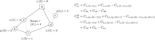Figure 1 illustrates an example where $C_{\mathrm{ir}}^I$ and $C_{\mathrm{ir}}^R$ are calculated.

Figure 1. Illustration of calculating the costs of removing node b from route r and inserting node e at position 5 in route r. Route r is marked with solid lines and the insertion and removal with dotted lines.

A route consisting of the depot and nodes a, b, c and d. The node e is not in the route. We then have the following: i r(1)=a, i r(3)=c, i r(4)=d, i r(5)=0, p r(b)=2 and p * r(e)=5.

Further, the quantity delivered by route r to node i in time period t is denoted $q_{\mathrm{irt}}$, while all other notation has the same meaning as in Section 2.1. The improvement model can be formulated as follows:

(35) $\begin{array}{rl}\min & \sum _{i\in {\mathcal{N}}^{\prime }}\sum _{t\in {\mathcal{T}}^{\prime }}{C}_i^H{s}_{\mathrm{it}}+\sum _{r\in \hat{\mathcal{R}}}\sum _{t\in {\mathcal{T}}^{\prime }}{C}_r^T{y}_{\mathrm{rt}}\\ & -\sum _{r\in \hat{\mathcal{R}}}\sum _{i\in {\mathcal{N}}_r}\sum _{t\in {\mathcal{T}}^{\prime }}{C}_{\mathrm{ir}}^R{x}_{\mathrm{irt}}\\ & +\sum _{r\in \hat{\mathcal{R}}}\sum _{i\in {\overline{\mathcal{N}}}_r}\sum _{t\in {\mathcal{T}}^{\prime }}{C}_{\mathrm{ir}}^I{z}_{\mathrm{irt}}\\ & +\sum _{t\in {\mathcal{T}}^{\prime }}{C}^S{o}_t+\sum _{t\in {\mathcal{T}}^{\prime }}{C}^U{p}_t,\end{array}$(35) (36) $\begin{array}{rlrl}{p}_t& \le P{o}_t,& t\in {\mathcal{T}}^{\prime },& \end{array}$(36) (37) $\begin{array}{rlrl}{s}_{i0}& =I_i,& i\in \mathcal{N},& \end{array}$(37) (38) $\begin{array}{rlrl}{s}_{0t}-s_{0(t-1)}-p_t+\sum _{i\in {\mathcal{N}}^{\prime }}\sum _{r\in \hat{\mathcal{R}}}{q}_{\mathrm{irt}}& =0,& t\in {\mathcal{T}}^{\prime },& \end{array}$(38) (39) $\begin{array}{rlrl}{s}_{\mathrm{it}}-s_{i(t-1)}+D_{\mathrm{it}}-\sum _{r\in \hat{\mathcal{R}}}{q}_{\mathrm{irt}}& =0,& i\in {\mathcal{N}}^{\prime },t\in {\mathcal{T}}^{\prime },& \end{array}$(39) (40) $\begin{array}{rlrl}{L}_i\le s_{\mathrm{it}}& \le U_i,& i\in \mathcal{N},t\in \mathcal{T},& \end{array}$(40) (41) $\begin{array}{rlrl}{q}_{\mathrm{irt}}& \le min(Q,U_i+D_{\mathrm{it}})(1-x_{\mathrm{irt}}),& r\in \hat{\mathcal{R}},i\in {\mathcal{N}}_r,t\in {\mathcal{T}}^{\prime },& \end{array}$(41) (42) $\begin{array}{rlrl}{q}_{\mathrm{irt}}& \le min(Q,U_i+D_{\mathrm{it}})z_{\mathrm{irt}},& r\in \hat{\mathcal{R}},i\in {\overline{\mathcal{N}}}_r,t\in {\mathcal{T}}^{\prime },& \end{array}$(42) (43) $\begin{array}{rlrl}\sum _{i\in {\mathcal{N}}^{\prime }}{q}_{\mathrm{irt}}& \le Q{y}_{\mathrm{rt}},& r\in \hat{\mathcal{R}},t\in {\mathcal{T}}^{\prime },& \end{array}$(43) (44) $\begin{array}{rlrl}\sum _{r\in \hat{\mathcal{R}}:i\in {\mathcal{N}}_r}(y_{\mathrm{rt}}-x_{\mathrm{irt}})+\sum _{r\in \hat{\mathcal{R}}:i\in {\overline{\mathcal{N}}}_r}{z}_{\mathrm{irt}}& \le 1,& i\in {\mathcal{N}}^{\prime },t\in {\mathcal{T}}^{\prime },& \end{array}$(44) (45) $\begin{array}{rlrl}{z}_{\mathrm{irt}}& \le y_{\mathrm{rt}},& r\in \hat{\mathcal{R}},i\in {\overline{\mathcal{N}}}_r,t\in {\mathcal{T}}^{\prime },& \end{array}$(45) (46) $\begin{array}{rlrl}{x}_{\mathrm{irt}}& \le y_{\mathrm{rt}},& r\in \hat{\mathcal{R}},i\in {\mathcal{N}}_r,t\in {\mathcal{T}}^{\prime },& \end{array}$(46) (47) $\begin{array}{rlrl}\sum _{r\in \hat{\mathcal{R}}}{y}_{\mathrm{rt}}& \le V,& t\in {\mathcal{T}}^{\prime },& \end{array}$(47) (48) $\begin{array}{rlrl}{y}_{\mathrm{rt}}& \in \{0,1\},& r\in \hat{\mathcal{R}},t\in {\mathcal{T}}^{\prime },& \end{array}$(48) (49) $\begin{array}{rlrl}{x}_{\mathrm{irt}}& \in \{0,1\},& r\in \hat{\mathcal{R}},i\in {\mathcal{N}}_r,t\in {\mathcal{T}}^{\prime },& \end{array}$(49) (50) $\begin{array}{rlrl}{z}_{\mathrm{irt}}& \in \{0,1\},& r\in \hat{\mathcal{R}},i\in {\overline{\mathcal{N}}}_r,t\in {\mathcal{T}}^{\prime },& \end{array}$(50) (51) $\begin{array}{rlrl}{o}_t& \in \{0,1\},& t\in {\mathcal{T}}^{\prime },& \end{array}$(51) (52) $\begin{array}{rlrl}{q}_{\mathrm{irt}}& \ge 0,& i\in {\mathcal{N}}^{\prime },r\in \hat{\mathcal{R}},t\in {\mathcal{T}}^{\prime },& \end{array}$(52) (53) $\begin{array}{rlrl}{p}_t& \ge 0,& t\in {\mathcal{T}}^{\prime }.& \end{array}$(53)

The objective function (35(35) $\begin{array}{rl}\min & \sum _{i\in {\mathcal{N}}^{\prime }}\sum _{t\in {\mathcal{T}}^{\prime }}{C}_i^H{s}_{\mathrm{it}}+\sum _{r\in \hat{\mathcal{R}}}\sum _{t\in {\mathcal{T}}^{\prime }}{C}_r^T{y}_{\mathrm{rt}}\\ & -\sum _{r\in \hat{\mathcal{R}}}\sum _{i\in {\mathcal{N}}_r}\sum _{t\in {\mathcal{T}}^{\prime }}{C}_{\mathrm{ir}}^R{x}_{\mathrm{irt}}\\ & +\sum _{r\in \hat{\mathcal{R}}}\sum _{i\in {\overline{\mathcal{N}}}_r}\sum _{t\in {\mathcal{T}}^{\prime }}{C}_{\mathrm{ir}}^I{z}_{\mathrm{irt}}\\ & +\sum _{t\in {\mathcal{T}}^{\prime }}{C}^S{o}_t+\sum _{t\in {\mathcal{T}}^{\prime }}{C}^U{p}_t,\end{array}$(35) ) minimises the production, setup, transportation, and inventory holding costs over the entire planning horizon. Constraints (36(36) $\begin{array}{rlrl}{p}_t& \le P{o}_t,& t\in {\mathcal{T}}^{\prime },& \end{array}$(36) )–(40(40) $\begin{array}{rlrl}{L}_i\le s_{\mathrm{it}}& \le U_i,& i\in \mathcal{N},t\in \mathcal{T},& \end{array}$(40) ) are the same as constraints (2(2) $\begin{array}{rlrl}{p}_t& \le P{o}_t,& t\in {\mathcal{T}}^{\prime },& \end{array}$(2) )–(6(6) $\begin{array}{rlrl}{L}_i\le s_{\mathrm{it}}& \le U_i,& i\in \mathcal{N},t\in \mathcal{T},& \end{array}$(6) ) in the original formulation and handle production and inventory. Constraints (41(41) $\begin{array}{rlrl}{q}_{\mathrm{irt}}& \le min(Q,U_i+D_{\mathrm{it}})(1-x_{\mathrm{irt}}),& r\in \hat{\mathcal{R}},i\in {\mathcal{N}}_r,t\in {\mathcal{T}}^{\prime },& \end{array}$(41) ) and (42(42) $\begin{array}{rlrl}{q}_{\mathrm{irt}}& \le min(Q,U_i+D_{\mathrm{it}})z_{\mathrm{irt}},& r\in \hat{\mathcal{R}},i\in {\overline{\mathcal{N}}}_r,t\in {\mathcal{T}}^{\prime },& \end{array}$(42) ) state that a retailer cannot receive any product unless it is visited by a route, while constraints (43(43) $\begin{array}{rlrl}\sum _{i\in {\mathcal{N}}^{\prime }}{q}_{\mathrm{irt}}& \le Q{y}_{\mathrm{rt}},& r\in \hat{\mathcal{R}},t\in {\mathcal{T}}^{\prime },& \end{array}$(43) ) ensure that a vehicle cannot deliver more than its capacity. In addition, constraints (44(44) $\begin{array}{rlrl}\sum _{r\in \hat{\mathcal{R}}:i\in {\mathcal{N}}_r}(y_{\mathrm{rt}}-x_{\mathrm{irt}})+\sum _{r\in \hat{\mathcal{R}}:i\in {\overline{\mathcal{N}}}_r}{z}_{\mathrm{irt}}& \le 1,& i\in {\mathcal{N}}^{\prime },t\in {\mathcal{T}}^{\prime },& \end{array}$(44) ) make sure that a retailer can only be visited by at most one route each time period. The fact that a retailer cannot be added or removed from an unused route is taken care of by constraints (45(45) $\begin{array}{rlrl}{z}_{\mathrm{irt}}& \le y_{\mathrm{rt}},& r\in \hat{\mathcal{R}},i\in {\overline{\mathcal{N}}}_r,t\in {\mathcal{T}}^{\prime },& \end{array}$(45) ) and (46(46) $\begin{array}{rlrl}{x}_{\mathrm{irt}}& \le y_{\mathrm{rt}},& r\in \hat{\mathcal{R}},i\in {\mathcal{N}}_r,t\in {\mathcal{T}}^{\prime },& \end{array}$(46) ), while constraints (47(47) $\begin{array}{rlrl}\sum _{r\in \hat{\mathcal{R}}}{y}_{\mathrm{rt}}& \le V,& t\in {\mathcal{T}}^{\prime },& \end{array}$(47) ) ensure that we do not use more routes in a time period than the number of vehicles. Constraints (48(48) $\begin{array}{rlrl}{y}_{\mathrm{rt}}& \in \{0,1\},& r\in \hat{\mathcal{R}},t\in {\mathcal{T}}^{\prime },& \end{array}$(48) )–(53(53) $\begin{array}{rlrl}{p}_t& \ge 0,& t\in {\mathcal{T}}^{\prime }.& \end{array}$(53) ) define the variable domains.

To keep the transportation cost in the objective function of the improvement model correct, we have to introduce additional constraints to limit the number and type of changes that can be made to a route. Since the cost calculations of an insertion/removal of a node include the previous and subsequent node on the route, we have to ensure that these nodes are still present on the route. Otherwise, some combination of changes, e.g. removing two consecutive nodes, may be evaluated incorrectly in the objective function. The following constraints are added to the formulation to ensure that the transportation costs are correctly calculated:

(54) $\begin{array}{rlrl}{x}_{i_r\left(p_r^{\ast }\right(i)-1),\mathrm{rt}}+x_{i_r\left(p_r^{\ast }\right(i\left)\right),\mathrm{rt}}& \le 2(1-z_{\mathrm{irt}})& r\in \hat{\mathcal{R}},i\in {\overline{\mathcal{N}}}_r,t\in {\mathcal{T}}^{\prime }& \end{array}$(54) (55) $\begin{array}{rlrl}\sum _{i\in {\overline{\mathcal{N}}}_r:p_r^{\ast }\left(i\right)=p}{z}_{\mathrm{irt}}& \le 1& r\in \hat{\mathcal{R}},p\in 1,\dots ,|{\mathcal{N}}_r|+1,t\in {\mathcal{T}}^{\prime }& \end{array}$(55) (56) $\begin{array}{rlrl}{x}_{\mathrm{irt}}+x_{i_r\left(p_r\right(i)+1),\mathrm{rt}}+y_{\mathrm{rt}}& \le 2& r\in \hat{\mathcal{R}},i\in {\mathcal{N}}_r,t\in {\mathcal{T}}^{\prime }& .\end{array}$(56)

Constraints (54(54) $\begin{array}{rlrl}{x}_{i_r\left(p_r^{\ast }\right(i)-1),\mathrm{rt}}+x_{i_r\left(p_r^{\ast }\right(i\left)\right),\mathrm{rt}}& \le 2(1-z_{\mathrm{irt}})& r\in \hat{\mathcal{R}},i\in {\overline{\mathcal{N}}}_r,t\in {\mathcal{T}}^{\prime }& \end{array}$(54) ) state that if a node i that was originally not in route r is inserted, then we must include the nodes that are located before and after the position where node i is inserted into r. Constraints (55(55) $\begin{array}{rlrl}\sum _{i\in {\overline{\mathcal{N}}}_r:p_r^{\ast }\left(i\right)=p}{z}_{\mathrm{irt}}& \le 1& r\in \hat{\mathcal{R}},p\in 1,\dots ,|{\mathcal{N}}_r|+1,t\in {\mathcal{T}}^{\prime }& \end{array}$(55) ) ensure that at most one node, not originally in route r, can be inserted into each position in r. Constraints (56(56) $\begin{array}{rlrl}{x}_{\mathrm{irt}}+x_{i_r\left(p_r\right(i)+1),\mathrm{rt}}+y_{\mathrm{rt}}& \le 2& r\in \hat{\mathcal{R}},i\in {\mathcal{N}}_r,t\in {\mathcal{T}}^{\prime }& .\end{array}$(56) ) make sure that if route r is used, then we cannot remove both node i and its successor, which are both in ${\mathcal{N}}_r$, from the route. Note that apart from the limitations set by constraints (54(54) $\begin{array}{rlrl}{x}_{i_r\left(p_r^{\ast }\right(i)-1),\mathrm{rt}}+x_{i_r\left(p_r^{\ast }\right(i\left)\right),\mathrm{rt}}& \le 2(1-z_{\mathrm{irt}})& r\in \hat{\mathcal{R}},i\in {\overline{\mathcal{N}}}_r,t\in {\mathcal{T}}^{\prime }& \end{array}$(54) )–(56(56) $\begin{array}{rlrl}{x}_{\mathrm{irt}}+x_{i_r\left(p_r\right(i)+1),\mathrm{rt}}+y_{\mathrm{rt}}& \le 2& r\in \hat{\mathcal{R}},i\in {\mathcal{N}}_r,t\in {\mathcal{T}}^{\prime }& .\end{array}$(56) ), any number of insertions and removals are allowed and evaluated correctly, by the improvement model presented above.

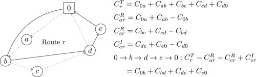
Figure 2 shows the cost calculations of a route in the improvement model. The original route $0\to a\to b\to c\to d\to 0$ is marked with dotted arrows. After solving the improvement model, route r is included in the solution, but nodes a and c have been removed, while node e has been added to the route. The new route is marked with solid arrows.

Figure 2. A route consisting of the depot and nodes a, b, c and d is changed to a route consisting of the depot and nodes b, d and e. The cost of the route is then changed from $C_{0a}+C_{\mathrm{ab}}+C_{\mathrm{bc}}+C_{\mathrm{cd}}+C_{d0}$ to $C_{0b}+C_{\mathrm{bd}}+C_{\mathrm{de}}+C_{e0}$.

An example showing the cost calculations when b, d and e are included in route r and a and c are excluded. The route cost C R r is calculated based on the original route, and the cost of choosing route r and including b, d and e is shown to be correct.

To reduce the solution time of the model we do not generate all insertion possibilities. Defining ${\overline{C}}^N=\max \left\{C_{\mathrm{ir}}^N\right|r\in \hat{\mathcal{R}},i\in {\mathcal{N}}^{\prime }\}$, we only generate $x_{\mathrm{irt}}$ if $C_{\mathrm{ir}}^N\le \gamma {\overline{C}}^N$, where γ is a parameter set a priori. We also only generate the route-indexed variables, i.e. $y_{\mathrm{rt}}$, $x_{\mathrm{irt}}$ and $q_{\mathrm{irt}}$, for the time periods route r appears in the original solution. For instance, if route ρ appears in time period t = 3, then $y_{\mathrm{\rho t}}$, $x_{\mathrm{i\rho t}}$ and $q_{\mathrm{i\rho t}}$ are only generated for t = 3. Lastly, after solving the mathematical model, we run a TSP-heuristic on each of the routes that make up its solution. In our implementation, we use the TSP-solver released by Helsgaun (2009), which is considered to be the fastest implementation of the Lin-Kernighan algorithm (Lin and Kernighan 1973).

3.4. Improvement model with extended route set

In the last part of the matheuristic (line 15 in Algorithm 1), we intensify the search around the most promising solution found by the multi-start phase of the heuristic. We do this by solving the improvement model with an extended route set $\hat{\mathcal{R}}$ for it iterations. The extended route set includes the routes from the current solution in addition to routes found by solving ω CVRPs for each time period. The nodes to visit and the quantities delivered in each CVRP are given by the current solution; however, for each of the ω CVRPs the vehicle capacity is increased or decreased by a given percentage. In each iteration, we update the route set based on the solution of the previous iteration, and the total number of CVRPs in each iteration is bounded by $\omega |{\mathcal{T}}^{\prime }|$. Again, the VRP-heuristic presented in Vidal et al. (2012) is used.

4. Computational experiments

The proposed matheuristic has been evaluated on known benchmark instances for the PRP from the literature. First, we introduce the benchmark instances for the PRP in Section 4.1 and discuss implementation issues and parameter testing in Section 4.2, before presenting the computational results for the PRP in Section 4.3. To demonstrate the versatility of the proposed matheuristic, we have also tested it on benchmark instances for the IRP, and these results are presented in Section 4.4. All computational results have been run on a Xeon Gold 6144 3.5 Ghz computer, and all mathematical models are solved using Gurobi 9.1. The algorithm is coded in C++.

4.1. Benchmark instances and solution methods

Three sets of benchmark instances for the PRP are used in the computational study. The first set was introduced by Archetti et al. (2011) and consists of smaller instances compared with the other instance set. The set consists of three subsets of instances, called A1, A2 and A3, which have six time periods and 14, 50 and 100 retailers, respectively. The instances in A1 have one vehicle available per time period, while the instances in A2 and A3 have an unlimited vehicle fleet. The instances are also divided into four classes where the first class is ‘standard’, the second has high transportation costs, the third has high production costs, and the fourth has no inventory holding costs at the retailers. To differentiate between the classes, we call the subset of instances consisting of class 1 instances in A2 for A2-1, the subset consisting of class 2 instances in A2 for A2-2, and so on. There are in total 1440 instances where 960 of them have an unlimited vehicle fleet. The A1 instances are trivial to solve with an exact method, and we have not done any computational experiments on this subset of instances.

The second set of instances was introduced by Boudia, Louly, and Prins (2007). The set consists of 30 instances with 50 retailers, 30 with 100 retailers, and 30 with 200 retailers. We call them B1, B2, and B3, respectively. They all have 20 time periods and are hence much larger than the instances from Archetti et al. (2011). Moreover, the B1 instances have five vehicles available, the B2 instances have nine vehicles available, while the B3 instances have 13 vehicles available. This set of instances differs from the one proposed by Archetti et al. (2011) in that it has a maximum production capacity per period and an inventory limit at the plant, while the retailers have varying daily demand, but no inventory holding costs.

Another important difference between the two sets of instances is that the production in time period t is not available before time period t + 1 in the instances proposed by Boudia, Louly, and Prins (2007) and does not incur inventory holding costs in time period t. This means that the demand at all nodes in time period t = 1, given that all retailers have an initial inventory of zero, must be managed by the initial inventory at the plant. The instances do not specify what the initial inventories are. Hence, we have adopted the common literature practice of setting the initial inventory at the plant equal to the total retailer demand of time period 1. The initial inventory at the retailers is set to zero. Moreover, the mathematical models presented in Sections 2.1, 3.1 and 3.3 make the production available the same time period. To overcome this fact, have we incorporated the same workaround as Adulyasak, Cordeau, and Jans (2014b) and Manousakis et al. (2022), which sets $o_1=0$. With this workaround, we solve the instances as they were described in Boudia, Louly, and Prins (2007).

The third set of instances was introduced by Adulyasak, Cordeau, and Jans (2014a) and consists of 168 instances. They are based on the above-mentioned Archetti instances and were created since those instances were too large to be solved by an exact method. The instances have either three, six or nine time periods, and the vehicle fleet consists of either two, three or four vehicles. We label this set of instances C to distinguish it from the two other sets. This set of instances uses a stricter inventory policy forcing $q_{\mathrm{it}}+s_{i(t-1)}\le U_i,i\in {\mathcal{N}}^{\prime },t\in {\mathcal{T}}^{\prime }$ and it is the set of instances that has been used the least in the literature.

To evaluate our results, we have compared them with the results presented in other papers that have solved the same instances. We have tried to gather the results of all relevant methods. The matheuristic proposed by Archetti et al. (2011) has not been included since, according to Solyalı and Süral (2017), it has an error in its implementation. In addition, the results of Russell (2017) have also been left out. The authors of Manousakis et al. (2022) report that they were unable to re-create the reported objective values in B3 from the solution files which they received from the author of the above-mentioned paper. Hence, it is likely that different assumptions or objective value calculations have been used in Russell (2017). We have not been successful in our attempts to contact the author of Russell (2017). If we had included the results in our evaluation, Russell (2017) would have had the BKS for four of the Archetti instances, four of the B1 instances and ten of the B3 instances.

In general, the more recently published papers have better results than the older ones. Some of the methods presented have focussed on the smaller instances from Archetti et al. (2011), while others have focussed on the larger instances from Boudia, Louly, and Prins (2007). The instances from Adulyasak, Cordeau, and Jans (2014a) have mainly been used by exact methods. However, the methods and results have all used different CPUs and software, hence making a fair comparison of the time consumption is hard. In Table 1, we summarise essential features of all solution methods. A complete overview of the instances used to test each method can be found in Table 2.

Table 1. An overview of all solution methods for the PRP.

Reference	Abbreviation	Sol	CPU	#Threads	Solver
Schenekemberg et al. (2021)	SSPG-BC	E	Intel(R) Xeon(R) 2.60 GHz	6	Gurobi 8.1
Adulyasak, Cordeau, and Jans (2014a)	ACJ-BC	E	AMD Opteron 2.40 GHz	8	CPLEX 12.3
Boudia and Prins (2009)	BP-MA	H	2.30 GHz PC	1	–
Adulyasak, Cordeau, and Jans (2014b)	ACJ-ALNS-500	H	2.10 GHz Duo CPU PC	Def	CPLEX 12.2
	ACJ-ALNS-1000	H
Qiu et al. (2018)	QWXFP-VNS	H	Intel Core 2 Duo P8600 2.40 GHz	Def	CPLEX 12.6
Absi et al. (2015)	AADF-VRP	M	Xeon 2.67 GHz PC	Def	CPLEX 12.1
	AADF-MTSP	M
Solyalı and Süral (2017)	SS-M	M	2.40 GHz PC	12	CPLEX 12.5
Chitsaz, Cordeau, and Jans (2019)	CCJ-M	M	Xeon X5650 2.67 GHz	1	CPLEX 12.6
Li et al. (2019)	LCCF-M	M	Intel Core i7 2.5 GHz	Def	CPLEX 12.6
Avci and Yildiz (2019)	AY-M	M	Intel Core i5-760X 4.00 GHz	Def	CPLEX 12.6
Manousakis et al. (2022)	MKKZ-M	M	Intel Core i7-7700 3.60 GHz	1	Gurobi 9.0.2
This paper	VACS-M	M	Xeon Gold 6144 3.5 GHz	1	Gurobi 9.1

Note: Def = Default, Sol = Solution method, E = Exact method, H = Heuristic, M = Matheuristic.

Table 2. The number of instances solved by each solution method.

			SSPG-BC	ACJ-BC	BP-MA	ACJ-ALNS-500	ACJ-ALNS-1000	QWXFP-VNS	AADF-VRP	AADF-MTSP	SS-M	CCJ-M	LCCF-M	AY-M	MKKZ-M	VACS-M
Set	V	Size	E	E	H	H	H	H	M	M	M	M	M	M	M	M
A2-1	∞	120	–	–	–	120	120	120	120	120	120	120	120	120	120	120
A2-2	∞	120	–	–	–	120	120	120	120	120	120	120	120	120	120	120
A2-3	∞	120	–	–	–	120	120	120	120	120	120	120	120	120	120	120
A2-4	∞	120	–	–	–	120	120	120	120	120	120	120	120	120	120	120
A3-1	∞	120	–	–	–	120	120	120	120	120	120	120	120	120	120	120
A3-2	∞	120	–	–	–	120	120	120	120	120	120	120	120	120	120	120
A3-3	∞	120	–	–	–	120	120	120	120	120	120	120	120	120	120	120
A3-4	∞	120	–	–	–	120	120	120	120	120	120	120	120	120	120	120
B1	5	30	30	–	30	30	30	30	30	30	30	30	30	–	30	30
B2	9	30	30	–	30	30	30	30	30	30	30	30	30	–	30	30
B3	13	30	–	–	30	30	–	30	30	30	30	30	30	–	30	30
C	2–4	168	168	168	–	168	–	–	–	–	–	–	–	–	–	168

Note: V = Number of vehicles, E = Exact method, H = Heuristic, M = Matheuristic.

When comparing our solution methods throughout this paper, we have used the one-tailed Wilcoxon signed-rank test (Wilcoxon 1945), a nonparametric test to compare two independent groups, to ensure that the median of the difference of the objective values between our proposed method (X) and the method we compare with (Y) is significantly different from zero. In the test, we evaluate two hypotheses, the null-hypothesis $H_0$, and the alternative hypothesis $H_1$, defined as follows: $\begin{array}{rl}{H}_0& :\mathrm{median}(X-Y)=0,\\ H_1& :\mathrm{median}(X-Y)>0,\end{array}$where median(X−Y) is the median of the pairwise differences in objective value over the test instances. Rejecting both hypotheses leads to the conclusion that our method obtains better solutions than the method it is compared with. We use a significance level $\alpha =0.01$.

4.2. Algorithmic implementation and parameters

The used parameter values were obtained by running preliminary tests where different parameter configurations were tested and compared. We would like to point at that the proposed method can be considered to be more of a framework than an exact recipe of how to solve the problem. Hence, we did not put considerable effort into tuning the parameters and better configurations are likely to exist. Practitioners solving similar problems should scale the parameters according to their needs and constraints. The parameter values used in this computational study are presented in Table 3. The instances differ in size and complexity, and different parameter settings are thus more suitable for specific subsets of instances. However, to avoid overfitting, we have used the same parameter settings for all instances, except for ω, which is different for B3.

Table 3. Parameter values.

Name	Value
α	1/V
β	0.975
γ	0.25
δ	4
ω	3 ($-3\mathrm{\%},+3\mathrm{\%},+6\mathrm{\%}$)
${ϵ}_1$	1
${ϵ}_2$	3
${ϵ}_3$	3
it	5
Time Limit: Initial solution	$0.5\left|N\right|$
Time Limit: Improvement model 1	$\left|N\right|$
Time Limit: Improvement model 2	$10\left|T^{\prime }\right|+0.5\left|N\right|$

The parameter α is the factor we multiply the cost $C^{\mathrm{TSP}}$ with. Here, V is the number of vehicles in the instance. The number of vehicles is set to $\underset{t\in {\mathcal{T}}^{\prime }}{max}\left(2\sum _{i\in {\mathcal{N}}^{\prime }}{D}_{\mathrm{it}}\right)/\left(Q|T^{\prime }|\right)$ for instances where the vehicle fleet is unlimited. The parameters β and γ are the factors that Q and ${\overline{C}}^N$ are multiplied with, and δ is the number of consecutive times we run the improvement model in each iteration of the multi-start phase of the heuristic. The parameter ω denotes the number of CVRPs solved per time period in each iteration when we solve the improvement model with an extended route set. Each time we solve a CVRP, the capacity of the vehicles is altered. First, it is decreased by 3%, then increased by 3%, and finally increased by 6%. However, for B3, we only solve one VRP per time period in each iteration, increasing the capacity by 3%. This is because the improvement model becomes too large and difficult to solve if too many routes are added to $\hat{\mathcal{R}}$ in B3.

The parameters ${ϵ}_1$, ${ϵ}_2$ and ${ϵ}_3$ give the number of times we run the three different differentiation techniques, and it is the maximum number of iterations when we solve the improvement model with an extended route set. ‘Time Limit: Initial solution’ refers to the time limit in seconds put on solving the mathematical model used to solve the production subproblem, and ‘Improvement model 1’ refers to the improvement model in the multi-start phase of the matheuristic. In contrast, ‘Improvement model 2’ refers to the improvement model when using an extended route set. Time limits have been enforced due to the fact that this is a matheuristic and there is no reason to spend time on closing the optimality gap when it has little impact on the final solution.

4.3. Computational results for the production routeing problem

In this section, the proposed matheuristic is compared with the benchmark solution methods for the PRP. First, we present the results on the benchmark instances from Adulyasak, Cordeau, and Jans (2014a). Most of these instances are solved to proven optimality in the literature. Second, we present the comparison on the benchmark instances from Archetti et al. (2011), and finally on the benchmark instances from Boudia, Louly, and Prins (2007). The detailed computational results, and solutions, can be found at http://axiomresearchproject.com/publications/.

4.3.1. Test results on the Adulyasak instances

The results of running the proposed matheuristic (denoted VACS-M) on each of the 168 instances from Adulyasak, Cordeau, and Jans (2014a) are compared with existing results from the literature. All the computational results are summarised in Table 4. Here, Gap refers to the average gap in percentage which is calculated for each instance as the difference between the objective value obtained by a method and the current best-known objective value (not including this paper), divided by the best-known objective value. Further, Time refers to the average time in seconds over a subset of instances, #BKS refers to the number of best-known solutions and the number within the parentheses refers to the number of (known) optimal solutions found. In addition, the VACS-M column New shows the number of BKS that are new to the literature and have a strictly better objective value than the old BKS.

Table 4. The average results for the Adulyasak instances.

		ACJ-BC			ACJ-ALNS			SSPG-BC			VACS-M
Set	Size	Gap	Time	#BKS	Gap	Time	#BKS	Gap	Time	#BKS	Gap	Time	#BKS	New
C-10	24	0.00	64	24 (24)	1.03	–	2 (2)	0.00	13	24 (24)	0.32	5	9 (9)	0
C-15	24	0.01	7734	20 (20)	1.41	–	2 (2)	0.00	2540	24 (20)	0.59	12	4 (4)	0
C-20	24	0.01	4084	23 (22)	1.37	–	2 (2)	0.00	1030	24 (24)	0.20	8	9 (9)	0
C-25	24	0.06	10,535	20 (20)	1.39	–	1 (1)	0.00	1984	23 (22)	0.29	18	6 (6)	0
C-30	24	0.37	20,621	14 (14)	1.61	–	0 (0)	0.00	5787	24 (16)	0.57	73	2 (2)	0
C-35	16	0.16	20,563	11 (11)	1.97	–	0 (0)	0.00	4800	16 (13)	0.39	18	2 (2)	0
C-40	16	0.27	29,370	7 (7)	1.05	–	0 (0)	0.00	9860	12 (7)	0.16	17	5 (1)	3
C-45	8	0.34	27,798	5 (5)	1.15	–	1 (1)	0.03	12,652	4 (2)	0.59	12	2 (1)	1
C-50	8	0.04	21,318	5 ( 5)	1.60	–	0 (0)	0.00	6404	7 (6)	0.53	11	2 (1)	1
Sum/Avg.		0.12	13,243	129 (128)	1.39	–	8 (8)	0.00	3926	158 (134)	0.39	21	41 (35)	5

Note: #BKS = Number of best-known solutions.

VACS-M finds 35 optimal solutions out of 168 instances and 41 BKS where five of them have a strictly improving objective value. In addition, an average gap of 0.39% is noticeably better than ACJ-ALNS which is the only other heuristic that has solved this set of instances. For each subset of instances, the one-tailed Wilcoxon signed-rank test indicates that VACS-M is statistically significantly better than ACJ-ALNS. Thus, the results indicate that VACS-M produces close to optimal solutions using less than 0.5% of the computing time used by exact methods. The solution times of ACJ-ALNS were unfortunately not reported by the authors.

4.3.2. Test results on the Archetti instances

The results of running the proposed matheuristic (denoted VACS-M) on each of the 960 multi-vehicle instances from Archetti et al. (2011) are compared with existing results from the literature. All the computational results are summarised in Tables 5–7. In Table 5, the average gaps of each solution method is presented. Again, the solution gap obtained by a method for a given instance is calculated as the difference between the objective value obtained with the method and the current best-known objective value (not including this paper), divided by the best-known objective value. In Table 6 the number of BKSs are presented. Finally, Table 7 shows the average computing times for each solution method.

Table 5. The average gaps in percentage for the Archetti instances.

			ACJ-ALNS-500	ACJ-ALNS-1000	QWXFP-VNS	AADF-VRP	AADF-MTSP	SS-M	CCJ-M	LCCF-M	AY-M	MKKZ-M	VACS-M
Set	V	Size	H	H	H	M	M	M	M	M	M	M	M
A2-1	∞	120	1.36	1.35	0.26	0.38	1.30	0.27	0.16	0.21	0.18	0.02	0.04
A2-2	∞	120	0.22	0.22	0.08	0.10	0.14	0.06	0.06	0.05	0.06	0.00	0.02
A2-3	∞	120	4.63	4.39	0.87	1.83	3.57	0.92	0.62	0.82	0.78	0.06	0.15
A2-4	∞	120	0.36	0.35	0.13	0.25	0.62	0.21	0.13	0.18	0.17	0.06	$\mathbf{\text{-0.01}}$
A3-1	∞	120	1.10	1.05	0.23	0.27	1.91	0.12	0.23	0.08	0.07	0.19	$\mathbf{\text{-0.05}}$
A3-2	∞	120	0.17	0.16	0.08	0.06	0.14	0.04	0.04	0.03	0.05	0.00	0.00
A3-3	∞	120	4.16	3.97	0.62	1.54	4.13	0.46	1.38	0.47	0.55	0.37	$\mathbf{\text{-0.18}}$
A3-4	∞	120	0.37	0.35	0.10	0.26	0.72	0.07	0.08	0.06	0.11	0.14	$\mathbf{\text{-0.08}}$
Average			1.54	1.48	0.30	0.59	1.57	0.27	0.34	0.24	0.24	0.11	$\mathbf{\text{-0.01}}$

Note: $V=$ Number of vehicles, H = Heuristic, M = Matheuristic.

Table 6. The number of best-known solutions (BKSs) for the Archetti instances.

			ACJ-ALNS-500	ACJ-ALNS-1000	QWXFP-VNS	AADF-VRP	AADF-MTSP	SS-M	CCJ-M	LCCF-M	AY-M	MKKZ-M	VACS-M
Set	V	Size	H	H	H	M	M	M	M	M	M	M	M
A2-1	∞	120	0	0	0	0	0	2	22	2	9	57	62 (41)
A2-2	∞	120	0	0	0	0	0	0	1	2	0	99	18 (18)
A2-3	∞	120	0	0	0	0	0	2	7	0	3	61	58 (52)
A2-4	∞	120	0	0	2	0	1	0	4	0	4	69	44 (41)
A3-1	∞	120	0	0	0	0	0	2	4	1	5	6	102 (102)
A3-2	∞	120	0	0	0	3	0	0	3	2	0	57	55 (55)
A3-3	∞	120	0	0	0	0	0	2	0	2	2	19	95 (95)
A3-4	∞	120	0	0	0	1	0	0	6	3	0	29	82 (81)
Total			0	0	2	4	1	8	47	12	23	397	516 (485)

Note: The number within parentheses refers to the number of strictly improving solutions. $V=$ Number of vehicles, H = Heuristic, M = Matheuristic.

Table 7. The average computing time in seconds for the Archetti instances.

			ACJ-ALNS-500	ACJ-ALNS-1000	QWXFP-VNS	AADF-VRP	AADF-MTSP	SS-M	CCJ-M	LCCF-M	AY-M	MKKZ-M*	VACS-M
Set	V	Size	H	H	H	M	M	M	M	M	M	M	M
A2-1	∞	120	29	50	25	23	315	16	400	43	89	1513	130
A2-2	∞	120	28	50	21	23	288	14	344	37	78	1563	103
A2-3	∞	120	24	43	25	26	335	16	309	39	78	1832	156
A2-4	∞	120	26	44	28	26	330	25	434	42	84	1409	142
A3-1	∞	120	136	249	85	86	514	324	2125	169	187	10,174	857
A3-2	∞	120	125	221	73	76	497	51	1947	132	102	11,073	508
A3-3	∞	120	107	191	73	75	509	350	1461	145	290	11,013	978
A3-4	∞	120	108	189	84	87	507	125	2213	160	176	11,760	605
Average			73	130	52	53	412	115	1154	95	135	6292	435

Note: $V=$ Number of vehicles, H = Heuristic, M = Matheuristic, * = estimated time

It is clear from Table 5 that VACS-M has the best average gap over all Archetti instances. However, we can see that the differences are rather small between the different methods. This is primarily because most of the instances have setup and production costs that are significantly larger than the transportation costs. Hence, only improving the routeing decisions does not necessarily lead to a significantly better solution in terms of gap. With this in mind, we can conclude that VACS-M finds slightly better solutions, on average, compared with the other methods. This is backed up by the results of the one-tailed Wilcoxon signed-rank test for all Archetti instances that states that VACS-M is statistically signficantly better than MKKZ (the second best method). However, MKKZ-M finds, on average, better solutions for the A2 instances. The reason why MKKZ-M performs better on these instances than VACS-M is probably because fewer vehicles are used on average in the A2 instances than in the A3 instances. Generally, VACS-M performs better on instances that require a higher number of vehicles.

Table 6 presents the number of BKSs found by each solution method. The VACS-M column includes the number of solutions that have a strictly improving objective value and is displayed within parentheses. We can see that VACS-M finds the BKS in 516 out of 960 instances which is significantly more than any other method. In fact, VACS-M finds a strictly improving solution in over fifty percent of the 960 instances. Interestingly, the two subsets of instances where VACS-M has the lowest number of BKSs are A2-2 and A3-2. These are the instances with high transportation costs. This indicates that our proposed matheuristic performs worse when the transportation costs are high. A possible explanation for this is that since the proposed matheuristic does not consider the location of retailers in the production subproblem, it may therefore serve retailers that are geographically very spread in the same time period. This may lead to long vehicle routes, which is expensive when the transportation costs are high.

Table 7 displays the average computing time for all solution methods. Manousakis et al. (2022) only report the computing time of the individual restart that produced their best solution and not the total running time of their entire matheuristic consisting of 100 restarts. Unfortunately, the authors could not provide their total running times upon request, so to estimate their running times, we multiplied their reported times by 100. It is clear from the table that VACS-M is significantly slower than the fastest solution methods. However, the reported times of VACS-M are still reasonable considering the complexity of the problem instances, and the extra time spent is worth it considering the improvement in solution quality. Further, the reported time is less than 10% of Manousakis et al. (2022) which is the second best solution method, both in terms of average gap and BKSs, and less than 50% of Chitsaz, Cordeau, and Jans (2019) which has the third most BKSs.

4.3.3. Test results on the Boudia instances

The results of running the proposed matheuristic (denoted VACS-M) on each of the 90 multi-vehicle instances proposed by Boudia and Prins (2009) are compared with existing results from the literature. All the computational results are summarised in Tables 8–10. In Table 8, the average gap of each solution method is presented. Table 9 shows the number of BKSs. Finally, in Table 10 the average computing times for each solution method are presented.

Table 8. The average gap in percentage for the Boudia instances.

			SSPG-BC	BP-MA	ACJ-ALNS-500	ACJ-ALNS-1000	QWXFP-VNS	AADF-VRP	AADF-MTSP	SS-M	CCJ-M	LCCF-M	MKKZ-M	VACS-M
Set	V	Size	E	H	H	H	H	M	M	M	M	M	M	M
B1	5	30	3.23	15.73	2.19	2.08	1.75	2.70	2.46	1.06	1.81	1.32	0.00	0.02
B2	9	30	12.46	13.99	1.62	1.60	1.26	1.50	1.97	0.71	1.86	0.55	0.07	−0.54
B3	13	30	–	17.33	2.70	–	1.27	1.43	3.02	3.34	1.25	0.41	0.20	−0.94
Average			7.84	15.68	2.17	1.84	1.42	1.87	2.48	1.70	1.64	0.76	0.09	−0.49

Note: $V=$ Number of vehicles, E = Exact method, H = Heuristic, M = Matheuristic, – = The instances are not solved by the solution method.

Table 9. The number of best-known solutions (BKSs) for the Boudia instances.

			SSPG-BC	BP-MA	ACJ-ALNS-500	ACJ-ALNS-1000	QWXFP-VNS	AADF-VRP	AADF-MTSP	SS-M	CCJ-M	LCCF-M	MKKZ-M	VACS-M
Set	V	Size	E	H	H	H	H	M	M	M	M	M	M	M
B1	5	30	0	0	0	0	0	0	0	0	0	0	15	15 (15)
B2	9	30	0	0	0	0	0	0	0	0	0	0	0	30 (30)
B3	13	30	–	0	0	–	0	0	0	0	0	0	0	30 (30)
Total			0	0	0	0	0	0	0	0	0	0	15	75 (75)

Note: $V=$ Number of vehicles, E = Exact method, H = Heuristic, M = Matheuristic, – = The instances are not solved by the solution method.

Table 10. The average computing time in seconds for the Boudia instances.

			ASSPG-BC	BP-MA	ACJ-ALNS-500	ACJ-ALNS-1000	QWXFP-VNS	AADF-VRP	AADF-MTSP	SS-M	CCJ-M	LCCF-M	MKKZ-M*	VACS-M
Set	V	Size	E	H	H	H	H	M	M	M	M	M	M	M
B1	5	30	14,400	117	298	481	488	298	481	2464	3559	277	31,750	1543
B2	9	30	14,400	976	1405	1570	1767	1405	1570	7487	9811	493	82,194	4784
B3	13	30	–	1148	5794	–	5884	4197	19,270	16,365	15,891	614	202,111	8712
Average			14,400	747	2499	1025	2713	1977	7107	8772	9754	461	105,351	5013

Note: $V=$ Number of vehicles, E = Exact method, H = Heuristic, M = Matheuristic, *= estimated time, – = The instances are not solved by the solution method.

Table 8 shows the average gap of each solution method for all subsets of the Boudia instances. The average gaps are calculated the same way as in Table 5. MKKZ-M has the best average gap on the B1 instances, while VACS-M has the best average gap on the B2 and B3 instances. The results of the one-tailed Wilcoxon signed-rank test state that the results of VACS-M are statistically significantly better than the results of MKKZ for B2 and B3. However, for B1 there is no significant difference, and the $H_0$ hypothesis cannot be rejected. Overall, we can see that VACS-M has a lower average gap than all other solution methods and that its performance relative to the other solution methods gets better as the number of retailers increases.

Table 9 presents the number of BKSs for all solution methods. VACS-M finds the BKS for 75 out of 90 instances, where all of them are strictly improving the previous BKS. In fact, VACS-M improves the BKS for all the B2 and B3 instances. The only solution method besides VACS-M that has any BKSs is MKKZ-M.

Table 10 presents the average computing time for all solution methods for the Boudia instances. VACS-M spends on average 5013 seconds over all instances. This is reasonable considering the complexity and size of the instances. In addition, this is also competitive compared with the other solution methods, especially since VACS-M is superior with respect to solution quality. In fact, MKKZ-M, which is the second-best solution method in terms of solution quality, spends over 100,000 seconds. This is, however, as in Table 7, an estimate since the authors of Manousakis et al. (2022) do not provide their total solution times.

4.4. Test results on the inventory routeing problem

We have also tested the matheuristic on the large multi-vehicle benchmark instances for the IRP released by Archetti et al. (2012). These instances were originally designed for the single-vehicle case, but are adapted to the multi-vehicle version by dividing the vehicle capacity by the number of vehicles and rounding to the nearest integer. They consist of 240 instances with six time periods, where one-third of the instances has 50 retailers, another third has 100 retailers, and the last third has 200 retailers. The number of vehicles differs between two and five. We have compared our results with Coelho and Laporte (2013) (CL-BC), Archetti, Boland, and Speranza (2017) (AR-H2), Chitsaz, Cordeau, and Jans (2019) (C-M), Guimarães et al. (2020) (G-BC), Manousakis et al. (2020) (M-BC), Vadseth, Andersson, and Stålhane (2021) (V-M), Archetti et al. (2021) (AR-H3) and Solyalı and Süral (2022). The results of Achamrah, Riane et al. (2022) have not been included since their results are inconsistent with the literature and super-optimal solutions have been reported. The authors have at a later stage corrected their results (Achamrah, Limbourg et al. 2022).

To test the proposed matheuristic on the multi-vehicle IRP we have excluded differentiation technique 2 described in Section 3.2 since there are no production decisions in the IRP. In addition, the mathematical models in Section 3.1 and Section 3.3 must be updated. We do so by setting $o_t=1$ and $p_t$ equal to the constant production rate for all $t\in {\mathcal{T}}^{\prime }$. In addition, we set $C^S$ and $C^U$ equal to zero. The results are presented in Tables 11–13, and show the average gap, number of BKSs, and average computing time, respectively.

Table 11. The average gap in percentage for the IRP.

			CL-BC	AR-H2	C-M	G-BC	M-BC	V-M	AR-H3	S-M	VACS-M
Retailers	V	Size	E	M	M	E	E	M	M	M	M
50	2	20	2.57	1.76	3.59	0.11	0.24	1.06	3.89	0.81	2.35
	3	20	19.97	2.34	3.00	2.47	0.80	0.38	3.65	0.34	0.94
	4	20	–	2.67	2.38	3.91	0.79	0.17	3.31	1.16	−0.02
	5	20	–	4.25	2.84	5.55	0.64	0.05	3.40	1.54	−0.29
Average:			11.27	2.75	2.95	3.01	0.62	0.41	3.56	0.96	0.67
100	2	20	138.22	6.41	2.26	3.49	0.51	0.75	5.76	0.44	1.19
	3	20	216.39	6.30	2.90	12.68	1.07	0.64	4.68	0.14	1.22
	4	20	–	9.70	1.71	21.88	1.15	0.18	5.98	0.90	0.24
	5	20	–	8.20	2.00	27.57	1.53	0.08	4.99	1.57	−0.19
Average:			177.30	7.65	2.22	16.41	1.07	0.41	5.35	0.76	0.61
200	2	20	–	5.67	1.52	10.48	–	0.88	6.45	0.01	1.29
	3	20	–	9.10	2.26	19.90	–	0.65	9.93	0.07	0.74
	4	20	–	9.41	1.31	35.38	–	0.14	8.45	0.84	0.23
	5	20	–	9.56	0.94	46.87	–	0.19	7.68	1.20	−0.24
Average:			–	8.43	1.51	28.16	–	0.46	8.05	0.53	0.51
Total Average:			94.29	6.28	2.23	15.86	0.84	0.43	5.66	0.75	0.62

Note: $V=$ Number of vehicles, E = Exact method, H = Heuristic, M = Matheuristic, – = The instances are not solved by the solution method.

Table 12. The number of best-known solutions (BKSs) for the IRP.

			CL-BC	AR-H2	C-M	G-BC	M-BC	V-M	AR-H3	S-M	VACS-M
Retailers	V	Size	E	M	M	E	E	M	M	M	M
50	2	20	0	0	0	8	7	2	0	3	1 (1)
	3	20	0	0	0	0	3	6	0	9	3 (3)
	4	20	–	0	0	0	2	6	0	0	13 (12)
	5	20	–	0	0	0	0	8	0	0	12 (12)
Sum:			0	0	0	8	12	22	0	12	29 (28)
100	2	20	0	0	0	0	8	5	0	6	1 (1)
	3	20	0	0	0	0	3	4	0	10	3 (3)
	4	20	–	0	0	0	2	7	0	3	8 (8)
	5	20	–	0	0	0	0	10	0	1	9 (9)
Sum:			0	0	0	0	13	26	0	20	21 (21)
200	2	20	–	0	0	0	–	2	0	17	1 (1)
	3	20	–	0	0	0	–	4	0	15	1 (1)
	4	20	–	0	0	0	–	9	0	4	7 (7)
	5	20	–	0	0	0	–	5	0	1	14 (14)
Sum:			–	0	0	0	–	20	0	37	23 (23)
Total Sum:			0	0	0	8	25	68	0	69	73 (72)

Note: $V=$ Number of vehicles, E = Exact method, H = Heuristic, M = Matheuristic, – = The instances are not solved by the solution method.

Table 13. The average computing time in seconds for the IRP.

			CL-BC	AR-H2	C-M	G-BC	M-BC	V-M	AR-H3	S-M	VACS-M
Retailers	V	Size	E	M	M	E	E	M	M	M	M
50	2	20	86,400	5640	435	7200	7200	166	131	408	27
	3	20	86,400	5729	546	7200	7200	318	2840	3633	53
	4	20	–	5867	519	7200	7200	514	3543	3646	146
	5	20	–	5924	574	7200	6952	544	4837	3659	334
Average:			86,400	5790	519	7200	7138	385	2835	2836	140
100	2	20	86,400	2357	2406	7200	7200	270	93	426	56
	3	20	86,400	3690	2394	7200	7201	588	883	3316	90
	4	20	–	2705	2270	7200	7201	794	2980	3662	167
	5	20	–	3129	2513	7200	7200	1033	4989	3677	262
Average:			86,400	2970	2396	7200	7200	671	2236	2770	144
200	2	20	–	4201	14,128	7200	–	613	338	2723	216
	3	20	–	4201	9688	7200	–	963	534	6829	288
	4	20	–	4200	12,606	7200	–	1446	1316	7500	501
	5	20	–	4201	13,495	7200	–	1892	2483	7524	677
Average:			–	4201	12,480	7200	–	1229	1168	6144	421
Total Average:			86,400	4320	5131	7200	7169	762	2080	3917	235

Note: $V=$ Number of vehicles, E = Exact method, H = Heuristic, M = Matheuristic, – = The instances are not solved by the solution method.

It is clear from Table 11 that VACS-M has the second-best average gap of the solution methods tested on these instances, and that it performs better as the number of available vehicles increases. For five vehicles, VACS-M has the best gap for all numbers of retailers (which is statistically significant according to the one-tailed Wilcoxon signed-rank test). This indicates that our proposed method performs best when many vehicles are available, which is probably due to how the initialisation process works. Since the production subproblem does not consider the geographical placement of retailers, it may serve retailers that are geographically very spread in the same time period. Having more vehicles available therefore reduces the chance of having to construct long routes that cover undesirably large distances in order to serve the given retailers.

Table 12 shows that VACS-M finds the BKS in 73 out of 240 instances. In addition, 72 of these are strictly improving. This means that VACS-M finds more BKS than any other solution method. Again, we can see that it is on the instances with four and five vehicles that VACS-M performs best.

Table 13 gives the average computing time for all solution methods. Even though it is hard to compare the different methods since different computers and solvers have been used, we can see that both VACS-M and V-M use less than 40% of the computing time of any other method tested on these instances. It is improbable that this is only due to differences in CPU speed. Furthermore, VACS-M and V-M have been run on the same computer, where the only difference is that VACS-M uses Gurobi 9.1 instead of 9.0. We conclude that VACS-M is about three times faster than V-M, while providing, on average, almost the same solution quality.

4.5. Analysis of the different components and recommendations

To assess the importance of the different components of the matheuristic have we tested different configurations. We have run the matheuristic without the intensification phase, without differentiation technique 1, without differentiation technique 2 and with no differentiation techniques and compared the results with the full algorithm. This has been done for all Boudia instances and ten instances for each class of Archetti instances for both 50 retailers and 100 retailers. The results are highlighted in Table 14.

Table 14. The reduction in solution quality, given in percentage, if different components of the matheuristic are removed.

Set	V	Size	No intensification phase	No diff. technique 1	No diff. technique 2	No diff. technique
A1-1	∞	10	0.06	0.03	0.00	0.04
A1-2	∞	10	0.00	0.01	0.00	0.01
A1-3	∞	10	0.16	0.00	2.45	2.44
A1-4	∞	10	0.04	0.10	0.00	0.45
A2-1	∞	10	0.03	0.02	0.00	0.02
A2-2	∞	10	0.01	0.00	0.00	0.00
A2-3	∞	10	0.14	0.03	1.49	1.41
A2-4	∞	10	0.07	0.05	0.00	0.05
Average			0.06	0.03	0.49	0.55
B1	5	30	0.36	0.31	0.03	0.35
B2	9	30	0.06	0.32	0.00	0.42
B3	13	30	0.07	0.38	0.02	0.38
Average			0.16	0.33	0.02	0.38
Total Average			0.07	0.11	0.14	0.26

Note: $V=$ Number of vehicles, diff. = differentiation.

Here, all numbers are percentages and represent the solution gap between the full matheuristic and the different configurations. The solution gap is calculated as the solution value of a configuration minus the solution value of the full matheuristic divided by the solution value of the full matheuristic. First of all, we can see that the percentages are quite small. This is again mainly due to the fact that the setup and production costs are so high that the routeing costs have little impact on the total costs. However, our matheuristic is still able to outperform other solution methods in most instances without the intensification phase or differentiation techniques. Hence, the solution found by the first iteration is often of very high quality, and the solutions found from applying the differentiation techniques only have a marginal effect. Further, we can see that differentiation technique 1 is the most important one and that differentiation technique 2 is primarily needed when the production costs are high (which is the case for the third class of Archetti instances). The intensification phase improves the solution, but its contribution to the overall solution is marginal and can hence be dropped if computing time is an issue. In addition, sometimes a better solution is obtained without using any differentiation techniques since the intensification phase can lead to a better solution even if the starting solution is worse.

The key takeaway for a practitioner or someone else who needs to solve a production routeing problem is that the matheuristic works well without multiple restarts. However, if one needs to find a solution that is as good as possible and time is not critical – then the whole matheuristic should be used. Further, if the problem contains specific structures, this should be incorporated into a differentiation technique. For instance, differentiation technique 2 is often not needed, but is very advantageous for specific instances. In conclusion, we can see from Table 14 that all parts of the matheuristic contribute to the overall performance and, hence, we recommend using the matheuristic as described and adding extra differentiation techniques if relevant.

5. Concluding remarks and future research

In this paper, we propose a novel multi-start route improving matheuristic for the well-studied production routeing problem (PRP). A feasible solution to the PRP is created in each restart by first solving a relaxed subproblem of the problem. This subproblem relaxes all routeing decisions and gives a smaller mathematical model than what has previously been used in the literature. Thereafter, a capacitated vehicle routeing problem (CVRP) is solved for each time period to construct the full starting solution. The routes from this solution are then used in a novel path-flow-inspired improvement model that allows us to make alterations to the routes. This improvement phase avoids the shortcomings of the traditional decomposition used in the PRP literature since the model allows us to consider multiple changes to all the routes in the model simultaneously, while at the same time evaluating the effect of these changes on the production and distribution decisions. All these changes are evaluated exactly using the full objective function of the problem, rather than an approximate one. Finally, the most promising solution from the different restarts is further improved by solving the above-mentioned improvement model with an extended route set for multiple iterations.

Computational results show that the matheuristic provides high-quality solutions on benchmark instances for both the PRP and inventory routeing problem (IRP). The computational results for the set of smaller benchmark instances released by Adulyasak, Cordeau, and Jans (2014a) indicate that the proposed method produces close to optimal solutions within a small fraction of the computing time used by exact methods. For the set of multi-vehicle benchmark instances released by Archetti et al. (2011) it finds the best-known solution (BKS) for 516 out of 960 instances, and for the larger and different instance set released by Boudia, Louly, and Prins (2007) it finds the BKS for 75 out of 90 instances. Further, for the set of multi-vehicle IRP instances released by Archetti et al. (2012) our matheuristic finds the BKS for 73 out of 240 instances. Our method spends considerably shorter computing times on the IRP instances than all other comparable methods. Overall, this is significantly better in terms of solution quality compared with all other known solution methods, and the excellent performance on different sets of instances highlights the versatility of our proposed method.

An analysis of the different components of the matheuristic shows that the initial iteration often provides high-quality solutions and that multiple restarts sometimes only marginally improve the solutions. A practitioner, or someone who solves a production routeing problem, can therefore choose not to use the entire matheuristic if computing time is an issue. However, the best results are obtained by using the entire algorithm. We have tested the matheuristic on the standard PRP, and an exciting direction for future research is to test it on similar problems and different versions of the PRP. The PRP is an important problem and an interesting direction for future research is to also include additional aspects such as workforce considerations (Farghadani-Chaharsooghi et al. 2022) and detailed production scheduling (Zou et al. 2018). In addition, we believe the improvement part of our matheuristic is very promising, and it is an exciting direction for further research to develop it further and make it applicable to other routeing problems.

Acknowledgments

We would also like to thank the four anonymous referees for their constructive comments and suggestions, which helped improve the quality of the paper. In addition, we would also like to thank our collaborators in the AXIOM project for their valuable feedback. The contents of this paper reflect the views of the last author and not necessarily the views of Kinaxis Inc. or its affiliates.

Data availability statement

The data that support the findings of this study are openly available at http://axiomresearchproject.com/publications/.

Disclosure statement

No potential conflict of interest was reported by the authors.

Correction Statement

This article has been corrected with minor changes. These changes do not impact the academic content of the article.

Additional information

Funding

We would like to thank the Research Council of Norway for funding the research.

Notes on contributors

Simen T. Vadseth

Simen T. Vadseth holds an engineering degree in Industrial Economics and Technology Management from the Norwegian University of Science and Technology (NTNU). He is currently doing a Ph.D. at the same university where his thesis focuses on solution methods for hard combinatorial optimisation problems. Simen is also employed at St. Olav's University Hospital in Trondheim, Norway where he is involved with health logistics and optimisation.

Henrik Andersson

Henrik Andersson is a Professor of optimisation at Norwegian University of Science and Technology. He received an engineering degree in Industrial Engineering and Management from Linkping University and holds a Ph.D. in Infra Informatics from the same university. His primary research interest concerns the development of relevant discrete optimisation models and methods within transportation and healthcare logistics.

Magnus Stålhane

Magnus Stålhane is a Professor of Operations Research at the Norwegian University of Science and Technology (NTNU). He earned his MSc in Industrial Economics and Technology Management in 2008, and his PhD on Optimization of maritime routeing and scheduling problems with complicating inter-route constraints in 2013, both from NTNU. Stlhane has mainly been working on optimisation problems related to vehicle routeing and scheduling problems, but has also published several papers on applications of operations research in the offshore wind industry. Masoud Chitsaz

Masoud Chitsaz

Masoud Chitsaz is a Technical Thought Leader at Kinaxis, a global supply chain planning software company based in Canada. Masoud applies analytics to improve business decisions and operations. He has over 20 years of experience in supply chain and operations planning both in the industry and academia. Prior to immigrating to Canada, he co-founded a successful consulting company where he worked with a diverse range of public and private clients in retail, transportation, supply chain, steel production, auto manufacturing, infrastructure, and real estate. Masoud is also a council member of the Canadian Operations Research Society (CORS), and a mentor for supply chain startups at Next AI. He has a master's degree in Transportation, an MBA from Sharif University of Technology, and a PhD in Operations Management from HEC Montreal with the school's best thesis award. He has published papers in top-tier journals in operations management and supply chain.

References

- Absi, N., C. Archetti, S. Dauzère-Pérès, and D. Feillet. 2015. “A Two-Phase Iterative Heuristic Approach for the Production Routing Problem.” Transportation Science 49: 784–795.
- Achamrah, F. E., Riane, F., Di Martinelly, C., & Limbourg, S. 2022. “A matheuristic for solving inventory sharing problems.” Computers & Operations Research, 138, 105605.
- Achamrah, F. E., Limbourg, S., Di Martinelly, C., & Riane, F. 2022. “A Matheuristic for Solving Inventory Sharing Problems: A corrigendum to experimental results.” https://orbi.uliege.be/bitstream/2268/292714/1/Corrigendum_to_CAOR_paper.pdf
- Adulyasak, Y., J. F. Cordeau, and R. Jans. 2014a. “Formulations and Branch-and-Cut Algorithms for Multivehicle Production and Inventory Routing Problems.” INFORMS Journal on Computing 26: 103–120.
- Adulyasak, Y., J. F. Cordeau, and R. Jans. 2014b. “Optimization-Based Adaptive Large Neighborhood Search for the Production Routing Problem.” Transportation Science 48: 20–45.
- Adulyasak, Y., J. F. Cordeau, and R. Jans. 2015. “The Production Routing Problem: A Review of Formulations and Solution Algorithms.” Computers & Operations Research 55: 141–152.
- Andersson, H., A. Hoff, M. Christiansen, G. Hasle, and A. Løkketangen. 2010. “Industrial Aspects and Literature Survey: Combined Inventory Management and Routing.” Computers & Operations Research37: 1515–1536.
- Archetti, C., L. Bertazzi, A. Hertz, and M. G. Speranza. 2012. “A Hybrid Heuristic for an Inventory Routing Problem.” INFORMS Journal on Computing 24: 101–116.
- Archetti, C., L. Bertazzi, G. Laporte, and M. G. Speranza. 2007. “A Branch-and-Cut Algorithm for a Vendor-Managed Inventory-Routing Problem.” Transportation Science 41: 382–391.
- Archetti, C., L. Bertazzi, G. Paletta, and M. G. Speranza. 2011. “Analysis of the Maximum Level Policy in a Production-Distribution System.” Computers & Operations Research 38: 1731–1746.
- Archetti, C., N. Boland, and M. G. Speranza. 2017. “A Matheuristic for the Multivehicle Inventory Routing Problem.” INFORMS Journal on Computing 29: 377–387.
- Archetti, C., G. Guastaroba, D. L. Huerta-Muñoz, and M. G. Speranza. 2021. “A Kernel Search Heuristic for the Multivehicle Inventory Routing Problem.” International Transactions in Operational Research 28: 2984–3013.
- Archetti, C., and M. G. Speranza. 2014. “A Survey on Matheuristics for Routing Problems.” EURO Journal on Computational Optimization 2: 223–246.
- Archetti, C., and M. G. Speranza. 2016. “The Inventory Routing Problem: The Value of Integration.” International Transactions in Operational Research 23: 393–407.
- Armentano, V. A., A. L. Shiguemoto, and A. Løkketangen. 2011. “Tabu Search with Path Relinking for an Integrated Production–Distribution Problem.” Computers & Operations Research 38: 1199–1209.
- Avci, M., and S. T. Yildiz. 2019. “A Matheuristic Solution Approach for the Production Routing Problem with Visit Spacing Policy.” European Journal of Operational Research 279: 572–588.
- Bard, J. F., and N. Nananukul. 2009. “The Integrated Production–Inventory–Distribution–Routing Problem.” Journal of Scheduling 12: 257–280.
- Boschetti, M. A., V. Maniezzo, M. Roffilli, and A. B. Röhler. 2009. “Matheuristics: Optimization, Simulation and Control.” International Workshop on Hybrid Metaheuristics 1: 171–177.
- Boudia, M., M. A. O. Louly, and C. Prins. 2007. “A Reactive Grasp and Path Relinking for a Combined Production–Distribution Problem.” Computers & Operations Research 34: 3402–3419.
- Boudia, M., and C. Prins. 2009. “A Memetic Algorithm with Dynamic Population Management for an Integrated Production–Distribution Problem.” European Journal of Operational Research 195: 703–715.
- Brahimi, N., and T. Aouam. 2016. “Multi-Item Production Routing Problem with Backordering: A Milp Approach.” International Journal of Production Research 54: 1076–1093.
- Chandra, P. 1993. “A Dynamic Distribution Model with Warehouse and Customer Replenishment Requirements.” Journal of the Operational Research Society 44: 681–692.
- Chandra, P., and M. L. Fisher. 1994. “Coordination of Production and Distribution Planning.” European Journal of Operational Research 72: 503–517.
- Chen, K., T. Xiao, S. Wang, and D. Lei. 2021. “Inventory Strategies for Perishable Products with Two-Period Shelf-Life and Lost Sales.” International Journal of Production Research 59: 5301–5320.
- Chitsaz, M., J. F. Cordeau, and R. Jans. 2019. “A Unified Decomposition Matheuristic for Assembly, Production, and Inventory Routing.” INFORMS Journal on Computing 31: 134–152.
- Codato, G., and M. Fischetti. 2006. “Combinatorial Benders' Cuts for Mixed-Integer Linear Programming.” Operations Research 54: 756–766.
- Coelho, L. C., J. F. Cordeau, and G. Laporte. 2014. “Thirty Years of Inventory Routing.” Transportation Science 48: 1–19.
- Coelho, L. C., and G. Laporte. 2013. “The Exact Solution of Several Classes of Inventory-Routing Problems.” Computers & Operations Research 40: 558–565.
- Duong, L. N. K., and J. Chong. 2020. “Supply Chain Collaboration in the Presence of Disruptions: A Literature Review.” International Journal of Production Research 58: 3488–3507.
- Farghadani-Chaharsooghi, P., P. Kamranfar, M. S. Mirzapour Al-e Hashem, and Y. Rekik. 2022. “A Joint Production-Workforce-Delivery Stochastic Planning Problem for Perishable Items.” International Journal of Production Research 60 (20): 1–25.
- Fisher, M. L., and R. Jaikumar. 1981. “A Generalized Assignment Heuristic for Vehicle Routing.” Networks 11: 109–124.
- Ghasemkhani, A., R. Tavakkoli-Moghaddam, Y. Rahimi, S. Shahnejat-Bushehri, and H. Tavakkoli-Moghaddam. 2022. “Integrated Production-Inventory-Routing Problem for Multi-Perishable Products under Uncertainty by Meta-Heuristic Algorithms.” International Journal of Production Research 60: 2766–2786.
- Guimarães, T. A., C. M. Schenekemberg, L. C. Coelho, C. T. Scarpin, and J. E. Pécora Jr. 2020. “Mechanisms for Feasibility and Improvement for Inventory-Routing Problems.” Technical Report number CIRRELT-2020-12. Université de Montréal, Canada.
- Helsgaun, K. 2009. “General k-opt Submoves for the Lin–Kernighan TSP Heuristic.” Mathematical Programming Computation 1: 119–163.
- Hrabec, D., L. M. Hvattum, and A. Hoff. 2022. “The Value of Integrated Planning for Production, Inventory, and Routing Decisions: A Systematic Review and Meta-analysis.” International Journal of Production Economics 248: 108468.
- Juman, Z. A. M. S., R. M'Hallah, R. Lokuhetti, and O. Battaïa. 2021. “A Multi-Vendor Multi-Buyer Integrated Production-Inventory Model with Synchronised Unequal-Sized Batch Delivery.” International Journal of Production Research: 1–23. doi:10.1080/00207543.2021.2009586
- Karimi, B., S. Fatemi Ghomi, and J. Wilson. 2003. “The Capacitated Lot Sizing Problem: A Review of Models and Algorithms.” Omega 31: 365–378.
- Kumar, R., L. Ganapathy, R. Gokhale, and M. K. Tiwari. 2020. “Quantitative Approaches for the Integration of Production and Distribution Planning in the Supply Chain: A Systematic Literature Review.” International Journal of Production Research 58: 3527–3553.
- Laporte, G. 2009. “Fifty Years of Vehicle Routing.” Transportation Science 43: 408–416.
- Lei, L., S. Liu, A. Ruszczynski, and S. Park. 2006. “On the Integrated Production, Inventory, and Distribution Routing Problem.” IIE Transactions 38: 955–970.
- Li, Y., F. Chu, C. Chu, and Z. Zhu. 2019. “An Efficient Three-Level Heuristic for the Large-Scaled Multi-Product Production Routing Problem with Outsourcing.” European Journal of Operational Research 272: 914–927.
- Li, Y., F. Chu, J. F. Côté, L. C. Coelho, and C. Chu. 2020. “The Multi-Plant Perishable Food Production Routing with Packaging Consideration.” International Journal of Production Economics221: 107472.
- Lin, S., and B. W. Kernighan. 1973. “An Effective Heuristic Algorithm for the Traveling-Salesman Problem.” Operations Research 21: 498–516.
- Long, J., P. M. Pardalos, and C. Li. 2022. “Level-Based Multi-Objective Particle Swarm Optimizer for Integrated Production Scheduling and Vehicle Routing Decision with Inventory Holding, Delivery, and Tardiness Costs.” International Journal of Production Research 60: 3319–3338.
- Low, C., C. M. Chang, R. K. Li, and C. L. Huang. 2014. “Coordination of Production Scheduling and Delivery Problems with Heterogeneous Fleet.” International Journal of Production Economics 153: 139–148.
- Ma, K., R. Pal, and E. Gustafsson. 2019. “What Modelling Research on Supply Chain Collaboration Informs us? Identifying Key Themes and Future Directions Through a Literature Review.” International Journal of Production Research 57: 2203–2225.
- Manousakis, E. G., G. A. Kasapidis, C. T. Kiranoudis, and E. E. Zachariadis. 2022. “An Infeasible Space Exploring Matheuristic for the Production Routing Problem.” European Journal of Operational Research 298: 478–495.
- Manousakis, E., P. Repoussis, E. E. Zachariadis, and C. Tarantilis. 2020. “Improved Branch-and-Cut for the Inventory Routing Problem Based on a Two-Commodity Flow Formulation.” European Journal of Operational Research 290: 870–885.
- Qiu, Y., L. Wang, X. Xu, X. Fang, and P. M. Pardalos. 2018. “A Variable Neighborhood Search Heuristic Algorithm for Production Routing Problems.” Applied Soft Computing 66: 311–318.
- Ruokokoski, M., O. Solyali, J. F. Cordeau, R. Jans, and H. Süral. 2010. “Efficient Formulations and a Branch-and-Cut Algorithm for a Production-Routing Problem.” Technical Report Number G-2010-66. GERAD, HEC Montréal, Canada.
- Russell, R. A. 2017. “Mathematical Programming Heuristics for the Production Routing Problem.” International Journal of Production Economics 193: 40–49.
- Schenekemberg, C. M., C. T. Scarpin, J. E. Pecora Jr, T. A. Guimarães, and L. C. Coelho. 2021. “The Two-Echelon Production-Routing Problem.” European Journal of Operational Research 288: 436–449.
- Solyalı, O., and H. Süral. 2017. “A Multi-Phase Heuristic for the Production Routing Problem.” Computers & Operations Research 87: 114–124.
- Solyalı, O., and H. Süral. 2022. “An Effective Matheuristic for the Multivehicle Inventory Routing Problem.” Transportation Science 56: 1044–1057.
- Toth, P., and A. Tramontani. 2008. “An Integer Linear Programming Local Search for Capacitated Vehicle Routing Problems.” In The Vehicle Routing Problem: Latest Advances and New Challenges, 275–295. Boston, MA: Springer.
- Vadseth, S. T., H. Andersson, and M. Stålhane. 2021. “An Iterative Matheuristic for the Inventory Routing Problem.” Computers & Operations Research 131: 105262.
- Vidal, T. 2020. “Hybrid Genetic Search for the CVRP: Open-Source Implementation and SWAP* Neighborhood.” arXiv preprint arXiv:2012.10384.
- Vidal, T., T. G. Crainic, M. Gendreau, N. Lahrichi, and W. Rei. 2012. “A Hybrid Genetic Algorithm for Multidepot and Periodic Vehicle Routing Problems.” Operations Research 60: 611–624.
- Wilcoxon, F. 1945. “Individual Comparisons by Ranking Methods.” Biometrics Bulletin 1: 80–83.
- Zhang, Z., Z. Luo, R. Baldacci, and A. Lim. 2021. “A Benders Decomposition Approach for the Multivehicle Production Routing Problem with Order-up-to-Level Policy.” Transportation Science 55: 160–178.
- Zou, X., L. Liu, K. Li, and W. Li. 2018. “A Coordinated Algorithm for Integrated Production Scheduling and Vehicle Routing Problem.” International Journal of Production Research 56: 5005–5024.