A stochastic optimisation approach to maintain supply chain viability under the ripple effect

Abstract

This paper presents a novel quantitative approach and stochastic quadratic optimisation model to maintain supply chain viability under the ripple effect. Instead of viability kernel commonly used in the viability theory, this paper establishes the boundaries on acceptable production states for which the production can be continued under the ripple effect, with no severe losses. For a given implementable portfolio of controls, the boundaries on acceptable production trajectories associated with the two conflicting objectives, cost and customer service level are determined. The decision maker selects a viable production trajectory in-between the two boundary trajectories: the cost-optimal and the service-optimal. The selection depends on the decision maker preference, represented by a chosen weight factor in the optimised quadratic objective function that minimises weighted deviations from the cost-optimal and from the service-optimal production schedules under the ripple effect. The findings indicate that for the extreme values of the weight factor, the viable production trajectory is inclined toward the corresponding boundary trajectory and remains in-between the two boundaries, when both objectives are equally important. Keeping production trajectory in-between the two boundaries makes the supply chain more resilient to disruption risks, while the supply chain resilience diminishes as the production trajectory approaches a boundary trajectory. Then a more severe disruption may push the production outside the viability region and cause greater losses.

Keywords:

• Supply chain risk management
• supply chain viability
• supply chain resilience
• ripple effect
• stochastic mixed integer programming

1. Introduction

The supply chain disruptions caused by the COVID-19 crisis and the associated ripple effect (e.g. Ivanov, Dolgui, and Sokolov 2019) has refocused research on supply chain risk management from resilience towards viability. While the former is commonly known as ‘the system property to bounce back after disruption’, the latter is defined as ‘the system ability to meet the demands of surviving in a changing environment’, see Ivanov and Dolgui (2020). The supply chain resilience is considered at the moderate severity disruptions level, while the severe crises such as pandemic leads to consideration of the supply chain viability. The supply chain viability extends the bounce back view of a closed, resilient supply chain to bounce-forward-and-adapt view of an open, viable supply chain, e.g. Ruel et al. (2021). The purpose of this paper is to provide a computationally efficient, yet simple decision support for maintaining supply chain viability under severe disruption risks such as the pandemic risk.

The viability, has been first defined for biological systems (Aubin 1991; Aubin, Bayen, and Saint- Pierre 2011) and later for public policy and economics, (e.g. Aubin 1997; Krawczyk and Kim 2009; Kim and Krawczyk 2017; Karacaoglu and Krawczyk 2021). A solution to a viability problem is viability kernel, which shows the decision maker the set of acceptable states in which the system can continue to exist, for a given portfolio of implementable controls. The kernel is a closed set, characterised by some measure that the distance between two states in the kernel will never exceed. The width of the viability kernel represents the degree of resilience to unknown disruptions, e.g. Karacaoglu and Krawczyk (2021). Therefore, the viability can be considered a generalisation of stability and is closely related to resilience. A crucial difference between viability and optimisation problems is that the formulation of the former one explicitly includes the set of acceptable states in the viability kernel, whereas in the latter problem, the constraints that define the viability kernel are usually implicit in the objective function, e.g. Krawczyk and Kim (2009).

The main contribution of this paper is a novel quantitative approach and stochastic quadratic optimisation model to maintain supply chain viability under the ripple effect. The proposed quantitative approach determines boundaries on acceptable production trajectories at OEM (Original Equipment Manufacturer) assembly plant for implementable controls that include reservation capacity at primary suppliers and OEM plant, recovery backup supplies of parts to OEM plant and RMI (Risk Mitigation Inventory), of parts pre-positioned at OEM plant. The decision makers typically aim at reducing cost and increasing service level. However, since the two objectives are in conflict, a higher customer service level usually incurs a higher cost and a lower cost implies a lower customer service level. The associated two extreme policies, for a given implementable portfolio of controls, define the boundaries of acceptable production states and make the decision maker aware of the states in which the production can be continued under the ripple effect without severe losses. Using the proposed approach, the decision maker may select a viable production trajectory in-between the two boundary trajectories: the cost-optimal and the service-optimal. The selection depends on the decision maker's preference, represented by a chosen weight factor in the optimised quadratic objective function that minimises weighted deviations from the boundary production schedules under the ripple effect. The boundary solutions are obtained by solving two single objective stochastic mixed integer programs and their optimal solutions are next inserted as input parameters to stochastic quadratic optimisation viability model. The developed optimisation model has a very strong LP (Linear Programming) relaxation and the computational examples modelled in part after a supply chain in the smartphone industry prove its very high computational efficiency. In addition, a comparison between the viable and resilient solutions indicates their close relationship. To the best of our knowledge, this is the first paper, in which an efficient computational approach to supply chain viability, in particular viability under the ripple effect, is proposed.

The rest of this paper is organised as follows. In the following section, related literature is reviewed. Problem description is presented in Section 3. The stochastic quadratic optimisation model for maintaining of supply chain viability under the ripple effect is developed in Section 4. The computational examples modelled in part after a supply chain in the smartphone industry are provided in Section 5. Concluding remarks supported by managerial implications and the future research directions are presented in Section 6.

2. Related literature

A general reference monograph on supply chain engineering was published over a decade ago by Dolgui and Proth (2010). However, the viability concept for improvement of supply chain performance under pandemic disruption crisis has been proposed only recently, e.g. Ivanov (2021, 2022b) and Ivanov and Dolgui (2020). While the literature on supply chain resilience and the ripple effect analysis is abundant and various quantitative methods, such as stochastic optimisation (e.g. Özçelik, Yılmaz, and Yeni 2021; Yılmaz, Özçelik, and Yeni (2021)) and Bayesian networks (e.g. Hosseini, Ivanov, and Dolgui 2019; Hosseini and Ivanov 2020) are available, the literature on supply chain viability is very limited, see recent editorial by Ivanov and Keskin (2022). In addition, the concept of supply chain viability is applied in qualitative approaches only to make the decision maker aware of appropriate actions that may potentially lead to viability improvement. For example, a conceptual model of a viable supply chain was presented by Ivanov (2022b). The main ideas of the proposed model were adaptable structural supply chain designs for supply–demand allocations and establishment and control of adaptive mechanisms for transitions between the structural designs. Ivanov (2021) proposed also four pandemic adaption strategies: intertwining, scalability, substitution and repurposing. The effectiveness of the proposed strategies was illustrated by some industrial case studies. A conceptual framework was constructed for analysis and quantification of the adaptation impacts. Another conceptual model was presented by Ivanov and Dolgui (2020), for viability of intertwined supply network, defined as interconnected supply chains. The authors proposed the concept of a decision-making that considered the intertwined supply chains and viability to ensure the survivability at a large scale. A game-theoretic modelling of a biological system was suggested as a possible tool for viability improving. However, no detailed mathematical model was proposed. In a recent paper, Ivanov (2022a) indicated that supply chain viability integrates perspectives of resilience, sustainability, and human-centricity to build the backbone of Industry 5.0.

The lack of quantitative models for establishing the supply chain viability kernel, the key concept in viability theory, makes the decision-making on improvement the supply chain viability, very imprecise and myopic. However, an analytical description of a viability kernel is rarely possible, and even its computational determination is not easy, e.g. Krawczyk et al. (2013), Karacaoglu and Krawczyk (2021), Krawczyk and Petkov (2022). Establishing the viability kernel for a supply chain under the ripple effect is particularly difficult and so far no such attempt was reported in the literature. Therefore in this paper, instead of the viability kernel, we establish the boundaries on acceptable supply chain states and exploit the fact that the two most important measures of supply chain performance, cost and customer service level, are in conflict, e.g. Sawik (2015, 2020). The typical controls used to mitigate the impact of supply chain disruption risks, include capacity reservation, recovery backup supplies, RMI, e.g. Lücker, Seifert, and Bicer (2019), Sawik (2011, 2013, 2019, 2022). In addition, the knowledge of optimal controls with respect to cost and with respect to service level, might help the decision maker to choose between the two extreme policies to keep the supply chain states within the acceptable boundaries under the ripple effect, to avoid severe losses. Nevertheless, due to extended durations of the pandemic disruptions and regional lockdowns, the above typical controls may sometimes become insufficient to maintain viability and more general supply chain structural design changes may become necessary for surviving a supply chain, e.g. Ivanov (2022b), Chowdhury et al. (2021) and Paul et al. (2021). For instance, Sardesai and Klingebiel (2023) developed a new method for securing supply chain viability through the selection of adaptation policies and measuring adaptation effectiveness and efficiency. They proposed an SC resilience index and provided a method that rapidly assesses and compares potential reconfigurations of supply chains. In this paper, however, except for selecting the backup suppliers, the more general structural redesigns of supply chains are not considered. The supply chain viability is maintained by optimally selecting primary and recovery supply portfolios, capacity reservation and RMI of parts pre-positioned at OEM assembly plant to maintain a viable production trajectory in-between the two boundary trajectories: the cost-optimal and the service-optimal.

3. Problem description

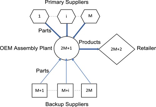
A supply chain with dual suppliers is considered, where one type of product is assembled at OEM plant, using M different part types provided by M primary and M backup suppliers, one primary and one backup supplier for each part type (for notation used, see Table 1).

Table 1. Notation.

Indices
i	=	supply chain node (e.g. supplier, assembly plant, retailer), $i\in I$
k	=	geographic region, $k\in K$
s	=	disruption scenario, $s\in S$
t	=	planning period, $t\in T$
Input parameters
$a_i$	=	fixed cost of reserve capacity for primary supplier, $i\le M$, or OEM plant, i = m, per unit of reserve free capacity
$b_i$	=	variable cost of reserve capacity for primary supplier, $i\le M$, or OEM plant, i = m, per unit of deployed capacity
${\alpha }_i$	=	fixed cost per part of pre-positioning RMI of part type $i\le M$ at OEM plant
${\text{β}}_i$	=	variable cost per part of usage RMI of part type $i\le M$ pre-positioned at OEM plant
$c_i$	=	nominal per period capacity of supplier, $i\le 2M$, or OEM plant i = m
${\tilde{d}}_t$	=	original market demand in period t
$d_t^s$	=	market demand in period t, under disruption scenario s
$e_i$	=	per unit price of parts purchased from supplier $i\in I:i\le 2M$
$f_i$	=	fixed ordering cost for backup supplier, $i\in I:M+1\le i\le 2M$
γ	=	per unit penalty cost of unfulfilled demand for products
$p_k$	=	probability of regional disruption for region k
${\delta }_{it}^s$	=	zero-one availability coefficient for supplier, $i\le 2M$, or OEM plant i = m, in period, $t\in T$, under disruption scenario, $s\in S$
${\sigma }_i$	=	manufacturing and transportation time from supplier i to OEM plant
${\tau }_i^s$	=	delivery lead time from supplier i to OEM plant under disruption scenario s
${\theta }_k$	=	duration of regional disruption in region, $k\in K$
${\vartheta }_k$	=	delay time for the ripple effect in region, $k\in K:k>1$

The supply chain consists of 2M + 2 supply chain nodes (see Figure 1) $i\in I=\{1,\dots ,M,M+1,\dots ,2M,2M+1,2M+2\},$dispersed across n geographic regions, $k\in K=\{1,\dots ,n\}$. There are M primary suppliers, $i\in \{1,\dots ,M\}$, and M backup suppliers, $i\in I=\{M+1,\dots ,2M\}$, one OEM assembly plant, i = 2M + 1, and one retailer, i = 2M + 2. Each part type $i=1,\dots M$, manufactured and supplied by primary supplier, $i\in \{1,\dots ,M\}$ can also be manufactured and supplied by a backup supplier, M + i. Denote by m = 2M + 1, total number of supply chain manufacturing facilities.

Figure 1. Supply chain.

Let $I^k$, be the subset of supply chain nodes in region $k\in K$ and denote by, k = 1, the disruption source region, where the regional pandemic type disruption originates with probability, $p_1$. The disruption in region, k = 1, is propagated across the supply chain and the ripple effect triggers regional disruptions in different regions, $k\in K:k>1$, with probability, $p_k$.

In the supply chain, the ‘all-or-nothing’ type of regional disruption scenarios are considered, which are typical for a pandemic crisis, (e.g. the region unaffected by pandemic crisis or under full lockdown), and hence their total number is, $n^2$. Each scenario $s\in S=\{1,\dots ,n^2\}$ is modelled by 0–1 vector ${\lambda }^s=\{{\lambda }_{1s},\dots ,{\lambda }_{ns}\}$, where ${\lambda }_{ks}\in \{0,1\}$. ${\lambda }_{ks}=1$, if region $k\in K$ is disrupted under scenario $s\in S$; otherwise ${\lambda }_{ks}=0$.

We assume that different geographic regions can be disrupted only by the ripple effect directly propagated from region, k = 1. Under the above assumption, the probability, $P_s$, for each disruption scenario, $s\in S$, can be expressed as follows: (1) $P_s=\{\begin{array}{ll}{\displaystyle \sum _{\overline{s}\in S:{\lambda }_{1\overline{s}}=0}{R}_{\overline{s}},}& {\displaystyle \text{if}\sum _{k\in K}{\lambda }_{ks}=0}\\ 0,& {\displaystyle \text{if}{\lambda }_{1s}=0\text{and}}\\ & {\displaystyle \sum _{k\in K:k>1}{\lambda }_{ks}>0}\\ R_s,\text{otherwise,}\end{array}$(1) where (2) $R_s=\left(\prod _{k\in K:{\lambda }_{ks}=1}{p}_k\right)\left(\prod _{k\in K:{\lambda }_{ks}=0}\right(1-p_k\left)\right);s\in S,$(2) is the binomial probability for the ‘all-or-nothing’ disruption scenario, $s\in S$.

Notice that scenarios with non-disrupted source region, k = 1, and disrupted at least one of the remaining regions are infeasible and hence their probabilities are zero. Simultaneously, the probability of scenarios with all regions non-disrupted, (i.e. ${\lambda }_{ks}=0\mathrm{\forall }k\in K$), is, $\sum _{s\in S:{\lambda }_{1s}=0}{R}_s$.

The disruption in region, k = 1, starts at the beginning of the horizon and the supply chain operations are considered over a finite planning horizon, $T=\{1,\dots ,h\}$. Let ${\vartheta }_k;k\in K:k>1$, be the delay time of the ripple effect for region, $k\in K:k>1$, i.e. the ripple effect in region, k>1, is observed, ${\vartheta }_k$, periods after the outbreak of disruption in region, k = 1. Denote by ${\theta }_k$, the duration of regional disruption in region $k\in K$, so that the disruption in region k>1, ends, ${\vartheta }_k+{\theta }_k$, periods after the disruption start in region, k = 1.

The disruptions imply extended delivery lead times. Let ${\tau }_i^s$ be the delivery lead time from supplier, $i\in I^k:i\le 2M$, in region k to OEM plant, under disruption scenario s. ${\tau }_i^s$, includes manufacturing and transportation time from supplier i to OEM plant, ${\sigma }_i$, and duration of regional disruption, ${\theta }_k$ (3) ${\tau }_i^s={\sigma }_i+{\theta }_k{\lambda }_{ks};i\in I^k,k\in K,s\in S:i\le 2M.$(3) Denote by ${\tilde{d}}_t$, the original market demand for products in period $t\in T$. Thus the total market demand is $\tilde{D}=\sum _{t\in T}{\tilde{d}}_t$. Since the ripple effect may cause simultaneous supply and demand disruptions, the original demand may randomly change. For each disruption scenario s, denote by $d_t^s$ and $D_t^s=\sum _{t^{\prime }\in T:t^{\prime }\le t}{d}_{t^{\prime }}^s$, demand in period t and cumulative demand by period t, respectively.

To simplify the problem presentation, we assume that demand for each part type is identical with demand for products, i.e. one unit of each part type is needed for one unit of product. If the total demand for products cannot be fulfilled during the planning horizon, the manufacturer can be charged with penalty cost for unfulfilled demand, γ, per unit.

For each supplier of parts $i\in I:i\le 2M$ and each disruption scenario $s\in S$, define the order fulfilment coefficient, (4) $g_i^s=(h-{\theta }_k{\lambda }_{ks})/h;i\in I^k,k\in K,s\in S:i\le 2M$(4) The coefficient, $g_i^s$, represents the fraction of total demand for parts delivered to OEM plant by supplier, $i\in I^k:i\le 2M$, in region k under disruption scenario s.

In addition, denote by ${\delta }_{it}^s\in \{0,1\}$, the availability coefficient for capacity of each facility. ${\delta }_{it}^s$ is defined for each supplier ($i\le 2M$), and OEM plant (i = 2M + 1), each period, $t\in T$, and all regional disruption scenarios for $k\in K$, where $i\in I^k$. (5) ${\delta }_{it}^s=\{\begin{array}{ll}0& \text{if}{\lambda }_{ks}=1\text{and}\\ & t\in T_{ks},\\ 1& \text{otherwise},\end{array}i\in I^k,k\in K,s\in S,t\in T$(5) where $T_{ks}$ is the subset of lockdown periods for region k and scenario s.

4. Supply chain viability model

In this section, stochastic quadratic MIP (Mixed Integer Programming) model Viabil_WD is developed to maintain viability of a supply chain under the ripple effect caused by propagated regional disruption risks. The supply chain viability can be maintained by recovery backup supplies of parts to OEM assembly plant, capacity reservation at primary suppliers and OEM assembly plant and pre-positioning RMI of parts at OEM plant.

Let $E^c$, (6(6) $\begin{array}{rl}{E}^c& =\sum _{s\in S}\sum _{i\in I:M+1\le i\le 2M}{P}_s{f}_i{u}_i^s/\tilde{D}\\ & +\sum _{s\in S}{P}_s(\sum _{i\in I:i\le M}{e}_i{g}_i^s+\sum _{i\in I:M+1\le i\le 2M}{e}_i{v}_i^s)\\ & +\sum _{i=1,\dots ,M,2M+1}(a_i{q}_i+\sum _{s\in S}{P}_s{b}_i{r}_i^s)/\tilde{D}\\ & +\sum _{i\in I:i\le M}({\alpha }_i{y}_i+\sum _{s\in S}{P}_s{\text{β}}_i{z}_i^s)/\tilde{D}\\ & +\gamma \sum _{s\in S}{P}_s(D_h^s-\sum _{t\in T}{x}_{mt}^s)/\tilde{D}.\end{array}$(6) ), be the minimised expected cost per product, and $E^{sl}$, (7(7) $\begin{array}{rl}{E}^{sl}& =\frac{\sum _{t\in T}\sum _{s\in S}{P}_s{x}_{mt}^s}{\sum _{s\in S}{P}_s{D}_h^s}.\end{array}$(7) ), the maximised expected service level (i.e. the expected fraction of fulfilled demand for products). (6) $\begin{array}{rl}{E}^c& =\sum _{s\in S}\sum _{i\in I:M+1\le i\le 2M}{P}_s{f}_i{u}_i^s/\tilde{D}\\ & +\sum _{s\in S}{P}_s(\sum _{i\in I:i\le M}{e}_i{g}_i^s+\sum _{i\in I:M+1\le i\le 2M}{e}_i{v}_i^s)\\ & +\sum _{i=1,\dots ,M,2M+1}(a_i{q}_i+\sum _{s\in S}{P}_s{b}_i{r}_i^s)/\tilde{D}\\ & +\sum _{i\in I:i\le M}({\alpha }_i{y}_i+\sum _{s\in S}{P}_s{\text{β}}_i{z}_i^s)/\tilde{D}\\ & +\gamma \sum _{s\in S}{P}_s(D_h^s-\sum _{t\in T}{x}_{mt}^s)/\tilde{D}.\end{array}$(6) (7) $\begin{array}{rl}{E}^{sl}& =\frac{\sum _{t\in T}\sum _{s\in S}{P}_s{x}_{mt}^s}{\sum _{s\in S}{P}_s{D}_h^s}.\end{array}$(7) The expected cost, $E^c$, (6(6) $\begin{array}{rl}{E}^c& =\sum _{s\in S}\sum _{i\in I:M+1\le i\le 2M}{P}_s{f}_i{u}_i^s/\tilde{D}\\ & +\sum _{s\in S}{P}_s(\sum _{i\in I:i\le M}{e}_i{g}_i^s+\sum _{i\in I:M+1\le i\le 2M}{e}_i{v}_i^s)\\ & +\sum _{i=1,\dots ,M,2M+1}(a_i{q}_i+\sum _{s\in S}{P}_s{b}_i{r}_i^s)/\tilde{D}\\ & +\sum _{i\in I:i\le M}({\alpha }_i{y}_i+\sum _{s\in S}{P}_s{\text{β}}_i{z}_i^s)/\tilde{D}\\ & +\gamma \sum _{s\in S}{P}_s(D_h^s-\sum _{t\in T}{x}_{mt}^s)/\tilde{D}.\end{array}$(6) ), contains different fixed and variable costs per product.

The fixed cost is the cost of backup contracts, $\sum _{s\in S}\sum _{i\in I:M+1\le i\le 2M}{P}_s{f}_i{u}_i^s/\tilde{D}$.

The variable costs includes cost: of purchasing parts from primary and recovery suppliers, $\sum _{s\in S}{P}_s(\sum _{i\in I:i\le M}{e}_i{g}_i^s+\sum _{i\in I:M+1\le i\le 2M}{e}_i{v}_i^s)$, of pre-positioning and usage of RMI at OEM plant, $\sum _{i\in I:i\le M}({\alpha }_i{y}_i+\sum _{s\in S}{P}_s{\text{β}}_i{z}_i^s)/\tilde{D}$, of capacity reservation and deployment, $\sum _{i=1,\dots ,M,2M+1}(a_i{q}_i+\sum _{s\in S}{P}_s{b}_i{r}_i^s)/\tilde{D}$ and of penalty for unfulfilled demand, $\gamma \sum _{s\in S}{P}_s(D_h^s-\sum _{t\in T}{x}_{mt}^s)/\tilde{D}=\gamma (1-E^{sl})\sum _{s\in S}{P}_s{D}_h^s/\tilde{D}$. Note that the cost and the service level objectives are in conflict (e.g. Sawik 2015). As a consequence, the associated cost- and service-optimal production schedules for OEM assembly plant form boundaries for all acceptable production trajectories. Define by $X_t^s$ and $Y_t^s$, respectively cost-optimal and service-optimal production for OEM assembly plant in period $t\in T$ under disruption scenario $s\in S$. In other words, $X_t^s$ and $Y_t^s$ are the optimal solution value of $x_{mt}^s$, for the problem of minimising expected cost and maximising expected service level, respectively. The objective of model Viabil_WD is to minimise weighted sum of the expected deviations of production schedule from the two conflicting, boundary production schedules: cost-optimal, $X_t^s$ and service-optimal, $Y_t^s$, over the entire planning horizon, $t\in T$, and across all disruption scenarios, $s\in S$. The problem is a multi-portfolio stochastic optimisation in which for each disruption scenario, recovery supply portfolio is selected along with the deployment of capacity reserved at primary suppliers and OEM plant, and the usage of RMI of parts pre-positioned at OEM plant, e.g. Sawik (2017, 2019). The recovery supply portfolio is defined below (for definitions of problem variables, see Table 2).

The recovery supply portfolio for scenario s

(8) $(v_{M+1}^s,\dots ,v_{2M}^s)$(8) represents supplies of parts from M backup suppliers to OEM plant, where (9) $\begin{array}{rl}& v_{M+i}^s\in [0,1];i\in I,s\in S:i\le M\end{array}$(9) (10) $\begin{array}{rl}& g_i^s+v_{M+i}^s=1;i\in I,s\in S:i\le M,\end{array}$(10) where $g_i^s$, Equation (4(4) $g_i^s=(h-{\theta }_k{\lambda }_{ks})/h;i\in I^k,k\in K,s\in S:i\le 2M$(4) ), is the fraction of total demand for parts delivered to OEM plant by primary supplier i under disruption scenario s.

Table 2. Problem variables.

$q_i$	$\ge$	0, reserve capacity production rate at primary supplier, $i\le M$ or OEM plant, i = m, (capacity reservation)
$r_i^s$	$\ge$	0, reserve capacity production rate deployed at primary supplier, $i\le M$ or OEM plant, i = m, under disruption scenario s (reserve capacity deployment)
$u_i^s$	$\in$	$\{0,1\}$, where the value 1 means that backup supplier, $i\in I:M+1\le i\le 2M$, is selected as a recovery supplier under disruption scenario s; otherwise $u_i^s=0$ (recovery supplier selection)
$v_i^s$	$\in$	$[0,1]$, fraction of total demand for parts, ordered from recovery supplier, $M+1\le i\le 2M$, under disruption scenario s (recovery supply portfolio)
$x_{it}^s$	$\ge$	0, production of facility, $i\in I$, in period $t\in T$, under disruption scenario s (production of parts/products)
$y_i$	$\ge$	0, RMI of part type $i\in I:i\le M$, pre-positioned at OEM plant (pre-positioning of RMI)
$z_i^s$	$\ge$	0, RMI of part type $i\in I:i\le M$, pre-positioned at OEM plant and used under disruption scenario s (usage of RMI)
Auxiliary variable
$w_t^s$	$\in$	$\mathrm{\Re }$, inventory (if $w_t^s\ge 0$) or shortage (if $w_t^s<0$) of products at OEM plant at the beginning of period $t\in T\bigcup \{h+1\}$ under disruption scenario s (finished product inventory)

Model Viabil_WD is a deterministic equivalent of the two-stage stochastic program with recourse, e.g. Sawik (2020). The capacity reservation and RMI pre-positioning variables, $q_i,y_i$, are referred to as first-stage decisions, and the scenario-dependent reserve capacity deployment and RMI usage variables, $r_i^s,z_i^s$, recovery supply portfolio selection variables, $u_i^s,v_i^s$, and production and inventory scheduling variables, $x_{it}^s,w_t^s$, are referred to as recourse or second-stage decisions (cf. Table 2).

Since the objectives (6(6) $\begin{array}{rl}{E}^c& =\sum _{s\in S}\sum _{i\in I:M+1\le i\le 2M}{P}_s{f}_i{u}_i^s/\tilde{D}\\ & +\sum _{s\in S}{P}_s(\sum _{i\in I:i\le M}{e}_i{g}_i^s+\sum _{i\in I:M+1\le i\le 2M}{e}_i{v}_i^s)\\ & +\sum _{i=1,\dots ,M,2M+1}(a_i{q}_i+\sum _{s\in S}{P}_s{b}_i{r}_i^s)/\tilde{D}\\ & +\sum _{i\in I:i\le M}({\alpha }_i{y}_i+\sum _{s\in S}{P}_s{\text{β}}_i{z}_i^s)/\tilde{D}\\ & +\gamma \sum _{s\in S}{P}_s(D_h^s-\sum _{t\in T}{x}_{mt}^s)/\tilde{D}.\end{array}$(6) ) and (7(7) $\begin{array}{rl}{E}^{sl}& =\frac{\sum _{t\in T}\sum _{s\in S}{P}_s{x}_{mt}^s}{\sum _{s\in S}{P}_s{D}_h^s}.\end{array}$(7) ) are in conflict, the cost-optimal production schedule, $X_t^s,t\in T$, is simultaneously the worst schedule with respect to customer service, and vice versa, $Y_t^s,t\in T$, which is service-optimal is worst with respect to expected cost. 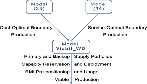Thus the two extreme production schedules, $X_t^s,t\in T$ and $Y_t^s,t\in T$, define acceptable boundaries for any production trajectory, for a given disruption scenario s and a given portfolio of implementable decisions. As a consequence, the supply chain viability can be implicitly maintained under the ripple effect by solving the following stochastic quadratic optimisation problem (see Figure 2). Viabil_WD: Maintaining of supply chain Viability by minimising Weighted Deviations from cost-optimal and service-optimal production schedules

Figure 2. Maintaining of supply chain viability.

Minimise (11) $\lambda \sum _{t\in T}\sum _{s\in S}{P}_s(x_{mt}^s-X_t^s{)}^2+(1-\lambda \left)\sum _{t\in T}\sum _{s\in S}{P}_s\right(x_{mt}^s-Y_t^s{)}^2$(11) where $0\le \lambda \le 1$ is the weight factor subject to (6(6) $\begin{array}{rl}{E}^c& =\sum _{s\in S}\sum _{i\in I:M+1\le i\le 2M}{P}_s{f}_i{u}_i^s/\tilde{D}\\ & +\sum _{s\in S}{P}_s(\sum _{i\in I:i\le M}{e}_i{g}_i^s+\sum _{i\in I:M+1\le i\le 2M}{e}_i{v}_i^s)\\ & +\sum _{i=1,\dots ,M,2M+1}(a_i{q}_i+\sum _{s\in S}{P}_s{b}_i{r}_i^s)/\tilde{D}\\ & +\sum _{i\in I:i\le M}({\alpha }_i{y}_i+\sum _{s\in S}{P}_s{\text{β}}_i{z}_i^s)/\tilde{D}\\ & +\gamma \sum _{s\in S}{P}_s(D_h^s-\sum _{t\in T}{x}_{mt}^s)/\tilde{D}.\end{array}$(6) ), (7(7) $\begin{array}{rl}{E}^{sl}& =\frac{\sum _{t\in T}\sum _{s\in S}{P}_s{x}_{mt}^s}{\sum _{s\in S}{P}_s{D}_h^s}.\end{array}$(7) ) and

Recovery supplier selection constraints (12) $\begin{array}{rl}& v_i^s\le u_i^s;i\in I,s\in S:M+1<i\le 2M\end{array}$(12) (13) $\begin{array}{rl}& g_i^s+v_{M+i}^s=1;i\in I,s\in S:i\le M\end{array}$(13) Capacity reservation constraints (14) $\begin{array}{rl}& q_i\le {\phi }_i{c}_i;i\in I:i\le M\text{or}i=m\end{array}$(14) (15) $\begin{array}{rl}& r_i^s\le q_i;i\in I,s\in S:i\le M\text{or}i=m,\end{array}$(15) where ${\phi }_i\in (0,1]$.

Production constraints (16) $\begin{array}{rl}& \sum _{t\in T}{x}_{it}^s/\tilde{D}\le g_i^s;i\in I,s\in S:i\le M\end{array}$(16) (17) $\begin{array}{rl}& \sum _{t\in T}{x}_{it}^s/\tilde{D}\le v_i^s;i\in I,s\in S:M+1\le i\le 2M\end{array}$(17) (18) $\begin{array}{rl}& x_{it}^s\le {\delta }_{it}^s(c_i+r_i^s);i\in I,t\in T,s\in S:i\le m,\end{array}$(18) where $r_i^s=0$ for backup suppliers, $M+1\le i\le 2M$.

RMI constraints (19) $\begin{array}{rl}& y_i\le {\overline{\tau }}_{M+i}{c}_m;i\in I:i\le M\end{array}$(19) (20) $\begin{array}{rl}& z_i^s\le y_i;i\in I,s\in S:i\le M,\end{array}$(20) where ${\overline{\tau }}_{M+i}=\sum _{s\in S}{P}_s{\tau }_{M+i}^s$ is the expected delivery lead time for backup supplier, M + i.

Suppliers-manufacturer coordinating constraints: (21) $\begin{array}{rl}& \sum _{t^{\prime }\in T:t^{\prime }\le t}{x}_{m{t}^{\prime }}^s\le \sum _{t^{\prime }\in T:t^{\prime }\le t-{\tau }_i^s}{x}_{i{t}^{\prime }}^s+\sum _{t^{\prime }\in T:t^{\prime }\le t-{\tau }_{M+i}^s}{x}_{M+i,t^{\prime }}^s\\ & +z_i^s;i\in I,t\in T,s\in S:i\le M\end{array}$(21) Inventory constraints: (22) $\begin{array}{rl}& w_{t+1}^s=w_t^s+x_{mt}^s-d_t^s;t\in T,s\in S\end{array}$(22) (23) $\begin{array}{rl}& w_1^s=0;s\in S\end{array}$(23) Bounds on maximum expected cost and minimum expected service level (24) $\begin{array}{rl}& E^c\le ({\underset{\_}{E}}^c+{\overline{E}}^c)/2\end{array}$(24) (25) $\begin{array}{rl}& E^{sl}\ge ({\underset{\_}{E}}^{sl}+{\overline{E}}^{sl})/2,\end{array}$(25) where ${\underset{\_}{E}}^c,{\overline{E}}^c$ and ${\underset{\_}{E}}^{sl},{\overline{E}}^{sl}$, are the minimum and maximum values of expected cost and expected service level (see Section 3.1), respectively.

Non-negativity and integrality conditions: (26) $\begin{array}{rl}& q_i\ge 0;i\in I:i\le M\text{or}i=m\end{array}$(26) (27) $\begin{array}{rl}& r_i^s\ge 0;i\in I,s\in S:i\le M\text{or}i=m\end{array}$(27) (28) $\begin{array}{rl}& u_i^s\in \{0,1\};i\in I,s\in S:M+1\le i\le 2M\end{array}$(28) (29) $\begin{array}{rl}& v_i^s\in [0,1];i\in I,s\in S:M+1\le i\le 2M\end{array}$(29) (30) $\begin{array}{rl}& x_{it}^s\ge 0;i\in I,t\in T,s\in S:i\le m\end{array}$(30) (31) $\begin{array}{rl}& y_i\ge 0;i\in I:i\le M\end{array}$(31) (32) $\begin{array}{rl}& z_i^s\ge 0;i\in I,s\in S:i\le M\end{array}$(32) where $T^{\ast }=T\bigcup \{h+1\}=\{1,\dots ,h,h+1\}$, and h + 1, is a dummy period.

Equation (12(12) $\begin{array}{rl}& v_i^s\le u_i^s;i\in I,s\in S:M+1<i\le 2M\end{array}$(12) ) ensures against assignment of the recovery supplies to non-selected backup suppliers. Equation (13(13) $\begin{array}{rl}& g_i^s+v_{M+i}^s=1;i\in I,s\in S:i\le M\end{array}$(13) ) guarantees that for each part type, i, the unfulfilled demand, ($1-g_i^s$), is met by recovery supplies.

The capacity reservation constraint (14(14) $\begin{array}{rl}& q_i\le {\phi }_i{c}_i;i\in I:i\le M\text{or}i=m\end{array}$(14) ) ensures that reserve capacity production rate of primary suppliers of parts and of OEM plant cannot exceed given fractions, ${\phi }_i$, of their full per period capacity, and Equation (15(15) $\begin{array}{rl}& r_i^s\le q_i;i\in I,s\in S:i\le M\text{or}i=m,\end{array}$(15) ) limits the reserve capacity deployment by the reserve capacity production rate.

The production constraints (16(16) $\begin{array}{rl}& \sum _{t\in T}{x}_{it}^s/\tilde{D}\le g_i^s;i\in I,s\in S:i\le M\end{array}$(16) ) and (17(17) $\begin{array}{rl}& \sum _{t\in T}{x}_{it}^s/\tilde{D}\le v_i^s;i\in I,s\in S:M+1\le i\le 2M\end{array}$(17) ) guarantee that the total production of each part type by primary and recovery suppliers is limited by the primary and recovery supply portfolios, respectively. In addition, the capacity constraint (18(18) $\begin{array}{rl}& x_{it}^s\le {\delta }_{it}^s(c_i+r_i^s);i\in I,t\in T,s\in S:i\le m,\end{array}$(18) ) ensures that in every period, production of each part type and finished products is bounded by available capacity, enlarged by deployed reserve capacity for primary suppliers and OEM plant.

Equation (19(19) $\begin{array}{rl}& y_i\le {\overline{\tau }}_{M+i}{c}_m;i\in I:i\le M\end{array}$(19) ) ensures for each part type that the RMI pre-positioned at OEM plant does not exceed the plant per period capacity during the average lead time from the backup suppliers, and, in addition, the usage of RMI is limited by Equation (20(20) $\begin{array}{rl}& z_i^s\le y_i;i\in I,s\in S:i\le M,\end{array}$(20) ).

Equation (21(21) $\begin{array}{rl}& \sum _{t^{\prime }\in T:t^{\prime }\le t}{x}_{m{t}^{\prime }}^s\le \sum _{t^{\prime }\in T:t^{\prime }\le t-{\tau }_i^s}{x}_{i{t}^{\prime }}^s+\sum _{t^{\prime }\in T:t^{\prime }\le t-{\tau }_{M+i}^s}{x}_{M+i,t^{\prime }}^s\\ & +z_i^s;i\in I,t\in T,s\in S:i\le M\end{array}$(21) ) ensures that cumulative production at OEM plant is not exceeding cumulative production of each part type at primary and recovery suppliers plus the usage of RMI.

The auxiliary constraints (22(22) $\begin{array}{rl}& w_{t+1}^s=w_t^s+x_{mt}^s-d_t^s;t\in T,s\in S\end{array}$(22) )–(23(23) $\begin{array}{rl}& w_1^s=0;s\in S\end{array}$(23) ) determine the inventory (or shortage) of products at OEM plant at the beginning of each period, $t\in T^{\ast }$.

The quadratic objective function (11(11) $\lambda \sum _{t\in T}\sum _{s\in S}{P}_s(x_{mt}^s-X_t^s{)}^2+(1-\lambda \left)\sum _{t\in T}\sum _{s\in S}{P}_s\right(x_{mt}^s-Y_t^s{)}^2$(11) ) defines the weighted sum deviation of the expected production schedule from the two extreme, boundary production schedules, $X_t^s,t\in T$, and $Y_t^s,t\in T$, associated with the two conflicting objectives (6(6) $\begin{array}{rl}{E}^c& =\sum _{s\in S}\sum _{i\in I:M+1\le i\le 2M}{P}_s{f}_i{u}_i^s/\tilde{D}\\ & +\sum _{s\in S}{P}_s(\sum _{i\in I:i\le M}{e}_i{g}_i^s+\sum _{i\in I:M+1\le i\le 2M}{e}_i{v}_i^s)\\ & +\sum _{i=1,\dots ,M,2M+1}(a_i{q}_i+\sum _{s\in S}{P}_s{b}_i{r}_i^s)/\tilde{D}\\ & +\sum _{i\in I:i\le M}({\alpha }_i{y}_i+\sum _{s\in S}{P}_s{\text{β}}_i{z}_i^s)/\tilde{D}\\ & +\gamma \sum _{s\in S}{P}_s(D_h^s-\sum _{t\in T}{x}_{mt}^s)/\tilde{D}.\end{array}$(6) ) and (7(7) $\begin{array}{rl}{E}^{sl}& =\frac{\sum _{t\in T}\sum _{s\in S}{P}_s{x}_{mt}^s}{\sum _{s\in S}{P}_s{D}_h^s}.\end{array}$(7) ), respectively. In addition, constraints (24(24) $\begin{array}{rl}& E^c\le ({\underset{\_}{E}}^c+{\overline{E}}^c)/2\end{array}$(24) ) and (25(25) $\begin{array}{rl}& E^{sl}\ge ({\underset{\_}{E}}^{sl}+{\overline{E}}^{sl})/2,\end{array}$(25) ) impose upper and lower bound, respectively on expected cost and expected service level. Thus the optimal solution of Viabil_WD aims at keeping the production trajectory within the acceptable boundaries implied by the two conflicting objectives and hence maintains the supply chain viability under the ripple effect. At the same time, constraints (24(24) $\begin{array}{rl}& E^c\le ({\underset{\_}{E}}^c+{\overline{E}}^c)/2\end{array}$(24) ) and (25(25) $\begin{array}{rl}& E^{sl}\ge ({\underset{\_}{E}}^{sl}+{\overline{E}}^{sl})/2,\end{array}$(25) ) ensure the two conflicting objectives against their deterioration.

Boundaries for production trajectory

The minimum and maximum values of the two objective functions, $E^c$, (6(6) $\begin{array}{rl}{E}^c& =\sum _{s\in S}\sum _{i\in I:M+1\le i\le 2M}{P}_s{f}_i{u}_i^s/\tilde{D}\\ & +\sum _{s\in S}{P}_s(\sum _{i\in I:i\le M}{e}_i{g}_i^s+\sum _{i\in I:M+1\le i\le 2M}{e}_i{v}_i^s)\\ & +\sum _{i=1,\dots ,M,2M+1}(a_i{q}_i+\sum _{s\in S}{P}_s{b}_i{r}_i^s)/\tilde{D}\\ & +\sum _{i\in I:i\le M}({\alpha }_i{y}_i+\sum _{s\in S}{P}_s{\text{β}}_i{z}_i^s)/\tilde{D}\\ & +\gamma \sum _{s\in S}{P}_s(D_h^s-\sum _{t\in T}{x}_{mt}^s)/\tilde{D}.\end{array}$(6) ) and $E^{sl}$, (7(7) $\begin{array}{rl}{E}^{sl}& =\frac{\sum _{t\in T}\sum _{s\in S}{P}_s{x}_{mt}^s}{\sum _{s\in S}{P}_s{D}_h^s}.\end{array}$(7) ) are calculated below.

The minimum and maximum values of expected cost ${\underset{\_}{E}}^c,{\overline{E}}^c$, and expected service level, ${\underset{\_}{E}}^{sl},{\overline{E}}^{sl}$, are solutions of the following stochastic MIP problems: (33) $\begin{array}{rl}& min\left\{\left(6\right)\text{s.t. (12)--(21), (26)--(32)}\right\}\end{array}$(33) (34) $\begin{array}{rl}& max\left\{\left(7\right)\text{s.t. (12)--(21), (26)--(32)}\right\}\end{array}$(34) In (33(33) $\begin{array}{rl}& min\left\{\left(6\right)\text{s.t. (12)--(21), (26)--(32)}\right\}\end{array}$(33) ), $E^c$ is the minimised objective function, while $E^{sl}$ is not considered, whereas in (34(34) $\begin{array}{rl}& max\left\{\left(7\right)\text{s.t. (12)--(21), (26)--(32)}\right\}\end{array}$(34) ), $E^{sl}$ is the maximised objective function, while $E^c$ is not considered. Thus solution of (33(33) $\begin{array}{rl}& min\left\{\left(6\right)\text{s.t. (12)--(21), (26)--(32)}\right\}\end{array}$(33) ) yields the minimum value ${\underset{\_}{E}}^c$ of $E^c$ and the minimum value ${\underset{\_}{E}}^{sl}$ of $E^{sl}$, whereas solution of (34(34) $\begin{array}{rl}& max\left\{\left(7\right)\text{s.t. (12)--(21), (26)--(32)}\right\}\end{array}$(34) ) yields the maximum value ${\overline{E}}^{sl}$ of $E^{sl}$ and the maximum value ${\overline{E}}^c$ of $E^c$. Simultaneously, the associated cost- and service-optimal production schedules, ($x_{mt}^s,t\in T$), for OEM assembly plant are determined, respectively $X_t^s,t\in T$, and $Y_t^s,t\in T$, to establish boundaries for all acceptable production trajectories.

In the viability theory, the width of the viability kernel represents the degree of system resilience. In a similar way, the degree of supply chain resilience can be measured by the distance between cost- and service-optimal boundary production trajectories. For example, by the minimum expected distance over a planning horizon (35) $\underset{t\in T}{min}\sum _{s\in S}{P}_s|X_t^s-Y_t^s|.$(35) The greater the minimum distance (35(35) $\underset{t\in T}{min}\sum _{s\in S}{P}_s|X_t^s-Y_t^s|.$(35) ), the higher the supply chain resilience to the ripple effect. Since the boundary trajectories are associated with the optimal solutions of (33(33) $\begin{array}{rl}& min\left\{\left(6\right)\text{s.t. (12)--(21), (26)--(32)}\right\}\end{array}$(33) ) and (34(34) $\begin{array}{rl}& max\left\{\left(7\right)\text{s.t. 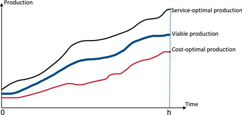(12)--(21), (26)--(32)}\right\}\end{array}$(34) ), the minimum distance (35(35) $\underset{t\in T}{min}\sum _{s\in S}{P}_s|X_t^s-Y_t^s|.$(35) ) can be extended and by that the supply chain resilience improved only by relaxing bounds on available controls, e.g. by allowing for greater reservation capacities, higher levels of RMI or by selecting more efficient and reliable primary and backup suppliers. Figure 3 illustrates the concept of a viable production trajectory, which is located between the two curvilinear boundary trajectories: cost-optimal and service-optimal. The region between the two boundaries represents the supply chain viable production states. The regions above the service-optimal trajectory and below the cost-optimal trajectory represent production states that may yield the costs higher than the highest possible cost and the service levels lower than the lowest possible service level, respectively, Thus a single objective optimisation of supply chain operations with respect to the expected cost (33(33) $\begin{array}{rl}& min\left\{\left(6\right)\text{s.t. (12)--(21), (26)--(32)}\right\}\end{array}$(33) ) or to the expected service level (34(34) $\begin{array}{rl}& max\left\{\left(7\right)\text{s.t. (12)--(21), (26)--(32)}\right\}\end{array}$(34) ) only, which pushes production to boundaries of a viability region is not recommended under severe disruption risks. Then a more severe disruption may push the production outside the viability region and cause greater losses.

Figure 3. Boundary production trajectories.

Notice that the mathematical formulation proposed for supply chain viability can also be applied to directly improve supply chain resilience, by optimising the trade-off between cost and service, for example by minimising weighted sum of normalised expected cost and expected service level. Such a resilient solution can be obtained by solving the following, stochastic linear mixed integer program. Resil_WS: Improving supply chain Resilience by minimising Weighted Sum of normalised expected cost and service level

Minimise (36) $\lambda \frac{E^c-{\underset{\_}{E}}^c}{{\overline{E}}^c-{\underset{\_}{E}}^c}+(1-\lambda )\frac{{\overline{E}}^{sl}-E^{sl}}{{\overline{E}}^{sl}-{\underset{\_}{E}}^{sl}}$(36) subject to (6(6) $\begin{array}{rl}{E}^c& =\sum _{s\in S}\sum _{i\in I:M+1\le i\le 2M}{P}_s{f}_i{u}_i^s/\tilde{D}\\ & +\sum _{s\in S}{P}_s(\sum _{i\in I:i\le M}{e}_i{g}_i^s+\sum _{i\in I:M+1\le i\le 2M}{e}_i{v}_i^s)\\ & +\sum _{i=1,\dots ,M,2M+1}(a_i{q}_i+\sum _{s\in S}{P}_s{b}_i{r}_i^s)/\tilde{D}\\ & +\sum _{i\in I:i\le M}({\alpha }_i{y}_i+\sum _{s\in S}{P}_s{\text{β}}_i{z}_i^s)/\tilde{D}\\ & +\gamma \sum _{s\in S}{P}_s(D_h^s-\sum _{t\in T}{x}_{mt}^s)/\tilde{D}.\end{array}$(6) )–(7(7) $\begin{array}{rl}{E}^{sl}& =\frac{\sum _{t\in T}\sum _{s\in S}{P}_s{x}_{mt}^s}{\sum _{s\in S}{P}_s{D}_h^s}.\end{array}$(7) ), (12(12) $\begin{array}{rl}& v_i^s\le u_i^s;i\in I,s\in S:M+1<i\le 2M\end{array}$(12) )–(32(32) $\begin{array}{rl}& z_i^s\ge 0;i\in I,s\in S:i\le M\end{array}$(32) ), where the values of the minimised objective functions in (36(36) $\lambda \frac{E^c-{\underset{\_}{E}}^c}{{\overline{E}}^c-{\underset{\_}{E}}^c}+(1-\lambda )\frac{{\overline{E}}^{sl}-E^{sl}}{{\overline{E}}^{sl}-{\underset{\_}{E}}^{sl}}$(36) ) are scaled into the interval [0,1], and $0\le \lambda \le 1$ is the weight factor.

5. Computational examples

The basic input data for the computational examples presented in this section are associated with a real-world supply chain in smartphone manufacturing industry. They are based in part on the case study described in Kim and Chung (2022). The supply chain considered consists of 11 supply chain nodes (primary and backup suppliers of parts and OEM assembly plant) plus one domestic retailer, all dispersed across six geographic regions. The input parameters are presented below and in Table 3.

Table 3. Input parameters.

$m=11,I=\{1,\dots ,m,m+1\}$, 12 supply chain nodes (10 suppliers, one manufacturer and one retailer of finished products)
M = 5 primary suppliers, $i=1,\dots ,M$; M = 5 backup suppliers, $i=M+1,\dots ,2M$; assembly plant, i = m, retailer, i = m + 1
i = 1, 6 non-semiconductor suppliers, i = 2, 7 semiconductor foundry, i = 3, 8 semiconductor memory suppliers,
i = 4, 9 display suppliers, i = 5, 10 battery suppliers, i = 11 OEM assembly plant, i = 12 domestic retailer
$n=6,K=\{1,\dots ,n\}$, $2^n=64$	six geographic regions, 64 disruption scenarios
k = 1 China, k = 2 Taiwan, k = 3 Japan, k = 4 Korea, k = 5 EU, k = 6 USA
$I^1=\{1,11\},I^2=\{2,3\},I^3=\{4,5\},I^4=\{6,7\},I^5=\{8,9,10\},I^6=\left\{12\right\}$
$T=\{1,\dots ,12\}$, h = 12	12 planning periods (months)
${\tilde{d}}_t=1000$ $\mathrm{\forall }t\in T$	original demand per period for parts/products
$\tilde{D}=12000$	total original demand for parts/products
Regional disruption probabilities:
$p_1\in [0.65,0.55],p_2\in [0.55,0.45],p_3\in [0.55,0.45],p_4\in [0.45,0.35],p_5\in [0.30,0.20],p_6\in [0.30,0.20]$
$g_k=(h-{\theta }_k)/h;k\in K:k\le 2M$	yield rate of suppliers in region k
$c_i=\tilde{D},i=1,\dots ,M,c_i=0.75\tilde{D},i=M+1,\dots ,2M,c_m=1.2\tilde{D}$	nominal per period capacity of suppliers and OEM plant
${\phi }_i=0.25$	coefficient of reservation capacity
Cost parameters:
$a_i=0.5\gamma ,i\le M,i=m$, fixed cost of reserve capacity for facility i, per unit of reserving free capacity
$b_i=0.1\gamma ,i\le M,i=m$, variable cost of reserve capacity for facility i, per unit of deployed reserve capacity)
$e_i=\lceil \left(Uniform\right(6,10)\rceil ,i\le M$, $e_i=\lceil \left(Uniform\right(16,20)\rceil ,M+1\le i\le 2M$, price per part for primary and backup suppliers
$f_i=500\lceil \left(Uniform\right(16,20)\rceil$, fixed ordering cost for backup supplier, $M+1\le i\le 2M$
${\alpha }_i=1.5e_i,i\le M$, fixed cost per part of pre-positioning RMI of part type i at OEM plant
${\text{β}}_i=\lceil e_i/4\rceil ,i\le M$, variable cost per part of usage RMI of part type i at OEM plant
$\gamma =60$, per unit penalty cost of unfulfilled demand for products

• Duration of disruption in region, $k\in K$: $\begin{array}{r}{\theta }_k=\{\begin{array}{ll}6,& \text{if}k\in \left\{1\right\}\\ 4,& \text{if}k\in \{2,3,4\}\\ 2,& \text{if}k\in \{5,6\}\end{array}\end{array}$

• Delay time for the ripple effect in region, $k\in K:k>1$: $\begin{array}{r}{\vartheta }_k=\{\begin{array}{ll}1,& \text{if}k=2,3,4\\ 2,& \text{if}k=5,6\end{array}\end{array}$

• Regional lockdown schedules: $\begin{array}{r}{\mathrm{\Delta }}_{kt}^s=\{\begin{array}{ll}0,& \text{if}k=1,{\lambda }_{ks}=1,t\in \{1,2,3,4,5,6\}\\ 0,& \text{if}k=2,3,4,{\lambda }_{ks}=1,t\in \{2,3,4,5\}\\ 0,& \text{if}k=5,6,{\lambda }_{ks}=1,t\in \{3,4\}\\ 1,& \text{otherwise}\end{array}\end{array}$

• Availability coefficients for suppliers and OEM plant: ${\delta }_{it}^s=\underset{k\in K:k<n,i\in I^k}{max}\left({\mathrm{\Delta }}_{kt}^s\right);i\in I,s\in S,t\in T:i\le m$

• Manufacturing and transportation time from supplier i: $\begin{array}{r}{\sigma }_i=\{\begin{array}{ll}1,& \text{if}i=1,6\\ 4,& \text{if}i=2,3,7,8\\ 3,& \text{if}i=4,5,9,10\end{array}\end{array}$

• Market demand for domestic region, k = 6 $\begin{array}{r}{d}_t^s=\{\begin{array}{ll}0.75{\tilde{d}}_t,& \text{if}{\lambda }_{6s}=1;t\in \{3,4,5,6\}\\ 1.25{\tilde{d}}_t,& \text{if}{\lambda }_{6s}=1;t\in \{7,8,9,10\}\\ {\tilde{d}}_t,& \text{if}{\lambda }_{6s}=1;t\notin \{3,\dots ,10\}\\ {\tilde{d}}_t,& \text{otherwise.}\end{array}\end{array}$

Computational results for determining boundary production trajectories using stochastic mixed integer programs (33(33) $\begin{array}{rl}& min\left\{\left(6\right)\text{s.t. (12)--(21), (26)--(32)}\right\}\end{array}$(33) ) and (34(34) $\begin{array}{rl}& max\left\{\left(7\right)\text{s.t. (12)--(21), (26)--(32)}\right\}\end{array}$(34) ) are presented in Table 4, and Table 5 shows viable solutions obtained using stochastic quadratic mixed integer program Viabil_WD for a subset of weight factors $\lambda =0,0.25,0.50,0.75,1$. The results presented in Table 5 indicate that for all weight factors, λ, the viable solution produces identical expected cost, $E^c=80.38$, virtually equal to its upper bound (24(24) $\begin{array}{rl}& E^c\le ({\underset{\_}{E}}^c+{\overline{E}}^c)/2\end{array}$(24) ), $({\underset{\_}{E}}^c+{\overline{E}}^c)/2=80.39$, Simultaneously, the expected service level decreases with λ, from the maximum value, ${\overline{E}}^{sl}=93.47\mathrm{\%}$ for $\lambda =0$, to its lower bound (25(25) $\begin{array}{rl}& E^{sl}\ge ({\underset{\_}{E}}^{sl}+{\overline{E}}^{sl})/2,\end{array}$(25) ), $({\underset{\_}{E}}^{sl}+{\overline{E}}^{sl})/2=80.09\mathrm{\%}$, for $\lambda =0.5,0.75,1$. Since the primary and recovery supplies of parts to OEM plant are delayed by around seven periods due to extended delivery lead times, ${\tau }_i^s,i\le 2M$, (3(3) ${\tau }_i^s={\sigma }_i+{\theta }_k{\lambda }_{ks};i\in I^k,k\in K,s\in S:i\le 2M.$(3) ), production at OEM plant (cf. (21(21) $\begin{array}{rl}& \sum _{t^{\prime }\in T:t^{\prime }\le t}{x}_{m{t}^{\prime }}^s\le \sum _{t^{\prime }\in T:t^{\prime }\le t-{\tau }_i^s}{x}_{i{t}^{\prime }}^s+\sum _{t^{\prime }\in T:t^{\prime }\le t-{\tau }_{M+i}^s}{x}_{M+i,t^{\prime }}^s\\ & +z_i^s;i\in I,t\in T,s\in S:i\le M\end{array}$(21) )) sharply increases in period, t = 7.

Table 4. Computing boundary trajectories.

Minimisation of Expected Cost (6(6) $\begin{array}{rl}{E}^c& =\sum _{s\in S}\sum _{i\in I:M+1\le i\le 2M}{P}_s{f}_i{u}_i^s/\tilde{D}\\ & +\sum _{s\in S}{P}_s(\sum _{i\in I:i\le M}{e}_i{g}_i^s+\sum _{i\in I:M+1\le i\le 2M}{e}_i{v}_i^s)\\ & +\sum _{i=1,\dots ,M,2M+1}(a_i{q}_i+\sum _{s\in S}{P}_s{b}_i{r}_i^s)/\tilde{D}\\ & +\sum _{i\in I:i\le M}({\alpha }_i{y}_i+\sum _{s\in S}{P}_s{\text{β}}_i{z}_i^s)/\tilde{D}\\ & +\gamma \sum _{s\in S}{P}_s(D_h^s-\sum _{t\in T}{x}_{mt}^s)/\tilde{D}.\end{array}$(6) ), model (33(33) $\begin{array}{rl}& min\left\{\left(6\right)\text{s.t. (12)--(21), (26)--(32)}\right\}\end{array}$(33) ): 6722 Var., 69 Bin., 8306 Cons. ${}^{\left(\mathrm{a}\right)}$
Minimum Expected Cost (${\underset{\_}{E}}^c$)	73.68
Minimum Expected Service Level (${\underset{\_}{E}}^{sl}$)	66.70%
Expected Primary Supply Portfolio (% of total demand for part type, i) ${}^{\left(\mathrm{b}\right)}$	1(70%), 2(90%), 3(90%), 4(90%), 5(90%)
Expected Recovery Supply Portfolio (% of total demand for part type, i−5) ${}^{\left(\mathrm{c}\right)}$	6(30%), 7(10%), 8(10%), 9(10%), 10(10%)
Expected Boundary Production Schedule (Period: Production Volume) ${}^{\left(\mathrm{d}\right)}$
t = 1:0, t = 2:0, t = 3:0, t = 4:500, t = 5:500, t = 6:500, t = 7:851, t = 8:965, t = 9:1202, t = 10:1088, t = 11:1219, t = 12:1179
Maximisation of Expected Service Level (7(7) $\begin{array}{rl}{E}^{sl}& =\frac{\sum _{t\in T}\sum _{s\in S}{P}_s{x}_{mt}^s}{\sum _{s\in S}{P}_s{D}_h^s}.\end{array}$(7) ), model (34(34) $\begin{array}{rl}& max\left\{\left(7\right)\text{s.t. (12)--(21), (26)--(32)}\right\}\end{array}$(34) ): 6722 Var., 69 Bin., 8306 Cons. ${}^{\left(\mathrm{a}\right)}$
Maximum Expected Service Level (${\overline{E}}^{sl}$)	93.47%
Maximum Expected Cost (${\overline{E}}^c$)	87.11
Expected Primary Supply Portfolio (% of total demand for part type, i) ${}^{\left(\mathrm{b}\right)}$	1(70%), 2(90%), 3(90%), 4(90%), 5(90%)
Expected Recovery Supply Portfolio (% of total demand for part type, i−5) ${}^{\left(\mathrm{c}\right)}$	6(30%), 7(10%), 8(10%), 9(10%), 10(10%)
Expected Boundary Production Schedule (Period: Production Volume) ${}^{\left(\mathrm{d}\right)}$
t = 1:240, t = 2:600, t = 3:600, t = 4:0, t = 5:600, t = 6:600, t = 7:1395, t = 8:1371, t = 9:1465, t = 10:1387, t = 11:1470, t = 12:1489

${}^{\left(\mathrm{a}\right)}$ Var.=total number of variables, Bin.=number of binary variables, Cons.=number of constraints.

${}^{\left(\mathrm{b}\right)}$ $\sum _{s\in S}{P}_s{g}_i^s;i\le M$.

${}^{\left(\mathrm{c}\right)}$ $\sum _{s\in S}{P}_s{v}_{M+i}^s;i\le M$.

${}^{\left(\mathrm{d}\right)}$ $\sum _{s\in S}{P}_s{x}_{mt}^s;t\in T$.

Table 5. Computational results for supply chain viability model Viabil_WD${}^{\left(\mathrm{a}\right)}$.

Weight factor, λ	0	0.25	0.50	0.75	1
Expected Cost ($E^c$)	80.38	80.38	80.38	80.38	80.38
Expected Service Level ($E^{sl}$)	93.47%	86.78%	80.09%	80.09%	80.09%
Expected Primary Supply Portfolio (% of total demand for part type, i) ${}^{\left(\mathrm{b}\right)}$
1(70%), 2(90%), 3(90%), 4(90%), 5(90%)
Expected Recovery Supply Portfolio (% of total demand for part type, i−5) ${}^{\left(\mathrm{c}\right)}$
6(30%), 7(10%), 8(10%), 9(10%), 10(10%)
Expected Viable Production Trajectory ${}^{\left(\mathrm{d}\right)}$
Period	Production	Production	Production	Production	Production
t = 1	240	180	120	98	76
t = 2	600	450	300	188	76
t = 3	600	450	300	188	76
t = 4	0	125	250	413	576
t = 5	600	575	550	563	576
t = 6	600	575	550	563	576
t = 7	1395	1259	1123	1083	1042
t = 8	1371	1270	1168	1163	1157
t = 9	1465	1399	1333	1363	1383
t = 10	1387	1312	1237	1258	1279
t = 11	1470	1407	1345	1378	1411
t = 12	1489	1411	1334	1352	1370

${}^{\left(\mathrm{a}\right)}$ Var.=6722, Bin.=69, Cons.=8306, model has 204 quadratic objective terms

${}^{\left(\mathrm{b}\right)}$ $\sum _{s\in S}{P}_s{g}_i^s;i\le M$.

${}^{\left(\mathrm{c}\right)}$ $\sum _{s\in S}{P}_s{v}_{M+i}^s;i\le M$.

${}^{\left(\mathrm{d}\right)}$ $\sum _{s\in S}{P}_s{x}_{mt}^s;t\in T$.

Note that both expected primary and expected recovery supply portfolios are identical for all models, which are due to the definition of order fulfillment coefficients  (4(4) $g_i^s=(h-{\theta }_k{\lambda }_{ks})/h;i\in I^k,k\in K,s\in S:i\le 2M$(4) ), and the recovery supply portfolio selection constraints, (10(10) $\begin{array}{rl}& g_i^s+v_{M+i}^s=1;i\in I,s\in S:i\le M,\end{array}$(10) ). Nevertheless, the portfolios are different for different disruption scenarios.

The solution results are also illustrated in Figures 4–8. Figure 4 shows boundary, cost-optimal and service-optimal, production trajectories determined by solving mixed integer programs, (33(33) $\begin{array}{rl}& min\left\{\left(6\right)\text{s.t. (12)--(21), (26)--(32)}\right\}\end{array}$(33) ) for minimum expected cost and (34(34) $\begin{array}{rl}& max\left\{\left(7\right)\text{s.t. (12)--(21), (26)--(32)}\right\}\end{array}$(34) ) for maximum expected service level, respectively. In-between the two boundaries, Figure 4 shows the viable expected production trajectory determined by solving quadratic MIP model Viabil_WD for the weight factor, $\lambda =0.5$. Figure 5 presents cost-optimal and service-optimal boundaries for reserve capacity and its expected deployment, determined by solving problem (33(33) $\begin{array}{rl}& min\left\{\left(6\right)\text{s.t. (12)--(21), (26)--(32)}\right\}\end{array}$(33) ) and (34(34) $\begin{array}{rl}& max\left\{\left(7\right)\text{s.t. (12)--(21), (26)--(32)}\right\}\end{array}$(34) ), respectively. In-between the two boundaries, Figure 5 shows the viable reserve capacity and its expected deployment determined by solving quadratic MIP model Viabil_WD for $\lambda =0.5$. Figure 6 presents cost-optimal and service-optimal boundaries for RMI of parts pre-positioned at OEM assembly plant and its expected usage, determined by solving problem (33(33) $\begin{array}{rl}& min\left\{\left(6\right)\text{s.t. (12)--(21), (26)--(32)}\right\}\end{array}$(33) ) and (34(34) $\begin{array}{rl}& max\left\{\left(7\right)\text{s.t. (12)--(21), (26)--(32)}\right\}\end{array}$(34) ), respectively. In-between the two boundaries, Figure 6 shows the viable RMI and its expected usage, determined by solving quadratic MIP model Viabil_WD for $\lambda =0.5$. In addition, Figure 7 shows viable expected production trajectories, determined by solving quadratic MIP model Viabil_WD for $\lambda =0,0.25,0.75,1$. The figure indicates that the viable expected trajectory for $\lambda =0$ coincides with the service-optimal boundary trajectory, while for $\lambda =1$, the viable expected trajectory is very close to the cost-optimal boundary. The viable expected trajectories for $\lambda =0.25,0.75$ are located in-between the two boundaries.

Figure 4. Boundary trajectories and viable expected production for $\lambda =0.5$.

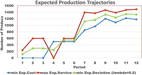
Figure 5. Boundary and viable RMI of part types for $\lambda =0.5$.

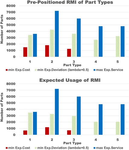
Figure 6. Boundary and viable reserve capacity for $\lambda =0.5$.

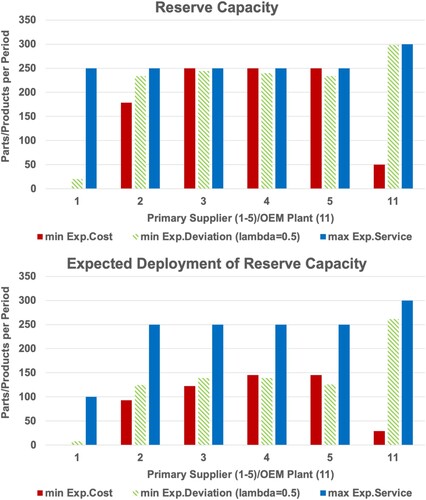
Figure 7. Boundary trajectories and viable expected production schedules for $\lambda =0,0.25,0.75,1$.

Figure 8. Expected shortage of products for viable solutions of Viabil_WD, for $\lambda =0,0.5,1$.

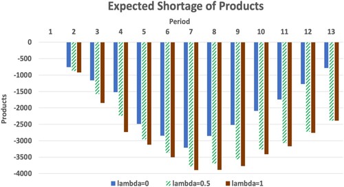
Finally, Figure 8 shows the expected inventory/shortage of products, $\sum _{s\in S}{P}_s{w}_t^s,t\in T^{\ast }$ (see the inventory constraints (22(22) $\begin{array}{rl}& w_{t+1}^s=w_t^s+x_{mt}^s-d_t^s;t\in T,s\in S\end{array}$(22) )–(23(23) $\begin{array}{rl}& w_1^s=0;s\in S\end{array}$(23) )), for viable solutions of Viabil_WD, for $\lambda =0,0.5,1$. The least expected shortage is obtained for $\lambda =0$, for which production coincides with the boundary production for the service-optimal solution. The expected shortage for $\lambda =0.5$ is much greater and closer to solution associated with the cost-optimal boundary production for $\lambda =1$. Note that for the example problems, the greatest expected shortage of products occurs in the middle of the planning horizon, when the supply chain performance is mostly affected by the propagated disruptions. However, in the proposed formulation the manufacturer is charged with penalty cost only for the shortage of products at the end of the planning horizon, i.e. the unfulfilled demand in a dummy period, h + 1 = 13.

For the example problem, the minimum distance (35(35) $\underset{t\in T}{min}\sum _{s\in S}{P}_s|X_t^s-Y_t^s|.$(35) ) between the boundary trajectories, applied to evaluate the supply chain resilience to the ripple effect, is obtained for periods t = 5, 6, when the boundaries are very close to each other: $\sum _{s\in S}{P}_s{X}_t^s=576$ products and $\sum _{s\in S}{P}_s{Y}_t^s=600$ products. Nevertheless, for all weight factors λ, model Viabil_WD generates viable production levels in-between those boundary values (see Table 5).

Table 6 and Figures 9 and 10 illustrate resilient solutions obtained for model Resil_WS. In general, the resilient solutions are similar to the viable solutions presented in Table 5. The resilient and viable expected primary and recovery supply portfolios are identical. However, since the weighted sum objective (36(36) $\lambda \frac{E^c-{\underset{\_}{E}}^c}{{\overline{E}}^c-{\underset{\_}{E}}^c}+(1-\lambda )\frac{{\overline{E}}^{sl}-E^{sl}}{{\overline{E}}^{sl}-{\underset{\_}{E}}^{sl}}$(36) ) of Resil_WS directly optimises expected cost and service, the obtained solution values presented in Table 6 outperform the corresponding values for model Viabil_WD, for most values of λ (see, Table 5). Moreover, the resilient expected production trajectories are different from the corresponding viable trajectories and are very close to each other (cf. Figure 4 vs Figure 10). In addition, Figure 10 indicates that the cost-optimal and the service-optimal resilient trajectories are no longer boundary trajectories. For example, in the first two periods, t = 1, 2, when the smallest distance between the two trajectories (respectively 0, 240–209 = 31 products) occurs, the optimal resilient trajectory for equally important cost and service (for $\lambda =0.5$) lies above the two trajectories. The other differences are observed between the resilient and viable pre-positioning of RMI of parts and the reserve capacities. The resilient solutions lead to a better balanced pre-positioning of RMI for different part types, (cf. Figure 5 vs Figure 9) and a better balanced reserve capacities (cf. Figures 6 vs Figure 9). Overall, the above differences between the viable and resilient solutions are not significant and rather emphasise that supply chain resilience and viability are closely related.

Figure 9. Pre-positioned RMI and reserve capacity for resilient solutions of Resil_WS, for $\lambda =0,0.5,1$.

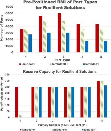
Figure 10. Expected production and shortage for resilient solutions of Resil_WS, for $\lambda =0,0.5,1$.

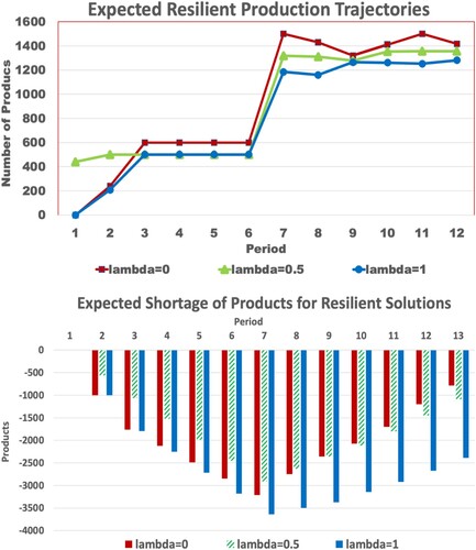
Table 6. Solution results for supply chain resilience model Resil_WS

Weight factor, λ	0	0.25	0.50	0.75	1
Expected Cost ($E^c$)	80.33	79.23	77.50	75.74	75.04
Expected Service Level ($E^{sl}$)	93.47%	93.47%	90.93%	85.79%	80.09%
Expected Primary Supply Portfolio (% of total demand for part type, i) ${}^{\left(\mathrm{b}\right)}$
1(70%), 2(90%), 3(90%), 4(90%), 5(90%)
Expected Recovery Supply Portfolio (% of total demand for part type, i−5) ${}^{\left(\mathrm{c}\right)}$
6(30%), 7(10%), 8(10%), 9(10%), 10(10%)
Expected Resilient Production Trajectory ${}^{\left(\mathrm{d}\right)}$
Period	Production	Production	Production	Production	Production
t = 1	0	520	440	0	0
t = 2	240	520	500	500	209
t = 3	600	520	500	500	500
t = 4	600	520	500	500	500
t = 5	600	520	500	500	500
t = 6	600	520	500	500	500
t = 7	1500	1349	1319	1291	1185
t = 8	1430	1331	1310	1261	1159
t = 9	1320	1302	1278	1262	1265
t = 10	1410	1371	1354	1325	1261
t = 11	1500	1377	1356	1328	1252
t = 12	1417	1377	1356	1328	1281

${}^{\left(\mathrm{a}\right)}$ Var.=6722, Bin.=69, Cons.=8306.

${}^{\left(\mathrm{b}\right)}$ $\sum _{s\in S}{P}_s{g}_i^s;i\le M$.

${}^{\left(\mathrm{c}\right)}$ $\sum _{s\in S}{P}_s{v}_{M+i}^s;i\le M$.

${}^{\left(\mathrm{d}\right)}$ $\sum _{s\in S}{P}_s{x}_{mt}^s;t\in T$.

The computational experiments were performed using the AMPL programming language and the Gurobi 9.5.1 solver on a MacBookPro laptop with Intel Core i7 processor running at 2.8 GHz and with 16 GB RAM. CPU time required for a proven optimal solution was equal to fraction of a second, which is in part due to a very strong LP relaxation of the proposed stochastic MIP model.

6. Concluding remarks

In this paper, a novel quantitative approach was developed for the problem of supply chain viability under the ripple effect propagated from a single disruption source region. The approach exploits the fact that the two main performance measures of supply chain operations, cost and service, are in conflict. As a result, the associated cost-optimal and service-optimal production trajectories can be considered boundaries on all acceptable production trajectories under the ripple effect. Thus instead of viability kernel commonly used in the viability theory, this paper establishes the boundaries on acceptable supply chain states in which the supply chain can continue to exist under the ripple effect and avoid severe losses. For a given implementable portfolio of controls (reservation capacity at primary suppliers and OEM assembly plant, recovery backup supplies of parts to OEM plant and RMI of parts pre-positioned at OEM plant), the boundaries on acceptable production trajectories associated with the two conflicting objectives, cost and customer service level, are determined. In addition, the novel quantitative approach and the developed stochastic quadratic MIP model with a very strong LP relaxation prove very high computational efficiency. The decision maker obtains proven optimal solution (the optimal portfolio of implementable controls) in a very short CPU time, in fraction of a second for the example problems. The basic managerial implication of the proposed approach are listed below,

Managerial implications

• The boundary production trajectories associated with the two conflicting objective functions, cost and service, make the decision maker aware of the extreme policies available to mitigate the impact of the ripple effect.

• The greater the distance between the boundary trajectories, the more viable and resilient the supply chain under the ripple effect.

• The relative importance of the two conflicting objective functions, cost and service, is modelled by the decision maker's weight factor. The resulting production schedule is inclined toward the corresponding boundary trajectory, if one of the objectives is preferable or remains in-between the two boundaries, when both objectives are equally important.

• While keeping a supply chain production trajectory in-between the two boundaries makes the supply chain more resilient to the ripple effect, the supply chain resilience may diminish as the production trajectory approaches a boundary trajectory. Then, a more severe disruption may push the production outside the viability region and cause greater losses.

• A single objective optimisation of supply chain operations, e.g. with respect to the expected cost or to the expected service level only, which pushes production to the boundaries of the viability region cannot be recommended under severe disruption risks.

• The supply chain resilience can be improved by relaxing bounds on available controls, e.g. by allowing for greater reservation capacities, higher levels of RMI or by selecting more efficient and reliable primary and backup suppliers.

The main weakness of the proposed stochastic optimisation approach can be lack of accurate probability estimates for the high-impact, low-probability disruption risks as well as lack of accurate estimates of the various scenario-dependent parameters. In the future research, some of the simplified assumptions described in Section 2 can be relaxed. For example, direct propagation of the ripple effect from a single disruption source region can be relaxed and indirect propagation between adjacent regions allowed. The model for ‘all-or-nothing’ disruptions can be enhanced for the multi-level disruptions and the binomial probability distribution replaced by a multinomial one, e.g. Sawik (2019). In this study only the most important tier-one suppliers and tier-zero assembly plants are considered, which is sufficient for supply chain analysis in the smartphone manufacturing industry, see Kim and Chung (2022). Nevertheless, in the future research the model can be easily extended to account for the higher-tier suppliers (e.g. Sawik 2021), which can be equally important, for example in the automotive industry. The proposed mathematical models can also be applied for both forward and reverse logistics in the supply chain to consider recycling of products used by consumers, which is a common practice, for example in the smartphone industry, e.g. Kim and Chung (2022).

Acknowledgments

The author acknowledges the helpful comments and clarification requests by four anonymous reviewers.

Disclosure statement

No potential conflict of interest was reported by the author(s).

Data availability statement

The data that support the findings of this study are available from the corresponding author, upon reasonable request.

Additional information

Notes on contributors

Tadeusz Sawik

Tadeusz Sawik is a professor of Industrial Engineering and Operations Research in the Department of Engineering, Reykjavik University in Reykjavik, Iceland and at AGH University of Science and Technology in Kraków, Poland. He received the MS degree in Automation Engineering, the PhD degree in Operations Engineering and the Habilitation degree in Operations Research, all from AGH University. He has been a visiting professor in France, Germany, Greece, Japan, Portugal, Spain, Sweden and Switzerland and has served as a research advisor of Motorola for several years. He is a sole author of numerous books, including Analysis and Synthesis of Multivariable Control Systems, AGH University Press 1984, Discrete Optimisation in Flexible Manufacturing Systems, WNT Publishers 1992, Operations Research for Industrial Engineers, AGH University Press 1998, Production Planning and Scheduling in Flexible Assembly Systems, Springer 1998, Scheduling in Supply Chains Using Mixed Integer Programming, Wiley 2011 and Supply Chain Disruption Management Using Stochastic Mixed Integer Programming, Springer 1st edition 2018, 2nd edition 2020, and more than 150 individual articles in many prestigious journals. He has been a recipient of various individual awards for research achievements, including five times of Scientific Excellence Award from the Minister of Science and Higher Education and over 25 times of Scientific Award from the Rector of AGH. In the World's Top 2% Scientists list recently released by Stanford University and published in PLoS Biology, ranked #144 in Operations Research until the end of 2021, and #71 during the single calendar year 2021. His current research interests include logistics and supply chain management, supply chain risk management, cyber and homeland security, planning and scheduling, mixed integer programming, stochastic and combinatorial optimisation.

References

- Aubin, J. P. 1991. Viability Theory. Boston: Birkhäuser.
- Aubin, J. P. 1997. Dynamic Economic Theory: A Viability Approach. Berlin: Springer Verlag.
- Aubin, J. P., A. M. Bayen, and P. Saint- Pierre. 2011. Viability Theory: New Directions. 2nd ed. Berlin: Springer.
- Chowdhury, P., S. K. Paul, S. Kaisar, and M. A. Moktadir. 2021. “COVID-19 Pandemic Related Supply Chain Studies: A Systematic Review.” Transportation Research Part E 148: 102271. doi:10.1016/j.tre.2021.102271.
- Dolgui, A., and J. M. Proth. 2010. Supply Chain Engineering: Useful Methods and Techniques. London: Springer.
- Hosseini, S., and D. Ivanov. 2020. “Bayesian Networks for Supply Chain Risk, Resilience and Ripple Effect Analysis: A Literature Review.” Expert Systems with Applications 161: 113649. doi:10.1016/j.eswa.2020.113649.
- Hosseini, S., D. Ivanov, and A. Dolgui. 2019. “Review of Quantitative Methods for Supply Chain Resilience Analysis.” Transportation Research Part E 125: 285–307. doi:10.1016/j.tre.2019.03.001.
- Ivanov, D. 2021. “Supply Chain Viability and the COVID-19 Pandemic: A Conceptual and Formal Generalisation of Four Major Adaptation Strategies.” International Journal of Production Research 59 (12): 3535–3552. doi:10.1080/00207543.2021.1890852.
- Ivanov, D. 2022a. “The Industry 5.0 Framework: Viability-based Integration of the Resilience, Sustainability, and Human-centricity Perspectives.” International Journal of Production Research. doi:10.1080/00207543.2022.2118892
- Ivanov, D. 2022b. “Viable Supply Chain Model: Integrating Agility, Resilience and Sustainability Perspectives–Lessons from and Thinking Beyond the COVID-19 Pandemic.” Annals of Operations Research 319: 1411–1431. doi:10.1007/s10479-020-03640-6.
- Ivanov, D., and A. Dolgui. 2020. “Viability of Intertwined Supply Networks: Extending the Supply Chain Resilience Angles Towards Survivability. A Position Paper Motivated by COVID-19 Outbreak.” International Journal of Production Research 58 (10): 2904–2915. doi:10.1080/00207543.2020.1750727.
- Ivanov, D., A. Dolgui, and B. Sokolov, eds. 2019. Handbook of Ripple Effects in the Supply Chain. New York: Springer.
- Ivanov, D., and B. B. Keskin. 2022. “Post-pandemic Adaptation and Development of Supply Chain Viability Theory (editorial to Special Issue on Supply Chain Viability).” Omega 116: 102806. doi:10.1016/j.omega.2022.102806.
- Karacaoglu, G., and J. B. Krawczyk. 2021. “Public Policy, Systemic Resilience and Viability Theory.” Metroeconomica 72 (4): 826–848. doi:10.1111/meca.12349.
- Kim, Y. G., and B. D. Chung. 2022. “Closed-loop Supply Chain Network Design Considering Reshoring Drivers.” Omega 109: 102610. doi:10.1016/j.omega.2022.102610.
- Kim, K., and J. B. Krawczyk. 2017. “Sustainable Emission Control Policies: Viability Theory Approach.” Seoul Journal of Economics 30: 291–317.
- Krawczyk, J. B., and K. Kim. 2009. “Satisficing Solutions to a Monetary Policy Problem: A Viability Theory Approach.” Macroeconomic Dynamics 13: 46–80. doi:10.1017/S1365100508070466.
- Krawczyk, J. B., and V. P. Petkov. 2022. “A Qualitative Game of Interest Rate Adjustments with a Nuisance Agent.” Games 13: 58. doi:10.3390/g13050058
- Krawczyk, J. B., A. Pharo, O. S. Serea, and S. Sinclair. 2013. “Computation of Viability Kernels: A Case Study of By-catch Fisheries.” Computational Management Science 10: 365–396. doi:10.1007/s10287-013-0189-z.
- Lücker, F., R. W. Seifert, and I. Bicer. 2019. “Roles of Inventory and Reserve Capacity in Mitigating Supply Chain Disruption Risk.” International Journal of Production Research 57 (4): 1238–1249. doi:10.1080/00207543.2018.1504173.
- Özçelik, G., O. F. Yılmaz, and F. B. Yeni. 2021. “Robust Optimisation for Ripple Effect on Reverse Supply Chain: An Industrial Case Study.” International Journal of Production Research 59 (1): 245–264. doi:10.1080/00207543.2020.1740348.
- Paul, S. K., M. A. Moktadir, K. Sallam, T.-S. Choi, and R. K. Chakrabortty. 2021. “A Recovery Planning Model for Online Business Operations Under the COVID-19 Outbreak.” International Journal of Production Research. doi:10.1080/00207543.2021.1976431.
- Ruel, S., J. El Baz, D. Ivanov, and A. Das. 2021. “Supply Chain Viability: Conceptualization, Measurement, and Nomological Validation.” Annals of Operations Research. doi:10.1007/s10479-021-03974-9
- Sardesai, S., and K. Klingebiel. 2023. “Maintaining Viability by Rapid Supply Chain Adaptation Using a Process Capability Index.” Omega 115: 102778. doi:10.1016/j.omega.2022.102778.
- Sawik, T. 2011. “Selection of Supply Portfolio Under Disruption Risks.” Omega 39: 194–208. doi:10.1016/j.omega.2010.06.007.
- Sawik, T. 2013. “Selection of Resilient Supply Portfolio Under Disruption Risks.” Omega 41 (2): 259–269. doi:10.1016/j.omega.2012.05.003.
- Sawik, T. 2015. “On the Fair Optimization of Cost and Customer Service Level in a Supply Chain Under Disruption Risks.” Omega 53: 58–66. doi:10.1016/j.omega.2014.12.004.
- Sawik, T. 2017. “A Portfolio Approach to Supply Chain Disruption Management.” International Journal of Production Research 55 (7): 1970–1991. doi:10.1080/00207543.2016.1249432.
- Sawik, T. 2019. “Disruption Mitigation and Recovery in Supply Chains Using Portfolio Approach.” Omega 84 (4): 232–248. doi:10.1016/j.omega.2018.05.006.
- Sawik, T. 2020. Supply Chain Disruption Management: Using Stochastic Mixed Integer Programming. New York: Springer.
- Sawik, T. 2021. “On the Risk-averse Selection of Resilient Multi-tier Supply Portfolio.” Omega 101: 102267. doi:10.1016/j.omega.2020.102267.
- Sawik, T. 2022. “Stochastic Optimization of Supply Chain Resilience Under Ripple Effect: A COVID-19 Pandemic Related Study.” Omega 109: 102596. doi:10.1016/j.omega.2022.102596.
- Yılmaz, O. F., G. Özçelik, and F. B. Yeni. 2021. “Ensuring Sustainability in the Reverse Supply Chain in Case of the Ripple Effect: A Two-stage Stochastic Optimization Model.” Journal of Cleaner Production 282: 124548. doi:10.1016/j.jclepro.2020.124548.