On the multi-period combined maintenance and routing optimisation problem

Abstract

This paper focuses on the combined maintenance and routing optimisation problem in a multi-period environment that consists of scheduling maintenance operations for a set of geographically distributed machines, subject to non-deterministic failures with a set of technicians that perform preventive maintenance and corrective operations. This study uses a two-step approach based on column generation. The first step consists of a maintenance model that determines the optimal time until the next preventive maintenance operation, and each machine’s maintenance frequency while minimising the total expected maintenance costs. The second step involves a routing model that assigns and schedules maintenance operations for each technician over the planning horizon while minimising the routing and maintenance costs. We formulate the second step problem as a periodic vehicle routing problem and to solve it, we propose a column generation approach. The master problem is a set partitioning formulation that indicates which machines must be visited in the planning horizon. This decomposition has two auxiliary problems: the first one is an elementary shortest-path problem to find a feasible path for each period and the second one finds a set of visiting periods for each machine. Our approach balances the maintenance cost, routing cost, and failure probabilities.

KEYWORDS:

• Combined maintenance and routing
• column generation
• maintenance planning
• vehicle routing
• waiting time

1. Introduction

Thoughtful planning and scheduling of maintenance operations lead to significant improvements in the reliability of an industrial installation or a distribution network (Remy et al. 2013). Therefore, optimising maintenance planning plays a crucial role in the strategic continuity of operations, several decisions can be optimised such as the frequency of the maintenance actions or the dates when maintenance is scheduled.

Today’s business dynamics demand a high level of operational efficiency and effectiveness where continuity becomes a crucial factor in the business economy. Therefore, maintenance in any productive system ceases to be considered a cost generator that has a negative effect on productivity. It becomes an important factor that can generate value for different operations. Maintenance decisions can be influenced by different factors (Van Horenbeek, Pintelon, and Muchiri 2010) such as policies – (failure-based, time use, condition-based), events (failures, time limits, conditions), actions (corrective, replacement, preventive, preventive replacement), criteria (costs, availability, reliability), effectiveness (perfect repair, minimal repair, imperfect repair, worse repair, worst repair), deterioration (failure distribution, ageing models, condition-based), and system information (complete, incomplete, data sources).

Given these maintenance concepts, the optimisation models become important tools that support decision-making in strategy development that achieves the continuous operation of any production system. By identifying effective policies and special factors, it can be used to optimise the policies of maintenance while satisfying different goals such as cost or reliability. Nevertheless, to guarantee the correct maintenance of any system it is necessary to consider the constraints of this process, which is the personnel or machinery involved in the maintenance process to guarantee the correct maintenance of any system. Therefore, it is important to consider the interrelated problems of maintenance and routing personnel or machines that perform this maintenance.

In many industrial fields the continuity of the production or operational system depends on the multicomponent system and its functionality and the reliability of the overall system can be affected over time if one or more components are not working appropriately (Zhang et al. 2022) (Elsido, Martelli, and Grossmann 2021). In this sense, enterprises are also restricted by costs mainly because the crew that performs this type of work increases the overall costs (Han, Zhen, and Huang 2022) due to the time required to perform the operations (travel and repair times). For example, in systems such as multipurpose process plants, the time period of the maintenance planning is crucial for the operation given that the production plan and the flexibility of the system can be affected (Vassiliadis et al. 2000), other industrial example is related to the maintenance planning of public buildings including risk criteria, (Ruparathna, Hewage, and Sadiq 2018).

López-Santana et al. (2016) proposed the combined maintenance and routing optimisation problem. The authors consider a system with a set of machines that are geographically distributed over a region. These machines are subject to unforeseen failures that result in downtime and hence loss of productivity. To reduce the unforeseen downtimes, a maintenance operation is scheduled with a certain frequency. A set of technicians who are missioned to visit these machines to perform maintenance operations are also considered. When a machine fails suddenly, the maintenance crew must perform Corrective Maintenance (CM) operations.

The applicability of our proposed approach in an industrial context lies in complex systems in which the continuity of the operation is critical for business and performance indicators such as production systems, oil and gas processes, airline industries, and wind power generation systems among others, in fact, some commercial solutions try to solve this type of problems, for instance (IBM 2022).

The remainder of this paper is organised as follows. Section 2 reviews the literature related to combined maintenance and routing problems. In Section 3 the problem statement is presented followed by the mathematical models, Section 4 with the maintenance model, Section 5 with the routing model, and the decomposition approach. Section 6 introduces the benchmark procedure, which consists of a simple method to generate the visit pattern set and it is used to test the relevance of integrating the routing model within the maintenance policies over several periods. The experimentation and analysis are shown in Section 7 and finally, conclusions are developed in Section 8.

2. Literature review

A maintenance policy is the combination of inspections (for monitoring purposes) and preventive and corrective operations intended to restore a machine to a state in which it can perform its required functions Lugtigheid, Banjevic, and Jardine (2004). In this way, this review aims to find the main mathematical models and related factors considered in the planning of maintenance operations. For deeper studies of maintenance optimisation models see (A Review on Maintenance Optimisation 2019).

Several authors have developed applications depending on the type of maintenance and additional characteristics considered. For example, in (Martinod et al. 2018), the authors have developed an optimisation approach for generating maintenance policies in a multiple-product environment. The authors propose an optimisation technique in which the maintenance policy used is defined as an imperfect maintenance action, where actions are divided into corrective and preventive. The main objective is to minimise the preventive and corrective maintenance costs. For the preventive actions, two different policies are evaluated: (i) periodic block-type where maintenance is performed periodically over a planning horizon, and (ii) aged-based policy that uses a reliability function for each component that defines a threshold value for performing the maintenance. The proposed model and policies are tested in a real-life application of passenger-aerial-cable cars.

Another application of maintenance strategies is proposed by (Faddoul, Raphael, and Chateauneuf 2018). The authors consider the interdependencies between multiple components in their application. Over a planning horizon of one year, the deterioration of the components is modelled using Markov decision processes and is solved using a combined stochastic dynamic programming and Lagrangian relaxation. Numerical tests are performed over a pipeline with five serial sections where the deterioration of each component is modelled using several factors. The considered maintenance policies are: (i) do nothing, (ii) preventive, (iii) corrective, and (iv) replacement.

The application of routing personnel and optimisation of the maintenance of airplanes is presented in (Eltoukhy et al. 2018). The authors discerned that aircraft maintenance and maintenance staffing problems are interrelated and interdependent; therefore, they develop a joint mathematical model to solve both problems. By identifying the objectives of both problems as a multi-objective model, the authors have developed a bi-level optimisation programming model embedded with an ant colony optimisation metaheuristic to solve the first stage of the problem. The problem is modelled using a scenario-based approach for the stochastic version, and a strategy of the leader-follower Stackelberg game is used to connect the problems. The model is tested over a real instance of a middle-size airline company to obtain improved cost. Another application of the maintenance of airplanes is presented in (Eltoukhy et al. 2019) where a study of the interdependence of aircraft routing and maintenance staffing is developed. The study uses the concept of Nash equilibrium with Ant Colony Optimisation and data analytics to optimise the selection of maintenance providers to decide the size of the crew and the places where the maintenance is to be performed to minimise the overall cost.

In any system, different limitations are involved when making decisions. Maintenance decisions are affected by these limitations. In (Khatab et al. 2018), the authors proposed an application where a selective maintenance problem is developed by introducing a nonlinear programming model that selects the components to be maintained, the maintenance levels, and the assignments to repair persons or channels. Several samples were tested to prove the benefits of the model’s application.

An application for joint maintenance and production control is presented by (Wakiru et al. 2021). In this paper, the authors integrated opportunistic maintenance by considering several factors that affected the operation and proposing an approach that used discrete event simulation modelling. The study evaluated the stochasticity of different elements of the operation embedded with a semi-Markov decision process and the opportunistic maintenance generating rules for performing the maintenance operations. This proposal also uses degradation rates to evaluate product quality and its relationship with maintenance operations. Similarly (Gopalakrishnan, Subramaniyan, and Skoogh 2020) proposed a data-driven approach to analysing the maintenance operations and increased productivity. Their proposal is based on a framework for evaluating machine criticality where four different cases were evaluated concluding increments in productivity when the proposal is used.

When a system of study includes multiple interrelated components, an application of power systems can be found (Briš et al. 2017). In this paper, the authors distinguished between four types of components: non-repairable, repairable with CM, repairable with latent failures, and reparable with preventive policies. The authors used a discrete maintenance optimisation method with a reliability constraint where the stochastic factor was the life cycle. This proposed method was validated through the use of a real case in a power system network, a similar problem was also analysed in (Foong et al. 2008). Also, a multi-station system was studied in (Zhou & Shi, 2019). The authors modelled the problem by using a capacity function rate to describe the impacts of the failures in the system’s capacity. Based on this function, a rule-based opportunistic maintenance policy was proposed.

Samal and Pratihar (2015) developed a joint optimisation model for the maintenance and spare parts inventory problems. For modelling the life cycle of machines, the authors have used the probability of a failure as a function of time and consider that the time spent repairing a machine is depreciable. Once maintenance is performed, the assumption is that the machine is restored as good as new. The spare kits are required for performing the maintenance and their orders generate costs associated with inventory, holding, and backorders. To solve this combined problem, a genetic algorithm and particle swarm optimisation are used and tested with instances from real cases in the industry generating cost savings.

In the same way (Nguyen et al. 2019), by including routing in the maintenance process, to develop an optimisation model for the maintenance of a production system using the grouping and routing of a crew. The maintenance is divided into two different parts: corrective, using the policy as bad as old, and preventive using the policy as good as new. Grouping and planning maintenance crew routes are solved by a combination of local search and genetic algorithms. Also, the life cycle of each interrelated critical component of the production system is modelled with a Weibull distribution. Several experiments were performed with generated instances, also a sensitivity analysis was performed.

Another application of combined routing and maintenance is presented by (Ade et al. 2017). The authors develop an application for routing and scheduling planning for the maintenance of offshore wind farms. The authors do not consider the life cycle of the wind farms as a stochastic process. However, over a planning horizon, they decide the period to make the maintenance which can be of different types. Routing and scheduling are solved using a MILP and Dantzig-Wolfe decomposition which is solved for each turbine generating feasible paths for each period. Another MILP is proposed for finding the optimal configuration that minimises the total costs.

Hajej, Rezg, and Gharbi (2020) presented a combination of maintenance and production operations in the case of remanufactured products. The authors developed a two-stage mathematical optimisation problem that included the average number of failures in a production cycle as the estimation of the stochastic values. To solve the problem, the use of an evolutionary algorithm was proposed. Similarly (Hajej, Rezg, and Gharbi 2018) proposed a combination of a production system that is subject to failures that can affect the quality of the product. The proposed model determines a joint control policy based on a stochastic production and maintenance planning problem. This work was extended by (Hajej and Rezg 2020) who added a multi-machine environment intended to minimise the overall total costs composed of the production, maintenance, and energy consumption elements.

Similarly (Koochaki et al. 2012) proposed the use of the condition-based rule to perform preventive maintenance operations by a group of maintenance operators. Nevertheless, these operators are considered under different scenarios: (1) an unlimited number of operators, (2) a limited number of operators, and (3) external operators with service times. The performance indicators are related to maintenance costs and how smoothly the maintenance plans are executed.

Jbili et al. (2018) proposed a very interesting problem that performs the maintenance of the vehicles in the routing process. The article’s main idea concerns guaranteeing the distribution process in intercontinental transportation, where critical components of vehicles are subject to failure and the reparation time is unknown. Replacement of failed components is the maintenance policy under consideration, and a mathematical model is proposed to solve small instances while a genetic algorithm is also proposed for bigger instances. A similar problem for the railway corridors was analysed by (Ome et al. 2018) but without considering the crew as a maintenance factor.

A mathematical optimisation model and algorithmic approach for the combined design and maintenance of large-scale multicomponent industrial systems was developed in (Adjoul et al. 2021). The authors have proposed a two-phase algorithm wherein the first part – a Non-Sorting-Genetic Algorithm II (NSGA-II) – is used to identify the best combinations of design solutions and is used as an input for the second phase, which searches a dynamic maintenance planning using a genetic algorithm. The proposed approach was tested over different instances taken from the literature, costs were reduced, and the robustness of the system was improved.

Also in (Ahmed, Zeghal Mansour, and Haouari 2018), a combined problem involving aircraft, maintenance, and crew pairing was developed. The main idea was to find an aircraft route maintenance policy and a crew pairing to support the maintenance. Because these two decisions are interrelated, the authors proposed to find robust solutions that can respond to unpredictable disruptions such as weather and breakdowns. The authors used information from well-known companies to test their approach and have generated a set of circumstances that showed good quality, cost-effective solutions.

Table 1 presents a classification of the main characteristics of the articles analysed above given two major elements: (i) maintenance and (ii) technicians which has its own main characteristics.

Table 1. Summary and classification of the literature review.

	Maintenance characteristics							Technician characteristics
Article	Multi-period Planning	Multi-machines	CM	PM	Random time to failure	Machines geographically distributed	Without Degradation	Scheduling (visits patterns)	Routing	Travel Times	Time Windows	Workload	Combined Maintenance and Technicians
Martinod et al. 2018	X	x	x	x	X		x
Faddoul, Raphael, and Chateauneuf 2018	X	x	x	x
Eltoukhy et al. 2018		x		x			x	x				x	x
Eltoukhy et al. 2019	X	x		x			x					x
Khatab et al. 2018		x	x	x
Wakiru et al. 2021		x	x	x	X
Gopalakrishnan, Subramaniyan, and Skoogh 2020		x	x	x		x	x
Briš et al. 2017		x	x	x	x
Foong et al. 2008	X	x	x
Zhou & Shi 2019		x		x	x
Samal and Pratihar 2015		x			x		x
Nguyen et al. 2019	X	x	x	x	x	x	x	x	x	x			x
Irawan et al. 2017	X	x	x	x				x	x	x			x
Hajej, Rezg, and Gharbi 2020	X	x	x	x
Hajej, Rezg, and Gharbi 2018				x	x		x
Hajej and Rezg 2020		x		x	x		x
Koochaki et al. 2012	X			x	x					x			x
Jbili et al. 2018	X	x	x	x	x
Ome et al. 2018	x	x	x	x	x
Adjoul et al. 2021		x	x
Ahmed, Zeghal Mansour, and Haouari 2018	x	x	x	x				x	x	x			x
Our approach	x	x	x	x	x	x	x	x	x	x	x	x	x

Based on the articles analysed in Table 1, the main contribution of our work can be summarised as follows: from the managerial perspective, the optimisation models become an important tool that supports decision-making in the strategic development that achieves the continuous operation of any production system. Therefore, we have included in our analysis four main elements that affect the maintenance planning process: multiple time periods, random times of failure, geographically distributed machines, and the condition of the machines after a CM or PM operation. These real elements are in most of the works described in the literature discussed. By identifying the policies and special factors to use, our analysis can become a tool that optimises the maintenance policies while satisfying different criteria such as costs or reliability. Nevertheless, to guarantee the correct maintenance of any system it is necessary to consider a limiting factor for this process, which is the personnel or machinery involved in the maintenance process. Therefore, it is important to consider the interrelated problems of maintenance and routing personnel or machines that perform this maintenance. From this point of view, we have included real aspects of crew scheduling and routing that most of the works described have not included. These factors are related to the scheduling and routing of technicians, the travel times, the time windows, and the workload. Hence, another contribution is the combination of these interrelated decisions that most of the articles treat as separate problems.

From the theoretical perspective, we have extended the work developed by (López-Santana et al. 2016) by increasing the complexity of the model by adding multiple time periods. Also, we have modified the basic model where we have eliminated the connection between the RM and the MM by leaving the expected waiting time which is a stable variant of the maintenance model. In addition, we propose a solution approach based on column generation decomposition approach with two subproblems. The first subproblem generates feasible paths for the technicians to visit the machines, and the second one makes the pattern visit to schedule the maintenance operations in the planning horizon.

3. Problem statement

López-Santana et al. (2016) introduces the CMR optimisation problem. The authors consider a system with a set of customers $V_C=\left\{1,2,\dots ,N\right\}$ geographically distributed over a region, where each customer has one machine subject to unforeseen failures. The machines are mutually independent regarding their failures and hence it is possible to determine an optimal maintenance policy for each machine separately. To reduce the occurrence of these unforeseen failures, maintenance operations are scheduled with a certain frequency for each machine in a planning horizon. We extended the CMR optimisation problem in a planning horizon $\mathcal{T}$ defined by a set of periods $\left\{1,2,\dots ,\mathcal{T}\right\}$, for instance, days in a week. For each period $t\in \mathcal{T}$ we consider a set of identical technicians $K=\left\{1,2,..,m\right\}$, who need to visit the set of machines to perform the scheduled maintenance operations. In addition, the technician performs a CM operation in cases where the machine fails suddenly before the scheduled date of the maintenance operation. A single central depot indexed by $0$ (outside of all customer locations) is considered as the point of departure and the final destination for all technicians. Thus our problem can be defined in a directed complete graph $G=\left(V,A\right)$, $V=V_C\cup \left\{0\right\}$, $A=\left\{\left(i,j\right):i,j\in V,i\ne j\right\}.$ Each arc $\left(i,j\right)$ has an associated non-negative value $d_{ij}$ which represents the travel time from $i$ to $j$. Finally, the multi-period combined maintenance and routing optimisation problem (MP-CMR) consists of determining a joint routing-maintenance policy for all machines such that it minimises the routing cost and the total expected maintenance cost (PM and CM costs including the cost of unavailability due to the delay time before the arrival of the technician in case of failure). The assumptions and conditions of the problem are summarised as follows:

• The machines are mutually independent in terms of failure behaviour.

• The machines start in as good as new condition, and after the PM or CM operation, they are returned to as good as new condition.

• A cycle is the time interval between two renewals of the machine, i.e. a cycle starts after the completion of the PM or CM operation and ends when the next PM or CM operation is performed.

• The mean time required to perform a CM operation is longer than the mean time required to perform a PM operation on each machine.

• The CM cost is higher than the PM cost.

• It is possible to schedule a maximum of one maintenance operation in each period for each customer.

• All technicians are homogeneous in the sense that they can perform any PM or CM operation and the travel times between any given pair of customers are identical (among all technicians).

• For all periods, all technicians start in the depot at the beginning of the planning horizon and must return to the depot by the end of the planning horizon.

• The travel times are deterministic and fulfil the triangle inequality.

• In the case of failure before the beginning of the next maintenance operation, the customer must wait for the technician, i.e. the technician is not rescheduled based on the customer’s new situation.

According to (López-Santana et al. 2016), our approach consists of solving two models:

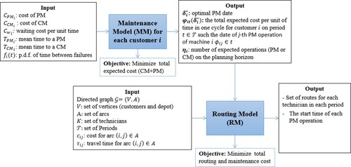
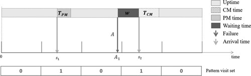
1. Maintenance Model (MM): for each customer, we solve the MM introduced by (López-Santana et al. 2016). The input of this model is the set of parameters shown in Figure 1. The MM allows determining the optimal date of a maintenance operation. This optimal time is calculated by minimising the individual total expected maintenance policy costs per unit of time (CM and PM). Given the planning horizon, the output consists of the number of maintenance operations, the date that each operation should be executed, and the expected maintenance policy cost for each period $t\in \mathcal{T}$.

2. Routing Model (RM): This model takes as input the outputs of the MM, the set of periods $\mathcal{T}$ and the graph $G=\left(V,A\right)$ corresponding to the geographical location of the customers and the depot as an input (see Figure 1). For the RM, we use a column generation approach to find a set of routes (also named paths) such that all maintenance operations are executed, and the route duration does not exceed the available workload of each technician and each period. The output is a set of routes for each technician in each period, with the scheduled maintenance operations.

Figure 1. Proposed Multi-Period Combined Maintenance and Routing (MPCMR) model.

Algorithm description composed by two inputs, two outputs, and their connection between the Maintenance Model (MM) and Routing Model (RM).

The notation used in the maintenance and routing models is as follows:

Sets:

$V_C$:	=	set of customers
$V$:	=	set of vertices (customers and depot)
$A$:	=	set of arcs
$K$:	=	set of technicians
$\mathcal{T}$:	=	set of periods
$R:$	=	set of visit patterns
$v_i$:	=	set of PM operations of customer i, ${\nu }_i=\left\{o_i^1,o_i^2,..,o_i^{{\eta }_i}\right\}$

Parameters:

$\mathcal{T}{}^{\mathrm{\prime }}$:	=	planning horizon
$N$:	=	number of customers
$m$:	=	number of technicians
$T_i:$	=	random variable of the time to failure of machine $i$
$f_i\left(T_i\right):$	=	probability density function (p.d.f.) of $T_i$
$F_i\left(T_i\right)$:	=	cumulative distribution function of $T_i$
${\delta }_i$:	=	maintenance operation period of machine $i$
$w_i\left({\delta }_{\text{i}}\right):$	=	expected waiting time in function of maintenance operation period ${\delta }_i$ of machine $i$
$r_{ik}^t:$	=	the renewal time before the maintenance operation $i$ when it is performed by technician $k$ in a period $t$
$s_{jk}^t$:	=	start time of a maintenance operation $j$ when it is performed by technician $k$ in a period $t$
$M_i\left({\delta }_i\right)$:	=	conditional expected time to failure of machine $i$ when the maintenance operation is ${\delta }_i$ knowing that the failure occurs before ${\delta }_i$
${T_{CM}}_i$:	=	mean time required to perform a CM operation of machine $i$
${T_{PM}}_i$:	=	mean time required to perform a PM operation of machine $i$
${C_{PM}}_i$:	=	the total cost of PM for machine $i$ over its operation
${C_{CM}}_i$	=	the total cost of CM operation for machine $i$ over its operation
${C_w}_i$:	=	waiting cost per unit time at machine $i$
${\mathcal{C}}_i\left({\delta }_i\right)$:	=	the total expected cost per unit of time incurred in one cycle for machine $i$ when the maintenance operation period is ${\delta }_i$
${\phi }_t$:	=	expected maintenance cost per unit of time in a period $t$
${\phi }_{it}$:	=	expected maintenance cost per unit of time for machine $i$ in a period $t$
${\phi }_{ir}$:	=	expected maintenance cost per unit of time for machine $i$ in a visit pattern $t$
${\eta }_i$:	=	number of expected operations (PM or CM) on the planning horizon for machine $i$
${\varphi }_{ij}$:	=	date of j-th PM operation of machine $i$ ($j\in {\nu }_i$)
${\varphi }_j$:	=	expected date of j-th PM operation
${\tau }_{ij}$:	=	travel time between customers $i$ and $j$

Our proposed approach (multi-period combined maintenance and routing model, MP-CMR) is an extension of the CMR model proposed by (López-Santana et al. 2016) involving multiple periods for the RM and the routing cost in the objective functions. According to (Fontecha et al. 2020), the connection between the MM and the RM was eliminated by leaving the expected waiting time, i.e, $w_i={\delta }_i-M\left({\delta }_i\right)$, which is a stable variant of the MM.

In sections 4 and 5, the components of the MP-CMR model are presented. First, we presented the MM for a single machine and generalised it in the context of geographically distributed machines. Then we developed the RM to schedule maintenance operations and solved it based on a column generation approach.

4. Maintenance model (MM)

We use the maintenance model for one machine introduced by (López-Santana et al. 2016) and modified by (Fontecha et al. 2020). The notation of the MM for a single machine is summarised as follows:

• ${\mathcal{T}}^{\mathrm{\prime }}$: planning horizon

• $T:$ random variable of the time to failure

• $f\left(T\right)$: probability density function (p.d.f.) of $T$

• $F\left(T\right)$: cumulative distribution function of $T$

• $\delta$: maintenance operation period at the beginning of the cycle

• $w$: expected waiting time before the beginning of the CM operation

• $s:$ start time of a maintenance operation

• $M\left(\delta \right)$: the conditional expected time to failure when the maintenance operation period is $\delta$ knowing that the failure occurs before $\delta$

• $T_{CM}$: mean time required to perform a CM operation

• $T_{PM}$: mean time required to perform a PM operation

• $C_{PM}$: total cost of PM operation over its operation

• $C_{CM}$: total cost of CM operation over its operation

• $C_w$: waiting cost per unit time

• $\mathcal{C}\left(\delta \right)$: total expected cost per unit of time incurred in one cycle when the maintenance operation period is $\delta$

• ${\phi }_t$: expected maintenance cost per unit of time in a period $t$

The operation of the machine follows a replacement model, and we define a cycle as the time interval between two renewals of the machine with two types of cycles, preventive, and corrective. For the preventive cycle type, if the machine does not fail before $\delta$ then a PM operation is performed. For the failure cycle type, if the machine fails before time $\delta$ it must wait to be repaired. In Figure 2, the machine starts at time $0$ in as good as new condition and works until time $\delta$, when it undergoes PM and comes back in as good as new condition at time $\delta +T_{PM}$. Therefore, that the first cycle is a preventive cycle and a cost $C_{PM}$ is incurred.

Figure 2. Sample maintenance cycles with preventive and corrective maintenance operations (E. López-Santana et al. 2016).

Three cumulative functions for three different cases of maintenance.

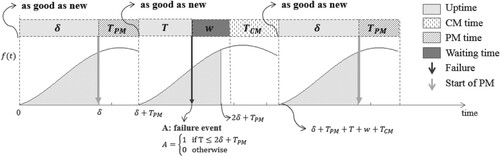
For example, given the machine no fails, then it starts in as good as new condition, then during the second cycle, a failure occurs at time $\delta +T_{PM}+T$, denoted by $A$, then the machine remains unavailable from this date until the next maintenance operation (with the waiting time $w$). After the repair, the machine is assumed to be in as good as new condition again at time $\delta +T_{PM}+T+w+T_{CM}$. In this case, the cycle is a failure cycle and a cost $C_{CM}+w{C}_w$ is incurred, where the first term is the cost of the CM operation, and the second term is the cost of unavailability of the machine because of the waiting time before the CM operation. The third cycle is identical to the first cycle; however, it does not mean that the preventive and corrective maintenance are done continuously one after the other.

The probability of failure in the interval $\left[0,\delta \right]$ is $F\left(\delta \right)$ which is calculated as follows (1) $F\left(\delta \right)=P\left(T\le \delta \right)={\int }_0^{\delta }f\left(t\right)dt.$(1) The probability that a preventive cycle (cycles 1 and 3 in Figure 2) occurs is $1-F\left(\delta \right)$ and the probability that a failure cycle (cycle 2 in Figure 2) occurs is $F\left(\delta \right)$. With the assumption that the machine is in as good as new condition after the PM or CM operation, the cumulative distribution function of failure in any cycle is $F\left(\delta \right)$.

The objective is to determine the optimal maintenance operation period (${\delta }^{\ast }$) that minimises the cost criterion. For this purpose, it is common to use a long-run expected cost per unit time (Jardine and Tsang 2005; López-Santana et al. 2016; Ross 2006). This cost for one machine is given by (2) $\mathcal{C}\left(\delta \right)=\frac{E\left[C\left(\delta \right)\right]}{E\left[T\left(\delta \right)\right]}=\frac{Totalexpectedcostofacycle}{Expectedcyclelength}.$(2) where the total expected cost of a cycle and the expected cycle length is given by equations (3) and (4) according to (López-Santana et al. 2016). (3) $\begin{array}{rl}E\left[C\left(\delta \right)\right]& =C_{PM}\left(1-F\left(\delta \right)\right)+\left(C_{CM}+w{C}_w\right)F\left(\delta \right)\end{array}$(3) (4) $\begin{array}{rl}E\left[T\left(\delta \right)\right]& =\left(\delta +T_{PM}\right)\left(1-F\left(\delta \right)\right)\\ & +\left(M\left(\delta \right)+w+T_{CM}\right)F\left(\delta \right)\end{array}$(4) According to (Fontecha et al. 2020), the expected waiting time $w$ is replaced by $\delta -M\left(\delta \right)$ in equations (3) and (4). In addition, Lopez-Santana et al. (2016) shows as it is computed the mean time to failure $M\left(\delta \right)$ when the maintenance operation is scheduled at time $\delta$ in equation (5). (5) $M\left(\delta \right)={\int }_0^{\delta }\frac{tf\left(t\right)}{F\left(\delta \right)}dt,$(5) Finally, the total expected cost per unit time for a machine is given by: (6) $\mathcal{C}\left(\delta \right)=\frac{C_{PM}\left(1-F\left(\delta \right)\right)+\left(C_{CM}+\left(\delta -M\left(\delta \right)\right)C_w\right)F\left(\delta \right)}{\left(\delta +T_{PM}\right)\left(1-F\left(\delta \right)\right)+\left(\delta +T_{CM}\right)F\left(\delta \right)}.$(6) $\mathcal{C}\left(\delta \right)$ is a continuous convex function for $\delta >0$ given $f\left(t\right)$ and $F\left(t\right)$ are continuous, and $T_{PM}$ and $T_{CM}$ are deterministic and non-negative. According with (Fontecha et al. 2020), the $\underset{\delta \to 0^{+}}{lim}\mathcal{C}\left(\delta \right)=\frac{C_{PM}}{T_{PM}}$ and $\underset{\delta \to \mathrm{\infty }}{lim}\mathcal{C}\left(\delta \right)=C_w$ ensure the feasibility of $\mathcal{C}\left(\delta \right)$. Then, it is possible to determine that this function has a minimum value in some point ${\delta }^{\ast }$. The optimal value of $\delta$ i.e. ${\delta }^{\ast }$ is found from equation (6) using a simple one-dimensional procedure for unconstrained nonlinear optimisation (López-Santana et al. 2016). This procedure uses a straightforward implementation of a golden search method and numerical approximation of the first derivative.

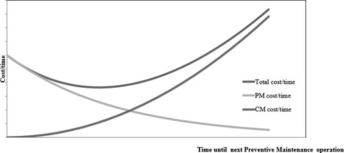
Figure 3 illustrates the curve of cost of the proposed MM. The PM cost decreases as $\delta$ increases since a smaller number of PM operations are required to be performed on the machine over the planning horizon. On the other hand, the CM cost increases when $\delta$ increases since a larger number of CM operations are required at the machine in the planning horizon because the probability of failures increases with $\delta$. The total cost curve is the sum of the PM and CM costs. The date ${\delta }^{\ast }$ (minimum value of $\mathcal{C}\left(\delta \right)$) represents a balance between preventive maintenance and corrective maintenance costs.

Figure 3. Total maintenance policy cost, PM, and CM cost.

Three different graphs of the total costs, preventive maintenance, and corrective maintenance.

If the planning horizon has the length $\mathcal{T}$, then $\eta$ is defined as the frequency of maintenance operations given by: (7) $\eta =\frac{\mathcal{T}}{E\left[T\left({\delta }^{\ast }\right)\right]},$(7) where $\lfloor .\rfloor$ is the floor function and $E\left[T\left({\delta }^{\ast }\right)\right]$ is the expected cycle length at the optimal maintenance time ${\delta }^{\ast }$. For the j-th PM operation over the planning horizon,$j=1,2,\dots ,\eta$, the expected execution date, denoted by ${\varphi }_j$, is calculated as follows: (8) ${\varphi }_j={\delta }^{\ast }+\left(j-1\right)E\left[T\left({\delta }^{\ast }\right)\right]$(8) For the j-th PM operation, we obtain an expected date ${\varphi }_j$ to perform it. We assume that the optimal cost of the maintenance policy remains unchanged when the date of a maintenance operation is shifted from ${\delta }^{\ast }$ to ${\varphi }_j$, thus we set ${\mathcal{C}}_j\left({\varphi }_j\right)=\mathcal{C}\left({\delta }^{\ast }\right)$.

We assume that the planning horizon $\mathcal{T}{}^{\mathrm{\prime }}$ is discretized in a set of periods $\mathcal{T}=\left\{1,2,\dots ,\left|\mathcal{T}\right|\right\}$ and we assume that just one maintenance operation can be scheduled for one period $t$. Then, the length of each period $t$ is $\frac{{\mathcal{T}}^{\mathrm{\prime }}}{\left|\mathcal{T}\right|}$ and the curve of the total expected cost per unit time ${\mathcal{C}}_j\left({\varphi }_j\right)$ is in Figure 4. This situation illustrates the case of 12 periods and 2 PM operations in the planning horizon for one customer.

Figure 4. Approach to the total expected cost per unit time function with |T| = 12 periods and η = 2.

Time horizon composed by 12 time periods with a frequency of two preventive maintenance operations.

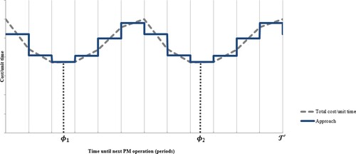
The approximated curve represents the expected maintenance cost per unit time for one customer in a period $t$, denoted by ${\phi }_t$. Given ${\varphi }_{t-1}$ as the lower bound of time and ${\varphi }_t$ as the upper bound of time for a period $t$, the cost ${\phi }_t$ is calculated by (9) ${\phi }_t=\frac{{\mathcal{C}}_i\left({\varphi }_{t-1}\right)+{\mathcal{C}}_i\left({\varphi }_t\right)}{2},t\in \mathcal{T}$(9) The MM presented above is solved for each customer $i\in V_C$, and to generalise this model for $N$ customers an index $i$ is added to all variables. To sum up, for each customer $i$ we obtain the optimum time ${\delta }_i^{\ast }$ until the next maintenance operation, the expected maintenance cost per unit of time ${\phi }_{it}$, and the number of expected operations (PM or CM) on the planning horizon ${\eta }_i$. These are inputs to the RM as described in the next section.

5. Routing model (RM) for PM operations scheduling in a multi-period environment

In this section, we formulate a mixed-integer program to determine the set of routes to be performed by a set of technicians who execute all PM and CM operations over the set of periods of the planning horizon. First, we introduce the mathematical formulation of the routing problem as a multi-period distance-constrained vehicle routing problem and probabilistic constraints. Then, we present a column generation approach to solve the deterministic case.

5.1. The mathematical formulation of the RM

We extended the CMR optimisation problem introduced by (López-Santana et al. 2016) in a multi-period environment defined by a set of periods $\mathcal{T}$. We consider a directed complete graph $G=\left(V,A\right)$, where the vertex set $V=\left\{0,1,2,\dots ,N\right\}$ contains a central depot (vertex $0$), and a subset of customers $V_C=V\mathrm{\setminus }\left\{0\right\}$, as well as the arc set $A=\left\{\left(i,j\right):i,j\in V,i\ne j\right\}$ which represents the links between all pairs of vertices. The technician set is also defined by $K=\left\{1,2,\dots ,m\right\}$. Non-negative weights ${\tau }_{ij}$ are associated with each arc $\left(i,j\right)\in A$; representing the travel time of technicians from customer $i$ to $j$. We assume that these times are given by the shortest-paths and therefore satisfy the triangle inequality. Furthermore, they are assumed to be symmetric ($t_{ij}=t_{ji}\mathrm{\forall }i\ne j$). Each vertex $i\in V_C$ has a duration of the PM operation $T_{PM}$ and the CM operation $T_{CM}$. These features are the same for any period $t$ in the planning horizon.

From the MM, for each customer $i$ we have the number of maintenance operations (${\eta }_i$) over the planning horizon and the expected maintenance cost per unit of time in a period $t$(${\phi }_{it}$). We define a set of visits in a pattern $R_i$ that represents the combinations of visit periods for each customer $i$. For instance, in a set of three periods, the visit pattern $r_1=\left\{1,1,1\right\}$ consists of visiting the customer during all periods and another pattern $r_2=\left\{1,0,1\right\}$ consists of visiting the customer in the periods one and three. Thus, we define ${\text{β}}_{irt}$ as a parameter that is 1 if a period $t$ belongs to visit combination $r\in R_i$ of customer $i$, and 0 otherwise, and ${\phi }_{ir}$ is the expected maintenance cost for a customer $i$ and a visit pattern $r\in R_i$ which is computed by (10) ${\phi }_{ir}=\sum _{t\in \mathcal{T}}{\phi }_{it}{\text{β}}_{irt}.$(10) Moreover, we define an auxiliary set of maintenance operations for customer $i$ as ${\nu }_i=\left\{o_i^1,o_i^2,..,o_i^{{\eta }_i}\right\}$; we further assume $\left|{\nu }_i\right|\ge 1$, which means that at least one PM operation is scheduled over the planning horizon. In addition, we define a set of all maintenance operations $V_M=\sum _{i=1}^N{\nu }_i=\left\{1,2,\dots ,n\right\}$, where $n=\sum _{i=1}^N{\eta }_i$ is the total number of maintenance operations.

Then, the routing problem is defined on the auxiliary directed graph $G^{\mathrm{\prime }}=\left(V^{\mathrm{\prime }},A^{\mathrm{\prime }}\right)$, with $V^{\mathrm{\prime }}=V_C\cup \left\{0,N+1\right\}$ and $A^{\mathrm{\prime }}=\left\{\left(0,i\right):i\in V_C\right\}\cup \left\{\left(i,N+1\right):i\in V_C\right\}\cup \left\{\right(i,j):i,j\in V_C,i\ne j\}$. The nodes 0 and $N+1$ represent the depot. We assume a zero-service time at the depot, that is ${T_{PM}}_0={T_{PM}}_{n+1}=0$ and ${T_{CM}}_0={T_{CM}}_{n+1}=0$. To build the mathematical formulation, two additional sets are defined: ${\mathrm{\Delta }}^{+}\left(i\right)$ called the forward star of vertex $i$, defined as the set of vertices $j$ such that arc $\left(i,j\right)\in A^{\mathrm{\prime }}$, i.e. the vertices that are directly reachable from $i$ (also called successors of $i$). Analogously, ${\mathrm{\Delta }}^{-}\left(i\right)$ denotes the backward star of vertex $i$, defined as the set of vertices $j$ such that arc $\left(j,i\right)\in A^{\mathrm{\prime }}$, i.e. the vertices from which $i$ is directly reachable (predecessors of $i$).

The RM consists of designing a set of routes for each technician such that:

• Each maintenance operation is performed a maximum of one for each period,

• The number of maintenance operations must be greater than or equal to ${\eta }_i$ over the planning horizon

• Every route originates at vertex $0$ and ends at vertex $N+1$ or each period,

We formulate the RM as Multi-period and Distance-Constrained Vehicle Routing Problem (MPDCVRP). We use binary variables $x_{ijk}^t$ that takes the value of 1 only if the technician $k\in K$ on period $t\in \mathcal{T}$ traverses the arc $\left(i,j\right)\in A^{\mathrm{\prime }}$, where $i\ne j$; and take the value of 0, otherwise. Another binary variable is $y_{irk}$ that takes the value of 1 only if customer $i\in V_C$ is visited by technician $k\in K$ on pattern $r\in R_i$; and take the value of 0, otherwise. The variables $s_{ik}^t$ is the start time of maintenance operation on customer $i\in V_C$ when performed by technician $k\in K$ on a period $t\in \mathcal{T}$.

Finally, The RM can then be stated mathematically as follows: (11) $Min\sum _{t\in \mathcal{T}}\sum _{k\in K}\sum _{\left(i,j\right)\in A}{c}_{ij}{x}_{ijk}^t+\sum _{k\in K}\sum _{r\in R_i}\sum _{i\in V_C}{\phi }_{ir}{y}_{irk}$(11) s.t., (12) $\begin{array}{rl}& \sum _{k\in K}\sum _{r\in R_i}{y}_{irk}=1\mathrm{\forall }i\in V_C\end{array}$(12) (13) $\begin{array}{rl}& \sum _{t\in \mathcal{T}}\sum _{k\in K}\sum _{r\in R_i}{\text{β}}_{irt}{y}_{irk}\ge {\eta }_i\mathrm{\forall }i\in V_C\end{array}$(13) (14) $\begin{array}{rl}& \sum _{k\in K}\sum _{j\in {\mathrm{\Delta }}^{+}\left(i\right)}{x}_{ijk}^t=\sum _{k\in K}\sum _{r\in R_i}{\text{β}}_{irt}{y}_{irk}\mathrm{\forall }i\in V_C,t\in \mathcal{T}\end{array}$(14) (15) $\begin{array}{rl}& \sum _{j\in {\mathrm{\Delta }}^{-}\left(i\right)}{x}_{jik}^t-\sum _{j\in {\mathrm{\Delta }}^{+}\left(i\right)}{x}_{ijk}^t=0\mathrm{\forall }i\in V_C,k\in K,t\in \mathcal{T}\end{array}$(15) (16) $\begin{array}{rl}& \sum _{j\in {\mathrm{\Delta }}^{+}\left(0\right)}{x}_{0jk}^t=1\mathrm{\forall }k\in K,t\in \mathcal{T}\end{array}$(16) (17) $\begin{array}{rl}& \sum _{j\in {\mathrm{\Delta }}^{-}\left(n+1\right)}{x}_{j,N+1,k}^t=1\mathrm{\forall }k\in K,t\in \mathcal{T}\end{array}$(17) (18) $\begin{array}{rl}& s_{ik}^t+{T_{PM}}_i\left(1-F_i\left({\delta }_i^{\ast }\right)\right)+{T_{CM}}_i{F}_i\left({\delta }_i^{\ast }\right)+{\tau }_{ij}\\ & -M\left(1-x_{ijk}^t\right)\le s_{jk}^t\mathrm{\forall }\left(i,j\right)\in A,k\in K,t\in \mathcal{T}\end{array}$(18) (19) $\begin{array}{rl}& x_{ijk}^t\in \left\{0,1\right\}\mathrm{\forall }\left(i,j\right)\in A,k\in K,t\in \mathcal{T}\end{array}$(19) (20) $\begin{array}{rl}& y_{irk}\in \left\{0,1\right\}\mathrm{\forall }i\in V_C,r\in R_i,k\in K\end{array}$(20)

The objective function (11) minimises the total routing and maintenance policy cost. The first term in the objective function is the total routing costs that consider the visiting cost of all customers in the paths. The second term consists of the total maintenance policy cost of all PM operations scheduled. Constraints (12) ensure that each customer $i$ is assigned to exactly once visit pattern set over the planning horizon. The visiting pattern set $R_i$ determines in which periods the technician must be to perform a PM or CM operation in the customer $i$. The set of constraints in Equation (13) states that for each customer $i$ that the number of maintenance operation scheduled over the planning horizon is greater than or equal to ${\eta }_i$. The set of constraints (14) links the route variables $x_{ijk}^t$ with the visit pattern $y_{irk}$ to build a feasible route for the technicians over the planning horizon. The set of constraints (15) ensures that after a technician arrives at the vertex $i$ it must leave to another destination. The set of constraints (16) and (17) indicate that each technician must leave the depot (node 0) and must arrive at the depot (node $N+1$) for each period $t$. Note that an unused technician visit is modelled by using the “empty” route $\left(0,N+1\right)$ with ${\tau }_{0,N+1}=0$. The set of constraints (18) establishes the relationship between the technician’s departure time from a customer and its immediate successor where $M$ is a large number. If one route includes visit customer $i$ and $j$, the time include the duration of maintenance operation of customer $i$ plus travel time between customers $i$ and $j$. According with (López-Santana et al. 2016) the duration of a maintenance operation could be a PM or a CM operation, this duration is an expected time dependent on the probability of failure in the last cycle. To approximate this time, we use the probability of a failure in the interval $\left[0,{\delta }_i^{\ast }\right]$ and the expected cycle length as (4). Finally, the set of constraints (19) and (20) impose binary conditions on the flow and visit pattern variables, respectively.

The RM formulation is a deterministic linear combinatorial optimisation problem and it is very hard to solve due to the combination of a DCVRPTW problem which is difficult to solve for larger instances (Kek, Cheu, and Meng 2008; López-Santana et al. 2016), and the set of visit patterns $R_i$ that is too large to consider (Francis, Smilowitz, and Tzur 2008; Rodriguez, Correa, and López-Santana 2015). Thus, we consider a decomposition approach based on a set-covering formulation for the RM and column generation method to find the routes and the visit pattern to scheduling the maintenance operation.

5.2. Decomposition approach to RM

The column generation method is an efficient algorithm for solving larger linear programs (Nemhauser 2012). The main idea of this method consists of exploiting the structure of the problem and only considering a subset of variables (columns) to solve an optimisation problem.

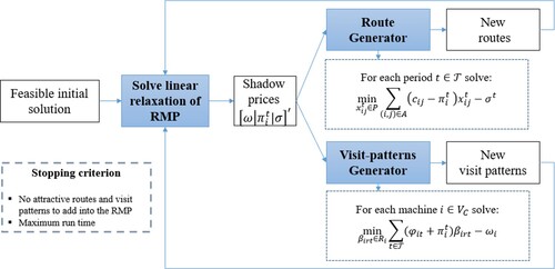
The proposed method solves iteratively two problems: the master problem (MP) and the subproblem (sP). The MP is the original problem with a small subset of variables as the initial solution, it is called the restricted master problem (RMP). With the RMP’s solution and its shadow prices (or dual variables), the sP is created. The sP consists of a new problem created to identify a new attractive variable to add to the RMP. The new variable (column) is added to the RMP if it could improve the RMP’s objective function, i.e. the objective function of the sP is the reduced cost of a new variable concerning the RMP’s shadow prices, and the constraints ensure a feasible solution. Then, the RMP is re-solved again, and the process continues iteratively to the sP returns a solution (column) that does not improve the RMP’s objective function. Hence, it can be concluded that the solution to the MP is optimal. Column generation has also been applied to integer problems. For this, we use the linear relaxation of the restricted master problem (RMP).

The applications in routing problems of the decomposition have successfully been applied in VRPTW and periodic VRP (Choi and Tcha 2007; Grigoriev, Van de Klundert, and Spieksma 2006; López-Santana, Romero Carvajal, and de 2015; Toth and Vigo 2002).

Our approach consists of a Restricted Master Problem (RMP) for the RM formulated as a set-covering problem. We start with a feasible initial solution and solve the linear relaxation of RMP and obtain the shadow prices of each constraint. Then we solve two independent subproblems: a route generator and visit patterns generator. The first subproblem consists of a route generator that is formulated as an Elementary Shortest Path Problem (ESPP) for each period $t\in \mathcal{T}$. The second subproblem is a visit patterns generator for each customer that finds the best allocation of maintenance operations over the planning horizon. The new routes and visit patterns are added into the RMP and re-solved again. This is an iterative process where the stopping criterion can be the lack of improvement in the RMP’s objective function or when the iterative process reaches a maximum allowed run time. Figure 5 illustrates our proposed approach.

Figure 5. Column generation approach to solve the RM.

Squares describing the column generation approach with two subproblems Route generator and Visit-patterns generator and the Master Problem.

5.2.1. The master problem (MP)

P is defined as the set of all feasible routes, where a feasible route starts and ends at the depot (Toth and Vigo 2002). Appendix A describes the way to transform the RM to a set-covering formulation to obtain the master problem.

The resulting model given here is the classical set partitioning formulation: (21) $\begin{array}{r}Min\sum _{t\in \mathcal{T}}\sum _{p\in P}{c}_p^t{z}_p^t+\sum _{r\in R_i}\sum _{i\in V_M}{\phi }_{ir}{y}_{ir}\end{array}$(21) Subject to, (22) $\begin{array}{rl}& \sum _{r\in R_i}{y}_{ir}=1\mathrm{\forall }i\in V_M\text{dual}\text{variables}\to \left[\omega \right]\end{array}$(22) (23) $\begin{array}{rl}& \sum _{p\in P}{\alpha }_{ip}^t{z}_p^t-\sum _{r\in R_i}{\text{β}}_{irt}{y}_{ir}=0\\ & \mathrm{\forall }i\in V_M,t\in \mathcal{T}\text{ dual}\text{variables}\to \left[{\pi }_i^t\right]\end{array}$(23) (24) $\begin{array}{rl}& \sum _{p\in P}{z}_p^t=m\mathrm{\forall }t\in \mathcal{T}\text{dual}\text{variables}\to \left[\sigma \right]\end{array}$(24) (25) $\begin{array}{rl}& z_p^t\in \left\{0,1\right\}\mathrm{\forall }p\in P,t\in \mathcal{T}\end{array}$(25) (26) $\begin{array}{rl}& y_{ir}\in \left\{0,1\right\}\mathrm{\forall }i\in V_M,r\in R_i\end{array}$(26)

We want to derive a good lower bound for the integer RMP by solving its LP relaxation. Therefore conditions (25) and (26) are replaced by $z_p^t\ge 0$ and $y_{ir}\ge 0$, which yields the (linear) master problem (RMP). If $R_i$ is known and a finite set, this LP cannot be solved directly, due to the large number of variables (columns) corresponding to routes. Instead, we restrict ourselves to a small number of initial columns $P^{\mathrm{\prime }}\subset P$. The corresponding LP is referred to as restricted master problem (RMP). Additional columns (routes) that can improve the current LP solution are generated by iteratively solving the so-called pricing subproblem. This is called the route set subproblem.

Likewise, if $P$ is known and a finite set, this LP cannot be solved directly, due to the large number of variables (columns) corresponding to patterns. We restrict the set to a small number of initial columns $R^{\mathrm{\prime }}\subset R$. The corresponding LP is referred to as the restricted master problem (RMP). Another pricing subproblem consists in determining a set of $R_i$ for each machine $i$, this is named the pattern visit set subproblem.

5.2.2. The route set subproblem

The pricing subproblem resembles the shortest-path problem (SPP) (Desaulniers, Desrosiers, and Solomon 2005). Regarding the quality of the theoretically obtainable lower bound it is beneficial to restrict the search to elementary paths, hence only the elementary SPP (ESPP) is considered. Unfortunately, this condition renders the problem NP-hard. We further assume a homogeneous set of technicians. The reduced cost of route $p$ in a period $t$ is given by: (27) $\begin{array}{rl}\widetilde{c_p^t}& =c_p^t-[\omega |{\pi }_i^t|\sigma {]}^T\ast \left[\begin{array}{c}0\\ a_{ip}^t\\ 1^t\end{array}\right]\\ & =\sum _{\left(i,j\right)\in A}{c}_{ij}{x}_{ij}^t-\sum _{\left(i,j\right)\in A}{\pi }_i^t{x}_{ij}^t-{\sigma }^t\\ & =\sum _{\left(i,j\right)\in A}\left(c_{ij}-{\pi }_i^t\right)x_{ij}^t-{\sigma }^t\end{array}$(27) where, ${\pi }_i^t$ are dual variables associated with the set constraints (23), and $\sigma$ are dual variables associates with set constraints (24). Following the ESPP pricing subproblem holds for each period $t\in \mathcal{T}$ and is solved,

• (28) $\begin{array}{rl}& \underset{p}{min}\widetilde{c_p^t}=\sum _{\left(i,j\right)\in A}\left(c_{ij}-{\pi }_i^t\right)x_{ij}^t-{\sigma }^t\end{array}$(28)

Subject to, (29) $\begin{array}{rl}& \sum _{j\in {\mathrm{\Delta }}^{-}\left(i\right)}{x}_{ji}^t-\sum _{j\in {\mathrm{\Delta }}^{+}\left(i\right)}{x}_{ij}^t=0\mathrm{\forall }i\in V_M\end{array}$(29) (30) $\begin{array}{rl}& \sum _{j\in {\mathrm{\Delta }}^{+}\left(0\right)}{x}_{0j}^t=1\end{array}$(30) (31) $\begin{array}{rl}& \sum _{j\in {\mathrm{\Delta }}^{-}\left(n+1\right)}{x}_{j,n+1}^t=1\end{array}$(31) (32) $\begin{array}{rl}& s_i^t+{T_{PM}}_i\left(1-F_i\left({\delta }_i^{\ast }\right)\right)+{T_{CM}}_i{F}_i\left({\delta }_i^{\ast }\right)+t_{ij}\\ & -M\left(1-x_{ij}^t\right)\le s_j^t\mathrm{\forall }\left(i,j\right)\in A\end{array}$(32) (33) $\begin{array}{rl}& x_{ij}^t\in \left\{0,1\right\}\mathrm{\forall }\left(i,j\right)\in A\end{array}$(33)

The constraints (29–31), are flow constraints that result in a path from vertex $v_0$ to the vertex $v_{n+1}$ (both represents the depot). The constraint (32) are time constraints to determine the feasible path. The constraints (33) are the binary variables.

5.2.3. The pattern visits set subproblem

The problem consists of getting a new pattern of visits to the master problem, such that it enters the basis of the master problem. If ${\phi }_{it}$ is the stopping cost at vertex $i\in V_C$ on period $t\in \mathcal{T}$, then the stopping cost at vertex $i\in V_C$ when is served by pattern $r\in R_i$ is given by: (34) ${\phi }_{ir}=\sum _{t\in \mathcal{T}}{\phi }_{it}{\text{β}}_{irt}$(34) where ${\text{β}}_{irt}$ is 1 if the machine $i$ is visited on period $t$ by pattern $r$, 0 in otherwise. The reduced cost of pattern $r$ is given by: (35) $\begin{array}{rl}\widetilde{{\phi }_{ir}}& ={\phi }_{ir}-\left[\omega |{\pi }_i^t|\sigma \right]\ast \left[\begin{array}{c}{1}^i\\ -{\text{β}}_{irt}\\ 0\end{array}\right]\\ & =\sum _{t\in T}{\phi }_{it}{\text{β}}_{irt}-{\omega }_i+\sum _{t\in T}{\pi }_i^t{\text{β}}_{irt}\\ & =\sum _{t\in T}\left({\phi }_{it}+{\pi }_i^t\right){\text{β}}_{irt}-{\omega }_i\end{array}$(35) where, $\omega$ are dual variables associated with set constraints (22), and ${\pi }_i^t$ are dual variables associated with the set of constraints (23). Finally, we want to find a pattern $r$ with minimum reduced cost, so that it complies with the minimum and maximum visit frequency constraints. The model is formulated as: (36) $\underset{\text{r}}{min}\widetilde{{\phi }_{\text{ir}}}=\sum _{\text{t}\in \mathcal{T}}\left({\phi }_{\text{it}}+{\pi }_{\text{i}}^{\text{t}}\right){\text{β}}_{\text{irt}}-{\omega }_{\text{i}}$(36) Subject to, (37) $\begin{array}{rl}& \sum _{\text{t}\in \{1,\dots ,{\text{T}}_{\text{k}}\}}{\text{β}}_{\text{irt}}\ast 1\ge \text{k}\mathrm{\forall }\text{k}\in \left\{1,\dots ,{\eta }_{\text{i}}-1\right\}\end{array}$(37) (38) $\begin{array}{rl}& \sum _{\text{t}\in \mathcal{T}}{\text{β}}_{\text{irt}}\ast 1\ge {\eta }_{\text{i}}\end{array}$(38) (39) $\begin{array}{rl}& {\text{β}}_{\text{irt}}\in \left\{0,1\right\}\text{t}\in \mathcal{T}\end{array}$(39)

The constraints (37) ensure that the maintenance cost of a pattern is according to the frequency of maintenance operations. For example, for a customer $i$ the frequency of maintenance operations is 3 and the planning horizon is 5 periods, we determine $T_1=2$ and $T_2=4$ as the latest period to perform the first and second operations, and we state two constraints: ${\text{β}}_{ir1}+{\text{β}}_{ir2}\ge 1$ and ${\text{β}}_{ir1}+{\text{β}}_{ir2}+{\text{β}}_{ir3}+{\text{β}}_{ir4}\ge 2$. This, $T_k$ is defined as the latest period to perform the $k-th$ maintenance operations, where $k\in \left\{1,\dots ,{\eta }_i-1\right\}$. The constraint (38) ensures the minimum frequency of maintenance operations over the planning horizon. The constraints (39) impose the binary conditions on variables ${\text{β}}_{irt}$.

6. Benchmark

To illustrate the relevance of integrating the routes set and the pattern visits set subproblems in the decomposition approach, within the maintenance optimisation problem, we developed two additional methods to generate the pattern visit set. The first one consists of an allocation model that determines the period when the maintenance operation must be performed according to the frequency of maintenance. The second one is a simple procedure referred to based on periodic planning over the planning horizon.

The allocation model uses as input the number of maintenance operations (${\eta }_i$) for each customer $i\in V_C$ and the expected maintenance cost per unit of time in a period $t$(${\phi }_{it}$). The decision variables determine the set of visits pattern $R_i$ and we define ${\text{β}}_{it}$ as binary variable as 1 if a period $t$ belongs to visit combination of customer $i$, and 0 otherwise. Then, the model could be stated mathematically as follows: (40) $Min\sum _{i\in V_C}\sum _{t\in \mathcal{T}}{\phi }_{it}{\text{β}}_{it}$(40) s.t., (41) $\begin{array}{rl}& \sum _{t\in \{1,\dots ,T_k\}}{\text{β}}_{it}\ge k\mathrm{\forall }i\in V_C,\mathrm{\forall }k\in \left\{1,\dots ,{\eta }_i-1\right\}\end{array}$(41) (42) $\begin{array}{rl}& \sum _{t\in \mathcal{T}}{\text{β}}_{it}\ge {\eta }_i\mathrm{\forall }i\in V_C\end{array}$(42) (43) $\begin{array}{rl}& {\text{β}}_{it}\in \left\{0,1\right\}\mathrm{\forall }i\in V_C,t\in \mathcal{T}\end{array}$(43)

The objective function (40) minimises the total expected maintenance policy cost in the planning horizon. The constraints (41) ensure that the maintenance cost of a pattern is according to the frequency of maintenance operations, i.e. the variable ${\text{β}}_{it}$ take values according to the time to perform de operations in the planning horizon. The set of constraints (42) states for each customer $i$ that the number of operations scheduled over the planning horizon is greater than or equal to ${\eta }_i$. Finally, the set of constraints (43) impose binary conditions on the visit pattern variables ${\text{β}}_{it}$.

The second benchmark method consists in generating feasible pattern visit periods according to the frequency of the maintenance operations in the planning horizon for each customer. The process determines a visit pattern set according to a periodic visit set with the same lag between visits. First, we determine the first period to start with a visit as discrete uniform distribution $t_1$ = $U\left(0,\left|\mathcal{T}\right|-{\eta }_i\right)$, and the lag ${\omega }_i=\frac{\left|\mathcal{T}\right|-t_1}{{\eta }_i}$. Then, the periods when the customer is visited are $t_k=t_{k-1}+{\omega }_i$ for $k=2,..,{\eta }_i$.

Finally, Algorithm 1 provides the pseudo-code of our benchmark procedure to generate the pattern visit sets $R_i$.

Table

Algorithm 1. Benchmark procedure to generate the pattern visits sets $R_i$.
1:	$R_i=\left\{\mathrm{\varnothing }\right\}$
2:	First step // Generate set $R_i$ using the optimal solution ${\text{β}}_{it}^{\ast }$ solving MIP model (40) – (43)
3:	for all $i\in V_c$
4:	$R_i={\text{β}}_{it}^{\ast }$
5:	end for
6:	End first step
7:	Second step // Generate set $R_i$ according to periodic visits in the planning horizon
8:	for all $i\in V_c$
9:	$t_1$ = $U\left(0,\left|\mathcal{T}\right|-{\eta }_i\right)$
10:	${\omega }_i={\displaystyle \frac{\left|\mathcal{T}\right|-t_0}{{\eta }_i}}$
11:	for all $k\in \left\{2,\dots ,{\eta }_i\right\}$
12:	$t_k=t_{k-1}+{\omega }_i$
13:	end for
14:	$R_{\left|V_c\right|+i}=\left\{t_1,..,t_k\right\}$
15:	end for
16:	End second step

The benchmark procedure finds a pattern visit set used to solve the routing model with the proposed method based on column generation. We do not propose a benchmark to find a routing solution for the problem given the results of (López-Santana et al. 2016) where the authors proof that the combined maintenance and routing model get better results compared with a benchmark based on the intuition of maintenance planners. In addition, given the number of customers solving the VRPTW problem is hard, and column generation helps to reduce its complexity.

7. Numerical results

In this section, we report the computational results of the CMR model against those obtained with the benchmark procedure on randomly generated instances. All tests in this work were run using Java 8 and Xpress-MP 8.11 on a Windows 10 64-bit machine, with an Intel 7 1075H processor (2 × 2.8 GHz) and 16 GB of RAM. For the MM we use the Java Statistical Classes (JSC) library (available at http://www.jsc.nildram.co.uk).

7.1. Test instances

According to (López-Santana et al. 2016), we adapted some of the VRP instances proposed by (Solomon 1987) adding for each customer, the PM cost ($C_{PM}$), CM cost ($C_{CM}$), waiting cost per unit time ($C_w$), PM mean time ($T_{PM}$), CM mean time ($T_{CM}$), and the probability density function of the time between failures ($f\left(t\right)$). These instances have 25, 50, and 100 customers, either randomly distributed in a 100 $\times$ 100 square or in clusters. For our instances, we chose the first $N$ customers of Solomon’s instances.

To generate the random information, we used the continuous uniform distribution $U_C$ and the discrete uniform distribution $U_D$. For each customer $i\in V_C$, the parameters were generated as follows:

• ${C_{PM}}_i\sim U_C\left[100,200\right]$,

• ${C_{CM}}_i$ $\sim U_C\left[400,800\right]$,

• ${C_w}_i$ $\sim U_C\left[10,20\right]$,

• $T_{P{M}_i}\sim U_C\left[5,10\right]$,

• ${T_{CM}}_i\sim U_C\left[15,30\right]$,

• $f_i\left(t\right)\sim U_D\left[\text{Weibull},\text{ normal}\right]$,

If $f_i\left(t\right)$ is Weibull then:

• o scale parameter $\sim t_{0i}\ast U_C\left[2,5\right]$,

• o shape parameter $\sim \left[2.0,2.5,3.0,3.5\right]$.

If $f_i\left(t\right)$ is normal then:

• o mean $\mu \sim t_{0i}\ast U_C\left[3,4\right]$,

• o standard deviation:$\sim \mu /U_C\left[9,12\right]$,

where $t_{0i}$ is the travel time from the depot (denoted by 0) to customer $i$. We use the Euclidean distances with a unitary speed, then the travel time $t_{ij}$ between any pair of vertices $\left(i,j\right)$ is calculated as $\sqrt[]{{\left(x_i-x_j\right)}^2+{\left(y_i-y_j\right)}^2}$, where the points $\left(x_i,y_i\right)$ and $\left(x_j,y_j\right)$ are the locations of customers $i$ and $j$ in the Cartesian plane. All parameters are rounded to integer values.

7.2. Description of the results

To better understand of what a solution means, we will describe the result over a single instance in detail. The analysed instance is comprised of composed by 5 time periods and 20 customers. The detailed results are presented as follows:

To solve the proposed model, the computational time is 6.834 s (that includes the iterations and the mathematical model) with 45 iterations and 219 paths, and 244 patterns generated. 45 iterations were obtained for the instance under analysis where the first iterations correspond to the first phase of the method until it reaches a feasible solution (therefore the first iterations correspond to unfeasible values). The improvement obtained between the initial feasible solution and the best solution found is approximately 38% where the final solution is composed by the routing cost (54.86% approximately) and the maintenance cost (45.64%).

In terms of the number of paths and patterns generated, the algorithm reached 219 and 244 respectively, with different combinations of costs. There are some routes where the number of customers to be visited is 0 (therefore their costs are 0) and the number of this type of generated routes is approximately 6.5% of the total. On the other hand, the number of customers per route varies between 1 (the minimum) and 4 (the maximum), where the percentage of routes generated with 1, 2, 3, and 4 are 7.5%, 24.1%, 41.2%, and 20.6% respectively. It is natural to conclude that increasing the number of customers per route generates higher costs compared with those that include a smaller number of customers.

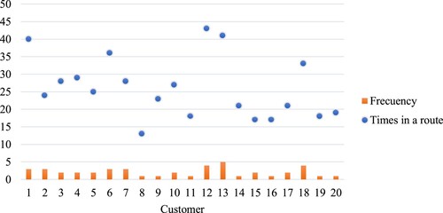
In a similar analysis, in Figure 6 is contrasted the optimal result of the frequency of maintenance visits is contrasted with the number of times each customer appears in a route generated by the proposed method. The customers who appear more in the routes are customers 1, 12, and 13 whose optimal solution (in terms of frequency) is 3, 4, and 5 respectively. On the other hand, the customer with a lower number of times in a route is customer number 8 who has a frequency of 1. In the best solution found, the frequencies generated vary between 1 and 5 and the percentages obtained are 35%, 30%, 20%, 10%, and 5% respectively.

Figure 6. Number of times that each customer is considered in a route and the optimal maintenance frequency.

Bar and dot graph contrasting the frequency and number of times in a route.

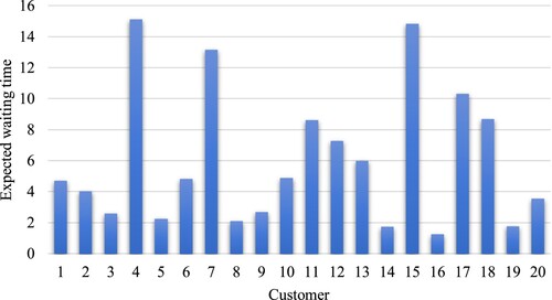
Finally, the expected waiting time before the beginning of the corrective maintenance operation is presented in Figure 7 where for each customer, the solution of the variable $w$ is detailed. It can be analysed that higher waiting times are obtained for customers 4, 7, 15, and 17 and lower waiting time values are obtained for customers 14, 16, and 19.

Figure 7. Expected waiting time before CM.

bar graph of the expected waiting times.

On the other hand, to analyse the impact of a higher instance over the performance of the model, we contrast the results of the previous instance analysed and a bigger one with similar characteristics, but we consider 10 periods of time. Summarising the results obtained, in terms of computational time, the time required for the bigger instance is 10.943 s (which is still a small and reasonable value), the number of iterations increases to 51, and the paths and the patterns to 420 and 712 respectively. In Figure 8 it can be compared the final solution obtained by analysing the period when each customer is visited.

Figure 8. Timer period where each customer is visited (left: 5 time periods, right: 10 time periods).

Two dot graphs contrasting the period when a customer is visited with two different time periods.

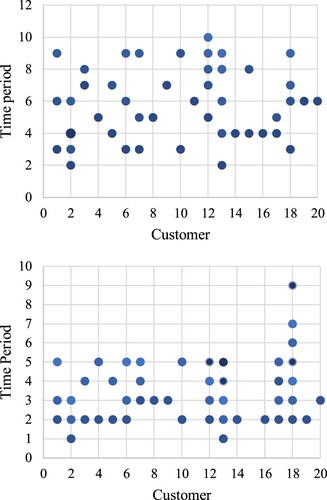
It can be concluded that the frequency for each customer does not change given that the extension of the time periods with the same number of customers can be understood as an extension of a day (increasing for example the number of shifts in a day, therefore 5 days with 1 shift is extended to 5 days with two shifts).

To analyse the robustness of our proposed method, we have generated simulated data to test the solution over the results of an instance. For the instance with five periods and 20 customers, we have obtained the solution of each customer including their frequency and the arrival time to perform the planned maintenance operation (CM or PM). Figure 9 shows the example of one customer with a frequency of two maintenance operations.

Figure 9. Example of a replication of event simulation of one customer with 5 times periods and a frequency of 2 maintenance operations.

From Figure 9 we can analyse different elements. The planning visits are in periods two and four in the planning horizon. Given a MP-CMR solution, a technician arrives at times $s_1$ and $s_2$. For this replication, the machine does not fail before the time $s_1$, thus the technician performs a PM operation with a time $T_{PM}$. The maintenance cost incurred at this time is just preventive cost, and it is computed as $\frac{C_{PM}}{s_1+T_{PM}}$. After the time $s_1+T_{PM}$, the machine is working and fails in a time $A_1$, then the machine must be waiting for the technician arrives to perform a CM operation with a time $T_{CM}$. For this second visit, the cost is corrective maintenance cost plus waiting time cost and it is computed as $\frac{C_{CM}+w{C}_w}{(s_2+T_{CM}-(s_1+T_{PM})}$. The total cost is the sum of the two costs computed.

We built an event simulation model to analyse the performance of each customer and its results (frequency and times where the operations to be performed are planned). We generated random data for the time to failure according to the probability density function for each customer and follow the explanation presented in Figure 9 where we run 10 replications for each customer. The pseudocode of the simulation is presented in Algorithm 2. We use as input the visit pattern set denoted by ${\text{β}}_{it}$, the frequency of maintenance operations denoted by ${\eta }_i$, and the maintenance execution date denoted by $s_k$ for $k=1,\dots ,{\eta }_i$, for each customer $i\in V_c$. These parameters are the solution of the MP-CMR model. Then, the first step of the simulation is focused on generating random times of failures $f_{ik}$ for each customer $i$ and the k-th maintenance operation according to $k=1,2,..,{\eta }_i$. And we determine for each customer $i$ of the times period of each visit $P_{ik}$. After, the second step consists of contrasting the time visit $P_{ik}$ with the time of failure $T{F}_{ik}$ to determine if there is a PM or CM to calculate the anticipation time $A{T}_{ik}$ or the waiting time $W{T}_{ik}$ respectively. For each iteration, we updated the time of renewal $T{R}_{ik}$ that consist in the time after a PM or CM maintenance operations. In addition, we compute the total average maintenance cost ($AVGCost\left(i\right)$) for each customer $i$ adding the preventive or corrective maintenance costs according to the operation executed.

Table

Algorithm 2. Simulation procedure to evaluate the performance of a solution
1:	Input: the visit pattern set ${\text{β}}_{it}$, frequency of maintenance operations ${\eta }_i$, the maintenance execution date $s_k$ for $k=1,..,{\eta }_i$, for each customer $i\in V_c$
2:	First step // Generate for each customer a vector $f_{ik}$ of k-th random times to failure and generate the times which failures will occur according to the probability distribution functions presented in section 7.1
3:	for all $i\in V_c$, $k\in \left\{1,\dots ,{\eta }_i\right\}$
4:	${\mathit{f}}_{\mathit{i}\mathit{k}}=f_i\left(t\right)$ //random time according to pdf $f_i$ of customer $i$
5:	end for
6:	for all $i\in V_c$
7:	$k=1$
8:	for all $t\in \mathcal{T},$
9:	if ${\text{β}}_{it}=1\mathbf{\text{then}}$
10:	$P_{ik}=s_k$ // Calculate the period time during which each visit will occur
11:	$k=k+1$
12:	end if
13:	end for
14:	end for
15:	End first step
16:	Second step // Compare the pattern visit $P_{ik}$ with $T{F}_{ik}$
17:	for all $i\in V_c$
18:	$T{R}_{i1}=0$
19:	$T{F}_{i1}=f_{i1}$
20:	for all $k\in \left\{1,\dots ,{\eta }_i\right\}$
21:	if $P_{ik}\le T{F}_{ik}$ then
22:	$A{T}_{ik}=T{F}_{ik}-P_{ik}$ //calculate the anticipation time
23:	$T{F}_{i,k+1}=P_{ik}+{T_{PM}}_i+f_{i,k+1}$ //calculate the new time of failure
24:	$AVGCost\left(i\right)+={\displaystyle \frac{C_{PM}}{P_{ik}+T_{P{M}_i}-T{R}_{ik}}}$ //add preventive maintenance cost
25:	$T{R}_{i,k+1}=P_{ik}+{T_{PM}}_i$
26:	Else
27:	$W{T}_{ik}=P_{ik}-T{F}_{ij}$ //calculate the waiting time
28:	$T{F}_{i,k+1}=P_{ik}+{T_{CM}}_i+f_{i,k+1}$ //calculate the new time of failure
29:	$AVGCost\left(i\right)+={\displaystyle \frac{C_{CM}+w{C}_w}{P_{ik}+T_{C{M}_i}-T{R}_{ik}}}$ //add corrective maintenance and waiting time costs
30:	$T{R}_{i,k+1}=P_{ik}+{T_{CM}}_i$
31:	end if
32:	end for
33:	end for
34:	End second step

The summary of results is presented in Table 2. The results present for each customer the average number of PM and CM performed, their corresponding percentages given the frequency, the average of anticipation and waiting times, and finally the maintenance cost over the simulated data, the maintenance cost from the MP-CMR model, and the gap between these two costs. It can be concluded that in seven instances 100% of operations performed corresponds to PM meaning that the customers dońt have to wait because of any CM. Also, it can be concluded that on average the percentage of CM operations performed is 6.6%, thus most operations performed corresponds to PM operations given that the objective function creates a balance between the costs of CM, PM, and waiting times. On the other hand, from the second part of the results, it can be concluded that the average anticipation times are greater than the waiting times given in the first part of the results where for 7 instances the results show that customers must not wait in any scenario, meaning that only PM was performed, for the rest of customers the average waiting times are small compared with the anticipation times which is a good factor for keeping continuously the operation. Finally, it can be concluded that on average the model proposed can achieve a reduction of 11.32% over the MP-CMR costs. From the results of these simulations, for five customers we obtained a positive gap, which means an increment of the simulation cost concerning MP-CMR cost. Given the simulation, in some replications, we get only PM or only CM maintenance or combined PM and CM gave the randomness in the data, thus the cost varies with respect to the MP-CMR, however, for most customers the cost is reduced.

It can be concluded that our proposed method is robust to planning the maintenance operation given the objective function of the maintenance model aims to reduce the failure probability and thus the CM operations and waiting times in case a failure happened before a maintenance operation is performed.

Table 2. Summary of results from event simulation model for each customer $i$.

I	Frequency	Average (PM)	Average (CM)	% PM	% CM	Average anticipation time	Average waiting time	Average of maintenance cost from simulation	MP-CMR cost	Gap (%)
1	3	3	0	100.0%	0.0%	26.3	0	45.87	63.04	−27.24%
2	3	2.8	0.2	93.3%	6.7%	89.8	0.6	50.66	63.16	−19.79%
3	2	2	0	100.0%	0.0%	29.6	0	16.14	17.76	−9.12%
4	2	1.9	0.1	95.0%	5.0%	137.7	3.9	20.55	22.88	−10.20%
5	2	1.9	0.1	95.0%	5.0%	24	0.1	20.34	19.72	3.14%
6	3	2.9	0.1	96.7%	3.3%	24.5	0.1	56.92	76.20	−25.30%
7	3	2.5	0.5	83.3%	16.7%	118	11	59.14	61.76	−4.25%
8	1	0.9	0.1	90.0%	10.0%	13	0.6	8.30	7.84	5.85%
9	1	1	0	100.0%	0.0%	31	0	5.44	5.96	−8.78%
10	2	2	0	100.0%	0.0%	31.1	0	13.41	17.40	−22.92%
11	1	0.9	0.1	90.0%	10.0%	67.7	1.7	10.30	8.96	14.97%
12	4	3.7	0.3	92.5%	7.5%	118.6	3.7	101.23	125.88	−19.58%
13	5	4.6	0.4	92.0%	8.0%	165.4	1.8	107.28	116.64	−8.03%
14	1	1	0	100.0%	0.0%	24.1	0	5.82	8.76	−33.58%
15	2	1.7	0.3	85.0%	15.0%	143.1	7.9	28.94	28.08	3.07%
16	1	0.9	0.1	90.0%	10.0%	12.2	0.5	10.05	13.36	−24.79%
17	2	1.6	0.4	80.0%	20.0%	106.8	7.9	35.12	34.64	1.38%
18	4	3.4	0.6	85.0%	15.0%	129.6	3.8	105.97	121.80	−13.00%
19	1	1	0	100.0%	0.0%	24.9	0	6.43	8.48	−24.18%
20	1	1	0	100.0%	0.0%	23.7	0	6.63	6.92	−4.13%

7.3. Computational performance

Once we have detailed a solution of a specific problem, now we will describe the experimentation performed that allows us to analyse different instances and the performance of the proposed method. Thus, the experimentation performed is composed by 5 technicians who perform the maintenance operations, the number of periods analysed are 5, 10, and 20 and the number of customers is from 10 in steps of 10 until an infeasibility is reached, this infeasibility is because of the number of technicians. These results are detailed in Table 3 which contains the number of customers, the objective function found split into the routing and maintenance costs and their percentage, followed by the computational time in seconds. Finally, the number of paths, the number of patterns, and the number of iterations required are detailed in the three last columns.

Table 3. Results with 5, 10, and 20 time periods.

5 time periods
# of customers	Objective Function	Routing	Maintenance	%Routing	%Maintenance	CPU Time (s)	Paths	Patterns	Iterations
20	1857.64	1019	839	54.85%	45.15%	5.61	219	244	45
10 Time Periods
# of customers	Objective Function	Routing	Maintenance	%Routing	%Maintenance	CPU Time (s)	Paths	Patterns	Iterations
20	1819.44	1033	786	56.78%	43.22%	11.08	420	712	51
30	2879.76	1367	1512.76	47.47%	52.53%	41.29	600	1137	76
40	3410.56	1681	1729.56	49.29%	50.71%	158.451	754	1560	110
50	3779.8	1880	1899.8	49.74%	50.26%	122.725	922	1870	122
60	4596.84	2074	2522.84	45.12%	54.88%	185.632	1200	2342	140
20 Time Periods
# of customers	Objective Function	Routing	Maintenance	%Routing	%Maintenance	CPU Time (s)	Paths	Patterns	Iterations
20	1813.28	1023	790	56.42%	43.58%	187.83	1123	1598	145
30	2854.84	1376	1478.84	48.20%	51.80%	410.71	1505	2596	189
40	3392.4	1692	1700.4	49.88%	50.12%	212.859	1761	3444	191
50	3750.16	1889	1861.16	50.37%	49.63%	277.732	2170	4324	208
60	4525.52	2092	2433.52	46.23%	53.77%	400.67	2654	5649	202
70	5170.16	2463	2707.16	47.64%	52.36%	1037.487	3111	7011	401

From Table 3 only one instance can be solved given the short time periods (5) and the number of technicians available. In terms of computational time, the instance can be solved in around 5 s. In terms of the percentage of the objective function, results show that the major portion of the costs is in the routing costs compared with the maintenance costs. On the other hand, the number of patterns generated is greater that the number of paths.

From the second part of Table 3 (10 customers), the number of solvable instances increases to 60. The percentages related to routing and maintenance costs are balanced, which means that they are almost 50% each one. In terms of the computational time between the first two instances, there are not big differences given that the models are solved in less than one minute. Nevertheless, from the instance of 40 customers, the times increase exponentially but is still a reasonable computational time given that times were less than 3 min. Compared with the instances of 5 time periods, the number of paths, patterns and iterations increases (reflected also in the computational time), where the number of patterns generated is around twice the number of paths.

Finally, in the third part of Table 3, results with 20 time periods are presented when an additional instance can be solved (70 customers) where the balance (in terms of proportion) between the routing and maintenance costs is kept. The computational times increase but it is still reasonable given the complexity of the model (the max time used is less than 18 min). The number of patterns is still around twice the number of paths which is related to the number of iterations that also increases.

On the other hand, in Table 4 we present the results of the contrast between the proposed method and benchmark. To show the comparison we have split the results in five columns, the first one corresponds to the objective function where the routing and the maintenance costs are presented in columns two and three respectively. In the fourth column, the CPU time in seconds is presented and the number of paths and the number of iterations is presented in columns five and six respectively. To analyse the experiments, we have fixed the time periods in 5, 10, and 20, and the number of customers varies from 20 to 70 in steps of 10.

Table 4. Results of Multi-Period Combined Maintenance and Routing model (MP-CMR) and benchmark procedure.

		Objective Function			Routing			Maintenance			CPU Time (s)			Paths			Iterations
Time periods	# of customers	MP-CMR	Benchmark	%Improve	MP-CMR	Benchmark	%Improve	MP-CMR	Benchmark	%Improve	MP-CMR	Benchmark	%Improve	MP-CMR	Benchmark	%Improve	MP-CMR	Benchmark	%Improve
5	20	1857.64	1948.4	−5%	1019	1118	−9%	838.64	830.40	1%	5.61	2.42	132%	219	263	−17%	45	59	−24%
10	20	1819.44	2004.96	−9%	1033	1207	−14%	786.44	797.96	−1%	11.08	5.31	109%	420	579	−27%	51	77	−34%
	30	2879.76	3107.64	−7%	1367	1586	−14%	1512.76	1521.64	−1%	41.29	15.19	172%	600	906	−34%	76	116	−34%
	40	3410.56	3794.88	−10%	1681	2103	−20%	1729.56	1691.88	2%	158.451	39.798	298%	754	1303	−42%	110	157	−30%
	50	3779.8	4175.24	−9%	1880	2283	−18%	1899.8	1892.24	0%	122.725	106.103	16%	922	1846	−50%	122	260	−53%
	60	4596.84	5149.72	−11%	2074	2675	−22%	2522.84	2474.72	2%	185.632	240.945	−23%	1200	2799	−57%	140	369	−62%
20	20	1813.28	2108.2	−14%	1023	1330	−23%	790.28	778.20	2%	187.83	11.55	1526%	1123	1191	−6%	145	75	93%
	30	2854.84	3289.36	−13%	1376	1826	−25%	1478.84	1463.36	1%	410.71	75.94	441%	1505	1896	−21%	189	146	29%
	40	3392.4	4017.16	−16%	1692	2352	−28%	1700.4	1665.16	2%	212.859	76.731	177%	1761	2478	−29%	191	163	17%
	50	3750.16	4698.36	−20%	1889	2809	−33%	1861.16	1889.36	−1%	277.732	186.118	49%	2170	3949	−45%	208	252	−17%
	60	4525.52	5534.72	−18%	2092	3119	−33%	2433.52	2415.72	1%	400.67	548.209	−27%	2654	6505	−59%	202	401	−50%
	70	5170.16	7966.32	−35%	2463	4970	−50%	2707.16	2996.32	−10%	1037.487	698.873	48%	3111	6979	−55%	401	386	4%

From Table 4 it can be concluded that the proposed method outperforms the objective function of the whole instances compared to the benchmark where the greatest improvement is related to the routing costs nevertheless there are some instances that the maintenance costs cańt be improved. Given the instances used, it seems that according to the number of customers and the time periods increases, the percentage of improvement of the total costs also increases. In terms of the computational time, the proposed method requires more computational time in seconds but in two instances the amount of computational time is lower compared to the benchmark.

About the waiting times, the behaviour shows that they are not influenced by the period’s length or the frequency of the maintenance operations. Figure 10(a) presents the average of the waiting time for each customer for the planning horizon of 5, 10, and 20 periods and the number of operations performed for 20 customers, where the value of waiting time varies without influence of the customer, periods length or frequency of the maintenance operations. The results evidence the independently behaviour of these parameters or the routing decision in our solution approach. In terms of the paths generated, the proposed method generates a smaller number of paths and requires less iterations compared to the benchmark proposed.

Figure 10. The average of waiting time for T = 5, 10, and 20 periods with (a) 20 customers, (b) 30 customers, and (c) 40 customers.

Three-line graphs and one dot graph presenting the cumulative waiting times and the frequency of visits respectively for 20, 30, and 40 customers.

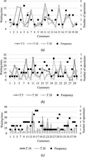
In addition, Figure 10(b) shows the results of waiting times in the case of 30 customers where the same behaviour of 20 customers is found. The frequency or the period’s length is not influenced by the waiting time. The results are similar for the case of 40 customers in Figure 10(c) for 5 and 10 periods.

7.4. Illustrative case study

To illustrate our proposed approach, we applied an example based on a real-world scenario presented (López-Santana et al. 2016). The problem concerns daily operations in an upstream oil and gas company that involves managing a network of interconnected pumping stations that are geographically distributed over a region and subject to unforeseen failures that result in downtime. We assume that the failures are stochastic, and the company has a maintenance department that serves multiple plants (with several pumping stations) scattered over a wide geographical area that covers several towns. The maintenance department performs a variety of activities, including analysis of demand, staff availability, travel times, and maintenance strategies. The department hires technicians with specific skills, for example electrical, mechanical, or instrumentation, with limited working hours per day. They are willing to travel to conduct the maintenance operations.

According with (López-Santana et al. 2016), we consider a set of ten plants geographically distributed, each with a single pumping station. Table 5 shows the travel time between pumping stations and the parameters of the maintenance model for each plant i. There are six technicians with a single set of skills to attend all PM and CM operations. In the real-world case, there is not a central depot for the technicians; indeed, the technicians are located in nodes 1, 2, and 3. We create an artificial depot (denoted by 0) and consider the travel time to nodes 1, 2, and 3 to be zero, and the travel time from the depot to all the other nodes as the maximum travel time among nodes 1, 2, and 3 to the destination node. The parameters of the MM are presented in the next columns of Table 5.

Table 5. Travel time (hours) between pumping stations and maintenance parameters for each plant $i$.

	$j$
$i$	0	1	2	3	4	5	6	7	8	9	10	${C_{PM}}_i$	${C_{CM}}_i$	${C_w}_i$	${T_{PM}}_i$	${T_{CM}}_i$	$f_i\left(t\right)$^1
0	0	0	0	0	3.5	3.5	5	7.5	8.5	9.5	10.5	–	–	–	–	–	–
1		0	1.5	3	3.5	3.5	5	7.5	8.5	9.5	7.5	183	638	15	9	23	$N\left(45,4.091\right)$
2			0	1.5	2	2	3.5	6	7	8	6	121	515	14	5	15	$N\left(54,4.5\right)$
3				0	0.5	1.5	3	5.5	5.5	6.5	10.5	193	425	19	6	17	$W\left(66,3.5\right)$
4					0	1	2.5	5	5	6	10	156	561	14	8	24	$W\left(100,3.5\right)$
5						0	1.5	4	5	6	10	138	567	13	8	17	$W\left(63,3.5\right)$
6							0	2.5	3.5	4.5	8.5	194	498	17	10	15	$N\left(44,4.4\right)$
7								0	1	2	6	163	462	15	9	29	$W\left(84,3.5\right)$
8									0	1	4	100	639	12	9	23	$N\left(78,7.091\right)$
9										0	4	193	580	13	6	23	$N\left(96,8.728\right)$
10											0	105	549	18	10	21	$N\left(75,6.819\right)$

^a By $N\left(\mu ,\sigma \right)$ we denote the normal probability density function with mean $\mu$ and standard deviation $\sigma$; and by $W\left(\lambda ,k\right)$ we denote the Weibull probability density function with scale parameter $\lambda$ and shape parameter $k$.

For planning the operations, we assume eight working hours per day and seven days per week, since the production in the oil and gas industry is uninterrupted. To compare the effect on the schedule of maintenance operations with different horizons, we run two scenarios with one week (7 days) and two weeks (14 days) as the planning horizon.

Table 6 presents the results of the case study with two planning horizons with $\mathcal{T}=7$ and $\mathcal{T}=14$ periods corresponding to one week and two weeks respectively. The objective function provided by the MP-CMR model is less than the value achieved with the benchmark model. The reduction was 37% and 48% for 7 and 14 periods, respectively. In addition, the routing and maintenance have similar behaviour, with fewer values provided by the MP-CMR approach and reductions. Regarding the CPU times, the MP-CMR approach takes more time because it solves the decomposition with two subproblems while the benchmark approach executes just one subproblem. Given the maintenance model is equal for the two models, the frequency of maintenance operations is equal, however, the number of paths and patterns generated by the MP-CMR model is greater than the generated by the benchmark model. Finally, the number of iterations for the case of 7 periods was less by the MP-CMR model against the results of 14 periods, where the iterations increased.

Table 6. Results of Multi-Period Combined Maintenance and Routing model (MP-CMR) and benchmark model on case study with $\mathcal{T}=7$ and $\mathcal{T}=14$.

	7 periods			14 periods
Performance measure	MP-CMR	Benchmark	%Improve	MP-CMR	Benchmark	%Improve
Objective function	253.06	404.70	−37%	573.58	767.46	−25%
Routing	37.50	71.50	−48%	74.50	129.50	−42%
Maintenance	215.56	333.20	−35%	499.08	637.96	−22%
CPU time (s)	1.86	1.17	59%	5.59	1.82	207%
Frequency	14	14	0%	34	34	0%
Paths	155	121	28%	440	210	110%
Patterns	150	20	650%	342	20	1610%
Iterations	32	42	−24%	45	32	41%

Table 7 shows the detailed results of the case study with two planning horizons with $\mathcal{T}=7$ and $\mathcal{T}=14$ periods. We compute the average of maintenance cost for each plant as the total maintenance cost of the plant divided into its frequency of maintenance operations. For the scenario with 7 periods, the average of maintenance cost provided with the MP-CMR model is less than or equal to the value obtained with the benchmark approach for all stations. In the case of 14 periods, the performance was similar for all stations except station 8 with an increment of 2%. Moreover, the frequency of maintenance operations increases from 14 operations in one week to 34 operations in 2 weeks. However, the total average maintenance cost decreased from 135.68 units to 131.57 units. These results suggest that the maintenance planning in general reach a better level despite for some stations the cost increased. Finally, the results are similar to those obtained by (López-Santana et al. 2016), where with a longer planning horizon, the MP-CMR model is still able to achieve low costs better than the benchmark procedure, which lacks the prescriptive power of generate visit patterns.

Table 7. Average of maintenance cost of multi-Period Combined Maintenance and Routing model (MP-CMR) and benchmark model on case study with $\mathcal{T}=7$ and $\mathcal{T}=14$ for each plant $i$.

		7 periods				14 Periods
Plant i		MP-CMR	Benchmark	%Improve		MP-CMR	Benchmark	%Improve
1	2	18.18	18.46	−2%	4	16.96	20.31	−16%
2	2	19.82	27.72	−28%	5	19.88	23.82	−17%
3	1	8.84	22.28	−60%	3	8.92	12.81	−30%
4	1	11.20	11.20	0%	3	11.65	18.84	−38%
5	1	10.92	22.92	−52%	3	10.37	18.13	−43%
6	2	21.02	40.64	−48%	5	20.70	22.94	−10%
7	2	20.86	27.06	−23%	4	20.81	23.26	−11%
8	1	8.12	8.12	0%	2	7.68	7.56	2%
9	1	7.24	12.44	−42%	2	6.88	17.04	−60%
10	1	9.48	28.48	−67%	3	7.72	10.44	−26%
Total	14	135.68	219.32	−38%	34	131.57	175.16	−25%

In summary, the results show that the MP-CMR model gets better results compared with the benchmark model for planning maintenance operations. More importantly, the total, routing, and maintenance costs are better for MP-CMR than the benchmark procedure. The CPU time was increased in the MP-CMR model compared to the benchmark, however, both approaches take less than 6 s. For larger instances, the CPU time could be increased, and it is necessary to evaluate the trade-off between the improvement in the costs versus the computational effort.

8. Conclusions and future work

This work presents a combined multi-period maintenance and routing problem for a set of geographically distributed machines subject to non-deterministic failures. The proposed model is solved through an iterative model based on column generation decomposition where the subproblems generate the paths (or routes) and the visit patterns iteratively. The problem consists of determining a joint routing-maintenance policy for all machines aiming to minimise the routing cost and the total expected maintenance cost composed of preventive and corrective maintenance. We have extended previous work-related by adding the times period in the mathematical model and modifying the connection between the subproblems and we propose an optimisation framework that can be used for solving several classes of maintenance problems.

The experimentation performed allows us to analyse the behaviour of the iterative algorithm contrasting the impact of increasing the number of time periods and the number of customers. Of course, when an instance increases the size the computation time also increases, but in terms of solvability, the number of instances that can be solved is higher.

From the point of view of managerial insights in the industry, our approach led to decision makers to automatise the decisions of maintenance planning and the crew scheduling process involved in a smarter way which contemplates the overall complexity of the process and the uncertainty associated which can avoid being reactive to different events (such as failures) into preventive actions while minimising the overall costs.

From the theoretical point of view, our work can be extended in several directions. First, operators can have specific operations (heterogeneous) splitting the decisions of PM and CM, thus increasing the complexity of decision-making but making the model more adaptable to the reality of the operations. Second, a deterioration factor can be included to analyse the life cycle of machines and the impact on maintenance planning and scheduling. Finally, an indicator of importance given to the CM and the PM can be used to analyse the behaviour of the operation.

In addition, some real-world applications could be explored as future works. In the maintenance planning problem of security services, for example, most of the banks outsource the maintenance of security devices (e.g. video cameras or sensors) in automated teller machines (ATM), where these devices could fail due to damage or vandalism, and then a maintenance operation must be performed to restore them. From the routing point of view, the ATMs are geographically distributed, and the repairmen must travel to perform the maintenance operations in a planning horizon (for instance a week or a month). Likewise, from the maintenance point of view, the failure behaviour could be modelled using a stochastic process to determine the date to planning preventive maintenance operations. Thus, our MP-CMR approach could be applied to obtain maintenance planning for the ATM. Another real-world application arises naturally in utility services, where the service sites are geographically distributed and subjected to unforeseen failures, and the personnel or machinery involved in the maintenance process is a limiting factor. For both areas, because of the prohibitive costs of stopping the operation, the companies need to ensure the highest service levels with appropriate maintenance planning processes.

Acknowledgements

We thank Fair Isaac Corporation (FICO) for providing us with Xpress-MP licenses under the Academic Partner Program subscribed with Universidad Distrital Francisco José de Caldas and Universidad del Rosario. Third author (Carlos Franco) would like to express gratitude to Universidad del Rosario for providing the required funding and support during the research process.

Disclosure statement

No potential conflict of interest was reported by the authors.

Data availability statement

Raw data were generated at ARCOSES Research Group. Derived data supporting the findings of this study are available from the corresponding author ELS on request.

Additional information

Notes on contributors

Eduyn López-Santana

Eduyn López-Santana is assistant professor of Industrial Engineering Department at Universidad Distrital Francisco José de Caldas, Bogotá, Colombia. His research interests include the development and application of optimisation techniques and expert systems to scheduling and engineering design. He is also a member and faculty advisor of student chapter of the Institute of Industrial and Systems Engineers (IISE), and the Colombian Operations Research Association (ASOCIO – Asociación Colombiana de Investigación Operativa).

Germán Méndez

Germán Méndez is professor of operations research of Industrial Engineering Department at Universidad Distrital Francisco José de Caldas, Bogotá, Colombia. His publication list includes around 50 publications, including papers in international academic journals and leading textbooks in Operations Management, Scheduling, Simulation and System Dynamics. His main research interests and results span knowledge-based and expert system to making decision in operations management, mathematical models applied to social and enterprises environments.

Carlos Franco

Carlos Franco is Associate professor at School of Business and Management of Universidad del Rosario, Bogotá, Colombia. His research focuses on the development of mathematical approaches applied to health care logistics and supply chain management.

Appendix A1.

Explanation of the master problem for the routing model

Let $P^k$ be the set of feasible paths for technician $k\in K$ in a period $t\in \mathcal{T}$. Hence, $p\in P^k$ corresponds to an elementary path which can also be described by using the binary values $x_{ijpk}^t$, where $x_{ijpk}^t=1$ if technician $k$ goes directly from vertex $i$ to vertex $j$ on path $p$ on period t, and $x_{ijpk}^t=0$ in otherwise. Any solution $x_{ijk}^t$ to the routing model stated in section 5.1 can be written as a non-negative convex combination of a finite number of elementary paths as follows: (44) $\begin{array}{rl}& x_{ijk}^t=\sum _{p\in P^k}{x}_{ijpk}^t{z}_{pk}^t\mathrm{\forall }k\in K,\left(i,j\right)\in A,t\in \mathcal{T}\end{array}$(44) (45) $\begin{array}{rl}& \sum _{p\in P^k}{z}_{pk}^t=1\mathrm{\forall }k\in K,t\in \mathcal{T}\end{array}$(45) (46) $\begin{array}{rl}& z_{pk}^t\in \left\{0,1\right\}\mathrm{\forall }k\in K,p\in P^k,t\in \mathcal{T}\end{array}$(46) where $z_{pk}^t$ take the value of 1 if a path $p$ is used by one technician $k$ on period $t$ and take the value of $0$ in otherwise. Using $x_{ijpk}^t$ we can define the cost of a path $p$ on period $t$ as $c_{pk}^t$, and the number of times a customer $i$ is visited by technician $k$ on path $p$ on period t as ${\alpha }_{ipk}^t$, and both are computed as follows: (47) $\begin{array}{rl}{c}_{pk}^t& =\sum _{\left(i,j\right)\in A}{c}_{ij}{x}_{ijpk}^t\mathrm{\forall }k\in K,p\in P^k,t\in \mathcal{T}\end{array}$(47) (48) $\begin{array}{rl}{\alpha }_{ipk}^t& =\sum _{j\in V_{C}U\left\{N+1\right\}}{x}_{ijpk}^t\mathrm{\forall }k\in K,i\in V_C,p\in P^k,t\in \mathcal{T}\end{array}$(48) The total routing cost is given by: (49) $\begin{array}{rl}& \sum _{t\in \mathcal{T}}\sum _{k\in K}\sum _{\left(i,j\right)\in A}{c}_{ij}{x}_{ijk}^t\\ & =\sum _{t\in \mathcal{T}}\sum _{k\in K}\sum _{\left(i,j\right)\in A}\left[\sum _{p\in P^k}{c}_{ij}{x}_{ijpk}^t{z}_{pk}^t\right]\\ & =\sum _{t\in \mathcal{T}}\sum _{k\in K}\sum _{p\in P^k}{c}_{pk}^t{z}_{pk}^t\end{array}$(49) Now we can substitute these values into RM formulated in section 5.1 and arrive with the next formulation: (50) $\text{min }\sum _{t\in \mathcal{T}}\sum _{k\in K}\sum _{p\in P^k}{c}_{pk}^t{z}_{pk}^t+\sum _{k\in K}\sum _{i\in V_C}\sum _{r\in R_i}{\phi }_{ir}{y}_{irk}$(50) subject to, (51) $\begin{array}{rl}& \sum _{k\in K}\sum _{r\in R_i}{y}_{irk}=1\mathrm{\forall }i\in V_C\end{array}$(51) (52) $\begin{array}{rl}& \sum _{k\in K}\sum _{p\in P^k}{\alpha }_{ipk}^t{z}_{pk}^t=\sum _{k\in K}\sum _{r\in R_i}{\text{β}}_{irt}{y}_{irk}\mathrm{\forall }i\in V_C,t\in \mathcal{T}\end{array}$(52) (53) $\begin{array}{rl}& \sum _{p\in P^k}{z}_{pk}^t=1\mathrm{\forall }k\in K,t\in \mathcal{T}\end{array}$(53) (54) $\begin{array}{rl}& z_{pk}^t\in \left\{0,1\right\}\mathrm{\forall }p\in P^k,t\in \mathcal{T},k\in K\end{array}$(54) (55) $\begin{array}{rl}& y_{irk}\in \left\{0,1\right\}\mathrm{\forall }i\in V_C,r\in R_i,k\in K\end{array}$(55)

For each machine $i\in V_C$, variables $y_{irk}$ takes the value of 1 whether visit combination $r\in R_i$ is chosen for customer $i$ and technicians $k$, and take the value of 0 in otherwise. The cover constraints (51) guarantee that one visit period combination is selected per machine, constraints (52) link the routes and the visit combinations, and finally, the constraints (53) enforce that one route is selected for each technician $k$ on period $t$.

The set of all feasible routes, which is exponentially large, is denoted by $P$ in the usual case of a single depot and a homogeneous set of technicians with the same initial conditions for all technicians, all $P^k$ are identical, that is, $P=P^k,k\in K$. (56) $\sum _{k\in K}{z}_{pk}^t=z_p^t$(56) where $z_p^t$ is 1 if a path $p$ is used or 0 in otherwise and variable $y_{ir}$ is $1$ if pattern $r\in R_i$ is assigned to machine $i\in V_M$ or $0$ in otherwise. Then, we compute $c_p^t$, $a_{ip}^t$ and $y_{ir}$ as follows: (57) $\begin{array}{rl}& c_p^t=\sum _{\left(i,j\right)\in A}{c}_{ij}{x}_{ijp}^t\mathrm{\forall }p\in P,t\in T\end{array}$(57) (58) $\begin{array}{rl}& {\alpha }_{ip}^t=\sum _{j\in NU\left\{n+1\right\}}{x}_{ijp}^t\mathrm{\forall }i\in N,p\in P,t\in T\end{array}$(58) (59) $\begin{array}{rl}& \sum _{k\in K}{y}_{irk}=y_{ir}\mathrm{\forall }i\in V_M,r\in R_i\end{array}$(59)

Given the set of technicians are homogenous, we omit the index k for the vehicles, and $x_{ijp}^t$ takes the value of $1$ if a technician goes directly from vertex $i$ to vertex $j$ on path $p$ on period t, and $0$ in otherwise, and $c_p^t$ define the cost of a path $p$ on period $t$, and ${\alpha }_{ip}^t$ is the number of times a customer $i$ is visited on path $p$ and period t. Then, the resulting model given below is the classical set partitioning formulation: (60) $Min\sum _{t\in T}\sum _{p\in P}{c}_p^t{z}_p^t+\sum _{r\in R}\sum _{i\in V_M}{\phi }_{ir}{y}_{ir}$(60) Subject to, (61) $\begin{array}{rl}& \sum _{r\in R_i}{y}_{ir}=1\mathrm{\forall }i\in V_M\end{array}$(61) (62) $\begin{array}{rl}& \sum _{p\in P}{\alpha }_{ip}^t{z}_p^t-\sum _{r\in R_i}{\text{β}}_{irt}{y}_{ir}=0\mathrm{\forall }i\in V_M,t\in T\end{array}$(62) (63) $\begin{array}{rl}& \sum _{p\in P}{z}_p^t=m\mathrm{\forall }t\in T\end{array}$(63) (64) $\begin{array}{rl}& z_p^t\in \left\{0,1\right\}\mathrm{\forall }p\in P,t\in T\end{array}$(64) (65) $\begin{array}{rl}& y_{ir}\in \left\{0,1\right\}\mathrm{\forall }i\in V_M,r\in R_i\end{array}$(65)

References

- Ade, C., D. Ouelhadj, D. Jones, M. Stålhane, and I. Bakken. 2017. “Optimisation of Maintenance Routing and Scheduling for Offshore Wind Farms.” European Journal of Operational Research 256 (1): 76–89. doi:10.1016/j.ejor.2016.05.059.
- Adjoul, O., K. Benfriha, C. El Zant, and A. Aoussat. 2021. “Algorithmic Strategy for Simultaneous Optimization of Design and Maintenance of Multi-Component Industrial Systems.” Reliability Engineering and System Safety 208: 107364. doi:10.1016/j.ress.2020.107364.
- Ahmed, M. Ben, F. Zeghal Mansour, and M. Haouari. 2018. “Robust Integrated Maintenance Aircraft Routing and Crew Pairing.”. doi:10.1016/j.jairtraman.2018.07.007.
- Briš, R., P. Byczanski, R. Goňo, and S. Rusek. 2017. “Discrete Maintenance Optimization of Complex Multi-Component Systems.” Reliability Engineering & System Safety 168: 80–89. doi:10.1016/j.ress.2017.04.008.
- Choi, E., and D. W. Tcha. 2007. “A Column Generation Approach to the Heterogeneous Fleet Vehicle Routing Problem.” Computers and Operations Research 34 (7): 2080–2095. doi:10.1016/j.cor.2005.08.002.
- Desaulniers, G., J. Desrosiers, and M. M. Solomon. 2005. Column Generation, edited by G. Desaulniers, J. Desrosiers, and M. M. Solomon. Yu: Springer US. doi:10.1007/b135457.
- Elsido, C., E. Martelli, and I. E. Grossmann. 2021. “Multiperiod Optimization of Heat Exchanger Networks with Integrated Thermodynamic Cycles and Thermal Storages.” Computers & Chemical Engineering 149: 107293. doi:10.1016/j.compchemeng.2021.107293.
- Eltoukhy, A. E. E., Z. X. Wang, F. T. S. Chan, and S. H. Chung. 2018. “Joint Optimization Using a Leader–Follower Stackelberg Game for Coordinated Configuration of Stochastic Operational Aircraft Maintenance Routing and Maintenance Staffing.” Computers & Industrial Engineering 125: 46–68. doi:10.1016/j.cie.2018.08.012
- Eltoukhy, A. E. E., Z. X. Wang, F. T. S. Chan, and X. Fu. 2019. “Data Analytics in Managing Aircraft Routing and Maintenance Staffing with Price Competition by a Stackelberg-Nash Game Model.” Transportation Research Part E: Logistics and Transportation Review 122: 143–168. doi:10.1016/j.tre.2018.12.002.
- Faddoul, R., W. Raphael, and A. Chateauneuf. 2018. “Maintenance Optimization of Series Systems Subject to Reliability Constraints.” Reliability Engineering and System Safety 180: 179–188. doi:10.1016/j.ress.2018.07.016
- Fontecha, J. E., O. O. Guaje, D. Duque, R. Akhavan-Tabatabaei, J. P. Rodríguez, and A. L. Medaglia. 2020. “Combined Maintenance and Routing Optimization for Large-Scale Sewage Cleaning.” Annals of Operations Research 286 (1–2): 441–474. doi:10.1007/s10479-019-03342-8.
- Foong, W. K., A. R. Simpson, H. R. Maier, and S. Stolp. 2008. “Ant Colony Optimization for Power Plant Maintenance Scheduling Optimization—A Five-Station Hydropower System.” Annals of Operations Research 159 (1): 433–450. doi:10.1007/s10479-007-0277-y.
- Francis, P. M., K. R. Smilowitz, and M. Tzur. 2008. “The Period Vehicle Routing Problem and its Extensions.” In The Vehicle Routing Problem (Vol. 43), edited by B. Golden, S. Raghavan, and E. Wasil, 73–102. Springer US. doi:10.1007/978-0-387-77778-8_4.
- Gopalakrishnan, M., M. Subramaniyan, and A. Skoogh. 2020. “Data-driven Machine Criticality Assessment-Maintenance Decision Support for Increased Productivity.” Production Planning & Control The Management of Operations, 1–19. doi:10.1080/09537287.2020.1817601.
- Grigoriev, A., J. Van de Klundert, and F. C. R. Spieksma. 2006. “Modeling and Solving the Periodic Maintenance Problem.” European Journal of Operational Research 172 (3): 783–797. doi:10.1016/j.ejor.2004.11.013.
- Hajej, Z., and N. Rezg. 2020. “An Optimal Integrated lot Sizing and Maintenance Strategy for Multi-Machines System with Energy Consumption.” International Journal of Production Research 58 (14): 4450–4470. doi:10.1080/00207543.2019.1654630.
- Hajej, Z., N. Rezg, and A. Gharbi. 2018. “Quality Issue in Forecasting Problem of Production and Maintenance Policy for Production Unit.” International Journal of Production Research 56 (18): 6147–6163. doi:10.1080/00207543.2018.1478150.
- Hajej, Z., N. Rezg, and A. Gharbi. 2020. “Maintenance on Leasing Sales Strategies for Manufacturing/Remanufacturing System with Increasing Failure Rate and Carbon Emission.” International Journal of Production Research 58 (21): 6616–6637. doi:10.1080/00207543.2019.1683254.
- Han, Y., X. Zhen, and Y. Huang. 2022. “Multi-objective Optimization for Preventive Maintenance of Offshore Safety Critical Equipment Integrating Dynamic Risk and Maintenance Cost.” Ocean Engineering 245: 110557. doi:10.1016/j.oceaneng.2022.110557.
- IBM. 2022. Maintenance Management Software Features. https://www.ibm.com/uk-en/business-operations/maintenance-management?utm_content=SRCWW%26p1=Search%26p4=43700073482957102%26p5=p%26gclid=Cj0KCQiA7bucBhCeARIsAIOwr-_9WwwkVv8sSpNWDQ3UHqs5iSREAbxj2mp4bTTYTb9JdlfNM-KF-qwaAkv5EALw_wcB%26gclsrc=aw.ds.
- Irawan, C. A., D. Ouelhadj, D. Jones, M. Stålhane, and I. B. Sperstad. 2017. “Optimisation of Maintenance Routing and Scheduling for Offshore Wind Farms.” European Journal of Operational Research 256 (1): 76–89. doi:10.1016/J.EJOR.2016.05.059.
- Jardine, A. K. S., and A. H. C. Tsang. 2005. “Component Replacement Decisions.” In Maintenance, Replacement, and Reliability, 27–89. Nu: CRC Press, Taylor & Francis Group.
- Jbili, S., A. Chelbi, M. Radhoui, and M. Kessentini. 2018. “Integrated Strategy of Vehicle Routing and Maintenance.” Reliability Engineering & System Safety 170: 202–214. doi:10.1016/j.ress.2017.09.030.
- Kek, A. G. H., R. L. Cheu, and Q. Meng. 2008. “Distance-Constrained Capacitated Vehicle Routing Problems with Flexible Assignment of Start and End Depots.” Mathematical and Computer Modelling 47 (1–2): 140–152. doi:10.1016/j.mcm.2007.02.007.
- Khatab, A., C. Diallo, U. Venkatadri, Z. Liu, and E.-H. Aghezzaf. 2018. “Optimization of the Joint Selective Maintenance and Repairperson Assignment Problem Under Imperfect Maintenance.” Computers & Industrial Engineering 125: 413–422. doi:10.1016/j.cie.2018.09.012.
- Koochaki, J., J. A. C. Bokhorst, H. Wortmann, and W. Klingenberg. 2012. The Influence of Condition-Based Maintenance On Workforce Planning and Maintenance Scheduling The Influence of Condition-Based Maintenance on Workforce Planning and Maintenance Scheduling. doi:10.1080/00207543.2012.737944.
- López-Santana, E., R. Akhavan-Tabatabaei, L. Dieulle, N. Labadie, and A. L. Medaglia. 2016. “On the Combined Maintenance and Routing Optimization Problem.” Reliability Engineering & System Safety 145: 199–214. doi:10.1016/j.ress.2015.09.016.
- López-Santana, E., J. Romero Carvajal, and J. de. 2015. “A Hybrid Column Generation and Clustering Approach to the School bus Routing Problem with Time Windows.” Ingeniería 20 (1): 111–127. doi:10.14483/udistrital.jour.reving.2015.1.a07.
- Lugtigheid, D., A. Banjevic, and A. K. S. Jardine. 2004. “Modelling Repairable System Reliability with Explanatory Variables and Repair and Maintenance Actions.” IMA Journal of Management Mathematics 15 (2): 89–110. doi:10.1093/imaman/15.2.89.
- Martinod, R. M., O. Bistorin, L. F. Castañeda, and N. Rezg. 2018. “Maintenance Policy Optimisation for Multi-Component Systems Considering Degradation of Components and Imperfect Maintenance Actions.” Computers & Industrial Engineering 124: 100–112. doi:10.1016/j.cie.2018.07.019
- Nemhauser, G. 2012. “Column Generation for Linear and Integer Programming.” Optimization Stories I: 65–73. http://www.emis.ams.org/journals/DMJDMV/vol-ismp/21_nemhauser-george-colgen.pdf.
- Nguyen, H. S. H., P. Do, H.-C. Vu, and B. Iung. 2019. “Dynamic Maintenance Grouping and Routing for Geographically Dispersed Production Systems.” Reliability Engineering & System Safety 185: 392–404. doi:10.1016/j.ress.2018.12.031.
- Ome, J., C. Zhang, Y. Gao, L. Yang, U. Kumar, and Z. Gao. 2018. ARTICLE IN PRESS Integrated Optimization of Train Scheduling and Maintenance Planning on High-Speed Railway Corridors.”. doi:10.1016/j.omega.2018.08.005.
- Remy, E., F. Corset, S. Despréaux, L. Doyen, and O. Gaudoin. 2013. “An Example of Integrated Approach to Technical and Economic Optimization of Maintenance.” Reliability Engineering and System Safety 116: 8–19. doi:10.1016/j.ress.2013.02.001.
- A review on maintenance optimization. 2019. European Journal of Operational Research 285 (3): 805–824.
- Rodriguez, S., D. Correa, and E. López-Santana. 2015. “An Alternative Iterative Method to Periodic Vehicle Routing Problem.” In IIE Annual Conference and Expo 2015, edited by S. Cetinkaya, and J. K. Ryan, 2001–2010.
- Ross, S. 2006. Introduction to Probability Models. 9th ed. Academic Press. http://www.amazon.com/dp/0125980620.
- Ruparathna, R., K. Hewage, and R. Sadiq. 2018. “Multi-period Maintenance Planning for Public Buildings: A Risk Based Approach for Climate Conscious Operation.” Journal of Cleaner Production 170 (1): 1338–1353. doi:10.1016/j.jclepro.2017.09.178.
- Samal, N. K., and D. K. Pratihar. 2015. “Joint Optimization of Preventive Maintenance and Spare Parts Inventory Using Genetic Algorithms and Particle Swarm Optimization Algorithm.” International Journal of System Assurance Engineering and Management 6 (3): 248–258. doi:10.1007/s13198-015-0349-3.
- Solomon, M. M. 1987. “Algorithms for the Vehicle Routing and Scheduling Problems with Time Window Constraints.” Operations Research 35 (2): 254–265. doi:10.1287/opre.35.2.254.
- Toth, P., and D. Vigo. 2002. “The Vehicle Routing Problem.” In Optimization 9: SIAM. doi:10.1137/1.9780898718515.
- Van Horenbeek, A., L. Pintelon, and P. Muchiri. 2010. “Maintenance Optimization Models and Criteria.” International Journal of System Assurance Engineering and Management 1 (3): 189–200. doi:10.1007/s13198-011-0045-x.
- Vassiliadis, C. G., J. Arvela, E. N. Pistikopoulos, and L. G. Papageorgiou. 2000. “Planning and Maintenance Optimization for Multipurpose Plants.” Computer Aided Chemical Engineering 8 (C): 1105–1110. doi:10.1016/S1570-7946(00)80186-8.
- Wakiru, J. M., L. Pintelon, P. Muchiri, and P. Chemweno. 2021. “Integrated Maintenance Policies for Performance Improvement of a Multi-Unit Repairable, One Product Manufacturing System.” Production Planning and Control 32 (5): 347–367. doi:10.1080/09537287.2020.1736684.
- Zhang, L., X. Chen, A. Khatab, and Y. An. 2022. “Optimizing Imperfect Preventive Maintenance in Multi-Component Repairable Systems Under s-Dependent Competing Risks.” Reliability Engineering & System Safety 219: 108177. doi:10.1016/j.ress.2021.108177.
- Zhou, X., & Shi, K. (2019). Capacity Failure Rate Based Opportunistic Maintenance Modeling for Series-Parallel Multi-Station Manufacturing Systems. Reliability Engineering & System Safety, 181, 46–53. doi:10.1016/j.ress.2018.09.007