Intermittent demand, inventory obsolescence, and temporal aggregation forecasts

ABSTRACT

Forecasting for intermittent demand is considered a difficult task and becomes even more challenging in the presence of obsolescence. Traditionally the problem has been dealt with modifications in the conventional parametric methods such as Croston. However, these methods are generally applied at the observed frequency, ignoring any additional information, such as trend that becomes prominent at higher levels of aggregation. We evaluate established Temporal Aggregation (TA) methods: ADIDA, Forecast Combination, and Temporal Hierarchies in the said context. We further employ restricted least-squares estimation and propose two new combination approaches tailored to decreasing demand scenarios. Finally, we test our propositions on both simulated and real datasets. Our empirical findings support the use of variable forecast combination weights to improve TA’s performance in intermittent demand items with a risk of obsolescence.

KEYWORDS:

• Intermittent demand
• decreasing demand
• obsolescence
• temporal aggregation
• temporal hierarchy
• forecast combination

1. Introduction

Intermittent demand remains a typical concern across various industrial sectors, particularly spare parts (Syntetos, Lengu, and Babai 2013). However, the phenomenon has also been extensively studied in several other contexts, such as retail (e.g. Sillanpää and Liesiö 2018), food and pharmaceutical (e.g. Balugani et al. 2019), etc. Parametric methods such as Croston (1972) (CR) and its variants (e.g. Syntetos and Boylan approximation (SBA) (Syntetos and Boylan 2005) are generally considered the standard methods in the forecasting of intermittent demand. In addition, the techniques such as Bootstrapping and Machine learning (ML) (e.g. Hasni et al. 2019; Babai, Tsadiras, and Papadopoulos 2020; Jiang, Huang, and Liu 2020) have also been extensively studied in the context of intermittent demand forecasting. Nonetheless, the assumption that intermittent demand is deprived of any trend and seasonality remains the common trait of most such studies (Kourentzes and Athanasopoulos 2021).

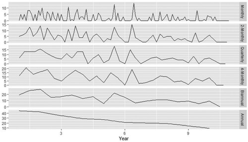
The other important aspect of intermittent demand is that such items are often characterised by an increased risk of obsolescence (Babai et al. 2019). That is generally indicated by a linear or abrupt decrease in the demand occurrence probability (e.g. Prestwich, Tarim, and Rossi 2021) or with increasing instances of zero demand over time (e.g. Teunter, Syntetos, and Babai 2011). In such situations, the conventional parametric methods such as CR and SBA are considered less appropriate, as these methods do not revise the demand estimate in cases of zero demand (Babai, Syntetos, and Teunter 2014). However, based upon the property of constant forecast update, contemporary parametric methods such as Teunter, Syntetos and Babai (TSB) proposed by Teunter, Syntetos, and Babai (2011) and Prestwich, Tarim, and Rossi (2021) are believed to be appropriate for intermittent demand items with a higher risk of obsolescence. Still, most of these forecasting applications usually try to excerpt information from historical observations at the original frequency while ignoring any relevant information at lower frequencies. Although, if analysed closely, intermittent demand series can exhibit a decreasing trend over a long-time. For example, the potential change in a time-series structure at various levels of aggregation for an intermittent demand series is presented with the help of Figure 1. The demand does not display any prominent trend at the original frequency, i.e. monthly, whereas a decreasing trend becomes noticeable at higher time buckets.

Figure 1. Intermittent data series with a prominent decreasing trend at higher aggregation levels.

A figure including six-time series from top to bottom from less aggregated data to more aggregated data and with the bottom series having a clear downward trend.

It becomes evident from the above discussion that it is useful to incorporate information available at the higher aggregation levels into the final forecast at the bottom level. Thus, the use of TA in case of intermittent demand items with an increased risk of obsolescence seems to be a promising idea as:

• TA can help discover specific hidden series characteristics, which may be pronounced across higher aggregation levels. This basic technique helps bring down intermittence, thus allowing for the use of appropriate forecasting methods for fast-moving items (Nikolopoulos et al. 2011). Additionally, the reduced intermittence, at least theoretically, may allow for a more frequent forecast update for conventional parametric methods (e.g. CR, SBA) .¹

• Exploiting several TA levels can help improve the forecasting accuracy of various categories of methods, especially if longer horizons are considered (Petropoulos and Kourentzes 2015; Mircetic et al. 2022).

1.1. Temporal aggregation (TA) and intermittent demand

The TA aggregation technique can primarily be differentiated based on the type of aggregation scheme followed, i.e. overlapping and non-overlapping. In non-overlapping TA, the time series of interest is separated into various fixed time buckets (equal to the considered aggregation level). In overlapping TA, the aggregation window (size equal to the considered aggregation level) keeps moving one step ahead at each period, thus, removing the oldest observation and adding the latest one. The non-overlapping TA is considered more suitable in intermittent demand scenarios (Boylan and Babai 2016); thus, most of such studies consider non-overlapping TA.

Kourentzes, Rostami-Tabar, and Barrow (2017) emphasised that there are two non-overlapping TA techniques in literature: single and multiple TA levels. In intermittent demand, the use of TA can be first attributed to Nikolopoulos et al. (2011), where the authors proposed using an aggregate–disaggregate intermittent demand approach (ADIDA). The methodology relies upon generating a decreased intermittent structure of a demand series at higher TA levels, wherein the forecasts are generated, which are then further disaggregated to the original frequency. The model was further refined by Kourentzes, Petropoulos, and Trapero (2014) using multiple TA levels, and the technique is referred to as the Multiple Aggregation Prediction Algorithm (MAPA). In the strategy, the demand is aggregated at some higher level of aggregation, where an appropriate forecasting model is fitted at each level. In the next step, various components of the time series are combined to get the final forecast. In the intermittent demand context, Petropoulos and Kourentzes (2015) utilised the MAPA framework with certain modifications, wherein the forecasts from different aggregation levels are combined. The authors proved the benefits of such a strategy, using forecasts derived from a single or a combination of different methods.

Lei, Li, and Tan (2016) combined TA with the ‘Fuzzy Markov Chain’ and argued in favour of equal combination weights. Further, Kourentzes, Rostami-Tabar, and Barrow (2017) compared the two approaches (i.e. single and multiple TA levels). The authors argue that identifying an optimal aggregation level is desirable. However, despite the theoretical suboptimality of the multiple TA level technique, the authors propose its use to avoid modelling uncertainty. Thus, the forecast combination (FC) framework proposed by Petropoulos and Kourentzes (2015) is used as one of the TA techniques in the study. In the same context, Fu and Chien (2019) put forward an alternative technique wherein the authors suggested the combination of TA and ML techniques to provide forecasts for the electronic components that are demanded intermittently. For further comprehensive details on the TA approach, the readers are advised to refer to Babai, Boylan, and Rostami-Tabar's (2022) work.

Temporal hierarchy (TH) is the other type of multiple TA level technique similar to the one discussed in the text above. However, the TH technique forces coherence in the forecast at aggregate and disaggregate levels. In other words, the forecast obtained at a higher level of aggregation should be equal to the sum of the forecast at its disaggregated level. With some modification to the original method by Athanasopoulos et al. (2017), the technique with structural scaling (SS) approximation was utilised in the intermittent demand context by Kourentzes and Athanasopoulos (2021). The authors proved its efficacy with the inherent advantage of incorporating information optimally from various levels of aggregation to the final forecast at the bottom level.

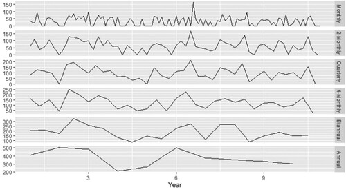
The studies mentioned above have shown the benefits of TA techniques and have even argued for their advantages in the demand series that exhibit trend or seasonality. The studies, however, have not focused on the situations that characterise obsolescence. These combination techniques allow the final forecast to incorporate the additional information present at a higher level of aggregation. Still, the present scheme of assigning weights to the disaggregated forecasts from each level of aggregation warrants further investigation in cases of inventory obsolescence. For example, Figure 2. represents the intermittent demand series that does not display a noticeable trend even at a higher TA level.

Figure 2. Stationary intermittent data series structure at various levels of temporal aggregation.

A figure including six-time series from top to bottom from less aggregated data to less aggregated data and with the bottom series having a clear structure.

Despite the evident difference in the structure of an intermittent demand series for the examples discussed in Figures 1 and 2, the weight combination remains the same for the discussed multiple aggregation level techniques.

Given the above discussion, the present study explores the use of various TA techniques to ascertain their efficacy in the case of an increased obsolescence risk in an intermittent demand context. The study also explores the possibility of assigning varying weights particularly suited to the decreasing demand scenario. The present study proposes two new forecast combination techniques, wherein the optimal weights are obtained with a restricted least square estimation. The efficacy of the proposed models is compared with other TA techniques (ADIDA, FC and TH) by utilising established methods such as CR, SBA, TSB and Exponential Smoothing (ETS) with the help of a simulated and empirical dataset.

The efficacy of the forecasting techniques is generally compared with the help of various forecast accuracy measures. However, the over-emphasis on the results of forecasting accuracy and ignoring the inventory performance aspect can result in misleading conclusions (Kourentzes 2013). Hence, the other aspect of the paper is an inventory performance analysis for the techniques considered in the study.

In summary, the study's main contributions are as follows: It provides a framework for using established forecasting methods with various TA techniques in the cases of increased risk of inventory obsolescence. Further, based upon the ideas of restricted least squared estimations, the study proposes two new forecast combination techniques. The study also compares their forecasting and inventory performance in the said context. The combinations suggested are expected to offer the advantages of both single and multiple TA levels, thus leading to improved forecasting and inventory performance. The comparison of various important aspects of the existing literature with the proposed study is further highlighted with the help of Table 1.

Table 1. Comparison of the proposed study with the existing literature.

Existing research report	Forecasting method employed for the original forecast (Base)	Context	Type of post-processing technique followed.	Inventory Performance Assessment	Additional remark
Nikolopoulos et al. (2011)	Naïve, SBA	Intermittent demand	Forecast from Single aggregation level utilised (ADIDA)	No	The paper empirically demonstrates the usefulness of TA in an intermittent demand context, with a concept of an optimal aggregation level.
Petropoulos and Kourentzes (2015)	Naïve, SES, Moving Average (MA), CR, SBA	Intermittent demand	ADIDA, Forecast combination (FC) from all the considered aggregation levels with equal weightage to the disaggregated forecast from every level	No	The paper proves the efficacy of FC in an intermittent demand context.
Lei, Li, and Tan (2016)	SES	Intermittent demand	FC with simple and weighted mean	No	The paper demonstrates the usefulness of FC with equal weightage to forecasts from all considered levels of aggregation.
Fu and Chien (2019)	MA, CR, SBA, TSB, ML	Intermittent demand	FC with simple and weighted mean	No	The study provides a data-driven framework for combining the forecast obtained from different forecasting methods at each aggregation level.
Kourentzes and Athanasopoulos (2021)	A combination of TSB /ETS (Either ETS or TSB depending upon the intermittence of the demand series (TSB + ETS)	Intermittent demand	TH with SS approximation (equivalent to FC with equal weightage to forecast from every level)	No	Extended the idea of TH in intermittent demand context. This, in turn, can be useful in capturing information (such as trend) that becomes prominent at higher aggregation levels.
Proposed study	CR, SBA, TSB, TSB + ETS	Intermittent demand with a risk of obsolescence	ADIDIA, FC, TH with SS approximation, Proposed FC technique with varying weight combination scheme	Yes	Demonstrates the usefulness of a variable FC weight scheme, particularly in the case of decreasing demand. Furthermore, the proposed technique can prioritise the combination weight scheme according to a particular time series structure.

Overall, the study is structured as follows. First, the considered TA techniques are discussed in detail in the following section. Section 3 contains a discussion regarding the proposed models. Section 4 contains the empirical analysis of the methods discussed in the study, while Section 5 contains the results of the inventory performance analysis. Finally, the study is concluded in section 6, along with the relevant discussion on various implications and future research directions.

2. Temporal aggregation techniques

The present section contains an introduction to the TA techniques such as ADIDA, FC and TH considered in the study.

2.1. Temporal aggregation (TA)

Step 1 aggregation

Let $Y$ be a time series with observation $y_t,t=\left(1,2,\dots ..n\right)$ sampled at the highest observed frequency. Then, the time series can be aggregated in a non-overlapping manner at different aggregation level $sk$ (denoted with $Y^{\left[k\right]}$), with each level containing $n^{\mathrm{\prime }}$ observations such that $n^{\mathrm{\prime }}=\left(1,2,3,\dots n/k\right)$ with $\frac{n}{k}<n$. Where each observation $Y_i^{\left[k\right]}\text{for }i=\left(1,2,3,\dots n/k\right)$ at an aggregation level $k$ can be denoted as $Y_i^{\left[k\right]}=\sum _{t=1+\left(i-1\right)k}^{ik}{y}_t$. However, for specific values of $k$, $\frac{n}{k}$ may not result in integer values; accordingly, $\left[\frac{n}{k}\right]$ observations from the beginning of the series will be dropped from $Y$ (with $n-\left[\frac{n}{k}\right]$ observations remaining) to allow the resulting series to have complete-time buckets.

Step 2 forecasting

The second step consists of forecasting for the series obtained at different levels of aggregation. In this step, generally, any forecasting method suitable for intermittent data or fast-moving scenarios can be used as per the characteristics of the time series at different levels of aggregation.

Step 3 final forecasting

The third step results in the final output, and the process of obtaining the forecast for the original frequency is known as disaggregation. In the original ADIDA technique (Nikolopoulos et al. 2011), the method of disaggregation proposed is intuitive but very effective and can be mathematically represented as follows. (1) ${\hat{y}}_t^{\left[k\right]}=\frac{{\hat{Y}}_i^{\left[k\right]}}{k},\text{for}i=\left[\frac{t}{k}\right]$(1) Where ${\hat{y}}_t^{\left[k\right]}$ represents disaggregated forecast at aggregation level $k$ for time $t$, and $\left[\frac{t}{k}\right]$ represents the integer greater than or equal to the division quotient for $\frac{t}{k}$.

As already emphasised, the ADIDA technique is based upon the idea of an optimal aggregation level, for which the considered forecasting error is minimised. However, there should also be a contemplation on the number of aggregation levels considered, as using an excessively high number will lead to the problem of over-smoothing (Petropoulos and Kourentzes 2015). Apart from the concept of an optimal aggregation level, the combination of forecasts from various methods or at various aggregation levels is considered promising in improving forecasting and inventory performance (e.g. Azevedo and Campos 2016; Wang and Petropoulos 2016). So, the modified framework of MAPA (FC approach) used in the study can be mathematically represented. (2) ${\hat{y}}_t^{\left[C\right]}=\frac{{\hat{y}}_t^{\left[1\right]}}{m}+\frac{{\hat{y}}_t^{\left[2\right]}}{m}+\frac{{\hat{y}}_t^{\left[3\right]}}{m}\dots \dots \frac{{\hat{y}}_t^{,\left[k\right]}}{m}$(2) Where $m$ is the total number of aggregation levels considered.

The final forecast is thus a linear combination of the outputs of various forecasting methods at the different levels of aggregation. For example, if we consider an intermittent demand series observed at the quarterly and aggregated to bi-annual and annual levels. The aggregation scheme thus results in two levels of TA ($m$ = 3). At the same time, the forecast at each level of aggregation is obtained and disaggregated into the highest frequency. In the end, the final forecast obtained at the quarterly level can be written as. (3) ${\hat{y}}_t^C=\frac{{\hat{y}}_t^{\left[1\right]}}{3}+\frac{{\hat{y}}_t^{\left[2\right]}}{3}+\frac{{\hat{y}}_t^{\left[4\right]}}{3}$(3)

Alternatively, the combination can be expressed as follows. (4) ${\hat{y}}_t^C=0.333\ast {\hat{y}}_t^{\left[1\right]}+0.333\ast {\hat{y}}_t^{\left[2\right]}+0.333\ast {\hat{y}}_t^{\left[4\right]}$(4)

2.2. Temporal hierarchies (TH)

The basic concept of TH is similar to the FC approach discussed in the sub-section above. In the TH, similar to the FC, the first step consists of the time series aggregation at various levels of hierarchies. However, the TH approach restricts the number of considered non-overlapping aggregate levels by limiting the value of $12/k$ to an integer. This ensures the seasonality of the aggregated series to be an integer, thus resulting in a relatively less complex forecast combination. In the second step, the forecasts are generated at these aggregation levels (known as ‘base forecast’). Finally, the third and vital stage consists of forecast reconciliation, wherein the ‘base forecast’ is reconciled to the original frequency with the help of various mathematical operations.

In the example considered in section (2.1), the observations at all levels of considered aggregation can be stacked into the following column vector form. (5) $y_i=(Y_i^{\left[4\right]},Y_i^{\left[2\right]},Y_i^{\left[1\right]}{)}^{\mathrm{\prime }}$(5) In the TH approach, a ‘summing matrix $S$’ (Hyndman et al. 2011) forces the original series to be aggregated in a scheme as desired. For example, with $y_i=S\ast b_i$, where $y_i$ is the column vector with all the observations in a hierarchy, $b_i$ signifies the original frequency observations. The summing matrix $s$ ($n\times m$) for the quarterly data can be represented as follows, with $I$ being the identity matrix. $S=\left[\begin{array}{c}\begin{array}{cccc}1& 1& 1& 1\\ 1& 1& 0& 0\\ 0& 0& 1& 1\end{array}\\ I_{4\times 4}\end{array}\right]$

After the aggregation process, the forecast for each aggregation level can be represented in the following column vector form. (6) ${\hat{y}}_i=({\hat{Y}}_i^{\left[4\right]},{\hat{Y}}_i^{\left[2\right]},{\hat{Y}}_i^{\left[1\right]}{)}^{\mathrm{\prime }}$(6)

The observed data in a time series is coherent at all aggregation levels, i.e. it adds precisely across the aggregation levels; however, it is not the case with the base forecast, which needs a reconciliation process, expressed as follows. (7) ${\tilde{y}}_h=SG{\hat{y}}_h$(7)

$S$ helps to sum the forecasts coherently, and $G$ maps the forecast at various aggregations to the bottom level. For example, in the bottom-up approach, the information from the bottom levels is only considered; hence the matrix $G$ is set so that all other aggregation components are assigned a zero coefficient. However, due to ample empirical evidence of the benefits of utilising the information from all the considered aggregation levels, Hyndman et al. (2011) introduced the concept of an optimal approach for utilising the same. Further, Wickramasuriya, Athanasopoulos, and Hyndman (2019) proved that for $G=(S^T{W}_h^{-1}S{)}^{-1}{S}^T{W}_h^{-1}$, the information from all levels of aggregation is used optimally. However, the main issue with the approach is the determination of $W_h$, which can be overcome by using the approximation procedure given by Wickramasuriya, Athanasopoulos, and Hyndman (2019). One such approximation is known as structural scaling, wherein $W_h=\sigma \wedge$, where $\sigma >0,\wedge =dig\left(S1\right)$, where $1$ is the unit matrix of dimension $m$. The reconciled forecast for TH with SS approximation at the quarterly level can be represented as follows. (8) $\begin{array}{rl}{\hat{y}}_t^C& =0.7083\ast Y_{1i}^{\left[1\right]}-0.2916\ast Y_{2i}^{\left[1\right]}-0.04167\ast Y_{3i}^{\left[1\right]}\\ & -0.0417\ast Y_{4i}^{\left[1\right]}+0.2083\ast Y_{1i}^{\left[2\right]}-0.04167\ast Y_{2i}^{\left[2\right]}\\ & +0.0833\ast Y_i^{\left[4\right]},\text{for}i=\left[\frac{t}{k}\right]\end{array}$(8)

The subscript ($1,2,..4$) denotes the specific quarter or half-year; for example, $Y_{2i}^{\left[1\right]}$ denotes the year's second quarter forecast.

The popular methods in intermittent demand contexts such as CR, SBA and TSB provide an identical forecast within a considered aggregation level for the required step ahead; thus, $Y_{1i}^{\left[1\right]}=Y_{2i}^{\left[1\right]}=Y_{3i}^{\left[1\right]}=Y_{4i}^{\left[1\right]}$ and $Y_{1i}^{\left[2\right]}=Y_{2i}^{\left[2\right]}$. Therefore, the combination can be rewritten. (9) $\begin{array}{rl}{\hat{y}}_t^C& =0.3333\ast Y_i^{\left[1\right]}+0.1667\ast Y_i^{\left[2\right]}+0.0833\ast Y_i^{\left[4\right]},\\ & \text{for}i=\left[\frac{t}{k}\right]\end{array}$(9)

It can also be expressed in terms of the desegregated forecast as follows. (10) ${\hat{y}}_t^C=0.333\ast {\hat{y}}_t^{\left[1\right]}+0.333\ast {\hat{y}}_t^{\left[2\right]}+0.333\ast {\hat{y}}_t^{\left[4\right]}$(10)

Even in the case of methods wherein the forecasts are not expected to be identical, the cumulative contribution (from each level of aggregation) remains equal.

Therefore, the approaches such as FC and TH may have many merits. However, it can be expected that information from every level of aggregation will have a different impact on the final forecast at the bottom level, depending on the type of information it contains. On the other hand, the concept of the optimal aggregation level of ADIDA may also be appealing; however, it completely ignores the benefits of forecast combination, if any. As a result, the prospect of assigning weights that can adapt to the changing time series structure is an interesting concept.

3. Proposed techniques

For the TA techniques discussed in the text, the final forecast for the bottom level thus can be expressed by the following mathematical expression. (11) ${\hat{y}}_t^C=\sum _1^k\left({\text{β}}_{k\ast }{\hat{y}}_t^{\left[k\right]}\right)\text{ for }t=1,2\dots ..n$(11) With ${\text{β}}_k$ being the weight coefficient associated with aggregation level $k$. In the case of FC and TH with SS approximation for the same TA levels, ${\text{β}}_1={\text{β}}_2\dots ={\text{β}}_K=1/m$, where m is the total number of aggregation levels. In ADIDA, the $\text{β}$ corresponding to the optimal aggregation level is assigned a weight equal to one, whereas the rest are assigned a weight of zero.

The general equation for the forecast combination at the bottom level of aggregation thus can be considered a regression problem without intercept, which can be formulated mathematically as follows. (12) $y=\text{β}{\hat{y}}^{\left[k\right]}+ϵ$(12) Where $y=[y_1,y_2\dots .y_n{]}^T$, is the $n\times 1$ vector for actual observed demand,${\hat{y}}^{\left[k\right]}$ is the $n\times m$ vector of $n$ disaggregated forecasts for various levels of aggregations (($m=k)$ if all aggregation levels are considered). ${\hat{y}}^{\left[k\right]}=\left[\begin{array}{cccc}{\hat{y}}_1^{\left[1\right]}& {\hat{y}}_1^{\left[2\right]}& \dots .& {\hat{y}}_1^{\left[k\right]}\\ {\hat{y}}_2^{\left[1\right]}& {\hat{y}}_2^{\left[2\right]}& \dots .& {\hat{y}}_2^{\left[k\right]}\\ \dots .& \dots .& \dots .& \dots \\ {\hat{y}}_n^{\left[1\right]}& {\hat{y}}_n^{\left[2\right]}& \dots .& {\hat{y}}_n^{\left[k\right]}\end{array}\right]$

$\text{β}=[{\text{β}}_1,{\text{β}}_2\dots .{\text{β}}_k{]}^T$ is a $m\times 1$ vector of regression coefficients and $ϵ=[{ϵ}_1,{ϵ}_2\dots .{ϵ}_i{]}^T$ is a $n\times 1$ vector of random error terms.

Let ${\text{β}}_A$ be the set of all possible values of vector $\text{β}$, in the case of Ordinary Least squares (OLS) estimators; the objective is to find a vector ${\text{β}}^{ols}=[{{\text{β}}_1}^{ols},{{\text{β}}_2}^{ols}\dots .{{\text{β}}_k}^{ols}{]}^T$ that minimises the sum of squared errors (SSE). (13) $\begin{array}{rl}{S}_{se}\left(\text{β}\right)& =(y-\text{β}{\hat{y}}^{\left[k\right]}{)}^T\left(y-\text{β}{\hat{y}}^{\left[k\right]}\right)\end{array}$(13) (14) $\begin{array}{rl}{\widehat{\text{β}}}^{ols}& =({\hat{y}}^{\left[k\right]T}{\hat{y}}^{\left[k\right]}{)}^{-1}{\hat{y}}^{\left[k\right]T}y\end{array}$(14) However, the direct application of OLS to estimate the weight coefficient for the forecast combination is fraught with two main issues.

1. The elements of ${\widehat{\text{β}}}^{ols}$ can assume negative values that, in turn, may force the ${\hat{y}}_t^C<0$ in the test set, which is undesirable in the present context.

2. The condition related to the sum of coefficients of elements of, i.e. $\sum _1^k{{\widehat{\text{β}}}^{ols}}_k=1$(Hollyman, Petropoulos, and Tipping 2021), may not always be satisfied.

Additionally, the use of OLS for estimating forecast combination weights has been extensively contested in literature (Clemen 1989).

Model 1

The above constraints can be incorporated into the regression model, and the problem can be formulated as a constrained least square problem. (15) $\begin{array}{rl}& mi{n}_{\text{β}}\frac{{\left(y-\text{β}{\hat{y}}^{\left[k\right]}\right)}^T\left(y-\text{β}{\hat{y}}^{\left[k\right]}\right)}{2}\end{array}$(15) (16) $\begin{array}{rl}& s.t.A\text{β}=1\end{array}$(16) (17) $\begin{array}{rl}& \text{β}\ge 0\end{array}$(17)

Where $A=\left[A_{ij}\right]$ is a row matrix with an order of $1\times m$ and with each element $A_{ij}=1$.

The proposed model (referred to as Model 1 for the rest of the study) helps determine the optimal weights within the constraints already defined. The model can force the weights of all disaggregated forecasts except from one aggregation level to zero, or it can even choose equal weights. The approach of selecting the optimal aggregation level will thus become equivalent to the Rostami-Tabar et al. (2013) method, with the optimal aggregation level pertaining to the minimum SSE in the test data set. Model 1 thus can be considered a less restricted TA technique, with ADIDA and the FC as its special cases.

Model 2

The opportunity of determining the weights by allowing the model to choose them with the help of a constrained linear regression is an intuitive and straightforward approach.

In the context of intermittent demand, popular methods such as CR do not revise their forecast in case of zero demand. The intermittence of such a time series decreases with an increasing aggregation level. Thus, leading to a more updated forecast at a higher level of aggregation. Additionally, in situations such as a continuous decrease in demand, the trend information becomes more prominent as we move up the aggregation level. Even for the methods that can incorporate the trend information in the final forecast, the weight coefficients of a higher level of aggregation are intuitively expected to have a more significant impact on the final forecast combination. Therefore, this information can be modelled in Model 1 by assigning a weight that is at least equal to the immediate higher aggregation level; thus, the new model is referred to as Model 2 for the rest of the study.

The mathematical expression for Model 2 is presented as follows. (18) $\begin{array}{rl}& mi{n}_{\text{β}}\frac{{\left(y-\text{β}{\hat{y}}^{\left[k\right]}\right)}^T\left(y-\text{β}{\hat{y}}^{\left[k\right]}\right)}{2}\end{array}$(18) (19) $\begin{array}{rl}& s.t.A\text{β}=1\end{array}$(19) (20) $\begin{array}{rl}& C\text{β}\ge 0\end{array}$(20) (21) $\begin{array}{rl}& \text{β}\ge 0\end{array}$(21)

Where, $C=\left[\begin{array}{ccccccc}-1& 1& 0& \dots & 0& 0& 0\\ 0& -1& 1& \dots & 0& 0& 0\\ 0& 0& 0& \dots & 0& 0& 0\\ 0& 0& 0& \dots & 0& -1& 1\\ 0& 0& 0& \dots & 0& 0& 0\end{array}\right]$

$C=\left[C_{ij}\right]$ matrix with an order of $m\times m$ and two successive elements of a given row $C_{ij+1}=1,and{C}_{ij}=-1$, and all the remaining row elements are zero. Thus, Model 2 is a more restricted form of Model 1, with the weight combination adopted by FC/TH also being a special case of Model 2. However, unlike ADIDA, it is bound to select only the topmost level as the optimal aggregation level.

Both models’ formulations are comparable to the Generalised restricted least-squares (GRLS) (Judge and Takayama 1966) estimation. Firstly, we can derive the first-order necessary conditions for ${\widehat{\text{β}}}^c$ to minimise the formulated GRLS problem. Then, the general form of the Lagrangian function for the minimisation problem for the proposed methods in the study can be given as follows. (22) $\begin{array}{rl}\mathcal{L}& =\frac{{\left(y-\text{β}{\hat{y}}^{\left[k\right]}\right)}^T\left(y-\text{β}{\hat{y}}^{\left[k\right]}\right)}{2}+\gamma \left(A\text{β}-1\right)\\ & +\lambda C\text{β}+\delta \text{β}\end{array}$(22)

With $\gamma ,\lambda$ and $\delta$ being the Lagrange multiplier vectors with $\lambda =\left[{\lambda }_{1j}\right]$ and $\delta =\left[{\delta }_{1j}\right]$ are the row matrix with $m$ elements.

The Karush-Kuhn-Tucker (KKT) optimality conditions that need to be satisfied by vector ${\widehat{\text{β}}}^c$ are represented as follows. (23) $\begin{array}{rl}& \mathrm{\nabla }\mathcal{L}\left[{\widehat{\text{β}}}^c,{\gamma }^{\ast },{\lambda }^{\ast },{\delta }^{\ast }\right]=0\end{array}$(23) (24) $\begin{array}{rl}& A{\widehat{\text{β}}}^c-1=0\end{array}$(24) (25) $\begin{array}{rl}& C{\widehat{\text{β}}}^c\ge 0\end{array}$(25) (26) $\begin{array}{rl}& {\widehat{\text{β}}}^c\ge 0\end{array}$(26) (27) $\begin{array}{rl}& {\gamma }^{\ast }\left(A{\widehat{\text{β}}}^c-1\right)=0\end{array}$(27) (28) $\begin{array}{rl}& {\lambda }^{\ast }{C}_L{\widehat{\text{β}}}^c=0\end{array}$(28) (29) $\begin{array}{rl}& {\delta }^{\ast }{\widehat{\text{β}}}^c=0\end{array}$(29) (30) $\begin{array}{rl}& \lambda \ge 0\end{array}$(30) (31) $\begin{array}{rl}& \delta \ge 0\end{array}$(31)

$\gamma$ is unrestricted in sign

The optimisation problem of the scale similar to the one discussed in the present study can easily be solved with the help of the active set method proposed by Lawson and Hanson (1974). The problem with such algorithms is that they become inefficient in handling large scale GRLS problems. Since the present study is restricted towards demonstrating the effectiveness of an alternative combination technique in special cases of intermittent demand, we restrict ourselves towards the use of the active set method only. For further details on the other techniques that are effective in handling large scale GRLS problems, the readers are advised to refer to the work by Wickramasuriya, Turlach, and Hyndman (2020).

4. Empirical evaluation

The section contains the particulars regarding the experimental arrangement used in the study, such as the details regarding the methods employed, the evaluation metrics, the datasets, and the results of the analysis.

4.1. Forecasting models

In order to evaluate the suitability of existing and proposed TA approaches, the study utilises four forecasting models: CR, SBA, TSB and ETS. CR and SBA are standard methods in intermittent demand forecasting, whereas TSB is considered more suitable for increased risk of obsolescence. However, as already emphasised, the parametric methods do not inherently model trend or seasonality in the data, which can be overcome with the ETS model. The application of ETS thus can help to model a time series into four main components: ‘level, trend, seasonal and an error term’, while their interaction may be additive or multiplicative. For further details on the ETS class of methods, the readers are advised to refer to the research report of Hyndman and Athanasopoulos (2018).

In the present study, the ETS model is expected to better adjust to the decreasing trend scenario, which generally becomes prominent at a higher level of aggregation. However, since the use of ETS has been found to be unreliable with certain intermittent demand datasets (e.g. Ducharme, Agard, and Trépanier 2021), its use for intermittent data may not be an optimal choice. Furthermore, since the study also involves three CR variants, i.e. CR, SBA, and TSB, it is also important to devise a mechanism to choose among these methods. Although certain guidelines exist regarding the use of CR and SBA, there are no clear rules for using other intermittent demand forecasting methods, such as TSB or the forecasting methods, such as ETS (Kourentzes and Athanasopoulos 2021).

Further, Kourentzes (2014) demonstrated that such a classification rule might not be able to outperform simple heuristics solutions with optimised model parameters. Since the present study focusses upon the obsolescence scenario, for which TSB method is considered a suitable choice. The present study thus utilises TSB for intermittent data, and ETS is utilised for continuous data. In order to distinguish between intermittent and continuous demand data, the study utilises the ‘intermittent threshold’ heuristic by Kourentzes and Athanasopoulos (2021). The percentage of periods with zero demand over the total within sample periods is utilised to differentiate between continuous and intermittent demand. In the process, the authors considered four different cutoff limits for categorising demand (10%,20%, 30% and 40%). The authors restrict the cutoff limit to 40% based upon the argument that the parameter estimation becomes challenging for ETS in the presence of increased zero observation in the time series. The authors, through empirical investigation, prove the 10% cutoff limit to be overly restrictive.

Given the above discussion, a cutoff of 40% is to be utilised by the present study. Thus, ETS is utilised for a threshold below 40%; in contrast, for above 40%, the TSB method is utilised. The method thus now involves the use of TSB or ETS at different levels of aggregation depending upon the demand type; thus, it is referred to as TSB + ETS in the rest of the study.

4.2. Model deployment

As the study proposes using restricted least square coefficients as the weights for the TA, the models require the disaggregated forecast related to each level of aggregation. In the case of CR and TSB, the study utilises the tsintermittent package in r (Kourentzes and Petropoulos 2014) to generate the base forecast. In the case of the ETS, the study utilises the forecast package in r (Hyndman and Khandakar 2008) for the same. Further, to estimate the weights for the proposed models, the within-sample observed demand data is regressed upon the within-sample disaggregated forecast(fit) data. Finally, the optimal weight coefficients for each constrained model are obtained with the help of the lsqlincon function available with the pracma package in r (Borchers and Borchers 2021).

4.3. Forecasting performance measures

The forecasting performance measures can be categorised into several categories (e.g. Prestwich et al. 2014); however, two main groups are usually considered: scale-dependent and independent measures. In academic studies related to intermittent demand forecasting, both types of measures have been used to assess the forecasting performance of the contemplated methods. Since the present study plans to conduct statistical analysis on the forecasting accuracy results, the scale-independent measures are favoured. In the process, the study uses three main forecasting performance measures, viz. Scaled Mean Error ($\text{sME}$), Scaled Mean Square Error ($\text{sMSE}$) and Scaled Mean Periods in Stock ($\text{sMPIS}$).

The study uses the mean error to assess the presence of systematic bias (positive or negative) of a particular method. However, due to the requirement of its average over different series, the out-of-sample of respective demand series is scaled with the help of the within-sample mean of observed demand. The scaled error for a particular series ($i)$ over a forecast horizon ($h)$ can be expressed as follows.

Scaled Error(sE) (32) $\text{s}{\text{E}}_{\text{i},\text{h}}=\frac{y_{n+h}-{\hat{y}}_h}{\frac{1}{n}{\sum }_{t=1}^n{y}_t}$(32) Where $n$ is the number of within-sample observations, $y_{n+h}$ is the observed demand at the $h^{th}$ period (out-of-sample), and ${\hat{y}}_h$ is the $h$-step ahead forecast. The scaled Mean Error ($\text{sME}$) values for a particular dataset are obtained as the average of the $\text{sE}$ across all horizons and series of a dataset.

Scaled Squared Error

Apart from the systematic bias of a method, it is also desirable to assess its performance in terms of variance in the forecast obtained. Hence, the study employs the scaled version of mean squared error, where the square of mean of within-sample demand is used as a scaling denominator. The scaled squared error for a particular series ($i)$ over a forecast horizon ($h)$ can be expressed as follows. (33) $\text{sSE}={\left(\frac{y_{n+h}-{\hat{y}}_h}{\frac{1}{n}{\sum }_{t=1}^n{y}_t}\right)}^2$(33) The reported scaled Mean Squared Error ($\text{sMSE}$) values for a particular dataset are obtained as the average of the $\text{sSE}$ across all horizons and series of a dataset.

Scaled Periods in Stock ($\mathit{sPIS}$)

The traditional accuracy measures have often been criticised and considered inadequate in the intermittent demand context (Petropoulos and Kourentzes 2015). For example, the error metrics such as mean Squared and Mean Absolute Errors are focused upon periods with zero demand, thus favouring a biased forecast (Wallström and Segerstedt 2010). Which is of particular concern for highly intermittent demand data. Therefore, Periods in stock ($\text{PIS}$) (Wallström and Segerstedt 2010) acts as an important bias measure (e.g. Petropoulos and Kourentzes 2015). $\text{PIS}$ indicates the number of periods a particular SKU spends in fictitious stock. It not only acts as a measure of the difference between the forecast and the corresponding outcome but combines it with the measure of how long it takes to make the necessary correction. The error measurement is thus augmented with the time dimension (Wallström and Segerstedt 2010). The metric for a series $i$, as defined by Wallström and Segerstedt (2010), can be mathematically defined as follows. (34) $\text{PI}{\text{S}}_i=-\sum _{h=1}^H\sum _{j=1}^h\left(y_{n+j}-{\hat{y}}_j\right)$(34) With $H$ representing the forecasting horizon required, the positive value of the measure is indicative of overstocking, while its negative value signifies understocking.

The $\text{PIS}$ is also a scale-dependent accuracy measure; hence it needs to be made scale-independent to enable its average over a number of time series. The average of within-sample demand further scales PIS to enable its average over a number of demand series.

The scaled Periods in Stock ($\text{sPIS}$) for a score $i$ is given by: (35) $\text{sPI}{\text{S}}_i=\frac{PI{S}_i}{\frac{1}{n}{\sum }_{t=1}^n{y}_t}$(35) The reported scaled Mean Periods in Stock ($\text{sMPIS}$) values for a particular dataset are the mean of the $\text{sPIS}$ across all series of a considered dataset.

4.4. Synthetic data

In order to evaluate the methods discussed in the study, we first use a simulated dataset for the two important cases in the context of intermittent demand. The first one is related to the decreasing demand scenario, and the second is related to the stationary demand; thus, both datasets can help understand the need for a variable weight combination scheme. The study uses the tsintermittent package in r (Kourentzes and Petropoulos 2014) to generate the simulated time series.

In order to generate the data related to decreasing demand scenario, a time series consisting of 120 monthly demand points for a combination of the squared value of the coefficient of variation (CV²) and average inter-demand interval (ADI) is generated. The simulated time series is further aggregated at five levels (bi-monthly, quarterly, four-monthly, bi-annual and annual levels). Finally, the time series with strictly decreasing demand at the annual aggregation level is chosen. If the generated data fails to show such a decreasing trend, the data is regenerated until such a series is found. In order to simulate the data related to stationary demand, the time series is generated without such an arrangement. The descriptive statistics related to the dataset for the decreasing and stationary demand scenarios are listed in Table A1(Appendix A). Table A1 also contains the information regarding the ADI and CV² for the time series at various levels of aggregation. As expected, there is a decrease in the ADI and CV² values with increasing aggregation level for both the datasets. Further, time series decomposition analysis can help understand the strength of data characteristics, including trend and seasonality (Wang, Smith, and Hyndman 2006). Following Makridakis, Wheelwright, and Hyndman (2008), the decomposition of a time series under consideration can be expressed as follows. (36) $y_t=T_t+S_t+R_t$(36) With $T_t$, $S_t$ and $R_t$ being the trend, seasonality and remainder element of the concerned series.

The trend and seasonality strength ($T_S,S_S$) can be expressed as follows (e.g. Hyndman and Athanasopoulos 2018). (37) $\begin{array}{rl}{T}_S& =Max\left(0,1-\frac{Var\left(R_t\right)}{Var\left(T_t+R_t\right)}\right)\end{array}$(37) (38) $\begin{array}{rl}{S}_S& =Max\left(0,1-\frac{Var\left(R_t\right)}{Var\left(S_t+R_t\right)}\right)\end{array}$(38)

A zero strength signifies no trend or seasonality, whereas a value of one signifies perfectly trended or seasonal data. For the simulated dataset (stationary and decreasing), the variation in the trend and seasonality strength with the considered aggregation level is presented herein with the help of Table 2.

Table 2. Time series components strength analysis for synthetic data.

		Demand Scenario
		Decreasing				Stationary
Trend/seasonality Component	Aggregation level	Min	Max	Mean	Median	Min	Max	Mean	Median
Tread Strength	Monthly	0.063	0.420	0.179	0.164	0.033	0.300	0.126	0.129
	Bi-monthly	0.155	0.702	0.344	0.333	0.070	0.495	0.247	0.248
	Quarterly	0.149	0.832	0.474	0.455	0.079	0.688	0.267	0.254
	Four-monthly	0.260	0.854	0.546	0.538	0.099	0.700	0.392	0.395
	Half-yearly	0.423	0.970	0.735	0.734	0.144	0.731	0.402	0.401
	Annual	0.700	0.999	0.944	0.954	0.216	0.824	0.489	0.499
Seasonality Strength	Monthly	0.102	0.498	0.211	0.202	0.089	0.309	0.191	0.189
	Bi-monthly	0.049	0.680	0.235	0.216	0.006	0.392	0.196	0.182
	Quarterly	0.018	0.562	0.227	0.198	0.102	0.401	0.211	0.213
	Four-monthly	0.001	0.645	0.244	0.219	0.164	0.445	0.199	0.184
	Half-yearly	0.001	0.813	0.265	0.210	0.005	0.409	0.191	0.172
	Annual	—–	——	——	—–	—–	—–	—–	——

The analysis of the strength of trend and seasonality components of the simulated datasets provides valuable insight into the context of the present study. Since the time series in both datasets are chosen so that, as expected, the data becomes highly trended with increasing aggregation level for decreasing demand dataset. In contrast, the increase experienced for the stationary demand dataset is not so pronounced. However, not much can be inferred from the seasonality strength for both datasets as they are comparable and do not change appreciably across the datasets.

4.4.1. Results of synthetic data

The present study utilises the last 12 months of the data as test data for the simulated dataset with two forecast horizons (1 and 6 steps ahead), and the remaining dataset serves as within-sample data. The evaluation is performed with the rolling origin forecast update technique (e.g. Hyndman and Athanasopoulos 2018). First, a forecast is generated, and its respective performance is evaluated, while the forecast origin is rolled ahead to expand the training set. Then, the forecasting method is re-estimated, and the process is repeated until all the data in the test set is exhausted. Finally, for the simulated dataset considered in the study, 12 and 7 forecasts are generated for the out-of-sample set.

Table 3 presents the results for the methods considered in the study for a particular forecast horizon for the simulated dataset (least value for a particular technique/accuracy measure highlighted and italicised). With the first column representing the forecasting method employed to obtain the original forecast. Various post-processing techniques used are specified from the fifth column onwards. For example, without aggregation (WA) specifies the results with original methods at a monthly frequency.

Table 3. Forecasting accuracy results for the synthetic dataset (Stationary and decreasing) for CR, SBA, TSB and TSB + ETS methods.

			Accuracy measure
			sMPIS		sME		sMSE
			Dataset Type
Forecast Horizon	Method	TA technique	Stationary	Decreasing	Stationary	Decreasing	Stationary	Decreasing
h = 1	CR	WA	0.862	11.027	−0.074	−0.917	3.362	0.981
		ADIDA	0.756	7.307	−0.062	−0.611	3.381	0.472
		TH	0.712	9.652	−0.058	−0.804	3.323	0.739
		FC	0.714	9.659	−0.058	−0.809	3.324	0.741
		Model 1	0.714	7.142	−0.059	−0.595	3.326	0.439
		Model 2	0.637	7.060	−0.052	−0.587	3.266	0.422
	SBA	WA	0.724	10.526	−0.066	−0.872	3.413	0.882
		ADIDA	0.695	7.348	−0.064	−0.613	3.395	0.483
		TH	0.665	9.548	−0.062	−0.779	3.382	0.697
		FC	0.683	9.412	−0.063	−0.787	3.372	0.700
		Model 1	0.628	7.251	−0.065	−0.574	3.472	0.455
		Model 2	0.728	7.221	−0.075	−0.601	3.449	0.441
	TSB	WA	0.781	9.914	−0.066	−0.826	3.322	0.772
		ADIDA	0.667	7.382	−0.057	−0.615	3.289	0.465
		TH	0.668	9.449	−0.055	−0.768	3.309	0.659
		FC	0.695	9.184	−0.058	−0.765	3.276	0.658
		Model 1	0.550	7.356	−0.047	−0.612	3.310	0.459
		Model 2	0.781	7.353	−0.066	−0.613	3.322	0.435
	TSB + ETS	WA	0.753	9.701	−0.065	−0.814	3.351	0.742
		ADIDA	0.668	1.901	−0.058	−0.202	3.308	0.101
		TH	0.666	4.480	−0.056	−0.401	3.320	0.242
		FC	0.691	4.479	−0.059	−0.402	3.298	0.245
		Model 1	0.620	2.757	−0.075	−0.179	3.611	0.093
		Model 2	0.748	1.746	−0.090	−0.153	3.589	0.078
h = 6	CR	WA	0.614	6.886	−0.083	−0.958	3.530	1.027
		ADIDA	0.573	4.921	−0.074	−0.675	3.499	0.508
		TH	0.556	5.984	−0.070	−0.831	3.423	0.763
		FC	0.564	5.988	−0.071	−0.833	3.454	0.767
		Model 1	0.578	4.836	−0.075	−0.667	3.514	0.457
		Model 2	0.501	4.585	−0.067	−0.628	3.448	0.432
	SBA	WA	0.623	6.651	−0.074	−0.911	3.544	0.928
		ADIDA	0.533	4.497	−0.066	−0.641	3.436	0.504
		TH	0.524	5.742	−0.068	−0.808	3.460	0.719
		FC	0.560	5.978	−0.070	−0.819	3.421	0.722
		Model 1	0.488	4.260	−0.087	−0.606	3.795	0.487
		Model 2	0.610	4.630	−0.111	−0.631	3.789	0.469
	TSB	WA	0.634	6.298	−0.075	−0.876	3.521	0.812
		ADIDA	0.532	4.654	−0.064	−0.654	3.404	0.488
		TH	0.528	5.647	−0.067	−0.759	3.441	0.664
		FC	0.563	5.909	−0.068	−0.772	3.397	0.671
		Model 1	0.438	4.785	−0.055	−0.620	3.497	0.473
		Model 2	0.620	4.754	−0.081	−0.609	3.521	0.466
	TSB + ETS	WA	0.623	5.994	−0.074	−0.841	3.544	0.786
		ADIDA	0.533	1.568	−0.066	−0.211	3.436	0.110
		TH	0.524	3.417	−0.068	−0.369	3.460	0.215
		FC	0.560	3.428	−0.070	−0.367	3.421	0.212
		Model 1	0.488	1.687	−0.087	−0.199	3.795	0.099
		Model 2	0.610	1.607	−0.111	−0.175	3.789	0.085

For the results listed in Table 2, if the results for WA for both the considered forecast horizons and methods are analysed, then the TSB + ETS method is the best-performing model among all the considered ones in case of decreasing demand. In contrast, the results are comparable for all the methods in the case of the stationary demand scenario. Furthermore, the forecasting accuracy results are also on expected lines if analysed based upon the increasing forecast horizon, i.e. generally deteriorating with increasing forecast horizon. Further, the TA techniques improve the forecasting performance for these methods, also referred to as the ‘self-improving mechanism’ (Nikolopoulos et al. 2011). Overall, the models proposed in the study (Model 1 and Model 2) perform as expected in the decreasing demand scenario, with the least mean-variance and bias in the forecast and leading to the least overstocking. In contrast, the TA techniques do not improve forecasting accuracy for stationary demand data.

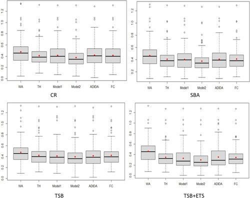
The other important result is related to ADIDA, with the technique showing a significant improvement in forecasting performance compared to FC/TH/WA in the decreasing demand scenario. The results of the ADIDA technique embolden its suitability in the context of decreasing demand scenarios. The other important observation relates to the comparable performance of TH and FC approaches. Thus, concurring with the postulation of their similar forecast combination scheme if the SS technique is used for weights approximation in TH. Further, with Figure 3, the study presents the error distribution (sSE) of the considered methods for the simulated decreasing demand dataset for one-step ahead forecasts (with a black line signifying the median and a red point signifying the mean value) (similar results are obtained for $h=6$ forecasts).

Figure 3. Errors distribution (sSE) for simulated decreasing demand dataset ($h=1$).

A figure including mean error (point in red) and median error (black horizontal line), with the box plots showing the spread of errors (inter-quartile range) and extreme points representing outliers in case of the simulated dataset for one -step ahead forecast obtained by four forecasting methods (CR, SBA, TSB, TSB + ETS) for six different combination techniques.

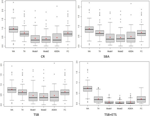
The error distribution confirms the gains in the forecasting accuracy for the proposed models in decreasing datasets, with an apparent distinction in the case of TSB + ETS. The distribution also adds weight to the argument related to the similar forecasting performance of the proposed models and ADIDA. The Friedman test, a non-parametric equivalent of ANOVA, was initially conducted for the $\text{sSE}$ results of all the datasets considered in the study. The Friedman test results indicate at least one technique for which the forecasting accuracy is different in all the datasets except for the stationary demand considered in the study. Subsequently, the Nemenyi test is applied for pairwise comparison to the $\text{sSE}$ results for the decreasing simulated dataset ($h=1$). Figure A1, Figure A2, Figure A3, and Figure A4 (Appendix A) present the statistical test results for the post-hoc Nemenyi test for synthetic data related to decreasing demand scenarios. The statistical analysis results thus establish the improved forecasting accuracy of the models proposed in the study, with Model 2 achieving the minimum rank for all the techniques considered. However, the results fail to establish the statistical significance of the test results among Model 1, Model 2 and ADIDA for most of the methods considered. Nevertheless, the results also establish the comparable forecasting accuracy of the considered TH and FC approach, as discussed in the text earlier. Thus, for decreasing demand scenarios, the favourable results for models proposed in the study and the ADIDA technique support the proposition of a more significant influence of information present at higher aggregation levels.

The results can help better understand the conditions favouring particular techniques if analysed in terms of time series components. For example, in the analysis presented in (Table 2), the trend component becomes highly prominent at the annual aggregation level for the decreasing dataset. Given the above, it can be argued that for the variable FC scheme to have any effect on the forecasting accuracy, there needs to exist a pronounced difference in time series components at different aggregation levels. Thus, if there is a significant change in the strength of time series components, such as a trend with increasing aggregation levels, then the idea of varying the FC scheme seems more beneficial in terms of accuracy improvements. However, the proposed models are expected to show a comparable forecasting accuracy with the existing TA techniques if utilised for time series data that does not display a significant change in its characteristics with changing aggregation levels (stationary dataset in present text).

4.5. Empirical dataset

In the case of the synthetic dataset, there were enough data points to estimate the optimal forecast combination weights for both the proposed models. However, obtaining such a lengthy time series in the context of intermittent demand forecasting in real-life settings is challenging. Therefore, the present study utilises the empirical dataset of 3000 SKUs related to the ‘automotive’ industry. Each demand series comprises 24 months in the dataset, with the respective observation signifying the demand for a particular month. This dataset has been extensively employed in intermittent demand forecasting studies focusing on obsolescence scenarios (e.g. Babai, Syntetos, and Teunter 2014; Sanguri and Mukherjee 2021).

Since the study is focused on the obsolescence scenario; additionally, the simulated stationary dataset results are also indicative of competing forecasting performance for all considered techniques. Accordingly, the study now concentrates only on the decreasing demand scenario in the real dataset. Thus, the complete real dataset is separated into four non-overlapping portions, with strictly decreasing mean demand ($\mu$)in each portion (${\mu }_1>{\mu }_2>{\mu }_3>{\mu }_4$)(e.g. Babai et al. 2019).

This helps identify 147 SKUs, which is later utilised as the empirical dataset in the study. In order to compare the methods discussed in the study, each time series is further aggregated at three levels of aggregation (Bi-monthly, Quarterly and Half-yearly). The dataset thus experiences strictly decreasing demand if observed at a half-yearly level of aggregation. The descriptive statistics for the real decreasing dataset with 147 SKUs in listed in Table A2(Appendix A). Similar to the synthetic dataset there is also a decrease in the ADI and CV² with increasing aggregation level for the real decreasing dataset as well.

Further, based upon the discussion in Section 4.1, the time series characteristics at various levels of aggregation for the considered empirical dataset (147 SKUs with strictly decreasing demand at the bi-annual aggregation level) are presented in Table 4.

Table 4. Time series component strength analysis for the real dataset.

	Demand Scenario
	Decreasing
Aggregation level	Min	Max	Mean	Median
Monthly	0.001	0.843	0.343	0.320
Bi-monthly	0.069	0.958	0.555	0.578
Quarterly	0.230	0.988	0.732	0.776
Half-yearly	0.894	0.999	0.966	0.968
Monthly	0.009	0.864	0.513	0.510
Bi-monthly	0.122	0.917	0.515	0.503
Quarterly	0.039	0.986	0.536	0.550
Half-yearly	0.004	0.996	0.487	0.511

4.5.1. Forecasting accuracy results for empirical data

Since each time series consists of 24 data points, the latest 6 data points are used as the out of -sample portion. Furthermore, the rolling origin method of forecast evaluation with two forecast horizons (1 and 3 steps ahead) is used. At the same time, the other procedures for obtaining the forecast remain similar to as discussed in sections (4.1 and 4.2). Finally, the forecasting accuracy results for the empirical dataset are listed in Table 5 (the least value for a particular technique/accuracy measure highlighted and italicised).

Table 5. Forecasting accuracy results from empirical data.

			Accuracy measure
Forecast Horizon	Method	TA technique	sMPIS	sME	sMSE
h = 1	CR	WA	2.804	−0.467	0.478
		ADIDA	2.410	−0.399	0.417
		TH	2.408	−0.404	0.412
		FC	2.398	−0.400	0.413
		Model 1	2.384	−0.397	0.414
		Model 2	2.240	−0.373	0.388
	SBA	WA	2.762	−0.460	0.468
		ADIDA	2.344	−0.390	0.407
		TH	2.399	−0.401	0.408
		FC	2.380	−0.396	0.409
		Model 1	2.342	−0.390	0.404
		Model 2	2.222	−0.378	0.376
	TSB	WA	2.834	−0.472	0.476
		ADIDA	2.372	−0.396	0.413
		TH	2.485	−0.414	0.422
		FC	2.461	−0.410	0.422
		Model 1	2.396	−0.399	0.410
		Model 2	2.293	−0.382	0.395
	TSB + ETS	WA	2.674	−0.446	0.463
		ADIDA	1.170	−0.195	0.351
		TH	1.818	−0.307	0.346
		FC	1.819	−0.287	0.344
		Model 1	1.201	−0.200	0.327
		Model 2	0.941	−0.155	0.294
h = 3	CR	WA	2.639	−0.496	0.524
		ADIDA	2.298	−0.423	0.420
		TH	2.258	−0.426	0.433
		FC	2.276	−0.428	0.421
		Model 1	2.262	−0.420	0.416
		Model 2	2.121	−0.400	0.392
	SBA	WA	2.641	−0.495	0.522
		ADIDA	2.281	−0.420	0.411
		TH	2.308	−0.428	0.449
		FC	2.310	−0.431	0.418
		Model 1	2.275	−0.417	0.416
		Model 2	2.153	−0.398	0.387
	TSB	WA	2.698	−0.500	0.512
		ADIDA	2.263	−0.409	0.410
		TH	2.359	−0.426	0.431
		FC	2.343	−0.425	0.424
		Model 1	2.288	−0.419	0.411
		Model 2	2.186	−0.402	0.393
	TSB + ETS	WA	2.489	−0.478	0.501
		ADIDA	1.160	−0.216	0.316
		TH	1.715	−0.331	0.347
		FC	1.717	−0.329	0.345
		Model 1	1.193	−0.225	0.301
		Model 2	0.933	−0.174	0.264

The results for the empirical dataset are similar to the one reported in Section (4.4.1), with the considered TA techniques results showing a remarkable improvement compared to the original methods’ results. These results thus further corroborate the findings of literature wherein TA has been shown to improve the forecasting performance of the existing methods; so, the findings can be extended to the cases of decreasing demand. If the overall results are analysed, the proposed models in the study outperform the other considered approach, with Model 2 being the least biased and more accurate for all the methods considered in the study. Similar to section 4.4.1, the forecasting error distribution analysis is further conducted to understand the gains achieved through the proposed models. Figure 4 presents the error distribution for the considered models in the study for $h=1$ forecasts (similar results are obtained for $h=3$ forecasts).

Figure 4. Errors distribution (sSE) for Empirical dataset ($h=1$).

A figure including mean error (point in red) and median error (black horizontal line), with the box-plots showing the spread of errors (inter-quartile range) and extreme points representing outliers in case of the empirical dataset for one -step ahead forecast obtained by four forecasting methods (CR, SBA, TSB, TSB + ETS) for six different combination techniques.

The results of error distribution analysis are less forthcoming than in the case of simulated data; still, they are indicative of distinctively improved forecasting accuracy of the proposed Model 2. This is still important considering the limited data for the optimal forecast combination scheme estimation. If the improvements in the forecasting accuracy for the proposed models are analysed with the help of error distributions of simulated and empirical datasets (Figures 3 and 4). The higher improvements for the simulated dataset can be attributed to sufficient data points that allow the proposed models to estimate the forecast combination weights better.

The results are tested further statistically, with Figure A5, Figure A6, Figure A7 and Figure A8(Appendix A) presenting the post-hoc Nemenyi test for empirical data ($h=1$). Overall, the results for statistical analysis establish the advantages of the TA techniques in the case of decreasing demand scenarios for intermittent demand items. Further, the results also confirm the superior forecasting accuracy of Model 2, as it is the best-performing model with a significant difference in the forecasting accuracy from other considered TA techniques for all the three methods considered in the study. However, in contrast to the results obtained from the synthetic dataset, the forecasting accuracy for Model 1 and ADIDA are similar to the FC/TH technique. Thus, indicating a relationship between the forecasting accuracy of Model 1 with the length of within-sample fit data required to assess the optimal combination/aggregation level. Finally, the results are also significant, as in the literature related to inventory obsolescence, the studies using similar datasets have reported marginal improvements in the forecasting accuracy by using the same methods (e.g. Babai et al. 2019). In contrast, the results obtained in the present study suggest substantial improvements if the mean values of the TA techniques are considered.

6. Inventory performance

Since there is no clarity in the literature regarding the advantage of $PIS$ measure compared to the other inventory performance assessment techniques available. Consequently, a separate inventory performance analysis for the techniques is also performed. The process of obtaining the results of inventory metrics involves choosing an inventory policy. For example, the order-up-to policy (R, S) is the most widely accepted policy for intermittent demand items (Teunter and Sani 2009). The policy involves deciding a review period(R) along with maximum stock position or order-up-to level(S). For the present study, we use a setup similar to that of Teunter and Sani (2009) and Kourentzes (2013), wherein S is expressed as follows. (39) $S={\hat{y}}_{\left(L+R\right)}+K\ast {{\sigma }^F}_{\left(L+R\right)}$(39) Where ${\hat{y}}_{\left(L+R\right)}$ is the forecasted demand over the period $\left(L+R\right)$, with $R$ representing the review period, $L$ denoting the lead time and $K$ is the safety factor corresponding to a ‘target service level’ obtained from the normal distribution for the preferred service level. While ${{\sigma }^F}_{\left(L+R\right)}$ is expressed mathematically as follows. (40) ${{\sigma }^F}_{L+R}=\sqrt{\left(L+R\right)MS{E}_t}$(40) Where $MS{E}_t$ (Smoothed MSE) is the standard error computed with one-step ahead forecasts. $MS{E}_t$ can be expressed with the help of the below-mentioned formula (for further details, please refer to Syntetos and Boylan (2008) and Syntetos et al. (2009)). (41) $MS{E}_t=\left(1-\delta \right)\ast MS{E}_{t-1}+\delta \ast (y_t-{\hat{y}}_t{)}^2$(41) For the present study, we assume $L=1$ and $R=1$; thus, the protection interval is equal to (L + R = 2); accordingly, the forecast horizon for the evaluation is fixed at $h=2$. The study considers four values of target service level (0.8, 0.9, 0.95, and 0.99), for which the relevant values of $K$ are obtained from a standard normal distribution table. While the value for $\delta$ is fixed at 0.2.

For the analysis, the observed demand is deducted from the stock on hand for every period. If the resulting stock (stock on hand + on order) goes below stock level S (updated every period), the difference amount is ordered. The other important aspect is regarding the initialising stock, which is assumed to be equal to the demand in the first test period.

The realised service level corresponds to the probability of not stocking out in a considered cycle, and the corresponding stock holding is measured in the study. The analysis results must be considered very carefully as comparing the techniques based on the service levels alone may not provide an accurate assessment (Kourentzes 2013.) Thus, the efficiency curves provide insight into the amount of stock required by each technique against a target service level. The techniques that retain higher stock may still achieve a higher service level. Thus, the realised service level needs to be analysed with the corresponding stock level. The actual stock holding thus acts as a cost parameter, an essential indicator of a technique’s performance. In order to make the actual stock holding additive for the entire dataset, we scale the values with the mean of positive within sample demand.

The average scaled holding stock (ASH), and average realised service level (ARSL) based upon a target service level (TSL) for the simulated and empirical data considered in the study are presented in Figures 5 and 6, respectively.

Figure 5. Efficiency curves for inventory performance analysis for simulated decreasing dataset ($L=1,R=1$).

A figure including the average realised service level (Y-axis) and average scaled holding stock (X-axis) for the simulated decreasing dataset, with each point depicting the realised service level against the target service level and the lines providing the results for the forecast obtained by four forecasting methods (CR, SBA, TSB, TSB + ETS) for six different combination techniques.

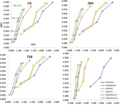
Figure 6. Efficiency curves for inventory performance analysis for the real dataset ($L=1,R=1$).

A figure including the average realised service level (Y-axis) and average scaled holding stock (X-axis) for the real dataset, with each point depicting the realised service level against the target service level and the lines providing the results for the forecast obtained by four forecasting methods (CR, SBA, TSB, TSB + ETS) for six different combination techniques.

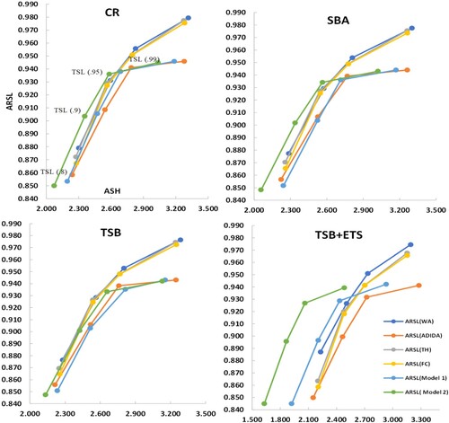
The sME results reported for both the datasets (synthetic and real) for all the considered techniques are negative (moderate to high), indicating overprediction (error = actual demand – forecasted demand). Accordingly, the inventory performance analysis results are on the expected lines as all the considered techniques are able to achieve high service levels for both the datasets. However, the sME values are more negative in the case of the synthetic dataset than in the real dataset. Thus, the higher ARSL values in the case of the synthetic dataset than the real dataset further substantiates the argument regarding overprediction. Since there is not a huge difference in the realised service levels for all the considered techniques. Thus, the main difference among the techniques lies in the ASH, which indicates the amount of stock required to achieve the corresponding service levels. The results of both the datasets considered for inventory performance analysis are similar with the proposed models providing competing realised service levels with a significantly reduced inventory. The WA technique (for CR, SBA, TSB, TSB + ETS) for both datasets provide higher service levels; however, it comes at a substantial increase in stock holding. While the proposed models (Model1and Model 2) provide comparable service levels with substantially reduced stock levels.

If analysed in terms of increasing target service level, the results also show a similar trend for each considered technique and forecasting model. The corresponding stock holding increases with an increase in the target service level. Overall, there is a decrease in the ARSL for the proposed techniques. However, this can be attributed to a substantial decrease in the actual stock holding. Thus, adding weight to the argument regarding the suitability of the proposed techniques in the decreasing demand context.

7. Conclusion, research implications and further research directions

Due to its inherent slow-moving character, intermittent demand items often lead to a higher risk of obsolescence. Several researchers have contributed to the area; however, the models put forward have mainly been the variants of Croston's method that show marginal improvements in forecasting accuracy over their predecessors. Furthermore, the application of such methods is limited to the frequency at which the data is observed. Whereas the additional information available at a higher time bucket is generally ignored. Therefore, the concept of TA, i.e. examining the time series at various levels of aggregations (in terms of time hierarchy), presents itself as a promising option in situations with a higher risk of obsolescence. Thus, the present study applies single (ADIDA) and multiple TA levels (FC and TH) techniques in the said context. The TA techniques have various structural differences; while ADIDA strives to discover an optimal aggregation level, FC and TH depend upon the combination of forecasts.

Further, despite the similarity between FC and TH, the techniques differ in choosing their weight combinations. FC relies upon the mean weight ratio; the TH involves a complex procedure to arrive at the optimal weight combinations. However, the present study proves the equivalence of the forecast combinations obtained from FC and TH (with structural scaling approximation) if methods that provide a constant forecast are used (e.g. CR, TSB). Therefore, though the forecast combination techniques such as FC have proved efficient, the strategy is considered sub-optimal.

Additionally, these forecast combination techniques do not have any provision for varying the combination of the weights based on the time series structure. Hence, the study proposes two new approaches to modify the forecast combination strategy followed by the existing techniques. The study uses two restricted least squared estimations for obtaining a varying weight combination scheme. In Model 1, the study entirely relies upon the data to select the optimal combination/aggregation level scheme. Whereas in the second approach (Model 2), the study designs the scheme of combination dependent upon the postulation that the disaggregated forecast obtained from a higher level of aggregation is expected to have a more significant effect on the final forecast. In order to test the above postulations, the study compares the forecasting performance of proposed models with established TA techniques by using popular forecasting methods such as CR, SBA, TSB and ETS in cases of both simulated and empirical datasets.

In the simulated dataset, two datasets are generated: decreasing and stationary demand. The results of the comparison of the forecasting accuracy are on the expected lines, as the existing TA techniques (ADIDA/FC/TH) lead to improved forecasting performance for the considered methods. Another critical observation pertains to the superior forecasting performance of the ADIDA technique in comparison to FC and TH in the decreasing demand scenario. Overall, the two models proposed in the study show substantial improvements in the forecasting performance for the decreasing demand scenario. While in the case of stationary demand, the results from all the considered techniques are comparable.

The results from the synthetic dataset are encouraging; however, they may be attributed to the presence of substantial data to estimate improved forecast combination weights. Additionally, such lengthy time series in intermittent demand is often an exception. Hence, the efficacy of the proposed models is also compared with the help of an established short empirical intermittent dataset.

The dataset is further filtered to identify the time series that exhibit decreasing demand over a period of time. The results of the empirical dataset also indicate the superior forecasting accuracy of the models proposed in the study. The synthetic and empirical dataset results are further validated statistically, establishing the superior forecasting accuracy of the proposed models in the study in the context of intermittent demand with the risk of obsolescence.

Overall, the study makes important contributions to the theory and practice of applying TA techniques in the context of intermittent demand forecasting, especially in case of an increased risk of obsolescence. Firstly, the study extends the idea of the usefulness of TA techniques in the context of the problem of obsolescence in intermittent-demand items. Additionally, it provides a general framework for their application in the said context. Further, it proposes two robust techniques for selecting an appropriate forecast combination scheme, which depends on the structure of a particular time series. Lastly, the application of the models proposed by the study is not dependent upon using any particular method and can be extended to other suitable methods for intermittent demand items.

The study has important implications for managers, especially when dealing with spare parts inventory in the automobile and heavy machinery sectors. The managers in such areas have to deal with spare parts ordered intermittently that are also prone to a higher risk of obsolescence. In such situations, the managers have the option of only a few methods that can react fast to a decreasing demand scenario. In contrast, the use of TA techniques can immensely improve the forecasting performance of the already established methods. At the same time, its forecasting performance can be further improved with the help of the models proposed in the study. Furthermore, reducing the intermittence at higher aggregation levels also allows the application of methods designed for fast-moving items.

Although the study focuses on an interesting aspect, the study has some limitations; for example, the study considers a simple heuristic for differentiating between intermittent and continuous demand for the application of the ETS or TSB model. The merits of model selection at various TA levels can be examined in terms of the probable avenues of future research. Further, a limited empirical dataset is considered in the study, which restricts the generalisation of the study's results. Thus, the dataset with an even higher frequency or other popular empirical datasets with high intermittence can be considered for future analysis. The other significant extension can be to consider the performance of algorithms suitable for large-scale constrained least square estimate problems to enable a more general application of the proposed models. The proposed models can also be tested in similar situations wherein the time series structure changes considerably with the increasing aggregation levels. For the inventory performance analysis, the assumption of normality may not be valid for the intermittent demand context; thus other assumptions can be further examined.

Disclosure statement

No potential conflict of interest was reported by the author(s).

Data availability statement

The data that support the findings of this study are available from the corresponding author, KN, upon reasonable request.

Additional information

Notes on contributors

Kamal Sanguri

Mr. Kamal Sanguri is an Assistant Professor in School of Management at Graphic Era Hill University, Bhimtal campus. His research interest includes demand forecasting, and inventory management. His research papers have featured in reputed journals such as Journal of Forecasting, Journal of Cleaner production, Computers and Industrial Engineering, Scientometrics and Expert Systems with Applications.

Sabyasachi Patra

Dr. Sabyasachi Patra is an Associate Professor in Operations Management & Decision Sciences at the Indian Institute of Management Kashipur. He received his PhD from Industrial and Management Engineering Department, Indian Institute of Technology Kanpur. His areas of research interests include parametric and non-parametric regression, statistical learning theories and its applications in business data analysis.

Konstantinos Nikolopoulos

Dr. Konstantinos (Kostas) Nikolopoulos is the Professor in Business Information Systems and Analytics at Durham University Business School. Dr. Nikolopoulos studied Electrical and Computer Engineering at the National Technical University of Athens (ΕΜΠ) in his native Greece (D.Eng. 2002, Dipl. Eng. 1997). He further completed the International Teachers Programme (ITP) at Kellogg School of Management at Northwestern University (2011). His research interests are Forecasting, Analytics, Information Systems, and Operations. Dr. Nikolopoulos was Professor of Business Analytics/Decision Sciences at Bangor University for a full decade, and completed three tenures as the College Director of Research (Associate Dean for Research & Impact) for the College of Business, Law, Education, and Social Sciences (2011–2018) in charge of the REF2014 submission for the Business and the Law school. Before that, he was Lecturer and Senior Lecturer in Decision Sciences at the University of Manchester, a Senior Research Associate at Lancaster University and the CTO of the Forecasting and Strategy Unit (www.fsu.gr) in the Electrical and Computer Engineering Department of the National Technical University of Athens (1996–2004). He has also held fixed-term teaching and academic appointments in the Indian School of Business, Korea University, University of the Peloponnese, Hellenic International University, RWTH Aachen, Lille 2, and more recently in Kedge Business School. Professor Nikolopoulos is an Associate Editor of Oxford IMA ‘Journal of Management Mathematics’ and the ‘Supply Chain Forum, an International Journal’ (Taylor & Francis); he is also the Section Editor-In-Chief for the ‘Forecasting in Economics and Management’ section in the MDPI open access journal ‘Forecasting’.

Sushil Punia

Sushil Punia is an Assistant Professor at IIT Kharagpur (India). He holds a Ph.D. degree from IIT Delhi and an M.Tech degree in Industrial Engineering and Management from IIT Kanpur. His areas of interests include operations and supply chain management, forecasting and predictive analytics, and data-driven optimisation with applications in healthcare delivery and urban logistics. His research has been published in research journals like EJOR, IJPR, DSS, CAIE, and others.

Notes

1 Although the conventional parametric methods (e.g., CR, SBA) are designed for intermittent demand data, these methods still update their forecast only in a period with non-zero demand (Teunter, Syntetos, and Babai 2011). However, since TA is expected to reduce the intermittence of such a series at higher aggregation levels, thus the forecast obtained with such methods is expected to be more updated at higher aggregation levels.

Appendix A

Table A1. Descriptive statistics synthetic data.

Scenario	Aggregation Level	Minimum Mean Demand	Average Mean demand	Maximum Mean demand	Minimum ADI	Mean ADI	Max ADI	Minimum CV^2	Mean CV^2	Max CV^2
Decreasing demand	Monthly	1	43.40	145.75	1.47	3.78	7.62	0	1.03	5.22
	Bi-monthly	1.41	49.01	155.46	1.08	2.15	3.84	0.13	0.99	3.63
	Quarterly	2.03	56.88	184.80	1.05	1.66	2.71	0.10	0.93	3.16
	Four monthly	2.50	64.93	208.91	1.00	1.41	2.08	0.17	0.88	2.99
	Half-yearly	3.82	81.99	304.88	1.00	1.18	1.63	0.13	0.76	2.35
	Annual	6.5	136.93	518.3	1.00	1.00	1.00	0.08	0.61	1.69
Stationary demand	Monthly	5.19	64.28	126.01	1.33	2.62	7.4	0.26	0.97	3.04
	Bi-monthly	8.10	84.82	191.38	1.01	1.63	4.00	0.19	0.86	2.53
	Quarterly	10.56	107.66	283.30	1.00	1.32	2.64	0.22	0.77	2.38
	Four monthly	13.50	132.81	376.4	1.00	1.19	2.15	0.17	0.66	1.92
	Half-yearly	20.25	186.71	564.6	1.00	1.07	1.58	0.09	0.54	1.97
	Annual	36.86	359.79	1129.2	1.00	1.09	1.25	0.01	0.31	1.33

Table A2. Descriptive statistics real data (147 SKUs with strictly decreasing demand at Bi-annual level).

Aggregation Level	Minimum Mean Demand	Average Mean demand	Maximum Mean demand	Minimum ADI	Mean ADI	Max ADI	Minimum CV^2	Mean CV^2	Max CV^2
Monthly	1.36	5.84	66.08	1.00	1.22	1.85	0.00	0.47	1.47
Bi-monthly	1.90	10.21	127.66	1.00	1.04	1.33	0.05	0.40	1.64
Quarterly	2.35	14.97	191.50	1.00	1.01	1.14	0.02	0.34	1.10
Half-yearly	4.75	29.54	383.00	1.00	1.00	1.00	0.01	0.24	1.08

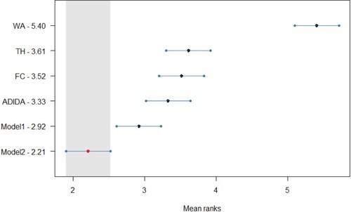
Figure A1. Statistical comparison of forecasting accuracy in case of decreasing demand scenario (Synthetic Dataset) for CR method, Critical distance  = 0.754.

A figure including the point error (in red) and the respective confidence intervals (in blue) for six different methods for CR method for synthetic dataset, from left to right and bottom to top these being Model 2 then Model 1 then ADIDA then FC then TH and then WA.

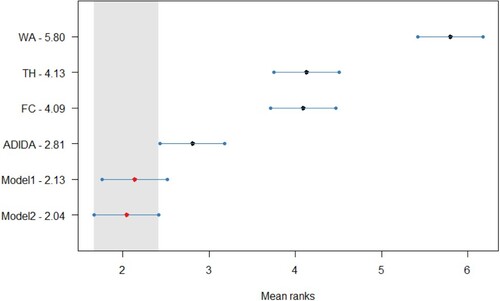
Figure A2. Statistical comparison of forecasting accuracy in case of decreasing demand scenario (Synthetic Dataset) for SBA method, Critical distance  = 0.754.

A figure including the point error (in red) and the respective confidence intervals (in blue) for six different methods for SBA method for synthetic dataset, from left to right and bottom to top these being Model 2 then ADIDA then Model 1 then TH then FC and then WA.

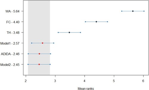
Figure A3. Statistical comparison of forecasting accuracy in case of decreasing demand scenario (Synthetic Dataset) for TSB method, Critical distance  = 0.754.

A figure including the point error (in red) and the respective confidence intervals (in blue) for six different methods for TSB method for synthetic dataset, from left to right and bottom to top these being Model 2 then ADIDA then Model 1 then FC then TH and then WA.

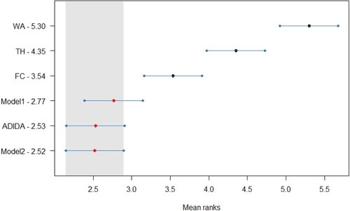
Figure A4. Statistical comparison of forecasting accuracy in case of decreasing demand scenario (Synthetic Dataset) for TSB + ETS method, Critical distance  = 0.754.

A figure including the point error (in red) and the respective confidence intervals (in blue) for six different methods for TSB + ETS method for synthetic dataset, from left to right and bottom to top these being Model 2 then Model 1 then ADIDA then FC then TH and then WA.

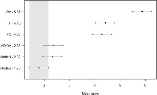
Figure A5. Statistical comparison of forecasting accuracy in case of decreasing demand scenario (Empirical Dataset) for CR method, Critical distance = 0.622.

A figure including the point error (in red) and the respective confidence intervals (in blue) for six different methods for CR method for empirical dataset, from left to right and bottom to top these being Model 2 then ADIDA then Model 1 then FC then TH and then WA.

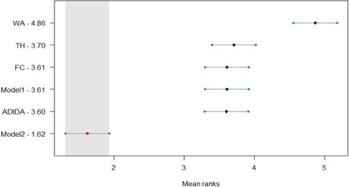
Figure A6. Statistical comparison of forecasting accuracy in case of decreasing demand scenario (Empirical Dataset) for SBA method, Critical distance = 0.622.

A figure including the point error (in red) and the respective confidence intervals (in blue) for six different methods for SBA method for empirical dataset, from left to right and bottom to top these being Model 2 then Model1 then ADIDA then FC then TH and then WA.

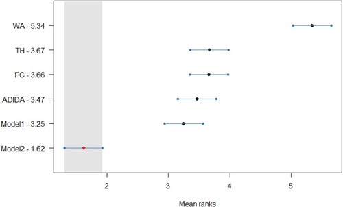
Figure A7. Statistical comparison of forecasting accuracy in case of decreasing demand scenario (Empirical Dataset) for TSB method, Critical distance = 0.622.

A figure including the point error (in red) and the respective confidence intervals (in blue) for six different methods for TSB method for empirical dataset, from left to right and bottom to top these being Model 2 then ADIDA then Model 2 then FC then TH and then WA.

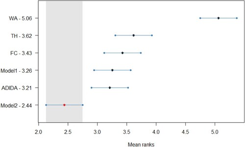
Figure A8. Statistical comparison of forecasting accuracy in case of decreasing demand scenario (Empirical Dataset) for TSB + ETS method, Critical distance = 0.622.

A figure including the point error (in red) and the respective confidence intervals (in blue) for six different methods for TSB + ETS method for empirical dataset, from left to right and bottom to top these being Model 2 then Model1 then ADIDA then FC then TH and then WA.

References

- Athanasopoulos, G., R. J. Hyndman, N. Kourentzes, and F. Petropoulos. 2017. “Forecasting with Temporal Hierarchies.” European Journal of Operational Research 262 (1): 60–74. doi:10.1016/j.ejor.2017.02.046.
- Azevedo, V. G., and L. M. Campos. 2016. “Combination of Forecasts for the Price of Crude Oil on the Spot Market.” International Journal of Production Research 54 (17): 5219–5235. doi:10.1080/00207543.2016.1162340.
- Babai, M. Z., J. E. Boylan, and B. Rostami-Tabar. 2022. “Demand Forecasting in Supply Chains: A Review of Aggregation and Hierarchical Approaches.” International Journal of Production Research 60 (1): 324–348. doi:10.1080/00207543.2021.2005268.
- Babai, M. Z., Y. Dallery, S. Boubaker, and R. Kalai. 2019. “A New Method to Forecast Intermittent Demand in the Presence of Inventory Obsolescence.” International Journal of Production Economics 209: 30–41. doi:10.1016/j.ijpe.2018.01.026.
- Babai, M. Z., A. A. Syntetos, and R. Teunter. 2014. “Intermittent Demand Forecasting: An Empirical Study on Accuracy and the Risk of Obsolescence.” International Journal of Production Economics 157: 212–219. doi:10.1016/j.ijpe.2014.08.019.
- Babai, M. Z., A. Tsadiras, and C. Papadopoulos. 2020. “On the Empirical Performance of Some new Neural Network Methods for Forecasting Intermittent Demand.” IMA Journal of Management Mathematics 31 (3): 281–305. doi:10.1093/imaman/dpaa003.
- Balugani, E., F. Lolli, R. Gamberini, B. Rimini, and M. Z. Babai. 2019. “A Periodic Inventory System of Intermittent Demand Items with Fixed Lifetimes.” International Journal of Production Research 57 (22): 6993–7005. doi:10.1080/00207543.2019.1572935.
- Borchers, H. W., and M. H. W. Borchers. 2021. “Package ‘pracma’”.
- Boylan, J. E., and M. Z. Babai. 2016. “On the Performance of Overlapping and Non-overlapping Temporal Demand Aggregation Approaches.” International Journal of Production Economics 181: 136–144. doi:10.1016/j.ijpe.2016.04.003.
- Clemen, R. T. 1989. “Combining Forecasts: A Review and Annotated Bibliography.” International Journal of Forecasting 5 (4): 559–583. doi:10.1016/0169-2070(89)90012-5.
- Croston, J. D. 1972. “Forecasting and Stock Control for Intermittent Demands.” Journal of the Operational Research Society 23 (3): 289–303. doi:10.1057/jors.1972.50.
- Ducharme, C., B. Agard, and M. Trépanier. 2021. “Forecasting a Customer's Next Time Under Safety Stock.” International Journal of Production Economics 234: 108044. doi:10.1016/j.ijpe.2021.108044.
- Fu, W., and C. F. Chien. 2019. “UNISON Data-Driven Intermittent Demand Forecast Framework to Empower Supply Chain Resilience and an Empirical Study in Electronics Distribution.” Computers & Industrial Engineering 135: 940–949. doi:10.1016/j.cie.2019.07.002.
- Hasni, M., M. S. Aguir, M. Z. Babai, and Z. Jemai. 2019. “Spare Parts Demand Forecasting: A Review on Bootstrapping Methods.” International Journal of Production Research 57 (15–16): 4791–4804. doi:10.1080/00207543.2018.1424375.
- Hollyman, R., F. Petropoulos, and M. E. Tipping. 2021. “Understanding Forecast Reconciliation.” European Journal of Operational Research 294 (1): 149–160. doi:10.1016/j.ejor.2021.01.017.
- Hyndman, R. J., R. A. Ahmed, G. Athanasopoulos, and H. L. Shang. 2011. “Optimal Combination Forecasts for Hierarchical Time Series.” Computational Statistics & Data Analysis 55 (9): 2579–2589. doi:10.1016/j.csda.2011.03.006.
- Hyndman, R. J., and G. Athanasopoulos. 2018. Forecasting: Principles and Practice. Melbourne: OTexts. https://otexts.com/fpp2/.
- Hyndman, R. J., and Y. Khandakar. 2008. “Automatic Time Series Forecasting: The Forecast Package for R.” Journal of Statistical Software 27 (1): 1–22. doi:10.18637/jss.v027.i03.
- Jiang, P., Y. Huang, and X. Liu. 2020. “Intermittent Demand Forecasting for Spare Parts in the Heavy-Duty Vehicle Industry: A Support Vector Machine Model.” International Journal of Production Research 59 (24): 7423–7744. doi:10.1080/00207543.2020.1842936.
- Judge, G. G., and T. Takayama. 1966. “Inequality Restrictions in Regression Analysis.” Journal of the American Statistical Association 61 (313): 166–181. doi:10.1080/01621459.1966.10502016.
- Kourentzes, N. 2013. “Intermittent Demand Forecasts with Neural Networks.” International Journal of Production Economics 143 (1): 198–206. doi:10.1016/j.ijpe.2013.01.009.
- Kourentzes, N. 2014. “On Intermittent Demand Model Optimisation and Selection.” International Journal of Production Economics 156: 180–190. doi:10.1016/j.ijpe.2014.06.007.
- Kourentzes, N., and G. Athanasopoulos. 2021. “Elucidate Structure in Intermittent Demand Series.” European Journal of Operational Research 288 (1): 141–152. doi:10.1016/j.ejor.2020.05.046.
- Kourentzes, N., and F. Petropoulos. 2014. “tsintermittent: Intermittent Time Series Forecasting.” Software https://cran.r-project.org/web/packages/tsintermittent/index.html.
- Kourentzes, N., F. Petropoulos, and J. R. Trapero. 2014. “Improving Forecasting by Estimating Time Series Structural Components Across Multiple Frequencies.” International Journal of Forecasting 30 (2): 291–302. doi:10.1016/j.ijforecast.2013.09.006.
- Kourentzes, N., B. Rostami-Tabar, and D. K. Barrow. 2017. “Demand Forecasting by Temporal Gggregation: Using Optimal or Multiple Aggregation Levels.” Journal of Business Research 78: 1–9. doi:10.1016/j.jbusres.2017.04.016.
- Lawson, C. L., and R. J. Hanson. 1974. “Linear Least Squares with Linear Inequality Constraints.” Solving Least Squares Problems, 158–173.
- Lei, M., S. Li, and Q. Tan. 2016. “Intermittent Demand Forecasting with Fuzzy Markov Chain and Multi Aggregation Prediction Algorithm.” Journal of Intelligent & Fuzzy Systems 31 (6): 2911–2918. doi:10.3233/JIFS-169174.
- Makridakis, S., S. C. Wheelwright, and R. J. Hyndman. 2008. Forecasting Methods and Applications. New York: John wiley & sons.
- Mircetic, D., B. Rostami-Tabar, S. Nikolicic, and M. Maslaric. 2022. “Forecasting Hierarchical Time Series in Supply Chains: An Empirical Investigation.” International Journal of Production Research 60 (8): 2514–2533. doi:10.1080/00207543.2021.1896817.
- Nikolopoulos, K., A. A. Syntetos, J. E. Boylan, F. Petropoulos, and V. Assimakopoulos. 2011. “An Aggregate–Disaggregate Intermittent Demand Approach (ADIDA) to Forecasting: An Empirical Proposition and Analysis.” Journal of the Operational Research Society 62 (3): 544–554. doi:10.1057/jors.2010.32.
- Petropoulos, F., and N. Kourentzes. 2015. “Forecast Combinations for Intermittent Demand.” Journal of the Operational Research Society 66 (6): 914–924. doi:10.1057/jors.2014.62.
- Prestwich, S., R. Rossi, S. Armagan Tarim, and B. Hnich. 2014. “Mean-based Error Measures for Intermittent Demand Forecasting.” International Journal of Production Research 52 (22): 6782–6791. doi:10.1080/00207543.2014.917771.
- Prestwich, S. D., S. A. Tarim, and R. Rossi. 2021. “Intermittency and Obsolescence: A Croston Method with Linear Decay.” International Journal of Forecasting 37 (2): 708–715. doi:10.1016/j.ijforecast.2020.08.010.
- Rostami-Tabar, B., M. Z. Babai, A. A. Syntetos, and Y. Ducq. 2013. “Demand Forecasting by Temporal Aggregation.” Naval Research Logistics 60 (6): 479–498. doi:10.1002/nav.21546.
- Sanguri, K., and K. Mukherjee. 2021. “Forecasting of Intermittent Demands Under the Risk of Inventory Obsolescence.” Journal of Forecasting 40 (6): 1054–1069. doi:10.1002/for.2761.
- Sillanpää, V., and J. Liesiö. 2018. “Forecasting Replenishment Orders in Retail: Value of Modelling low and Intermittent Consumer Demand with Distributions.” International Journal of Production Research 56 (12): 4168–4185. doi:10.1080/00207543.2018.1431413.
- Syntetos, A. A., M. Z. Babai, Y. Dallery, and R. Teunter. 2009. “Periodic Control of Intermittent Demand Items: Theory and Empirical Analysis.” Journal of the Operational Research Society 60 (5): 611–618. doi:10.1057/palgrave.jors.2602593.
- Syntetos, A. A., and J. E. Boylan. 2005. “The Accuracy of Intermittent Demand Estimates.” International Journal of Forecasting 21 (2): 303–314. doi:10.1016/j.ijforecast.2004.10.001.
- Syntetos, A. A., and J. E. Boylan. 2008. “Demand Forecasting Adjustments for Service-Level Achievement.” IMA Journal of Management Mathematics 19 (2): 175–192. doi:10.1093/imaman/dpm034.
- Syntetos, A., D. Lengu, and M. Z. Babai. 2013. “A Note on the Demand Distributions of Spare Parts.” International Journal of Production Research 51 (21): 6356–6358. doi:10.1080/00207543.2013.798050.
- Teunter, R., and B. Sani. 2009. “Calculating Order-up-to Levels for Products with Intermittent Demand.” International Journal of Production Economics 118 (1): 82–86. doi:10.1016/j.ijpe.2008.08.012.
- Teunter, R. H., A. A. Syntetos, and M. Z. Babai. 2011. “Intermittent Demand: Linking Forecasting to Inventory Obsolescence.” European Journal of Operational Research 214 (3): 606–615. doi:10.1016/j.ejor.2011.05.018.
- Wallström, P., and A. Segerstedt. 2010. “Evaluation of Forecasting Error Measurements and Techniques for Intermittent Demand.” International Journal of Production Economics 128 (2): 625–636. doi:10.1016/j.ijpe.2010.07.013.
- Wang, X., and F. Petropoulos. 2016. “To Select or to Combine? The Inventory Performance of Model and Expert Forecasts.” International Journal of Production Research 54 (17): 5271–5282. doi:10.1080/00207543.2016.1167983.
- Wang, X., K. Smith, and R. J. Hyndman. 2006. “Characteristic-based Clustering for Time Series Data.” Data Mining and Knowledge Discovery 13 (3): 335–364. doi:10.1007/s10618-005-0039-x.
- Wickramasuriya, S. L., G. Athanasopoulos, and R. J. Hyndman. 2019. “Optimal Forecast Reconciliation for Hierarchical and Grouped Time Series Through Trace Minimisation.” Journal of the American Statistical Association 114 (526): 804–819. doi:10.1080/01621459.2018.1448825.
- Wickramasuriya, S. L., B. A. Turlach, and R. J. Hyndman. 2020. “Optimal Non-negative Forecast Reconciliation.” Statistics and Computing 30 (5): 1167–1182. doi:10.1007/s11222-020-09930-0.