A common due-date assignment problem with job rejection on parallel uniform machines

Abstract

We study a common due-date assignment problem on two parallel uniform machines. The jobs are assumed to have identical processing times, and job-dependent and asymmetric earliness and tardiness unit costs. The scheduler may process only a subset of the jobs, i.e. the option of job-rejection is allowed. The objective function consists of three cost components: the total earliness-tardiness cost of all scheduled jobs, the cost of the common due-date, and total rejection cost. For a given number of rejected jobs and a given due-date, the problem is reduced to a non-standard linear assignment problem. Consequently, the optimal solution is shown to be obtained in polynomial time in the number of jobs. The case of a given (possibly restrictive) due-date, the extension to a setting of more than two machines, and a number of special cases, are also discussed.

KEYWORDS:

• Scheduling
• due-date assignment
• uniform machines
• linear assignment problem
• job-rejection

1. Introduction

The Just-In-Time (JIT) production philosophy had a significant impact on scheduling theory. In manufacturing systems, the main common goal in all JIT models is to complete the production of the jobs as close as possible to their due-dates, and thus to minimise the earliness and tardiness costs. An important sub-class of JIT problems focuses on due-date assignment, in which the due-dates themselves are decision variables determined during sales negotiations with the customers. The most popular setting within due-date assignment models is the well-known Common Due-Date (CON) model, in which all the jobs share the same due-date. For a survey paper on due-date assignment and scheduling problems with a common due-date, we refer the reader to Gordon, Proth, and Chu (2002). Some of the recently published papers focusing on various CON settings are the following: Gerstl and Mosheiov (2017) studied a CON problem with generalised due-dates and job-rejection, Liu et al. (2017) introduced algorithms for the joint multitasking scheduling and the CON problem, Mor (2018) focused on a CON setting with two competing agents, Arık and Toksarı (2018), Gao et al. (2018) focused on a two-machine flowshop and considered controllable job processing times, Xiong et al.(2018) studied CON with potential machine disruption, Bülbül, Kedad-Sidhoum, and Şen (2019) considered machine unavailability with resumable and semi-resumable jobs, Li et al. (2019) focused on a hybrid flowshop and included the jobs’ waiting times in the objective function, Mor (2019) studied a minmax version of the CON problem, Rocholl and Mönch (2021) introduced heuristics for the CON problem on parallel machines with multiple orders per job (i.e. jobs are formed based on the given orders), Chen et al. (2020) proposed an FPTAS (Fully Polynomial Time Approximation Scheme) to maximise early work on parallel machines, Kellerer, Rustogi, and Strusevich (2020) proposed an FPTAS for CON with the objective of minimum total weighted earliness and tardiness, Li and Chen (2020) studied CON with generalised costs, i.e. assuming fixed plus linear costs for both earliness and tardiness, Nasrollahi, Moslehi, and Reisi-Nafchi (2022) considered the objective of minimising the weighted sum of maximum earliness and maximum tardiness in both settings of a single-agent and two-agents, T’kindt, Shang, and Della Croce (2020) studied exact exponential time algorithms for the CON problem with symmetric earliness and tardiness weights, Falq, Fouilhoux, and Kedad-Sidhoum (2021) introduced mixed integer formulations for both the unrestrictive and the restrictive CON problem, Gerstl and Mosheiov (2021) focused on the CON problem with unavailability period, non-resumable jobs, and with and without idle times prior to the unavailability period, Lv and Wang (2021) focused on a proportionate flowshop with position-dependent weights and Mosheiov and Pruwer (2021) extended the minmax CON problem to the settings of position-dependent processing times, job rejection, learning effect, uniform machines and flowshops.

In this paper we study a CON model with the following features: ($i$) Jobs have job-dependent and asymmetric earliness and tardiness unit costs; ($\mathrm{ii}$) Unit processing time jobs are considered; ($\mathrm{iii}$) The scheduler may process only a subset of the jobs, i.e. the option of job-rejection is allowed; ($\mathrm{iv}$) The machines setting considered is two parallel uniform machines. Clearly, all these components (JIT, unit-time jobs, uniform machines, job-rejection) have numerous applications, as reflected in many published references. For a specific application involving all these features consider e.g. a packaging/delivery centre. Assume that at a certain date a large delivery is scheduled to a major customer. Lateness of the delivery is penalised by the contractual agreement, whereas early packaging creates additional inventory costs. Assume that a number of teams work simultaneously, and that their efficiency is not identical (i.e. there are faster teams than others). Finally, consider a setting in which the manager realises that the work may not be completed on time. In this case, an option of outsourcing part of the work becomes relevant.

In our knowledge, this is the first paper combining all these features. The most relevant reference for a JIT model with job-dependent earliness-tardiness weights and unit-time jobs (i.e. features ($i$) and ($\mathrm{ii}$)) is that of Mosheiov and Yovel (2006). For a comprehensive survey on scheduling with rejection (feature ($\mathrm{iii}$)), we refer the reader to Shabtay, Gaspar, and Kaspi (2013). Finally, a paper dealing with JIT scheduling on parallel uniform machines (feature ($\mathrm{iv}$)) is Mosheiov and Sarig (2009).

We focus first on properties of an optimal schedule. We will show that there are four general settings with respect to the starting time of the first job on the two machines and the due-date scheduling, which are candidates for optimality. For a given combination of one of the four settings, a due-date value and the number of rejected jobs, the problem is reduced to a linear assignment problem. Hence, our proposed solution algorithm consists of sequential solutions of assignment problems, and its total running time is $O\left(n^5\right)$ (where $n$ is the number of jobs). The case in which the due-date is given (and not a decision variable), and the extension to the setting consisting of more than two machines are also discussed and are shown to remain polynomially solvable in $n$ (for a given number of machines). Some special cases (a single machine, the case of symmetric earliness-tardiness costs, the setting of job-independent costs) are shown to have much faster solution algorithms.

Section 2 contains the notation and formulation. In Section 3, the solution algorithm for the case of two parallel uniform machines is provided. Section 4 focuses on the setting that the due-date value is given. In Section 5 we solve the extension to more than two machines. Section 6 provides solutions for a number of special cases. Conclusions and ideas for future research are included in the last section.

2. Formulation

We study a scheduling and due-date assignment problem on two parallel uniform machines. All $n$ jobs are available at time zero, and preemption is not allowed. All jobs share a common due-date $d$ which needs to be determined. Jobs completed before the due-date are penalised according to their earliness cost, and jobs completed after the due-date are penalised according to their tardiness cost. Earliness and tardiness unit costs are job-dependent and asymmetric.

For a given allocation of the jobs to the machines and their schedules, the completion time of job $j$ is denoted by $C_j$, $j=1,\dots ,n$. The earliness of job $j$ is denoted by $E_j=max\left\{0,d-C_j\right\},j=1,\dots ,n$. Similarly, the tardiness of job $j$ is denoted by $T_j=max\left\{0,C_j-d\right\},j=1,\dots ,n$. The earliness and tardiness unit costs of job $j$ are denoted by ${\alpha }_j$ and ${\text{β}}_j$, respectively. The cost of delaying the due-date by one unit of time is denoted by $\gamma$.

As mentioned, in the setting considered in this paper, the scheduler may process only a subset of the jobs, and the non-processed (i.e. rejected) jobs are penalised. The rejection cost of job $j$ is denoted by $e_j,j=1,..,n$. Let $P$ and $R$ denote the set of the processed jobs, and the set of the rejected jobs, respectively. Clearly, $P\cap R=\mathrm{\varnothing }$ and $|P|+|R|=n.$ Thus, the cost components are: $\sum _{j\in P}{\alpha }_j{E}_j$ (earliness cost), $\sum _{j\in P}{\text{β}}_j{T}_j$ (tardiness cost), $\sum _{j\in P}\left(\mathrm{\gamma d}\right)=|P|\mathrm{\gamma d}$ (due-date assignment cost), and $\sum _{j\in R}{e}_j$ (rejection cost).

Without loss of generality, we assume that all the jobs processed on machine 1 have unit processing time, and the common processing time of all the jobs processed on (the faster) machine 2 is $s\le 1$. Thus, using the conventional notation, the problem studied in this paper is: $\begin{array}{r}{Q}_2|d_j=d,p_{1j}=1,p_{2j}=s,\mathrm{rejection}|\sum _{j\in P}\left({\alpha }_j{E}_j+{\text{β}}_j{T}_j+\mathrm{\gamma d}\right)+\sum _{j\in R}{e}_j\end{array}$

3. A polynomial-time solution for two uniform machines

We begin by proving a number of properties of an optimal schedule. Let $t_1$ and $t_2$ denote the starting times of the first scheduled jobs on machines 1 and 2, respectively. Let $n_1$ and $n_2$ denote the number of jobs assigned to machines 1 and 2, respectively. Let $E^{\left(1\right)}$ and $E^{\left(2\right)}$ be the sets of early jobs on machine 1 and 2, respectively. Similarly, let $T^{\left(1\right)}$ and $T^{\left(2\right)}$ be the sets of tardy jobs on machine 1 and 2, respectively. [Comment: for convenience we use in the following proofs, the Gantt Chart terminology: ‘shift job sequence to the left’ means ‘start the sequence earlier’, and ‘shift due-date to the left’ means ‘reduce the due-date value’.]

Property 1: In an optimal schedule, either $t_1=0$ and/or $t_2=0$.

Proof: Assume that both $t_1>0$ and $t_2>0$. Let $ϵ=\min \left\{t_1,t_2\right\}$. Moving the two job sequences and the due-date $ϵ$ units of time to the left (i.e. to start earlier) reduce the total cost by $|P|\mathrm{\gamma ϵ}>0$.

Property 2: An optimal schedule exists such that $t_1\le 1$ and $t_2\le 1$ (the starting time of the first job on both machines cannot exceed 1).

Proof: Suppose that $t_1>1$. From property 1 we obtain that $t_2=0$. Moving the first job on machine 2 (say job $l$) to be the first job on machine 1, and then shifting the two job sequences and the due-date ${\mathrm{\Delta }}_1=\min \left\{s,t_1-1\right\}$ units of time to the left (until either $t_1=0$ or $t_2=0$) reduces the total cost by: $\mathrm{\Delta }Z=\left(t_1-s\right){\alpha }_l+{\mathrm{\Delta }}_1\gamma >0$.

Similarly, if $t_2>1$ then $t_1=0$ (by Property 1). Moving the first job on machine 1 (say job $h$) to be the first job on machine 2, and then shifting the two job sequences and the due-date ${\mathrm{\Delta }}_2=\min \left\{1,t_2-s\right\}$ units of time to the left (until either $t_1=0$ or $t_2=0$) reduces the total cost by: $\mathrm{\Delta }Z=\left(t_2-1\right){\alpha }_h+{\mathrm{\Delta }}_2\gamma >0$.

Property 3: ($i$) The completion time of the last job on machine 2 cannot exceed the completion time of the last job on machine 1 by more than 1. ($\mathrm{ii}$) The completion time of the last job on machine 1 cannot exceed the completion time of the last job on machine 2 by more than $s$.

Proof: The completion of the last job on machine 1 is $t_1+n_1$, and that of the last job on machine 2 is $t_2+\left(|P|-n_1\right)s$. If condition ($i$) is not satisfied, i.e. $t_2+\left(|P|-n_1\right)s>t_1+n_1+1$, then moving the last job on machine 2 to be the last job on machine 1 can only reduce its tardiness (with no change of the other cost components). Similarly, if condition ($\mathrm{ii}$) is not satisfied, i.e. $t_1+n_1>t_2+\left(|P|-n_1\right)s+s$, then moving the last job on machine 1 to be the last job on machine 2 can only reduce its tardiness.

Based on these properties, we prove the following theorem:

Theorem 3.1:

An optimal schedule satisfies one of the following cases:

Case 1: $t_1=t_2=0$ and the due-date coincides with some job completion time on machine 1.

Case 2: $t_1=t_2=0$ and the due-date coincides with some job completion time on machine 2.

Case 3: $t_1=0,0<t_2\le 1$ and on both machines the due-date coincides with some job completion time.

Case 4: $0<t_1\le 1,t_2=0$ and on both machines the due-date coincides with some job completion time.

[Note that in Case 3, the number of early jobs on machine 2 is $\frac{d}{s}$, implying that the starting time of the sequence on machine 2 is: $t_2=d-\frac{d}{s}s$.

Similarly, note that in Case 4, the number of early jobs on machine 1 is $d$, implying that the starting time of the sequence on machine 1 is: $t_1=d-d$.]

Proof.

Following property 1, at least one machine starts at time zero.

Suppose that an optimal schedule exists in which $t_1=t_2=0$ and the due-date does not coincide with any job on both machines. Shifting the due-date $\mathrm{\Delta }$ units of time to the left will lead to the following change in the optimal cost:

$\mathrm{\Delta }{Z}_{\mathrm{left}}=\mathrm{\Delta }(\sum _{j\in T^{\left(1\right)}}{\text{β}}_j+\sum _{j\in T^{\left(2\right)}}{\text{β}}_j-\sum _{j\in E^{\left(1\right)}}{\alpha }_j-\sum _{j\in E^{\left(2\right)}}{\alpha }_j-|P|\gamma )$. Shifting the due-date $\mathrm{\Delta }$ units of time to the right will lead to the following change in the optimal cost: $\mathrm{\Delta }{Z}_{\mathrm{right}}=-\mathrm{\Delta }{Z}_{\mathrm{left}}$. Thus, moving the due-date either to the left or to the right until $d$ coincides with a job completion time on one machine, cannot increase the cost. Therefore, both Cases 1 and 2 are candidates for optimality.

Consider now the case where $t_1>0$, or $t_2>$0. From properties 1 and 2 we obtain either that $t_1=0,0<t_2\le 1$ or $0<t_1\le 1,t_2=0$. First, we analyze the case where $t_1=0,0<t_2\le 1$. Suppose the due-date does not coincide with any job completion time on both machines. We denote by $k_1$ the crossing due-date job on machine 1 and by $k_2$ the crossing due-date job on machine 2, i.e. $C_{1,k_1-1}<d<C_{1,k_1}$ and $C_{2,k_2-1}<d<C_{2,k_2}$. Moving the due-date $\mathrm{\Delta }$ units of time to the left will lead to the following change in the total cost: $\begin{array}{rl}& \mathrm{\Delta }{Z}_{\mathrm{left}}\\ & =\mathrm{\Delta }\left(\sum _{j\in T^{\left(1\right)}}{\text{β}}_j+\sum _{j\in T^{\left(2\right)}}{\text{β}}_j-\sum _{j\in E^{\left(1\right)}}{\alpha }_j-\sum _{j\in E^{\left(2\right)}}{\alpha }_j-|P|\gamma \right)\end{array}$ Moving due-date $\mathrm{\Delta }$ units of time to the right will lead to the same (negative) change in the total cost: $\mathrm{\Delta }{Z}_{\mathrm{right}}=-\mathrm{\Delta }{Z}_{\mathrm{left}}$. Therefore, moving the due-date either to the left or to the right until $d$ coincides with a job completion time either on machine 1 or on machine 2, cannot increase the cost. If the due-date coincide with a job completion time on machine 1, we continue to the next step in which the entire sequence is moved on machine 2 either to the left or to the right. Moving the sequence on machine 2 $\mathrm{\Delta }$ units of time to the left leads to the following change in the total cost: $\mathrm{\Delta }{Z}_{\mathrm{left}}=\mathrm{\Delta }\left(\sum _{j\in E^{\left(2\right)}}{\alpha }_j-\sum _{j\in T^{\left(2\right)}}{\text{β}}_j\right)$. Moving the job sequence on machine 2 $\mathrm{\Delta }$ units of time to the right leads to the opposite change in the total cost. Thus, in order to reduce the cost, one should move the job sequence on machine 2 either to the right or to the left until some job completion time coincides with the due-date (Case 3) or until it starts at time zero (Case 1).

The analysis of the case where $0<t_1\le 1,t_2=0$ is symmetric, and leads either to Case 4 or to Case 2.

Based on Theorem 1, we present in the following a procedure for finding the number of jobs assigned to machines 1 and 2 in each case:

Case 1 and Case 2: ${\mathit{t}}_1={\mathit{t}}_2=0$

Let $C_{\max }^1$ and $C_{\max }^2$ be the completion time of the last job on machines 1 and 2, respectively.

Clearly, in Cases 1 and 2, $C_{\max }^1=n_1$ and $C_{\max }^2=\left(|P|-n_1\right)s$.

From property 3 we obtain that $C_{\max }^2\le C_{\max }^1+1$ and $C_{\max }^1\le C_{\max }^2+s$.

From the first inequality we have that $\left(|P|-n_1\right)s\le n_1+1$, therefore, $n_1\ge \frac{|P|s-1}{1+s}$.

From the second inequality we obtain that $n_1\le \left(|P|-n_1\right)s+s$, therefore, $n_1\le \frac{|P|s+s}{1+s}=\frac{|P|s-1}{1+s}+1$.

Since $n_1$ is an integer, we conclude that (1) $n_1=\frac{|P|s-1}{1+s}\text{and}{n}_2=|P|-\frac{|P|s-1}{1+s}$(1)

Case 3: ${\mathit{t}}_1=0,{\mathit{t}}_2=\mathit{d}-\frac{\mathit{d}}{\mathit{s}}\mathit{s}$

From the inequality $C_{\max }^2\le C_{\max }^1+1$, we obtain that $d-\frac{d}{s}s+\left(|P|-n_1\right)s\le n_1+1$, thus: $n_1\ge \frac{d-\frac{d}{s}s+|P|s-1}{1+s}$.

From the inequality $C_{\max }^1\le C_{\max }^2+s$, we conclude that $n_1\le d-\frac{d}{s}s+\left(|P|-n_1\right)s+s$, thus: $n_1\le \frac{d-\frac{d}{s}s+|P|s+s}{1+s}=\frac{d-\frac{d}{s}s+|P|s-1}{1+s}+1$.

Since $n_1$ is an integer, (2) $\begin{array}{rl}{n}_1& =\frac{d-\frac{d}{s}s+|P|s-1}{1+s}\text{and}\\ n_2& =|P|-\frac{d-\frac{d}{s}s+|P|s-1}{1+s}\end{array}$(2)

Case 4: ${\mathit{t}}_1=\mathit{d}-\mathit{d},{\mathit{t}}_2=0$

Since $C_{\max }^2\le C_{\max }^1+1$, we obtain that $\left(|P|-n_1\right)s\le d-d+n_1+1$, and therefore, $n_1\ge \frac{|P|s-d+d-1}{1+s}$.

From the second inequality, $C_{\max }^1\le C_{\max }^2+s$, we obtain that $d-d+n_1\le \left(|P|-n_1\right)s+s$, therefore: $n_1\le \frac{|P|s-d+d+s}{1+s}=\frac{|P|s-d+d-1}{1+s}+1$.

Since $n_1$ is an integer, (3) $n_1=\frac{|P|s-d+d-1}{1+s}\text{and}{n}_2=|P|-\frac{|P|s-d+d-1}{1+s}$(3)

In order to obtain the global optimal solution, one has to cover all these cases. Each case consists of a number of sub-cases, and in the following we show that each of these subcases is reduced to a linear assignment problem. For a given number of processed jobs ($|P|$), a given case ($\mathrm{Casek};k=1,2,3,4$), and a given due-date ($d$), we denote the resulting linear assignment problem by $\mathrm{LAP}\left(|P|,\mathrm{Casek},d\right)$.

The reduction to a linear assignment problem is demonstrated in the following for Case 1. Based on the above, the number of jobs assigned to machines 1 and 2 in Case 1 are: $n_1=\frac{|P|s-1}{1+s}$ and $n_2=|P|-\frac{|P|s-1}{1+s}$, respectively. The cost matrix of the assignment problem consists of three blocks: the first contains the jobs assigned to machine 1, the second contains the jobs assigned to machine 2, and the third refers to the rejected jobs. The size of the first block is $n\times n_1$; the size of the second block is $n\times n_2$; the size of the third block is $n\times n$. Thus, the matrix consists of $n$ rows (representing the $n$ jobs), and $n_1+n_2+n$ columns (representing the possible positions of the jobs). It follows that $\mathrm{LAP}\left(|P|,\mathrm{Case}1,d\right)$ contains the following job-position costs: $\begin{array}{rl}\mathrm{Cost}\left(i,j\right)& =\left(d-j\right){\alpha }_i;i=1,\dots ,n;j=1,\dots ,d\end{array}$ $\begin{array}{rl}\mathrm{Cost}\left(i,j\right)& =\left(j-d\right){\text{β}}_i;i=1,\dots ,n;j=d+1,\dots ,n_1\end{array}$ $\begin{array}{rl}\mathrm{Cost}\left(i,j\right)& =\left(d-\left(j-n_1\right)s\right){\alpha }_i;i=1,\dots ,n;\\ j& =n_1+1,\dots ,n_1+\frac{d}{s}\end{array}$ $\begin{array}{rl}\mathrm{Cost}\left(i,j\right)& =\left(\left(j-n_1\right)s-d\right){\text{β}}_i;i=1,\dots ,n;\\ j& =n_1+\frac{d}{s}+1,\dots ,n_1+n_2\end{array}$ $\begin{array}{rl}\mathrm{Cost}\left(i,j\right)& =e_i;i=1,\dots ,n;j=n_1+n_2+i\end{array}$ $\begin{array}{rl}\mathrm{Cost}\left(i,j\right)& =\mathrm{\infty };i=1,\dots ,n;j=n_1+n_2+1,\dots ,n_1\\ & +n_2+n;j\ne n_1+n_2+i\end{array}$

Let $X_{\mathrm{ij}}$ be a binary variable, such that $X_{\mathrm{ij}}=1$ if job $i$ is assigned to position $j$ (column $j$ of the matrix), and $X_{\mathrm{ij}}=0$ otherwise, $i=1,\dots ,n,j=1,\dots ,n_1+n_2+n$. Problem $\mathrm{LAP}\left(|P|,\mathrm{Case}1,d\right)$ is the following: (4) $\begin{array}{rl}& \begin{array}{l}\min \sum _{i=1}^n\sum _{j=1}^{n_1+n_2+n}\mathrm{Cost}\left(i,j\right)X_{\mathrm{ij}}\\ s.t.\\ \sum _{j=1}^{n_1+n_2+n}{X}_{\mathrm{ij}}=1,i=1,\dots ,n\end{array}\end{array}$(4) (5) $\begin{array}{rl}& \sum _{i=1}^n{X}_{\mathrm{ij}}=1,j=1,\dots ,n_1+n_2\end{array}$(5) (6) $\begin{array}{rl}& \sum _{i=1}^n{X}_{\mathrm{ij}}\le 1,j=n_1+n_2+1,\dots ,n_1+n_2+n\end{array}$(6) $\begin{array}{rl}& X_{\mathrm{ij}}\mathrm{binary},i=1,\dots ,n,j=1,\dots ,n_1+n_2+n\end{array}$

The set of constraints (4) guarantees that all $n$ jobs are either processed or rejected. Constraints (5) make sure that all $n_1$ positions on machine 1 and all $n_2$ positions on machine 2 are occupied by jobs. Constraints (6) guarantee that each of the rejected jobs will be assigned to a single ‘rejection position’ (i.e. will be penalised only once).

In order to complete the process, we add the fixed due-date cost (for the given due-date value) to the result of the linear assignment problem. The additional cost is $|P|\mathrm{\gamma d}$.

Comment 1: The problem studied here can be represented by a slightly different linear assignment problem. The alternative formulation consists of the following cost matrix: the first two blocks (for early and tardy jobs, respectively) are identical to those described above, and the third block (for the rejected jobs) contains $n-n_1-n_2$ columns. In this block, row $i$ contains the value $e_i$ in all positions ($j=n_1+n_2+1,\dots ,n$). The set of constraints (6) is modified accordingly into equality constraints: $\sum _{i=1}^n{X}_{\mathrm{ij}}=1,j=n_1+n_2+1,\dots ,n$. These equalities guarantee that the jobs assigned to these columns are indeed rejected. While the size of the cost matrix is smaller, the computational effort required for solving this assignment problem remains $O\left(n^3\right)$.

The linear assignment problem for each of the other cases is obtained in a similar manner. The optimum is obtained by solving all these assignment problems. A pseudo-code of the solution algorithm is provided below:

Algorithm $Q2\mathrm{\_CON}\mathrm{\_rejection}$

Input: $n,\gamma ,s,{\alpha }_j,{\text{β}}_j,e_j;j=1,\dots ,n$.

$\mathrm{OptCost}=\mathrm{\infty }$.

For $|P|=0,\dots ,n$,

 For $\mathrm{Casek},k=1,2,3,4$,

  For $d=0,1,\dots ,n_1;\mathrm{inCase}1$. /* $n_1$ is given by (1) */

  For $d=0,s,2s,\dots ,n_{2}s;\mathrm{inCase}2$. /* $n_1$ is given by (1) */

  For $d=0,1,\dots ,n_1;\mathrm{inCase}3$. /* $n_1$ is given by (2) */

  For $d=0,s,2s,\dots ,n_{2}s;\mathrm{inCase}4$. /* $n_1$ is given by (3) */

  Solve $\mathrm{LAP}\left(|P|,\mathrm{Casek},d\right)$.

   If $\mathrm{Cost}\left(\mathrm{LAP}\left(|P|,\mathrm{Casek},d\right)\right)<\mathrm{OptCost}$, then

    Update the optimal solution: $|P^{\ast }|=|P|$, $k^{\ast }=k$, $d^{\ast }=d$.

    $\mathrm{OptCost}=\mathrm{Cost}\left(\mathrm{LAP}\left(|P^{\ast }|,\mathrm{Case}{k}^{\ast },d^{\ast }\right)\right)$.

   Endif

  Endfor

 Endfor

Endfor

Running Time:

$|P|$ and $d$ are bounded by $n$. The number of cases (4) is constant. Hence the total number of linear assignment problems to be solved is $O\left(n^2\right)$. Since each solution of a linear assignment problem requires $O\left(n^3\right)$ (Kuhn 1955), the running time of Algorithm $Q2\mathrm{\_CON}\mathrm{\_rejection}$ is $O\left(n^5\right)$.

Comment 2: Note that the more general case of job-dependent processing times is easily shown to be NP-hard. This statement is valid even for the case of two parallel identical machines, job-independent costs, sufficiently large earliness or due date costs (that force the optimal due-date to be at time zero) and no job rejection. The resulting problem is equivalent to the NP-hard problem of minimising makespan on two parallel machines.

Numerical Example 1:

In order to demonstrate the solution procedure, we solved a 10-job problem. The speed of machine 1 is assumed to be 1, and that of machine 2: $s=0.72$. The due-date cost is: $\gamma =2.5$.

The earliness and tardiness unit costs and rejection penalties are given in the Table 1:

Table 1. earliness, tardiness and rejection costs for Example 1.

Job	1	2	3	4	5	6	7	8	9	10
${\alpha }_j$	2	4	10	1	8	6	3	5	7	9
${\text{β}}_j$	6	5	2	3	5	7	6	1	4	8
$e_j$	19	13	15	11	22	25	14	17	20	23

For each possible number of rejected jobs, $|R|=0,1,\dots ,10$, (i.e. for $|P|=10,9,\dots ,0$), each one of the four cases (regarding the starting times on both machines and the due-date), and for each value of the due-date $d$, an appropriate linear assignment problem ($\mathrm{LAP}\left(|P|,\mathrm{Casek},d\right)$) was solved.

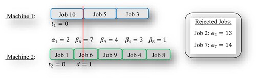
The resulting optimal solution (see Figure 1) consists of 2 rejected jobs (jobs 2 and 7), and 8 scheduled jobs (3 jobs on machine 1, and 5 jobs on machine 2). The optimal case is Case 1, i.e. the starting times of the job sequences on machines 1 and 2 are: $t_1=t_2=0$. The optimal due-date value is $d=1$. The job sequence on machine 1 is (10,5,3), and on machine 2 is (1,6,9,4,8). The rejection cost is 27, the earliness-tardiness and due-date cost of the processed jobs is 45.52, and the total optimal cost is 72.52.

Figure 1. Optimal solution for Example 1.

4. The case of a fixed (given) due-date

In this section the problem is modified to a setting in which the due-date is given (and not a decision variable). Consequently, the due-date cost is removed. We thus focus on the problem: $\begin{array}{rl}{Q}_2|d_j& =d\mathrm{given},p_{1j}=1,p_{2j}=s,\mathrm{rejection}|\sum _{j\in P}\left({\alpha }_j{E}_j+{\text{β}}_j{T}_j\right)+\sum _{j\in R}{e}_j\end{array}$We note that the classical single-machine CON problem for a given due-date (with job-dependent processing times) is NP-hard if the due-date is restrictive (i.e. sufficiently small); see Hall, Kubiak, and Sethi (1991). We show in the following that in our setting, the problem remains polynomially solvable even with a given restrictive due-date.

As above, the solution procedure consists of a sequential solution of linear assignment problems. We introduce the solution for a fixed number of processed job ($|P|$). For a given $|P|$ ($0\le |P|\le n$), we create an assignment matrix with the following five blocks: ($i$) the block of early jobs on machine 1: $n\times |P|$; ($\mathrm{ii}$) the block of tardy jobs on machine 1: $n\times |P|$; ($\mathrm{iii}$) the block of early jobs on machine 2: $n\times |P|$; ($\mathrm{iv}$) the block of tardy jobs on machine 2: $n\times |P|$; ($v$) the block of the rejected jobs: $n\times n$. (Note that, in fact, the number of early jobs on machine 1 is bounded by $d$ and the number of early jobs on machine 2 is bounded by $\frac{d}{s}$, which may reduce the number of columns in the matrix.) The costs in each block ($\mathrm{Cost}\left(i,j\right)$) are calculated as above.

The assignment problem for a given $|P|$ value is denoted $\mathrm{LAP}\left(|P|\right)$. $\mathrm{LAP}\left(|P|\right)$ is solved for each $|P|$ value, and the total loads of the early jobs on both machines are examined. Let $n_1^E$ and $n_2^E$ denote the number of early jobs on machines 1 and 2, respectively. Then, the total early loads on the machines are $n_1^E$ ans $n_2^{E}s$, respectively. If both loads in a specific solution are smaller than the due-date ($n_1^E\le d$ and $n_2^{E}s\le d$), then the due-date is defined as non-restrictive, the solution is feasible, and is registered as a candidate for being optimal.

The solution procedure starts with solving the linear assignment problem for $|P|=0$. This clearly leads to a feasible solution since no jobs are processed. Then we increase $|P|$ by 1 and solve again. As long as the early loads on both machines are smaller than the due-date, the due-date is non-restrictive and the resulting schedule is feasible. If for some value, say $|P|=x$, at least one of the early loads exceeds $d$, then the due-date is defined as restrictive. In these settings there are three cases that need to be considered:

Case 1: ${\mathit{t}}_1={\mathit{t}}_2=0$.

In this setting the due-date does not necessarily coincide with a job completion time on both machines. This is the case e.g. when the due-date is sufficiently small, such that increasing either $t_1$ or $t_2$ increases the total cost.

Case 2: ${\mathit{t}}_1=0,{\mathit{t}}_2>0$.

In this case the due-date coincides with a job completion time on machine 2. The proof is by a standard perturbation: if the due-date does not coincide with a job completion time on machine 2 then either increasing or decreasing $t_2$ until it does cannot increase the cost. Further reduction of $t_2$ may lead to $t_2=0$, which is Case 1.

Case 3: ${\mathit{t}}_1>0,{\mathit{t}}_2=0$.

In this case the due-date coincides with a job completion time on machine 1. As above, the proof is based on perturbation arguments.

Running Time:

For a given value $|P|$ of processed jobs, and a given number of jobs assigned to machine 1 ($n_1$), a linear assignment problem, denoted $\mathrm{LAP}\left(|P|,n_1\right)$ needs to be solved. Since $0\le n_1\le |P|\le n$, a total of $O\left(n^2\right)$ assignment problems are solved. Hence, the total running time of the solution algorithm is $O\left(n^5\right)$.

In fact, the actual running time is smaller due to the following bounds on the number of jobs assigned to machine 1:

Theorem 4.1:

The number of jobs assign to machine 1 is: $\frac{\left(|P|-1\right)s-1}{1+s}\le n_1\le \frac{\left(|P|+1\right)s+1}{1+s}$.

Proof.

The load on machine 1 cannot exceed the load on machine 2 by more than $s+1$. If this property does not hold, then $C_{\max }^1>C_{\max }^2+s$, or $t_1<t_2-1$, or both. If $C_{\max }^1>C_{\max }^2+s$, it is worthwhile moving the last job on machine 1 to be the last job on machine 2. If $t_1<t_2-1$, it is worthwhile moving the first job on machine 1 to be the first job on machine 2. We obtain that $n_1\le n_{2}s+s+1$. Thus, $n_1\le \frac{\left(|P|+1\right)s+1}{1+s}$. Since $n_1$ is an integer, we conclude that $n_1\le \frac{\left(|P|+1\right)s+1}{1+s}$.

Similarly, the load on machine 2 cannot exceed the load on machine 1 by more than $s+1$. [If $C_{\max }^2>C_{\max }^1+1$, it is worthwhile moving the last job on machine 2 to be the last job on machine 1. If $t_2<t_1-s$, it is worthwhile moving the first job on machine 2 to be the first job on machine 1.] Therefore, $n_{2}s\le n_1+s+1$. It follows that $n_1\ge \frac{\left(|P|-1\right)s-1}{1+s}$. Since $n_1$ is an integer, we conclude that $n_1\ge \frac{\left(|P|-1\right)s-1}{1+s}$.

Numerical Example 2:

As above, we considered a 10 job example. The machine speeds are identical to those considered in Example 1 (1 and $0.72$, on machines 1 and 2, respectively). The earliness, tardiness and rejection costs are also identical to those of Example 1.

We assumed first that the (given) due-date value is $d=\mathrm{3.5.}$ In the optimal solution, all jobs are processed (i.e. no rejected jobs). 4 jobs are assigned to machine 1 (2 are early), and 6 jobs are assigned to machine 2 (4 are early). The starting times of the job sequences on machines 1 and 2 are: $t_1=1.5$, and $t_2=0.62$, i.e. the due-date in this case is non-restrictive. The job sequence on machine 1 is (7,6,9,8), and on machine 2 is (4,1,2,10,5,3). The optimal total (earliness-tardiness) cost is 23.4.

Then, a smaller due-date value was assumed: $d=0.9$. This is clearly a restrictive due-date, since it is strictly smaller than the early loads obtained in the above solution.

In the optimal solution, 9 jobs are processed and a single job is rejected. 4 jobs are assigned to machine 1 (all jobs are tardy), and 5 jobs are assigned to machine 2 (1 job is early). The optimal case is Case 1: $t_1=t_2=0$. The job sequence on machine 1 is (10,5,4,8), and on machine 2 is (1,6,2,9,3). Job 7 is rejected. The total earliness-tardiness cost is 39.46, the total rejection is 14, and the optimal total cost is 53.46.

5. An extension to $m$ machines ($m\ge 3$)

The solution procedure introduced in this paper is for the case of $m=2$ uniform machines. We show in the following how to extend this solution to the more general setting of $m\ge 3$ machines. For convenience we focus on the case of $m=3$, and the machines speed are denoted by $s_1,s_2$ and $s_3$. Thus, the problem studied here is: $\begin{array}{rl}{Q}_3|d_j& =d,p_{1j}=s_1,p_{2j}=s_2,p_{3j}=s_3,\mathrm{rejection}|\sum _{j\in P}\left({\alpha }_j{E}_j+{\text{β}}_j{T}_j+\mathrm{\gamma d}\right)+\sum _{j\in R}{e}_j\end{array}$

Without loss of generality, the machines speeds are assumed to be: $s_1=1\ge s_2\ge s_3$.

Denote the starting times on the three machines by $t_1,t_2$ and $t_3$, respectively. The number of cases which are candidates for being optimal is calculated in the following:

($\mathrm{i}$) When $t_1=t_2=t_3=0$, the due-date may coincide with a job completion time on each of the machines. Thus, there are three relevant cases.

($\mathrm{ii}$) When $t_1=t_2=0$, and $t_3>0$, the due-date may coincide with either a job completion time on machine 1 and a job completion time on machine 3, or it may coincide with a job completion time on machine 2 and a job completion time on machine 3. Thus, there are two cases. This setting is equivalent to the case that $t_1=t_3=0$, and $t_2>0$, and to the case that $t_2=t_3=0$, and $t_1>0$. This leads to additional six cases.

($\mathrm{iii}$) When $t_1=0$, and $t_2,t_3>0$, the due-date coincides with a job completion time on all three machines. Similar setting are that of $t_2=0$, and $t_1,t_3>0$, and also that of $t_3=0$, and $t_1,t_2>0$. This leads to three cases.

It follows that the total number of cases that need to be considered for a three machine setting is 12. A similar counting procedure can be done for settings containing more machines. While the actual computational effort increases significantly for larger $m$ values due to the large number of assignment problems that need to be solved, for a fixed $m$ value the running time remains polynomial in $n$.

6. Special cases

6.1. The special case of a single machine

The single machine setting is: $\begin{array}{rl}1/d_j& =d,p_j=1,\mathrm{rejection}/\sum _{j\in P}\left({\alpha }_j{E}_j+{\text{β}}_j{T}_j+\mathrm{\gamma d}\right)+\sum _{j\in R}{e}_j\end{array}$

In this setting, an optimal schedule always starts at time zero, all jobs have identical processing times (of e.g. 1), and the due-date coincides with a job completion time. Hence, only a single case is relevant (rather than the four cases, which need to be considered for the case of two machines). However, linear assignments problems need to be solved for all $|P|$ and $d$ values (both bounded by $n$), implying that $O\left(n^2\right)$ linear assignment problems are solved, and the running time remains $O\left(n^5\right)$.

6.2. The special case of a parallel identical machines

The setting of parallel identical machines is: $\begin{array}{rl}P2/d_j& =d,p_j=1,\mathrm{rejection}/\sum _{j\in P}\left({\alpha }_j{E}_j+{\text{β}}_j{T}_j+\mathrm{\gamma d}\right)+\sum _{j\in R}{e}_j\end{array}$

In the case of parallel identical machines, the processing time of each job is 1 on all the machines. For simplicity, we focus on the case of two parallel identical machines. For a given number of processed jobs $|P|$, it is easily verified that an optimal schedule exists with equal allocation of jobs to machines. In the case that $|P|$ is even, $|P|/2$ jobs are assigned to each machine, and in the case that $|P|$ is odd, $\lfloor |P|/\phantom{|P|2}2\rfloor$ jobs are assigned to machine 1 and $\lfloor |P|/\phantom{|P|2}2\rfloor +1$ jobs are assigned to machine 2. There is a major difference between this case and the more general case of uniform machines: in an optimal schedule for the case of two parallel machines, the due-date coincides with the completion time of a job on both machines. (Note also that in the case of an even number of processed jobs, the starting time of the first job on both machines is zero. In the case of an odd number of processed jobs, the starting time of the first job on machine 1 is zero, and the starting time of the first job on machine 2 is either zero or one.) For a given number of processed jobs and for a given due-date value, an assignment problem needs to be solved. Hence, despite the fact that there is no need to examine four cases (as in the case of uniform machines), the total complexity of this problem remains $O\left(n^5\right)$.

6.3. The special case of symmetric costs

We focus now on the special case that the earliness and the tardiness unit costs of a given job are identical: ${\alpha }_j={\text{β}}_j=w_j,j=1,\dots ,n$. The problem becomes: $\begin{array}{rl}{Q}_2/d_j& =d,p_{1j}=1,p_{2j}=s,\mathrm{rejection}/\\ & \times \sum _{j\in P}\left(w_j|d-C_j|+\mathrm{\gamma d}\right)+\sum _{j\in R}{e}_j\end{array}$

In this setting, all $|P|$ values need to be considered, all four cases are relevant, and for a given allocation of jobs to machines, all $d$ values need to be covered ($d\le n_1$ in Cases 1 and 3, and $d\le n_{2}s$ in Cases 2 and 4). For a given $d$ value, the assignment of the jobs to positions does not require a solution of a linear assignment problem. In fact, the assignment is done in the following greedy manner. Assuming that jobs were initially sorted in a non-increasing order of weights, the first job (with the largest weight) is assigned to have the closest completion time to $d$ (on any of the machines), the second job (with the second-to-largest weight) is assigned to have the second-to-closest completion time to $d$, etc. This procedure of solving the problem for a given $|P|$ and the relevant case, is performed in $O\left(n\right)$ time. Since all $|P|$ and all $d$ values need to be considered ($|P|\le n$ and $d\le n_1$ or $d\le n_{2}s$), the greedy assignment is performed $O\left(n^2\right)$ times, leading to total running time of $O\left(n^3\right)$. (The initial sorting procedure of the job weights is performed in $O\left(\mathrm{nlogn}\right)$ time, and does not change this running time.)

6.4. The special case of job-independent earliness-tardiness costs

In this special case, we assume that ${\alpha }_j=\alpha$ and ${\text{β}}_j=\text{β},j=1,\dots ,n$. The problem is reduced to: $\begin{array}{rl}{Q}_2|d_j& =d,p_{1j}=1,p_{2j}=s,\mathrm{rejection}|\\ & \sum _{j\in P}\left(\alpha E_j+\text{β}{T}_j+\mathrm{\gamma d}\right)+\sum _{j\in R}{e}_j\end{array}$

Note that for a given $|P|$ value, this problem was solved by Mosheiov and Sarig (2009) in constant time. Since all $|P|\left(\le n\right)$ values need to be considered, the total computational effort required for solving this problem is $O\left(n\right)$.

7. Conclusion

We studied a common due-date assignment problem on two parallel uniform machines. We assumed identical processing times and job-dependent and asymmetric earliness and tardiness unit costs. The option of job-rejection is available. The goal is to minimise total earliness-tardiness cost of the scheduled jobs, the cost of the common due-date, and total rejection cost. We introduced an $O\left(n^5\right)$ solution procedure (based on solving $O\left(n^2\right)$ linear assignment problems), and is therefore polynomial in the number of jobs.

A possible topic for future research is the extension of this model to more complicated machine settings, such as an $m$-machine flowshop with machine-dependent speeds or a flexible flowshop. The model studied here with an additional assumption on an upper bound on the total permitted rejection cost (which is easily shown to be NP-hard), is another challenging topic.

Disclosure statement

No potential conflict of interest was reported by the author(s).

Data availability statement

Not relevant for this paper.

Additional information

Funding

The first author was supported by the Israel Science Foundation (Grant No.2505/19) and by the Deutsche Forschungsgemeinschaft (DFG, German Research Foundation) – Project Number 452470135.

Notes on contributors

Gur Mosheiov

Gur Mosheiov is a full professor in The School of Business Administration of The Hebrew University, Jerusalem, Israel. He holds a BSc in Mathematics and Physics and an MBA from The Hebrew University. He completed his PhD in The Graduate School of Business, Columbia University, NYC. Served as the head of the MBA program and the vice dean in The School of Business Administration of The Hebrew University. His research area is combinatorial optimisation, with a focus on production scheduling.

Assaf Sarig

Assaf Sarig is a senior lecturer at the College of Law & Business, and a researcher in the field of combinatorial optimisation, mainly in production scheduling. He holds a BA in Statistics and Economics (2003), and MA in Statistics and Business Administration (2005), from The Hebrew University, Jerusalem, Israel. He completed his PhD in Operations Research in The School of Business Administration of The Hebrew University. His research focuses on various types of scheduling problems and maintenance activity.

References

- Arık, O. A., and M. D. Toksarı. 2018. “Multi-Objective Fuzzy Parallel Machine Scheduling Problems Under Fuzzy Job Deterioration and Learning Effects.” International Journal of Production Research 56 (7): 2488–2505. doi:10.1080/00207543.2017.1388932
- Bülbül, K., S. Kedad-Sidhoum, and H. Şen. 2019. “Single-Machine Common Due Date Total Earliness/Tardiness Scheduling with Machine Unavailability.” Journal of Scheduling 22 (5): 543–565. doi:10.1007/s10951-018-0585-x
- Chen, X., Y. Liang, M. Sterna, W. Wang, and J. Błażewicz. 2020. “Fully Polynomial Time Approximation Scheme to Maximize Early Work on Parallel Machines with Common Due Date.” European Journal of Operational Research 284 (1): 67–74. doi:10.1016/j.ejor.2019.12.003
- Falq, A. E., P. Fouilhoux, and S. Kedad-Sidhoum. 2021. “Mixed Integer Formulations Using Natural Variables for Single Machine Scheduling Around a Common Due Date.” Discrete Applied Mathematics 290: 36–59. doi:10.1016/j.dam.2020.08.033
- Gao, F., M. Liu, J. J. Wang, and Y. Y. Lu. 2018. “No-Wait Two-Machine Permutation Flow Shop Scheduling Problem with Learning Effect, Common Due Date and Controllable Job Processing Times.” International Journal of Production Research 56 (6): 2361–2369. doi:10.1080/00207543.2017.1371353
- Gerstl, E., and G. Mosheiov. 2017. “Single Machine Scheduling Problems with Generalized Due-Dates and Job-Rejection.” International Journal of Production Research 55 (11): 3164–3172. doi:10.1080/00207543.2016.1266055
- Gerstl, E., and G. Mosheiov. 2021. “The Single Machine CON Problem with Unavailability Period.” International Journal of Production Research 59 (3): 824–838. doi:10.1080/00207543.2019.1709672
- Gordon, V., J. M. Proth, and C. Chu. 2002. “A Survey of the State-of-the-Art of Common Due Date Assignment and Scheduling Research.” European Journal of Operational Research 139 (1): 1–25. doi:10.1016/S0377-2217(01)00181-3
- Hall, N. G., W. Kubiak, and S. P. Sethi. 1991. “Earliness–Tardiness Scheduling Problems, II: Deviation of Completion Times About a Restrictive Common Due Date.” Operations Research 39 (5): 847–856. doi:10.1287/opre.39.5.847
- Kellerer, H., K. Rustogi, and V. A. Strusevich. 2020. “A Fast FPTAS for Single Machine Scheduling Problem of Minimizing Total Weighted Earliness and Tardiness About a Large Common due Date.” Omega 90: 101992. doi:10.1016/j.omega.2018.11.001
- Kuhn, H. W. 1955. “The Hungarian Method for the Assignment Problem.” Naval Research Logistics Quarterly 2 (1-2): 83–97. doi:10.1002/nav.3800020109
- Li, S. S., and R. X. Chen. 2020. “Scheduling with Common Due Date Assignment to Minimize Generalized Weighted Earliness–Tardiness Penalties.” Optimization Letters 14: 1681–1699. doi:10.1007/s11590-019-01462-5
- Li, Z., R. Y. Zhong, A. V. Barenji, J. J. Liu, C. X. Yu, and G. Q. Huang. 2019. “Bi-Objective Hybrid Flow Shop Scheduling with Common due Date.” Operational Research 21: 1153–1178.
- Liu, M., S. Wang, F. Zheng, and C. Chu. 2017. “Algorithms for the Joint Multitasking Scheduling and Common Due Date Assignment Problem.” International Journal of Production Research 55 (20): 6052–6066. doi:10.1080/00207543.2017.1321804
- Lv, D. Y., and J. B. Wang. 2021. “Study on Proportionate Flowshop Scheduling with Due-Date Assignment and Position-Dependent Weights.” Optimization Letters 15 (6): 2311–2319.
- Mor, B. 2018. “Minmax Common Due-Window Assignment and Scheduling on a Single Machine with Two Competing Agents.” Journal of the Operational Research Society 69 (4): 589–602.
- Mor, B. 2019. “Minmax Scheduling Problems with Common due-Date and Completion Time Penalty.” Journal of Combinatorial Optimization 38 (1): 50–71. doi:10.1007/s10878-018-0365-8
- Mosheiov, G., and S. Pruwer. 2021. “On the Minmax Common-Due-Date Problem: Extensions to Position-Dependent Processing Times, job Rejection, Learning Effect, Uniform Machines and Flowshops.” Engineering Optimization 53 (3): 408–424. doi:10.1080/0305215X.2020.1735380
- Mosheiov, G., and A. Sarig. 2009. “Due-Date Assignment on Uniform Machines.” European Journal of Operational Research 193 (1): 49–58. doi:10.1016/j.ejor.2007.10.043
- Mosheiov, G., and U. Yovel. 2006. “Minimizing Weighted Earliness–Tardiness and Due-Date Cost with Unit Processing-Time Jobs.” European Journal of Operational Research 172 (2): 528–544. doi:10.1016/j.ejor.2004.10.021
- Nasrollahi, V., G. Moslehi, and M. Reisi-Nafchi. 2022. “Minimizing the Weighted Sum of Maximum Earliness and Maximum Tardiness in a Single-Agent and Two-Agent Form of a Two-Machine Flow Shop Scheduling Problem.” Operational Research, 1–40.
- Rocholl, J., and L. Mönch. 2021. “Decomposition Heuristics for Parallel-Machine Multiple Orders Per Job Scheduling Problems with a Common Due Date.” Journal of the Operational Research Society 72 (8): 1737–1753.
- Shabtay, D., N. Gaspar, and M. Kaspi. 2013. “A Survey on Offline Scheduling with Rejection.” Journal of Scheduling 16 (1): 3–28. doi:10.1007/s10951-012-0303-z
- T’kindt, V., L. Shang, and F. Della Croce. 2020. “Exponential Time Algorithms for Just-in-Time Scheduling Problems with Common Due Date and Symmetric Weights.” Journal of Combinatorial Optimization 39 (3): 764–775. doi:10.1007/s10878-019-00512-z
- Xiong, X., D. Wang, T. C. Edwin Cheng, C. C. Wu, and Y. Yin. 2018. “Single-Machine Scheduling and Common Due Date Assignment with Potential Machine Disruption.” International Journal of Production Research 56 (3): 1345–1360. doi:10.1080/00207543.2017.1346317