Inventory management for stockout-based substitutable products under centralised and competitive settings

Abstract

Inventory planning in fashion markets is highly challenging, owing to uncertain demand; yet, in making inventory decisions, retailers may be able to capitalise on high substitutability between products. This research develops single-period inventory-management models describing a market with two substitutable products, under stockout-based substitution; i.e. when a customer’s preferred product is out-of-stock, s/he may choose to purchase the substitute. Two settings are considered: centralised (a single retailer who sells both products) and competitive (two retailers, each selling one product). For each setting, we derive closed-form analytical solutions for the inventory levels that maximise expected profit. The model is further enriched with sales data from an online apparel retailer offering substitutable products (a sneaker in different colours), and we analyse the sensitivity of the optimal inventory levels and profits to parameter values. Key findings include the following: (i) Under competitive conditions, both retailers always order positive inventory so as not to lose customers. However, in a single-retailer setting, there are situations in which the retailer orders inventory for only one product. (ii) The optimal inventory levels and corresponding profits are highly sensitive to consumers’ willingness to substitute between products. These findings provide concrete insights that can guide fashion brands’ inventory-management decisions.

KEYWORDS:

• Inventory management
• stockout-based substitution
• fashion industry
• game theory
• supply chain management

1. Introduction

The fashion market is characterised by dynamic and volatile demand conditions, in which new products are released every sales period, rendering older merchandise obsolete – yet, at the same time, the desirability of new collections, and thus the demand for the corresponding products, is uncertain. These conditions make it challenging for retailers to successfully plan their inventories, i.e. to determine the quantity and assortment (e.g. colours and patterns) of items to offer in each sales period (Ho et al. 2015; Wang et al. 2022). In making such decisions, retailers must further consider another key feature of fashion markets: the high potential for substitutability between products. For example, fashion products are often manufactured in a variety of colours, meaning that if a specific garment that a consumer wishes to buy is out of stock, they might switch and buy the same garment in a different colour (Ergin, Gümüş, and Yang 2022).

A consumer’s sensitivity to substitutability may determine the extent to which he or she is likely to engage in such substitution (Caro and Gallien 2010; Zhang et al. 2020). Willingness to accept substitutes may be particularly high in fast fashion markets, where collections change rapidly over a finite season (Schlapp and Fleischmann 2018). In these markets, when consumers are looking for a specific product but find that it is out of stock, they may be faced with a choice between purchasing the product in a different colour or not purchasing it at all – as the product is unlikely to return (Choi and Guo 2018).

Herein, taking these considerations into account, we study optimal inventory decisions of fashion retailers aiming to maximise their expected profits. Our work comprises two main components: an analytical modelling component and an empirical study. For the analytical component, we model a market in which two substitutable fashion products are sold. We examine two scenarios, each of which we describe with a single-period inventory model: The first scenario is a centralised setting in which a single retailer offers both substitutable products. Each customer has a preferred product, and, if that product is out of stock, the customer may either purchase the substitute (from the same retailer) or, alternatively, buy nothing. The second scenario is a competitive setting with two competing retailers, each of whom sells one of the two substitutable products. When a customer’s preferred product is out of stock, the customer may choose to buy the substitutable product from the competing retailer or not buy any product at all. In each model, on the basis of a set of given parameter values (e.g. the customer’s willingness to substitute one product for the other, the price and unit cost of each product, etc.), the retailer(s) choose the inventory level(s) that maximise profits. Our work extends the inventory model of Koren, Perlman, and Shnaiderman (2022), which considered only the second of the two scenarios we describe, namely, a competitive setting with two substitutable products, each offered exclusively by a different retailer. We investigate how this scenario compares to the centralised setting in terms of the optimal inventory level for each product, as well as the corresponding profits. This comparison can provide insights into how inventory management strategies might differ between a retailer that is an exclusive carrier of a particular product (e.g. a designer shop or even a chain retailer, such as The Gap, selling its own branded items) versus a retailer that carries products that are available through multiple competing retailers (e.g. products manufactured by national or global brands such as Nike or Adidas).

Next, in the empirical component of this research, we derive the actual demand distributions of two substitutable fashion products offered by a fast-fashion retailer (in our model, the joint demand distribution is represented by a general function). Then, given these demand distributions, as well as other real-world data regarding product prices, we examine how the optimal inventory levels and corresponding expected profits are affected by three parameters: substitution rate (customers’ willingness to purchase a substitute when their preferred product is out of stock), unit selling price, and the correlation between the demand levels of the two products.

The main contributions of this paper are as follows: (i) Closed-form analytical solutions are obtained for optimal inventory levels in centralised and competitive settings; in both cases, we prove that the objective functions are concave, so that a unique optimal solution exists. (ii) We estimate the joint probability of the demand distribution based on data from an online apparel retailer regarding the sales of two substitutable products. (iii) We characterise the impact of stockout-based substitution rate on optimal inventory levels and profits under centralised and competitive cases. A nonintuitive result is the finding that when customers’ flexibility regarding substitution of a particular product is low, the optimal inventory order size of that product is larger in the case of a single retailer than in the competitive setting. The models we develop, as well as the findings of our analysis, can be of value to fashion retailers seeking to plan their inventories in an uncertain market.

2. Literature review

2.1. Background: inventory management in the fashion industry

In general, the main objective of inventory management is to ensure that demand is met in a manner that minimises profit loss – so as to avoid being left with a surplus of unsold goods at the end of the season on the one hand, while preventing a shortage of popular items due to excessive demand (Shen et al. 2016). In the fashion industry, effective inventory management entails a complex process of identifying customers’ future tastes and preferences, e.g. by tracking factors that might influence these preferences (Ambilkar et al. 2022; Ko, Costello, and Taylor 2019; Singh and Verma 2018). On the basis of this information about consumer preferences, coupled with information regarding the current state of the market, as well as historical data (which is commonly used in trend forecasting; see Loureiro, Miguéis, and da Silva 2018), designers and manufacturers decide which items and how many to produce, and retailers decide what to stock (DuBreuil and Lu 2020; Shokouhyar et al. 2021; Yamazaki, Shida, and Kanazawa 2016). Yet, ultimately, decisions about the production and stocking of multitudes of new designs are based on incomplete information that cannot provide a definitive indication of products’ future success (Ren, Chan, and Siqin 2020; Wen, Choi, and Chung 2019).

Using historical data for the purpose of trend forecasting is a common tool (Loureiro, Miguéis, and da Silva 2018). In the empirical portion of our study, we similarly incorporate sales history to obtain an understanding of how the demand for two substitutable products is expected to behave.

2.2. Inventory management models with product substitution

Starting from a seminal paper written by Parlar (1988), extensive research has been devoted to modelling various inventory management problems in the presence of product substitution. A review by Shin et al. (2015) identifies four criteria according to which models in this research stream can be classified. The first criterion is the modelling objective and, more broadly, the type of problem being addressed – e.g. assortment planning, inventory decisions, capacity planning, or pricing decisions. A second criterion identified by Shin et al. (2015) is the identity of the party who initiates the substitution (the ‘decision-maker’). Specifically, substitution can be initiated either by the firm (as in the case of a company that manufactures a high-end product and decides to offer a similar, lower-end product to a different customer segment) or by the customer (e.g. when a customer faced with multiple substitutable alternatives selects one based on preference). The third criterion relates to the direction of substitutability: one-way (in which product A can be substituted for product B but not vice versa), or two-way (in which products can be substituted in either direction). The fourth criterion is the mechanism of substitution, which, according to Shin et al. (2015), can fall into three main categories: (i) price-based substitution, in which a customer generally prefers a particular product but may select an alternative product because it is cheaper; (ii) assortment-based substitution, in which a store does not carry the customer’s preferred product, and the customer may decide to substitute a product that the store does carry (Martínez-de-Albéniz and Kunnumkal 2022); and (iii) inventory stockout-based substitution, in which, when the customer’s preferred product is out of stock, he or she can buy a substitutable product. Transchel (2017) further refers to assortment-based substitution as ‘static’ substitution, as, in this scenario, the consumer’s preferred item is not included in the retailer’s predetermined, static assortment, and the consumer must decide whether to substitute it with an alternative; see Hübner (2017) and Kök, Fisher, and Vaidyanathan (2015). In turn, Transchel (2017) refer to inventory-based substitution as ‘dynamic’, because in this scenario, the consumer’s preferred item is typically included in the retailer’s assortment, but is currently not available (e.g. Chen and Chao 2020; Goyal, Levi, and Segev 2016; Honhon, Gaur, and Seshadri 2010). Stockout-based (dynamic) substitution has been explored in diverse types of inventory-related problems, including pricing decisions in the presence of store capacity constraints (Gümüş, Kaminsky, and Mathur 2016), inventory routing and transshipment decisions (Achamrah, Riane, and Limbourg 2022; Li and Li 2018), inventory distribution processes (Caro and Gallien 2010; Wang and Zhang 2021), inventory management (Transchel et al., 2017; Perlman 2019), and production scheduling (Zeppetella et al. 2017).

Notably, some studies modelling inventory management may fall into multiple categories for a particular criterion in Shin et al.’s (2015) taxonomy. In particular, some simultaneously consider multiple types of inventory-related decisions – e.g. inventory quantity and pricing – and, in some cases, multiple forms of substitution. Examples include the works of Besbes and Sauré (2016) Zhao and Zhao (2016), who modelled a scenario in which retailers compete in both assortment and prices and must choose which product assortment to offer, given display constraints. Dong et al. (2020) developed an inventory-pricing model in which a retailer who offers two substitutable products seeks to select the prices and inventory levels for those products so as to maximise expected profits. Recently, Hammami et al. (2022) studied inventory decisions for a retailer offering substitutable products that differ in delivery time and price, under hybrid distribution (i.e. rapid delivery from the retailer’s stock versus slower delivery via drop shipping).

According to the taxonomy described above, the models developed in the current research can be categorised as inventory planning (i.e. order quantity) decision models under dynamic, inventory stockout-based substitution, in which the customer initiates the substitution decision, and substitutability is bidirectional. Specifically, this research develops single-period inventory-management models. Similarly to Parlar (1988), we seek to identify optimal order quantities in a market with two substitutable products. However, Parlar (1988) assumed that the demand for each product is independent of the demand for the other product, while we consider a general joint probability density function of the demand. Our model is further enriched with sales data from an online apparel retailer offering substitutable products (a sneaker in different colours). In a numerical analysis based on these data, we are able to fit a specific joint demand function, estimate the correlation between the demand level of the two products, and perform sensitivity analysis of the optimal inventory levels and profits to this parameter.

As noted in the introduction, our study addresses both a centralised scenario of product substitution – in which consumers accept product substitutes offered by the same retailer – and a scenario in which a decision to accept a substitute for an out-of-stock product entails a decision to patronise a different store. Prior studies have examined either the former or the latter. For example, Li et al. (2023) examined how demand spills over to substitute products (specifically, products of different sizes) offered by the same retailer. Ergin, Gümüş, and Yang (2022), in turn, examined the dynamics of substitution across stores, and found that the likelihood of such substitution is strongest when customers first observe the lack of stock, and decreases over time. Ovezmyradov and Kurata (2019) modelled customers’ responses to the stockout of fashion products and showed how a retailer can maximise profit by offering substitutable products at multiple stores. Other models considered two phases of selection; the consumer first chooses where to shop (i.e. brick and mortar store or online store), and subsequently selects the product (e.g. Gupta, Ting, and Tiwari 2019; Wan et al. 2018). To our knowledge, our work is among the few to compare how, in the presence of stockout-based substitution, optimal inventory decisions in a multi-retailer setting differ from those in a centralised setting.

3. Models

In what follows, we develop and analyse two separate inventory models representing different scenarios in a market in which two substitutable products are sold (product 1 and product 2), and substitution is of a dynamic inventory stockout-based nature. That is, a customer may choose to substitute one product for the other only in the event that her preferred product is out of stock. In each model, a retailer (or retailers) must set the inventory level(s) of the product(s) they offer so as to maximise expected profit. The first model (subsection 3.1) focuses on a centralised setting, in which a single retailer sells both substitutable products. Such centralisation can occur in cases in which a retailer sells its own branded products that are not available through competing retailers, or, as suggested by Parlar (1988), in cases in which one retailer takes over another, or establishes a collaboration with another retailer. In the latter arrangement, neither retailer incurs any penalties if the ‘competitor’ fulfils the demand of the other retailer. The second model (subsection 3.2), based on the work of Koren, Perlman, and Shnaiderman (2022), examines a competitive setting with two retailers, each offering only one of the two products. In subsection 3.3, the two models are compared, and we examine the impact of customers’ substitution rate on the retailers’ optimal inventory levels.

The notations and the decision variables used in the models are as follows:

• i – indicator for a specific product, i ε {1,2}; in the two-retailer model, the term ‘retailer i’ denotes the retailer that offers product i.

• Q_i – Inventory level of product i (a decision variable)

• X_i – Demand for product i (a random variable with realisation x_i)

• f – The joint probability density function of X₁ and X₂

• p_i – Unit selling price of product i

• c_i – Order cost of product i

• s_i – Salvage value of product i

• δ_i – The stockout-based substitution rate, defined as customers’ probability (i.e. their willingness) to buy product 3-i if product i is out of stock, and given that product 3 – i is available in the market.

• π – Retailer’s profit; in the two-retailer model, π_i denotes the profit of retailer i.

Products are assumed to have a shelf life of one selling period and zero units of inventory prior to the start of the selling period. In addition, p_i > c_i > s_i ≥ 0, i = 1, 2. We also assume that if the inventory level of product i, Q_i, is less than the demand X_i (i.e. is out of stock), each customer must decide whether to purchase the product substitute instead, i.e. product 3 – i (if available). The customer purchases the substitute with probability δ_i, or buys nothing, with probability 1– δ_i.

3.1. Inventory model for a single retailer

Consider a single retailer who sells both types of substitutable products, i.e. product 1 and product 2.

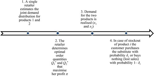
The retailer, who orders all inventory prior to the selling period, seeks to choose optimal order quantities $Q_1^{\ast }$ and $Q_2^{\ast }$ that maximise her profit π, given the values of the other variables. See sequence of events in Figure 1.

Figure 1. Sequence of events for centralised setting.

Overview of the centralised setting's events in a timeline. In the first event, a joint demand distribution is estimated and in the last event, the customer makes a purchase or not.

3.1.1. Profit outcomes for different values of inventory and demand

We first identify four general scenarios regarding the retailer’s profit (a random variable) for specific values of the inventory levels Q₁ and Q₂, defined in relation to the random demand levels X₁ and X₂.

1. If X₁≤ Q₁ and X₂≤ Q₂, each customer receives his or her preferred product, and the retailer's profit is (1) $\begin{array}{rl}& \pi (Q_1,Q_2,X_1,X_2)=(p_1-s_1)X_1+(p_2-s_2)X_2\\ & -(c_1-s_1)Q_1-(c_2-s_2)Q_2\end{array}$(1)

2. If X₂> Q₂ and X₁≤ Q₁–δ₂(X₂ – Q₂), the inventory of product 2 does not meet the demand for that product. On the other hand, the inventory level of product 1 satisfies both the original demand for that product and the demand among customers who prefer product 2 but find that it is unavailable, and are willing to buy product 1 instead. Thus, the retailer’s profit is: (2) $\begin{array}{rl}& \pi (Q_1,Q_2,X_1,X_2)=(p_1-s_1)[X_1+{\delta }_2(X_2-Q_2)]\\ & -(c_1-s_1)Q_1+(p_2-c_2)Q_2\end{array}$(2)

3. Similarly, if X₁> Q₁ and X₂≤ Q₂–δ₁(X₁ – Q₁), (3) $\begin{array}{rl}& \pi (Q_1,Q_2,X_1,X_2)=(p_2-s_2)[X_2+{\delta }_1(X_1-Q_1)]\\ & -(c_2-s_2)Q_2+(p_1-c_1)Q_1\end{array}$(3)

4. Otherwise, all the inventory is sold, and the profit is equal to (4) $\begin{array}{r}\pi (Q_1,Q_2,X_1,X_2)=p_1{Q}_1+p_2{Q}_2-c_1{Q}_1-c_2{Q}_2\end{array}$(4)

3.1.2. Expected profit maximisation

Based on (1)–(4), the retailer's expected profit is (5) $\begin{array}{rl}& Z(Q_1,Q_2)\\ & =\text{E}[\pi (Q_1,Q_2,X_1,X_2)]\\ & ={\int }_0^{\mathrm{\infty }}{\int }_0^{\mathrm{\infty }}\pi (Q_1,Q_2,x_1,x_2)f(x_1,x_2)d{x}_{2}d{x}_1\\ & ={\int }_0^{Q_1}[{\int }_0^{Q_2}((p_1-s_1)x_1+(p_2-s_2)\\ & \times x_2+s_1{Q}_1+s_2{Q}_2)f(x_1,x_2)d{x}_2\\ & +{\int }_{Q_2}^{Q_2+\frac{Q_1-x_1}{{\delta }_2}}((p_1-s_1)(x_1+{\delta }_2(x_2-Q_2))\\ & +p_2{Q}_2+s_1{Q}_1)f(x_1,x_2)d{x}_2\\ & +{\int }_{Q_2+\frac{Q_1-x_1}{{\delta }_2}}^{\mathrm{\infty }}(p_1{Q}_1+p_2{Q}_2)f(x_1,x_2)d{x}_2]\mathrm{dx}1\\ & +{\int }_{Q_1}^{Q_1+\frac{Q_2}{{\delta }_1}}[{\int }_0^{Q_2-{\delta }_1(x_1-Q_1)}((p_2-s_2)\\ & \times (x_2+{\delta }_1(x_1-Q_1))+p_1{Q}_1+s_2{Q}_2)\\ & \times f(x_1,x_2)d{x}_2+{\int }_{Q_2-{\delta }_1(x_1-Q_1)}^{\mathrm{\infty }}(p_1{Q}_1\\ & +p_2{Q}_2)f(x_1,x_2)d{x}_2\phantom{{\int }_{Q_2-{\delta }_1(x_1-Q_1)}^{\mathrm{\infty }}}]d{x}_1\\ & +{\int }_{Q_1+\frac{Q_2}{{\delta }_1}}^{\mathrm{\infty }}\left[{\int }_0^{\mathrm{\infty }}(p_1{Q}_1+p_2{Q}_2)f(x_1,x_2)d{x}_2\right]\\ & \times d{x}_1-c_1{Q}_1-c_2{Q}_2.\end{array}$(5) To maximise the expected profit Z, we solve the following problem: (6) $\begin{array}{l}\text{max}Z(Q_1,Q_2)\\ \text{s}\text{.t}.Q_1,Q_2\ge 0\end{array}$(6) In Lemma 3.1 below, it is indicated that under the following conditions $\begin{array}{rl}& {\delta }_1\le \frac{p_1-s_1}{p_2-s_2}\end{array}$ $\begin{array}{rl}& {\delta }_2\le \frac{p_2-s_2}{p_1-s_1}\end{array}$ (7) $\begin{array}{rl}& {\delta }_1{\delta }_2\le 0.5,\end{array}$(7)

Problem (6) is concave. One of the first two terms of (7) is necessarily satisfied. It is reasonable to assume that the other is also met, as the two products are of similar types, and, therefore, the ratios {p₁/p₂, p₂/p₁} are often close to 1.

Lemma 3.1:

The objective function (5) is strictly concave in [0,∞)×[0,∞) under the assumptions (7).

Proof:

See Appendix A.

According to Lemma 3.1, problem (6) is concave. Consider the following two conditions: (8) ${\delta }_1\le (p_1\text{--}{c}_1)/(p_2\text{--}{c}_2)$(8) as well as (9) ${\delta }_2\le (p_2\text{--}{c}_2)/(p_1\text{--}{c}_1).$(9) Since the right-hand side of (8) is the reciprocal of the right-hand side of (9), at least one of them is greater than or equal to 1. Thus, it is necessary for at least either (8) or (9) to be satisfied. Note that p_i – c_i is the margin the retailer gains from selling product i. If, for example, p₁ – c₁ > p₂ – c₂ the margin from product 1 is higher than the margin from product 2, so that (8) is always satisfied.

It will now be shown that if both conditions (8) and (9) are met, then the retailer orders products of both types to maximise the expected profit (Proposition 3.1). On the other hand, if one condition is not satisfied, it is optimal to order products of only one type (Proposition 3.2 below).

Proposition 3.1:

Given that both (8) and (9) are met, the solution of (6), denoted by (Q₁*,Q₂*), satisfies the following equations: (10) $\begin{array}{rl}& {\int }_0^{Q_1^{\ast }}{\int }_0^{Q_2^{\ast }+\frac{Q_1^{\ast }-x_1}{{\delta }_2}}f(x_1,x_2)d{x}_{2}d{x}_1+\frac{{\delta }_1(p_2-s_2)}{p_1-s_1}\\ & \times {\int }_{Q_1^{\ast }}^{Q_1^{\ast }+\frac{Q_2^{\ast }}{{\delta }_1}}{\int }_0^{Q_2^{\ast }-{\delta }_1(x_1-Q_1^{\ast })}f(x_1,x_2)d{x}_{2}d{x}_1\\ & =\frac{p_1-c_1}{p_1-s_1}\\ & {\int }_0^{Q_1^{\ast }+\frac{Q_2^{\ast }}{{\delta }_1}}{\int }_0^{Q_2^{\ast }-{\delta }_1{(x_1-Q_1^{\ast })}^{+}}f(x_1,x_2)d{x}_{2}d{x}_1\\ & +\frac{{\delta }_2(p_1-s_1)}{p_2-s_2}{\int }_0^{Q_1^{\ast }}{\int }_{Q_2^{\ast }}^{Q_2^{\ast }+\frac{Q_1^{\ast }-x_1}{{\delta }_2}}f(x_1,x_2)d{x}_{2}d{x}_1\\ & =\frac{p_2-c_2}{p_2-s_2}\end{array}$(10)

Furthermore, both Q₁* and Q₂* are positive.

Proof:

See Appendix A.

We now consider the case in which either (8) or (9) is not met. Consider inequality (8). The difference p₁ – c₁, is the retailer's net profit from a customer who prefers product 1 and receives that product, whereas δ₁(p₂ – c₂), is equivalent to the retailer's expected net profit from a customer who prefers product 1 and does not receive it, but is willing and able to buy product 2 (i.e. product 1 is stocked out whereas product 2 exists in the inventory). When the inequality of (8) is satisfied, the retailer is motivated to hold a positive inventory level of product 1, so that customers receive their first-choice product. However, if (8) is not met, it is profitable for the retailer to forgo offering product 1 and instead to sell product 2 to the share δ₁ of product 1’s customers who are willing to purchase product 2. Hence, the optimal inventory level of product 1 is equal to zero. According to a similar logic, if (9) is not met, then the retailer carries only product 1 and does not hold a positive inventory level of product 2. In other words, from a practical perspective, the retailer is better off ordering inventory of only a single product when the margin of that product is higher than the expected margin gained due to stockout-based substitution. From a mathematical perspective, the following proposition holds:

Proposition 3.2:

(i) If condition (9) is not satisfied, then Q₂* = 0, and Q₁* > 0 such that (11) ${\int }_0^{Q_1^{\ast }}{\int }_0^{\frac{Q_1^{\ast }-x_1}{{\delta }_2}}f(x_1,x_2)d{x}_{2}d{x}_1=\frac{p_1-c_1}{p_1-s_1}.$(11) (ii) If condition (8) is not met, then Q₁* = 0, and Q₂* > 0 such that (12) ${\int }_0^{\frac{Q_2^{\ast }}{{\delta }_1}}{\int }_0^{Q_2^{\ast }-{\delta }_1{x}_1}f(x_1,x_2)d{x}_{2}d{x}_1=\frac{p_2-c_2}{p_2-s_2}.$(12)

Proof:

See Appendix A.

Note that the reasoning underlying Proposition 3.2 does not apply in a competitive setting, in which a retailer who runs out of a customer’s preferred product cannot gain any profit from that customer – as the customer will choose to purchase a substitute (if at all) from a competing retailer. We discuss this case in detail in section 3.2.

3.1.3. Characterisation of the optimal order quantities and expected profit as a function of parameter values

Proposition 3.3:

For every $i\in \{1,2\}$, the optimal order quantity Q_i* increases in δ_3-i. If for every x_i ≥ 0, the joint density function f(x₁,x₂) decreases in x_3-i, then Q_i* decreases in δ_i.

Proof:

See Appendix A.

In practice, if a customer is willing to substitute and buy his or her less-preferred product, it is not necessary for the retailer to hold a high level of inventory of the more-preferred product. We note that the assumption in Proposition 3.3 that f(x₁,x₂) decreases in x_3-i is a sufficient condition for Q_i* to decrease in δ_i. However, there are conditions under which the optimal order quantity of product i decreases in δ_i even when this assumption is not met (see section 4.3.1 for examples). Appendix A provides a formal characterisation of these conditions.

Regarding the retailer’s expected profit, we expect Z to increase in each of the substitution rates δ_i. From a practical perspective, a higher value of a stockout-based substitution rate δ₁ or δ₂ indicates that customers are more flexible, meaning that the retailer is more likely to be able to gain profit from customers regardless of their product preferences. Formally:

Proposition 3.4:

The expected profits of the retailer increase in both δ₁ and δ₂.

Proof:

See Appendix A.

According to (10), the optimal order quantities depend on the ratios $\frac{p_1-c_1}{p_1-s_1}$ and $\frac{p_2-c_2}{p_2-s_2}$. Moreover, according to (10), the optimal order quantities are affected by the ratio $\frac{p_1-s_1}{p_2-s_2}$, as long as both (8) and (9) are satisfied; namely, both Q₁* and Q₂* are positive. To satisfy the first two terms of (7), we assume that ${\delta }_1\le \frac{p_1-s_1}{p_2-s_2}\le \frac{1}{{\delta }_2}.$

Proposition 3.5:

Let $r_p=\frac{p_1-s_1}{p_2-s_2}$, $r_1=\frac{p_1-c_1}{p_1-s_1}$ and $r_2=\frac{p_2-c_2}{p_2-s_2}$.

1. The optimal order quantity Q₁* increases in r_p for fixed values of r₁ and r₂.

2. The optimal order quantity Q₂* decreases in r_p for fixed values of r₁ and r₂.

Proof:

See Appendix A.

The retailer's profit from each unit sold is the difference between selling price and salvage value, which determines whether it is profitable to sell the product. The ratio between these two terms ($r_p$) determines the profitability of a product. Clearly, a retailer will increase inventory levels when a product is more profitable.

3.2. Inventory model for two competing retailers

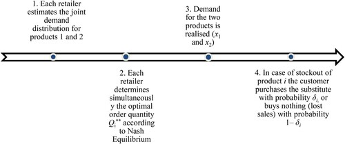
Here, in line with Koren, Perlman, and Shnaiderman (2022), we consider a scenario with two substitutable products, but in this case, each product is offered by a different (competing) retailer. In the competitive scenario, the retailers both order their inventory simultaneously, prior to the start of the selling period (i.e. before demand realisation). Each retailer i aims to order the inventory level Q_i that maximises his or her expected profit, defined below. The sequence of events is summarised in Figure 2.

Figure 2. Sequence of events for competitive setting.

Overview of the competitive setting's events in a timeline. In the first event, a joint demand distribution is estimated and in the last event, the customer makes a purchase or not.

3.2.1. Profit outcomes for different values of inventory and demand

As in the centralised case, we first identify four general profit outcome scenarios for specific values of the inventory levels Q₁ and Q₂, defined in relation to the random demand levels X₁ and X₂.

1. If X₁≤ Q₁ and X₂≤ Q₂, each customer purchases the product that he or she prefers, and the corresponding profit for retailer i is (13) $\begin{array}{r}{\pi }_i(Q_i,X_i)=(p_i-s_i)X_i-(c_i-s_i)Q_i,iϵ\{1,2\}\end{array}$(13)

2. If X₂> Q₂ and X₁≤ Q₁–δ₂(X₂ – Q₂), then retailer 2’s inventory does not meet the demand for product 2, whereas retailer 1’s inventory level satisfies both the demand for product 1 and the demand among customers who prefer product 2 yet found that it was unavailable and are willing to buy product 1 instead. Thus, each retailer’s profit is as follows: $\begin{array}{rl}& {\pi }_1(Q_1,X_1)=(p_1-s_1)[X_1+{\delta }_2(X_2-Q_2)]\\ & \phantom{{\pi }_1(Q_1,X_1)=}-(c_1-s_1)Q_1\end{array}$ (14) $\begin{array}{rl}& {\pi }_2(Q_2,X_2)=p_2{Q}_2-c_2{Q}_2\end{array}$(14)

3. According to the same logic, if X₁ > Q₁ and X₂ ≤ Q_{2 –} δ₁(X₁ – Q₁), then $\begin{array}{rl}{\pi }_1(Q_1,X_1)& =p_1{Q}_1-c_1{Q}_1\end{array}$ (15) $\begin{array}{rl}{\pi }_2(Q_2,X_2)& =(p_2-s_2)[X_2+{\delta }_1(X_1-Q_1)]\\ & -(c_2-s_2)Q_2.\end{array}$(15)

4. Otherwise, all the inventory is sold and the profit of retailer i is equal to (16) ${\pi }_i(Q_i,X_i)=p_i{Q}_i-c_i{Q}_i,iϵ\{1,2\}\text{.}$(16)

3.1.2. Expected profit maximisation

Let Z_i(Q_i| Q_3-i) denote the total expected profit of retailer i, given Q_3-i. According to (13)–(16), Z₁ and Z₂ can be expressed as follows: (17) $\begin{array}{rl}& Z_1(Q_1|Q_2)\\ & =\text{E}[{\pi }_1(Q_1,Q_2,X_1,X_2)]\\ & ={\int }_0^{\mathrm{\infty }}{\int }_0^{\mathrm{\infty }}{\pi }_1(Q_1,Q_2,x_1,x_2)f(x_1,x_2)d{x}_{2}d{x}_1\\ & ={\int }_0^{Q_1}[{\int }_0^{Q_2}((p_1-s_1)x_1+s_1{Q}_1)f(x_1,x_2)d{x}_2\\ & +{\int }_{Q_2}^{Q_2+\frac{Q_1-x_1}{{\delta }_2}}[(p_1-s_1)(x_1+{\delta }_2(x_2-Q_2))+s_1{Q}_1]\\ & \times f(x_1,x_2)d{x}_2+{\int }_{Q_2+\frac{Q_1-x_1}{{\delta }_2}}^{\mathrm{\infty }}{p}_1{Q}_{1}f(x_1,x_2)d{x}_2\phantom{{\int }_0^{000}}]d{x}_1\\ & +{\int }_{Q_1}^{\mathrm{\infty }}{\int }_0^{\mathrm{\infty }}{p}_1{Q}_{1}f(x_1,x_2)d{x}_{2}d{x}_1-c_1{Q}_1\end{array}$(17) and (18) $\begin{array}{rl}& Z_2(Q_2|Q_1)\\ & =\text{E}[{\pi }_2(Q_1,Q_2,X_1,X_2)]\\ & ={\int }_0^{\mathrm{\infty }}{\int }_0^{\mathrm{\infty }}{\pi }_2(Q_1,Q_2,x_1,x_2)f(x_1,x_2)d{x}_{2}d{x}_1\\ & ={\int }_0^{Q_1}[{\int }_0^{Q_2}(p_2-s_2)x_2+s_2{Q}_2)f(x_1,x_2)d{x}_2\\ & +{\int }_{Q_2}^{\mathrm{\infty }}{p}_2{Q}_{2}f(x_1,x_2)d{x}_2]d{x}_1\\ & +{\int }_{Q_1}^{Q_1+\frac{Q_2}{{\delta }_1}}[{\int }_0^{Q_2-{\delta }_1(x_1-Q_1)}[(p_2-s_2)(x_2+{\delta }_1\\ & \times (x_1-Q_1))+s_2{Q}_2]f(x_1,x_2)d{x}_2\\ & +{\int }_{Q_2-{\delta }_1(x_1-Q_1)}^{\mathrm{\infty }}{p}_2{Q}_{2}f(x_1,x_2)d{x}_2]d{x}_1\\ & +{\int }_{Q_1+\frac{Q_2}{{\delta }_1}}^{\mathrm{\infty }}\left[{\int }_0^{\mathrm{\infty }}{p}_2{Q}_{2}f(x_1,x_2)d{x}_2\right]d{x}_1-c_2{Q}_2.\end{array}$(18) Recall that the two retailers order their products simultaneously, prior to demand realisation. Thus, they set inventory levels Q₁** and Q₂** that maximise their expected profits, according to the following Nash equilibrium: (19) $\begin{array}{r}\{\begin{array}{c}{Q}_1^{\ast \ast }=\underset{Q_1\ge 0}{max}{Z}_1(Q_1|Q_2^{\ast \ast })\\ Q_2^{\ast \ast }=\underset{Q_2\ge 0}{max}{Z}_2(Q_2|Q_1^{\ast \ast }\text{)}.\end{array}\end{array}$(19)

Lemma 3.2:

The functions Z₁(Q₁|Q₂) and Z₂(Q₂|Q₁) are concave in Q₁ and in Q₂, respectively.

Proof

: See Appendix A.

In the following Proposition, it is shown that there is a unique Nash solution for the optimal inventory levels. According to Lemma 3.2, and similarly to the case in Parlar (1988), we have shown in Appendix A (A38) that the derivative of retailer 1’s reaction curve is always strictly smaller than the derivative of retailer 2’s reaction curve.

Proposition 3.6:

There exist unique optimal inventory levels Q₁** > 0 and Q₂** > 0, which are obtained by solving the following equations: (20) $\begin{array}{rl}& {\int }_0^{Q_1^{\ast \ast }}{\int }_0^{Q_2^{\ast \ast }+\frac{Q_1^{\ast \ast }-x_1}{{\delta }_2}}f(x_1,x_2)d{x}_{2}d{x}_1=\frac{p_1-c_1}{p_1-s_1}\\ & {\int }_0^{Q_1^{\ast \ast }+\frac{Q_2^{\ast \ast }}{{\delta }_1}}{\int }_0^{Q_2^{\ast \ast }-{\delta }_1{(x_1-Q_1^{\ast \ast })}^{+}}f(x_1,x_2)d{x}_{2}d{x}_1=\frac{p_2-c_2}{p_2-s_2}\end{array}$(20)

Proof:

See Appendix A.

Proposition 3.6 stipulates that each retailer orders a positive inventory level of his or her product; this proposition makes intuitive sense, given that a retailer cannot make a profit without ordering any inventory of the product s/he sells.

3.2.3. Characterisation of the optimal order quantities as a function of the substitution rates

Proposition 3.7:

For every $i\in \{1,2\}$, the optimal order quantity Q_i** decreases in δ_i and increases in δ_3-i.

Proof:

See Appendix A.

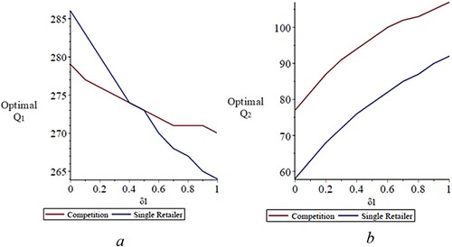
It indeed seems plausible that the optimal order quantity Q_i** should grow when δ_3-i increases, as an increase in δ_3-i implies that more customers of retailer 3 – i are likely to be willing to purchase from retailer i in the event that their preferred product is unavailable. Proposition 3.7 further stipulates that as δ_i increases, Q_i** decreases. This phenomenon results, in part, from the fact that an increase in δ_i triggers an increase in Q_3-i**, which means that fewer customers who prefer product 3 – i will face stockouts and patronise retailer i. Thus, from a practical perspective, the decrease in Q_i** associated with an increase in δ_i should cover the loss of customers who switch from product 3 – i, but it should not be so great that it prevents retailer i from fulfilling the demand of customers who prefer product i. Accordingly, the negative effect of δ_i on the optimal order quantity Q_i** is not expected to be substantial – as we indeed show in our numerical study in subsection 4.3 below (see Figures 3a and 6b).

Figure 3. Effect of δ₁ on the optimal inventory levels Q₁ (a) and Q₂ (b).

A graph showing the value of optimal order quantities for product 1 (3a) and product 2 (3b) as a function of δ1, where the x-axis represents the value of δ1 and the y-axis represents the value of optimal inventory level. Red line indicates competitive settings, and blue line indicates single retailer settings.

3.3. Comparison of the centralised and competitive models

It can be assumed, without loss of generality, that p₁ – c₁ > p₂ – c₂ (i.e. product 1 is more profitable and (8) is always satisfied). In what follows, we show that for small values of δ₁, the optimal inventory level of product 1 in the single-retailer model is greater than that corresponding to the competition model. On the other hand, the optimal inventory level of product 2 is higher in the case of competition.

Proposition 3.8:

When δ₁ is low and close to 0, then Q₁* > Q₁** and Q₂* < Q₂**.

Proof:

See Appendix A.

Proposition 3.8 can be explained according to the following logic. If δ₁ is small and close to 0, then customers who prefer product 1 are generally unwilling to buy product 2 in the event of a stockout of product 1. Recall that we assume that the profit from product 1 is greater than the profit from product 2. Ordering a quantity of product 1 inventory is always preferable; therefore, Q₁ is significantly greater in a single-retailer setting than in a competitive setting, i.e. Q₁* > Q₁**. On the other hand, Q₂ is significantly greater in a competitive setting than in a single retailer (centralised) setting, i.e. Q₂* < Q₂**.

It will now be informally demonstrated that when δ₁ is large and close to 1, the optimal order quantity of product 2 is greater under the competition model than under the centralised model. In turn, the optimal order quantity of product 1 depends on the (fixed) value of δ₂.

Let δ₁= 1 and 0 ≤ δ₂ ≤ (p₂ – c₂)/(p₁-c₁). From (20) and (10) we obtain, respectively, $\begin{array}{rl}& {\int }_0^{Q_1^{\ast \ast }(1,{\delta }_2)}{\int }_0^{Q_2^{\ast \ast }(1,{\delta }_2)+\frac{Q_1^{\ast \ast }(1,{\delta }_2)-x_1}{{\delta }_2}}f(x_1,x_2)d{x}_{2}d{x}_1\\ & =\frac{p_1-c_1}{p_1-s_1}\end{array}$ (21) $\begin{array}{rl}& {\int }_0^{Q_1^{\ast \ast }(1,{\delta }_2)+Q_2^{\ast \ast }(1,{\delta }_2)}{\int }_0^{Q_2^{\ast \ast }(1,{\delta }_2)-{(x_1-Q_1^{\ast \ast }(1,{\delta }_2))}^{+}}f(x_1,x_2)\\ & \times d{x}_{2}d{x}_1=\frac{p_2-c_2}{p_2-s_2}\end{array}$(21) And $\begin{array}{rl}& {\int }_0^{Q_1^{\ast }(1,{\delta }_2)}{\int }_0^{Q_2^{\ast }(1,{\delta }_2)+\frac{Q_1^{\ast }(1,{\delta }_2)-x_1}{{\delta }_2}}f(x_1,x_2)d{x}_{2}d{x}_1\\ & +\frac{p_2-s_2}{p_1-s_1}{\int }_{Q_{1(1,{\delta }_2)}^{\ast }}^{Q_1^{\ast }(1,{\delta }_2)+Q_2^{\ast }(1,{\delta }_2)}{\int }_0^{Q_2^{\ast }(1,{\delta }_2)-(x_1-Q_1^{\ast }(1,{\delta }_2))}\\ & \times f(x_1,x_2)d{x}_{2}d{x}_1=\frac{p_1-c_1}{p_1-s_1}\end{array}$ (22) $\begin{array}{rl}& {\int }_0^{Q_1^{\ast }(1,{\delta }_2)+Q_2^{\ast }(1,{\delta }_2)}{\int }_0^{Q_2^{\ast }(1,{\delta }_2)-{(x_1-Q_1^{\ast }(1,{\delta }_2))}^{+}}f(x_1,x_2)\\ & \times d{x}_{2}d{x}_1+\frac{{\delta }_2(p_1-s_1)}{p_2-s_2}{\int }_0^{Q_1^{\ast }(1,{\delta }_2)}{\int }_{Q_2^{\ast }(1,{\delta }_2)}^{Q_2^{\ast }(1,{\delta }_2)+\frac{Q_1^{\ast }(1,{\delta }_2)-x_1}{{\delta }_2}}\\ & \times f(x_1,x_2)d{x}_{2}d{x}_1=\frac{p_2-c_2}{p_2-s_2}\end{array}$(22) According to (21) and (22), Q₁*(1, δ₂) and Q₂*(1, δ₂) seem to be lower than Q₁**(1, δ₂) and Q₂**(1, δ₂), respectively.

Now let (p₂ – c₂)/(p₁ – c₁) < δ₂ ≤ 1; then Q₂*(1, δ₂)  = 0<Q₂**(1, δ₂), and according to (11), (23) ${\int }_0^{Q_1^{\ast }(1,{\delta }_2)}{\int }_0^{\frac{Q_1^{\ast }(1,{\delta }_2)-x_1}{{\delta }_2}}f(x_1,x_2)d{x}_{2}d{x}_1=\frac{p_1-c_1}{p_1-s_1}$(23) From (23) as well as the first term of (21), Q₁*(1, δ₂) > Q₁**(1, δ₂).

Next, we will consider the case in which δ₂ is small and close to 0, meaning that when product 2 is out of stock, customers are generally unwilling to switch and buy product 1.

Proposition 3.9:

When δ₂ is small and close to 0, then Q₁*< Q₁** and Q₂* > Q₂**.

Proof:

See Appendix A.

When δ₂ is small and close to 0, then customers who prefer product 2 have very low flexibility to buy product 1. The implications of this inflexibility for the products’ optimal order quantities are more significant in the single-retailer model than in the competitive model. Specifically, in a single-retailer setting, Q₂ must be large enough to accommodate almost all the demand for product 2, as customers who prefer this product are likely to be lost. Moreover, Q₂* should satisfy both the original demand for product 2 and the demand among customers who do not receive product 1 and are prepared to buy product 2; therefore, Q₂* > Q₂**.

It will now be demonstrated that when δ₂ exceeds a certain threshold, the optimal inventory level of product 1 is greater in the case of a single retailer than in the competitive setting. For product 2, the opposite holds. Clearly, such a situation would be expected to occur once δ₂ exceeds the threshold (p₂-c₂)/(p₁-c₁), since in this case Q₂* vanishes and Q₁* jumps. However, as presented in Proposition 3.10, these relationships hold even for values of δ₂ that are lower than (p₂ – c₂)/(p₁ – c₁) – but not too small.

Proposition 3.10:

There exists a threshold Δ, 0 < Δ < (p₂-c₂)/(p₁-c₁), such that Q₁* > Q₁** and Q₂* < Q₂** for every Δ <δ₂ ≤ 1 and every δ₁.

Proof:

See Appendix A.

Proposition 3.10 implies that when the substitution rate for a particular product is relatively high – i.e. exceeds a certain threshold – the optimal inventory order size of the alternative product is larger in the case of a single retailer than in a competitive setting.

4. Empirical study

In the second part of our research, we used real-world data to (i) derive the joint sales distribution of two substitutable products; and (ii) obtain concrete insights regarding the ways in which the optimal inventory levels and expected profits are affected by the values of the model parameters (through a sensitivity analysis). To obtain our data, we collaborated with an online fast fashion retailer that sells clothing and footwear for women and men. The retailer provided us with daily-level data regarding a year’s worth of sales for a sneaker that was available in two colours. To protect the retailer’s anonymity, we do not present our collected data set in full. We further note that, as elaborated in what follows, the data set used in our analysis excludes several days with high volatility in sales, corresponding to major holidays (e.g. New Year's Day and Black Friday).

4.1. Sales data

Our data set included the daily sales for each of the two sneaker versions (colours), denoted product 1 and product 2, for the period between January 2020 and December 2020. We were also provided with the products’ unit prices and order costs. Table 1 presents summary statistics for the sales data, excluding major holidays. On average, product 1 sold 776.69 units per day, and product 2 sold 275.48 units per day. The median and mode are equal and very close to the mean for each colour.

Table 1. Summary statistics of sales data (number of product units sold per day).

Product	Mean	Std. deviation	Median	Mode	Minimum	Maximum
Product 1	776.69	329.89	750	750	75	1825
Product 2	275.48	148.28	267	267	25	950

First, for each of the two products, we conducted Kolmogorov–Smirnov tests (with a level of significance α = 0.05) to determine whether the sales distributions were close to normal. We carried out this test twice for each product. The first time, we included all sales data, including major holidays that usually have high sales volatility (365 days). The second time, we excluded major holidays (using data for 355 days). When the data did not include major holidays, test results indicated that the sales distribution for product 1 was normal (p = 0.077), whereas the distribution of sales for product 2 was not normal (p close to 0), with positive skewness and kurtosis (0.127 and 0.085 respectively). To normalise the data, we took the square root of the sales of product 2 (resulting in a normal distribution, p > 0.05). To ensure comparability of the data for the two products, we also took the square root of the sales of product 1 and reapplied the Kolmogorov–Smirnov (excluding major holidays); we once again obtained a p-value greater than 0.05, indicating a normal distribution (see Appendix B1). Thus, in what follows, we assume that the daily square root sales of product 1 and of product 2 are each normally distributed, with statistics given in Table 2.

Table 2. Summary statistics of sales (number of product units sold per day) after square root transformation.

Product	Mean	Std. deviation	Median	Mode	Minimum	Maximum
Product 1	27.22	6.005	27.38	27.38	8.66	42.72
Product 2	15.985	4.472	16.34	16.34	5	30.82

4.2. Joint demand distribution

We denote by x₁ and x₂ the daily sales of products 1 and 2, respectively. In line with prior models addressing inventory management of (fast) fashion products (e.g. Caro and Gallien 2010; Kamanchi et al. 2020; Lucci, Schiraldi, and Varisco 2016), as well as stockout-based substitution (e.g. Martínez-de-Albéniz and Kunnumkal 2022), we assume that x₁ and x₂ are Poisson-distributed random variables, with time-dependent means. Our aim is to estimate these means as a function of the day of the week and the date in the year. A salient feature of the Poisson distribution is that, for a Poisson-distributed variable X with a mean that is not too small, $\sqrt{X}$ is approximately normally distributed with standard deviation 0.5 (see Lemma 3 in Appendix B1). Since sales may occur in batches, the constant standard deviation may be higher. As will be seen in what follows, goodness-of-fit tests provide ample justification for our assumption that x₁ and x₂ are Poisson-distributed.

To estimate variables of interest – namely, the standard deviations σ₁ and σ₂, the correlation coefficient ρ, and the time-dependent mean functions μ₁(t) and μ₂(t) of the bivariate normal pair ($\sqrt{x_1},\sqrt{x_2})$ – we fit a periodic function to the square root of the sales, based on a yearly and a daily period. Specifically, we used a multiple linear regression model with trigonometric elements. The explanatory variables (predictors) were sine and cosine variables corresponding to the period of one week, and sine and cosine variables corresponding to the period of one year.

The coefficients for the two regression models are presented in Appendix B2. For product 1 (Table B.2.1 in Appendix B2), the predictors explain 51% of the variance in (the square root of the) sales (Multiple R = 0.71, R² = 0.51, Adjusted R² = 0.51). We then obtain: (24) $\begin{array}{rl}{\mu }_1& =27.06+0.952\times \sin (B_{1}t)+0.783\times \cos (B_{1}t)\\ & +2.547\times \sin (B_{2}t)-5.433\times \cos (B_{2}t),\end{array}$(24) where $B_1=\frac{2\pi }{7}$, $B_2=\frac{2\pi }{355}$, and t is the time measured in days.

For product 2 (Table B.2.2 in Appendix B2), all predictors together explain 45% of the sales variation (Multiple R = 0.67, R² = 0.45, Adjusted R² = 0.44). We then obtain: (25) $\begin{array}{rl}{\mu }_2& =15.89-0.383\times \sin (B_{1}t)+0.545\times \cos (B_{1}t)\\ & +2.35\times \sin (B_{2}t)-3.497\times \cos (B_{2}t),\end{array}$(25) where $B_1=\frac{2\pi }{7}$, $B_2=\frac{2\pi }{355}$ and t is the time measured in days.

The values µ_i (for each product i) obtained by the above regressions ((24)-(25)) are depicted in Table 3.

Table 3. Parameters for model.

	Expected value (μ)	St. deviation (σ)	Unit selling price (p)	Order cost (c)	Salvage value (s)
Product 1	20.17	4.19	$79	$66	$0
Product 2	12.29	3.31	$71	$61	$0

Next, we analysed the residuals (i.e. actual transformed sales minus µ_i, $\sqrt{X_i}-{\mu }_i$). For each product, we performed a Kolmogorov–Smirnov test (at the level of significance α = 0.05), and found that the distribution of the residuals was adequately normal (p-value greater than 0.05). Then, we performed the Jarque-Bera (J-B) test to test joint normality (Jarque and Bera 1980). In our case, the J-B value for product 1 was 0.272, and the value for product 2 was 0.21 (see Appendix B1, Figure B1.3). As the null hypothesis in the J-B test was not rejected, we proceeded to evaluate the empirical covariance matrix of the residuals (2 columns and 355 rows), to estimate σ₁ and σ₂. Specifically, for product 1 we obtained σ₁ = 4.19; and for product 2 we obtained σ₂ = 3.31. The value of the correlation coefficient for the joint distribution, denoted by ρ, is 0.5689. Because fast fashion products are characterised by a short life cycle and short storage life, zero salvage value can be assumed (Chen, Tian, and Yang 2014). These data are summarised in Table 3. ¹

4.3. Sensitivity analysis

In this section, we apply our models to the data obtained from the retailer, including the parameter values derived in the previous section (see Table 3). Specifically, we explore how the optimal inventory level for each product, as well as the retailers’ expected profits, are affected by adjustments to the following three parameters: the probability of substitution (δ), the unit selling price (p), and the correlation coefficient (ρ(, which affects the joint probability distribution function.

According to Table 3, p₁ is larger than p₂, and the first two terms of (7) are satisfied for every 0 ≤ δ₁ ≤ 1 and 0 ≤ δ₂ ≤ 0.9. Therefore, it is assumed that δ₂ does not exceed 0.9 and that δ₁δ₂ is lower than or equal to 0.5, so that problem (6) is concave. Also, p₁ – c₁ > p₂ – c₂, that is, condition (8) is satisfied for every 0 ≤ δ₁ ≤ 1, whereas (9) is met only if 0 ≤ δ₂ ≤ 0.769. Consequently, for the single-retailer model, the optimal inventory level of product 1 is always positive, whereas that of product 2 disappears under the single-retailer model if δ₂ exceeds 0.769.

4.3.1. The impact of stockout-based substitution rate on optimal inventory levels and profits

First, we examine the case in which δ₂ is fixed at 0.5, and the value of δ₁ is varied between 0 and 1 (recall that a higher value of δ₁ indicates higher willingness of customers who prefer product 1 to buy product 2 in the event of an inventory shortage). Figure 3 presents the optimal inventory levels of product 1 (Figure 3a) and of product 2 (Figure 3b), in both the centralised and competitive settings, as functions of δ₁.

In accordance with Propositions 3.3 and 3.7, we observe that in both the centralised and competitive cases, the optimal inventory level of product 1 (Q₁* or Q₁**) decreases in δ₁ (Figure 3a), and the optimal inventory level of Q₂ (Q₂* or Q₂**) increases in δ₁. In other words, as δ₁ increases, increasing the inventory level of product 1 is not profitable. Instead, it is preferable to increase the inventory level of product 2. Notably, Q₁ decreases more steeply in a single-retailer setting than in a competitive setting, as is mentioned in the discussion following Proposition 3.7 above.

We further observe that, in accordance with Proposition 3.8, when δ₁ is small, the optimal order quantity for product 1 is lower in a competitive setting (Q₁**) than in a centralised setting (Q₁*). Yet, when δ₁ is large, the opposite is the case. For product 2, however, the optimal inventory level of product 2 is always higher in a competitive setting than in a centralised setting.

Figure 4 shows the total optimal inventory level (Q₁ + Q₂) for each setting, as a function of δ₁. We observe that the total optimal inventory level increases in both settings, but that it increases more steeply in the competitive setting, eventually surpassing the optimal inventory level in the single-retailer setting.

Figure 4. Effect of δ₁ on the total optimal inventory level (Q₁ + Q₂).

A graph showing the value of sum of optimal order quantities for product 1 and product 2 as a function of δ1, where the x-axis represents the value of δ1 and the y-axis represents the value of optimal inventory level. Red line indicates competitive settings, and blue line indicates single retailer settings.

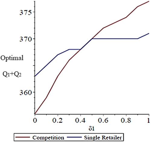
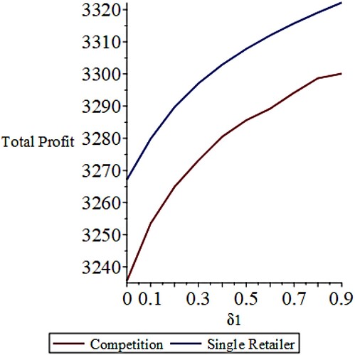
Figure 5 shows the retailers’ expected profits as a function of δ₁. The single retailer's total profit is compared to the sum of the profits of the competitive retailers. The single retailer's expected profit increases from 3270 to 3320 (slightly more than 1.5%) as δ₁ increases to 0.9 (according to Proposition 3.4). The total expected profit of the two competitive retailers increases from 3230 to 3300 (slightly more than 2%).

Figure 5. Effect of δ₁ on the profits of the retailer(s). The graph for the competition scenario represents the sum of profits for the two retailers.

A graph showing the value of total retailer's profit for product 1 and product 2 as a function of δ1, where the x-axis represents the value of δ1 and the y-axis represents the value of total profit. Red line indicates competitive settings, and blue line indicates single retailer settings.

Next, we carry out a similar analysis for the case in which δ₁ is fixed at 0.5, and the value of δ₂ is varied between 0 and 0.9. Figure 6 shows the optimal order quantities. We observe that Q₁* and Q₁** increase in δ₂ (Figure 6a), whereas Q₂* and Q₂** decrease (Figure 6b), as stated in Propositions 3.3 and 3.7. In this case, the increase or decrease in the single-retailer setting is significantly steeper than in the competitive setting. In particular, while Q₂* drops from 105 to 0, the effect of δ₂ on Q₂**, is negligible (that order quantity decreases from 101 to 98).

Figure 6. Effect of δ₂ on the optimal inventory levels Q₁ (a) and Q₂ (b).

A graph showing the value of optimal order quantities for product 1 (6a) and product 2 (6b) as a function of δ2, where the x-axis represents the value of δ2 and the y-axis represents the value of optimal inventory level. Red line indicates competitive settings, and blue line indicates single retailer settings.

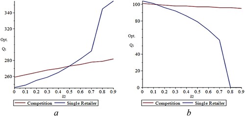
We further observe that, in accordance with Proposition 3.9, when δ₂ is small, Q₁** > Q₁* and Q₂* > Q₂**. This relationship is reversed when δ₂ is close to 1, as Q₂* vanishes and Q₁* increases. The optimal inventory levels of the two models intersect at δ₂= 0.5 for product 1 and δ₂= 0.15 for product 2.

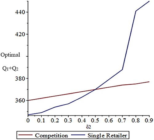
Figure 7 shows that that total inventory (the sum of the optimal values of Q₁ + Q₂) increases more steeply in δ₂ in the single-retailer setting than in the competitive setting, in line with the steep increase in Q₁* observed in Figure 6a.

Figure 7. Effect of δ₂ on the total optimal inventory level (Q₁ + Q₂).

A graph showing the value of sum of optimal order quantities for product 1 and product 2 as a function of δ2, where the x-axis represents the value of δ2 and the y-axis represents the value of total optimal inventory level. Red line indicates competitive settings, and blue line indicates single retailer settings.

The results above are compatible with the reasoning that, since the profit from product 1 is greater than that of product 2, when δ₂ increases (i.e. increasing customers’ flexibility to buy product 1), a retailer who sells product 1 benefits from increasing the inventory level of that product.

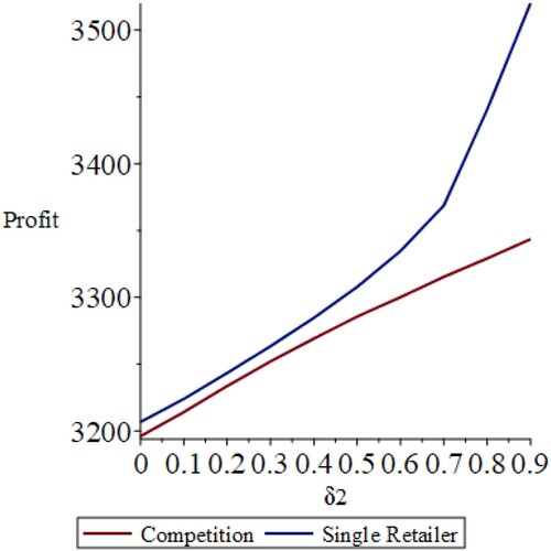
Regarding the retailers’ expected profit, Figure 8 shows that the total expected profit of the two competitive retailers increases in δ₂ from 3200 to 3350 (almost 4.7%). In a single-retailer setting, the expected profit from both products increases to a greater extent – from 3200 to 3500 (slightly more than 9.3%) as δ₂ increases to 0.9.

Figure 8. Effect of δ₂ on the profits of the retailer(s). The graph for the competition scenario represents the sum of profits for the two retailers.

A graph showing the value of total retailer's profit for product 1 and product 2 as a function of δ2, where the x-axis represents the value of δ2 and the y-axis represents the value of total profit. Red line indicates competitive settings, and blue line indicates single retailer settings.

4.3.2. The impact of unit selling price ratio on optimal inventory levels

In this section we examine how the optimal inventory levels are affected by an increase in the unit selling price ratio (p₁/p₂). In order to maintain the ratio between the unit selling price (p) and order cost (c), we assume that a change in the unit selling price is accompanied by a corresponding change in the order cost. The optimal inventory levels of Q₁ and Q₂, are presented in Figure 9a,b, respectively.

Figure 9. Effects of p₁/p₂ on the optimal inventory levels for Q₁ (a) and Q₂ (b).

A graph showing the value of optimal order quantities for product 1 (9a) and product 2 (9b) as a function of the ratio between unit selling prices p1/p2, where the x-axis represents the value of p1/p2 and the y-axis represents the value of optimal inventory level. Red line indicates competitive settings, and blue line indicates single retailer settings.

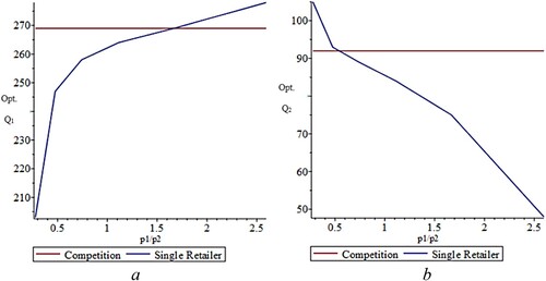
According to Proposition 3.6, in a competitive setting, the optimal inventory level of Q_i depends only on c_i/p_i. Given our assumption that c_i/p_i remains constant, it is clear that in a competitive setting, Q₁** and Q₂** do not change as a function of p₁/p₂. In a single-retailer setting, however, according to Proposition 3.1, Q_i* depends on c_i/p_i and on p_3-i/p_i. Consequently, the inventory levels change as a function of p₁/p₂. Q₁* increases in p₁/p₂, whereas Q₂* decreases.

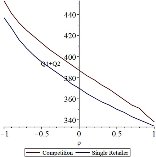
4.3.3. The impact of the correlation coefficient on optimal inventory levels

The correlation coefficient ρ is an indication of the extent to which demand for the two products is correlated, in the absence of substitution.

Figures 10 and 11 show, respectively, how the optimal inventory levels and the total inventory level respond to the value of the correlation coefficient. We observe that when the correlation coefficient is positive, the optimal inventory levels of both products are low, due to the risk of having low demand for both products simultaneously. On the other hand, this situation has low probability when the correlation coefficient is negative, and therefore the inventory levels are high.

Figure 10. Effect of correlation coefficient ρ on the inventory levels of Q₁ (a) and Q₂ (b).

A graph showing the value of optimal order quantities for product 1 (11a) and product 2 (11b) as a function of correlation coefficient ρ, where the x-axis represents the value of correlation coefficient ρ and the y-axis represents the value of optimal inventory level. Red line indicates competitive settings, and blue line indicates single retailer settings.

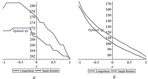
Figure 11. Effect of correlation coefficient ρ on the total optimal inventory (Q₁ + Q₂).

A graph showing the value of sum of optimal order quantities for product 1 and product 2 as a function of correlation coefficient ρ, where the x-axis represents the value of correlation coefficient ρ and the y-axis represents the value of total optimal inventory level. Red line indicates competitive settings, and blue line indicates single retailer settings.

5. Conclusion and managerial implications

This work addressed retailers’ inventory decisions for substitutable products, focusing on the fashion industry, where demand is uncertain, yet consumers are often willing to accept product substitutes when their preferred products are out of stock (e.g. select the same garment in a different colour). We developed single-period models to describe a market in which two substitutable products are sold, and retailers must select the inventory amounts that maximise their expected profits, under stockout-based substitution. We considered both a centralised setting, in which a single retailer offers both products, and a competitive setting, in which each product is offered exclusively by a different retailer.

In both cases, we proved that the objective functions are concave so that a unique optimal solution exists. Moreover, for the centralised setting, we identified conditions under which the retailer benefits from maintaining positive inventory levels for both products, as well as conditions under which it is preferable to stock only one type of product. In each case, we analytically described how the optimal order quantity and expected profits respond to changes in the parameter values, including the substitution rate (i.e. consumers’ willingness to substitute one product for another in the event of a stockout) and product unit prices and costs. We also compared the two settings, identifying scenarios, for example, in which the optimal order quantity for a particular product in the single-retailer setting exceeds that in the competitive setting, or vice versa.

We enriched our model with data from an online apparel retailer regarding the sales of two substitutable products (sneakers in two different colours); these data enabled us to estimate the demand distribution. We subsequently conducted analyses, grounded in empirical data, to derive concrete insights regarding the sensitivity of optimal inventory levels and expected profits to specific parameter values.

Together, the analytical and empirical components of our work converge to the following managerial insights: (i) Optimal inventory levels are significantly affected by customers’ willingness to substitute one product for another in the event that their preferred product is out of stock. Indeed, in the case of a single retailer (centralised setting), there are conditions in which it may be preferable to stock only one type of product (specifically, the more profitable of the two), if consumers are sufficiently willing to substitute that product for their preferred product. In the case of two competing retailers, however, the optimal order quantity for each product is always positive, given that each retailer only offers one type of product, and thus a lack of stock means a lack of profit. (ii) Similarly, when customers’ willingness to compromise is greater, retailers’ expected profit is higher – under both centralised and competitive settings. (iii) Comparing between the two settings, we find that when customers’ flexibility regarding a particular product is low, the optimal inventory order size of that product is larger in the case of a single retailer than in the competitive setting. Conversely, the inventory order size of the other product is larger in the competitive setting than in the centralised case. (iv) When the demand levels for the two products are highly correlated, the optimal inventory levels of both products are low, due to the risk of having very low demand for both products simultaneously.

Future research might extend our work in several ways. One possibility would be to account for lost sales – in which a retailer who runs out of a particular product incurs a penalty when customers leave without making a purchase (and, when possible, buy the product elsewhere). In this case, the solution becomes more complicated, because the objective function depends on the arrival rates of the customers who are interested in buying the product (see preliminary formulation of the model in Appendix C). Another option is to extend our work to encompass a multi-product model that is dynamically solved during a number of different periods (with leftover inventory from previous periods). Such a model would more realistically capture retailers’ decisions in practice, which encompass large numbers of products that may be saleable over multiple periods (e.g. with markdowns on older products as new products enter the market).

Acknowledgements

The authors would like to thank Isaac Meilijson for his help in estimating the joint demand and the three anonymous reviewers for their constructive comments and suggestions which have significantly improved the paper.

Data availability statement

Data available on request from the authors.

Disclosure statement

No potential conflict of interest was reported by the author(s).

Additional information

Funding

This research was partially supported by the Israel Science Foundation (grant number 1898/21).

Notes on contributors

Michal Koren

Michal Koren holds a Ph.D. and an M.A. in Industrial Management, both from the Department of Management, Bar-Ilan University in Israel, and a B.Sc. in Industrial Engineering and Management from Shenkar- Engineering. Design. Art. Currently, she is a faculty member and deputy dean at the School of Industrial Engineering and Management at Shenkar- Engineering. Design. Art. Her research interests include Operations Research, Supply Chain, Machine Learning and Artificial Intelligence.

Yael Perlman

Yael Perlman is an Associate Professor of Operations Management in the Department of Management at Bar-Ilan University, Israel. She holds a BSc in Mathematics (TAU) an MBA in Operations Research (TAU) and a PhD in Industrial Engineering (BGU). Yael Perlman develops game theory-based models and queuing theory-based models to investigate strategic decisions of the supply chain members and the effect of intra-supply chain competition on the overall supply chain performance. Her papers have been published in some of the leading journals of Supply Chain Management and Operations Management.

Matan Shnaiderman

Matan Shnaiderman received M.S. and Ph.D. degrees in the Department of Mathematics, Bar-Ilan University in Israel. He is currently Senior Lecturer at the Department of Management, Bar-Ilan University. His research interests include supply-chain and inventory management, information sharing, public transit, frequency setting, energy production and stochastic dynamic programming.

Notes

1 Since we do not have data from two rival retailers, we used the data from Table 3 in the sensitivity analysis performed in the next subsection as a scenario analysis.

References

- Achamrah, F. E., F. Riane, and S. Limbourg. 2022. “Solving inventory routing with transshipment and substitution under dynamic and stochastic demands using genetic algorithm and deep reinforcement learning.” International Journal of Production Research, 60 (20), 6187–6204.
- Ambilkar, P., V. Dohale, A. Gunasekaran, and V. Bilolikar. 2022. “Product Returns Management: A Comprehensive Review and Future Research Agenda.” International Journal of Production Research 60 (12): 3920–3944. https://doi.org/10.1080/00207543.2021.1933645
- Besbes, O., and D. Sauré. 2016. “Product Assortment and Price Competition Under Multinomial Logit Demand.” Production and Operations Management 25 (1): 114–127. https://doi.org/10.1111/poms.12402
- Caro, F., and J. Gallien. 2010. “Inventory Management of a Fast-Fashion Retail Network.” Operations Research 58 (2): 257–273. https://doi.org/10.1287/opre.1090.0698
- Chen, B., and X. Chao. 2020. “Dynamic Inventory Control with Stockout Substitution and Demand Learning.” Management Science 66 (11): 5108–5127. https://doi.org/10.1287/mnsc.2019.3474
- Chen, W., Tian, Y., & Yang, Y. X. (2014, August). “Decentralized and Centralized Supply Chain Decision-Making of Low Salvage Value Products with Price-postponement Strategy.” In 2014 International Conference on Management Science & Engineering 21th Annual Conference Proceedings, 345–350. IEEE.
- Choi, T. M., and S. Guo. 2018. “Responsive Supply in Fashion Mass Customisation Systems with Consumer Returns.” International Journal of Production Research 56 (10): 3409–3422. https://doi.org/10.1080/00207543.2017.1292065
- Dong, Z. S., W. Chen, Q. Zhao, and J. Li. 2020. “Optimal Pricing and Inventory Strategies for Introducing a new Product Based on Demand Substitution Effects.” Journal of Industrial & Management Optimization 16 (2): 725–739. https://doi.org/10.3934/jimo.2018175
- DuBreuil, M., and S. Lu. 2020. “Traditional vs. big-Data Fashion Trend Forecasting: An Examination Using WGSN and EDITED.” International Journal of Fashion Design, Technology and Education 13 (1): 68–77. https://doi.org/10.1080/17543266.2020.1732482
- Ergin, E., M. Gümüş, and N. Yang. 2022. “An Empirical Analysis of Intra-Firm Product Substitutability in Fashion Retailing.” Production and Operations Management 31 (2): 607–621. https://doi.org/10.1111/poms.13569
- Goyal, V., R. Levi, and D. Segev. 2016. “Near-optimal Algorithms for the Assortment Planning Problem Under Dynamic Substitution and Stochastic Demand.” Operations Research 64 (1): 219–235. https://doi.org/10.1287/opre.2015.1450
- Gupta, V. K., Q. U. Ting, and M. K. Tiwari. 2019. “Multi-period Price Optimization Problem for Omnichannel Retailers Accounting for Customer Heterogeneity.” International Journal of Production Economics 212: 155–167. https://doi.org/10.1016/j.ijpe.2019.02.016
- Gümüş, M., P. Kaminsky, and S. Mathur. 2016. “The Impact of Product Substitution and Retail Capacity on the Timing and Depth of Price Promotions: Theory and Evidence.” International Journal of Production Research 54 (7): 2108–2135. https://doi.org/10.1080/00207543.2015.1108536
- Hammami, R., E. Asgari, Y. Frein, and I. Nouira. 2022. “Time-and Price-Based Product Differentiation in Hybrid Distribution with Stockout-Based Substitution.” European Journal of Operational Research 300 (3): 884–901. https://doi.org/10.1016/j.ejor.2021.08.042
- Ho, W., T. Zheng, H. Yildiz, and S. Talluri. 2015. “Supply Chain Risk Management: A Literature Review.” International Journal of Production Research 53 (16): 5031–5069. https://doi.org/10.1080/00207543.2015.1030467
- Honhon, D., V. Gaur, and S. Seshadri. 2010. “Assortment Planning and Inventory Decisions Under Stockout-Based Substitution.” Operations Research 58 (5): 1364–1379. https://doi.org/10.1287/opre.1090.0805
- Hübner, A. 2017. “A Decision Support System for Retail Assortment Planning.” International Journal of Retail & Distribution Management. 45 (7/8): 808–825. https://doi.org/10.1108/IJRDM-09-2016-0166.
- Jarque, C. M., and A. K. Bera. 1980. “Efficient Tests for Normality, Homoscedasticity and Serial Independence of Regression Residuals.” Economics Letters 6 (3): 255–259. https://doi.org/10.1016/0165-1765(80)90024-5
- Kamanchi, C., G. A. Kumar, N. Sundaram, and C. Bandi. 2020. “An Application of Newsboy Problem in Supply Chain Optimisation of Online Fashion E-Commerce.” arXiv preprint arXiv:2007.02510.
- Ko, E., J. P. Costello, and C. R. Taylor. 2019. “What is a Luxury Brand? A new Definition and Review of the Literature.” Journal of Business Research 99: 405–413. https://doi.org/10.1016/j.jbusres.2017.08.023
- Koren, M., Y. Perlman, and M. Shnaiderman. 2022. “Inventory Management Model for Stockout Based Substitutable Products.” IFAC-PapersOnLine 55 (10): 613–618. https://doi.org/10.1016/j.ifacol.2022.09.467
- Kök, A. G., M. L. Fisher, and R. Vaidyanathan. 2015. “Assortment Planning: Review of Literature and Industry Practice.” In Retail Supply Chain Management. International Series in Operations Research & Management Science, edited by N. Agrawal and S. Smith, vol. 223, 175–236. New York: Springer.
- Li, M., and T. Li. 2018. “Consumer Search, Transshipment, and Bargaining Power in a Supply Chain.” International Journal of Production Research 56 (10): 3423–3438. https://doi.org/10.1080/00207543.2017.1326644
- Li, S., L. X. Lu, S. F. Lu, and S. Huang. 2023. “Estimating the Stockout-Based Demand Spillover Effect in a Fashion Retail Setting.” Manufacturing & Service Operations Management 25 (2): 468–488.
- Loureiro, A. L., V. L. Miguéis, and L. F. da Silva. 2018. “Exploring the use of Deep Neural Networks for Sales Forecasting in Fashion Retail.” Decision Support Systems 114: 81–93. https://doi.org/10.1016/j.dss.2018.08.010
- Lucci, G., M. M. Schiraldi, and M. Varisco. 2016. “Fashion Luxury Retail Supply Chain: Determining Target Stock Levels and Lost Sale Probability.” In 21st Summer School Francesco Turco 2016 (Vol. 13, pp. 192–197). AIDI-Italian Association of Industrial Operations Professors.
- Martínez-de-Albéniz, V., and S. Kunnumkal. 2022. “A Model for Integrated Inventory and Assortment Planning.” Management Science 68 (7): 5049–5067. https://doi.org/10.1287/mnsc.2021.4149
- Ovezmyradov, B., and H. Kurata. 2019. “Effects of Customer Response to Fashion Product Stockout on Holding Costs, Order Sizes, and Profitability in Omnichannel Retailing.” International Transactions in Operational Research 26 (1): 200–222. https://doi.org/10.1111/itor.12511
- Parlar, M. 1988. “Game Theoretic Analysis of the Substitutable Product Inventory Problem with Random Demands.” Naval Research Logistics (NRL) 35 (3): 397–409. https://doi.org/10.1002/1520-6750(198806)35:3<397::AID-NAV3220350308>3.0.CO;2-Z
- Perlman, Y. 2019. “Inventory Levels of Two Stockout-Based Substitutable Products Under Centralized and Competitive Settings.” IFAC-PapersOnLine 52 (13): 1450–1454. https://doi.org/10.1016/j.ifacol.2019.11.403
- Ren, S., H. L. Chan, and T. Siqin. 2020. “Demand Forecasting in Retail Operations for Fashionable Products: Methods, Practices, and Real Case Study.” Annals of Operations Research 291 (1-2): 761–777. https://doi.org/10.1007/s10479-019-03148-8
- Schlapp, J., and M. Fleischmann. 2018. “Multiproduct Inventory Management Under Customer Substitution and Capacity Restrictions.” Operations Research 66 (3): 740–747. https://doi.org/10.1287/opre.2017.1690
- Shen, B., H. L. Chan, P. S. Chow, and K. A. Thoney-Barletta. 2016. “Inventory Management Research for the Fashion Industry.” International Journal of Inventory Research 3 (4): 297–317. https://doi.org/10.1504/IJIR.2016.082325
- Shin, H., S. Park, E. Lee, and W. C. Benton. 2015. “A Classification of the Literature on the Planning of Substitutable Products.” European Journal of Operational Research 246 (3): 686–699. https://doi.org/10.1016/j.ejor.2015.04.013
- Shokouhyar, S., S. Shokoohyar, N. Raja, and V. Gupta. 2021. “Promoting Fashion Customer Relationship Management Dimensions Based on Customer Tendency to Outfit Matching: Mining Customer Orientation and Buying Behaviour.” International Journal of Applied Decision Sciences 14 (1): 1–23. https://doi.org/10.1504/IJADS.2021.112932
- Singh, D., and A. Verma. 2018. “Inventory Management in Supply Chain.” Materials Today: Proceedings 5 (2): 3867–3872. https://doi.org/10.1016/j.matpr.2017.11.641
- Transchel, S. 2017. “Inventory Management Under Price-Based and Stockout-Based Substitution.” European Journal of Operational Research 262 (3): 996–1008https://doi.org/10.1016/j.ejor.2017.03.075
- Wan, M., Y. Huang, L. Zhao, T. Deng, and J. C. Fransoo. 2018. “Demand Estimation Under Multi-Store Multi-Product Substitution in High Density Traditional Retail.” European Journal of Operational Research 266 (1): 99–111https://doi.org/10.1016/j.ejor.2017.09.014
- Wang, Q., and B. Zhang. 2021. “A Guarantee Credit Model with Substitutable Product Competition.” International Journal of Production Research 59 (22): 6919–6940. https://doi.org/10.1080/00207543.2020.1830195
- Wang, S., H. Zhang, F. Chu, and L. Yu. 2022. “A Relax-and-fix Method for Clothes Inventory Balancing Scheduling Problem.” International Journal of Production Research, 1–20. https://doi.org/10.1080/00207543.2022.2145517
- Wen, X., T. M. Choi, and S. H. Chung. 2019. “Fashion Retail Supply Chain Management: A Review of Operational Models.” International Journal of Production Economics 207: 34–55. https://doi.org/10.1016/j.ijpe.2018.10.012
- Yamazaki, T., K. Shida, and T. Kanazawa. 2016. “An Approach to Establishing a Method for Calculating Inventory.” International Journal of Production Research 54 (8): 2320–2331. https://doi.org/10.1080/00207543.2015.1076179
- Zeppetella, L., E. Gebennini, A. Grassi, and B. Rimini. 2017. “Optimal Production Scheduling with Customer-Driven Demand Substitution.” International Journal of Production Research 55 (6): 1692–1706. https://doi.org/10.1080/00207543.2016.1223895
- Zhang, X., M. Yang, J. Su, W. Yang, and K. Qiu. 2020. “Research on Product Color Design Decision Driven by Brand Image.” Color Research & Application 45 (6): 1202–1216. https://doi.org/10.1002/col.22540
- Zhao, Y., and X. Zhao. 2016. “How a Competing Environment Influences Newsvendor Ordering Decisions.” International Journal of Production Research 54 (1): 204–214. https://doi.org/10.1080/00207543.2015.1034330