A machine learning study to improve the reliability of project cost estimates

Abstract

Project managers need reliable predictive analytics tools to make effective project intervention decisions throughout the project life cycle. This study uses Machine learning (ML) to enhance the reliability in project cost forecasting. A XGBoost forecasting model is developed and computational experiments are conducted using real data of 110 projects representing 1268 cost data points. The developed model performs better than some Earned value management (EVM), ML (Random forest, Support vector regression, LightGBM, and CatBoost), and non-linear growth (Gompertz and Logistic) models. The model produces more accurate estimates at the early, middle, and late stages of the project execution, allowing for early warning signals for more effective cost control. In addition, it shows more accurate estimates in most projects tested, suggesting consistency when repeatedly used in practice. Project forecasting studies mainly used ML to estimate the project duration; a few ML studies estimated the project cost at the project’s conceptual stage. This study uses real data and EVM metrics, proposing an effective XGBoost model for forecasting the cost throughout the project life cycle.

KEYWORDS:

• Cost forecasting
• earned value management
• machine learning
• non-linear growth model
• project monitoring and control
• The XGBoost model

1. Introduction

Today, in the new era of rapid technological developments, managers need to make quick decisions that deal with the uncertainties and complexities of dynamic business environments. Computational intelligence techniques of Artificial intelligence (AI) and data analytics can improve managerial decision-making under uncertainty. Literature on the use of these techniques has been rapidly growing recently. For example, researchers that work on operations management have been using them to solve various forecasting, inventory planning, revenue management, and transportation problems (Choi, Wallace, and Wang 2018). In project management, there are many application areas and potential benefits of using data analytics and AI (Munir 2019; Ong and Uddin 2020), but the literature on the applications is scant. This scarcity can be linked to each project being unique, and predicting the project outcomes using limited historical data is ineffective. However, in any industry, many activities of different projects are common.

Nevertheless, data analytic tools can aid project managers in various ways. To give a specific example, they can use them to identify various project risks, predict their probabilities and impacts more accurately, and prepare risk plans accordingly. Alternatively, in product design projects, they can quickly analyse customer feedback and incorporate it by supporting these tools. We refer to Bakici, Nemeh, and Hazir (2021) and Ulusoy and Hazır (2021) for a review of specific application areas.

Among several application areas of AI in project management, we address project cost forecasting and aim to predict the total project cost accurately. In addition to the accuracy of cost forecasting, we also evaluate the timeliness of forecasting. It is a criterion to evaluate the reliability of the prediction model when it provides more accurate estimates earlier in the project life (Kim, Wells, and Duffey 2003; Teicholz 1993). Because the cost forecasting method must generate early warnings of cost overruns, in this way, more effective project control decisions can be taken. We use a Machine learning (ML) approach, which includes algorithms to learn from the given data and apply the acquired knowledge for the decision-making process, i.e. cost forecasting in the current study. Several regression techniques, neural networks, decision trees, clustering, and pattern recognition algorithms could be considered techniques of ML. Merhi and Harfouche (2023) discuss adopting and implementing these AI techniques in production systems. Rai et al. (2021) comprehensively review these techniques and applications in manufacturing and Industry 4.0. Rolf et al. (2022) present the applications of reinforcement learning in supply chain management.

ML could be used in projects from the initiation to the closure stages. Bilal and Oyedele (2020) develop a benchmarking system for evaluating the tenders effectively using Big data and Deep learning. Their system allows project contractors to perform a complete analysis of the bids. Elmousalami (2021) also implements ML to support decision-making at the early stages of the projects, specifically in conceptual cost estimations. They integrate uncertainty factors into the models using fuzzy theory. Their results show the performance superiority of ensemble methods, which combine multiple learning algorithms to improve the overall prediction performance. Dahmani, Ben-Ammar, and Jebali (2021) develop a conceptual framework to use ML to schedule projects under uncertainty. Also, risk analysis is an important application area of ML in projects. Owolabi et al. (2020) used big data predictive analytics techniques to study the risk items in public-private partnership projects. They predicted the delays and analysed the project completion risks using five techniques: linear regression, decision tree, random forest, support vector machine, and neural network. They found the technique to show the best predictive performance for forecasting the project delay. Their analysis provided valuable information to project managers to enhance their risk plans. Wauters and Vanhoucke (2016) use decision trees, bagging, random forest, and boosting techniques to predict the project completion time and compare the performance of these techniques. They generate their data for testing, and using this data, they show that all these ML methods have better-predicting capabilities than traditional forecasting methods.

In this study, we use ML for project cost forecasting. Some recent studies suggest using ML in duration and cost forecasting (e.g. Pellerin and Perrier 2018; Willems and Vanhoucke 2015). Willems and Vanhoucke (2015) state that ML techniques aim at learning from experience (e.g. cost spending patterns up to the current date) and applying this knowledge in new situations (e.g. to forecast the final project cost). Even though ML has not been commonly used in project forecasting, they are appropriate as it can consider various duration and cost performance patterns due to project uncertainty (Chen et al. 2019; Hu, Cui, and Demeulemeester 2015; Kim 2015).

To measure and forecast duration and cost outcomes in projects, earned value management (EVM) has been widely used (Aramali et al. 2022; Mahmoudi, Bagherpour, and Javed 2021). It is a project management schedule and cost monitoring approach (PMI 2019). Various linear formulas have been developed using the EVM metrics. However, they are prone to several limitations. For example, the traditional EVM cost forecasting models generally assume linearity in cost spending (PMI 2019), which is only sometimes valid. Project cost growth resembles a non-linear S-shaped curve pattern (Narbaev and De Marco 2017; Pellerin and Perrier 2018). Moreover, these methods can produce unreliable estimates in the early stages of a project (Kim and Reinschmidt 2011), especially when there are a few tracking periods. Extrapolating this past data to the remaining project life may lead to unreliable forecasts.

Several researchers note the importance of testing ML techniques with real data (Aramali et al. 2022; Wauters and Vanhoucke 2016). However, data availability is essential for them (Hall 2016). They need real project data to test and improve these tools, but public databases are rare. Considering the need for researchers, Batselier and Vanhoucke (2015b) and Thiele, Ryan, and Abbasi (2021) work on constructing a real-life project database. de Andrade, Martens, and Vanhoucke (2019) use project schedule data to demonstrate the forecasting capabilities of earned schedule and duration methods. Using the same database, Martens and Vanhoucke (2018) test the efficiency of the tolerance limits, which are project monitoring tools used to signal managers’ need for corrective actions. Kose, Bakici, and Hazir (2022) examined the relationship between project cost and time performance indicators and monitoring activities and found non-linear associations.

In ML applications, the training data considerably influences the prediction algorithm’s success (Agrawal, Gans, and Goldfarb 2020). We prefer to use real project data instead of artificial data, presented by Batselier and Vanhoucke (2015b). In the current study, we use it for training and testing since it affects managerial practices’ performance. We show that the forecasting accuracy of the proposed XGBoost method is considerably better than the benchmark method, which performs better than many of the traditional EVM-based forecasting methods. We also compare the performance of the XGBoost model with the other ML models (Random forest, Support vector regression, LightGBM, and CatBoost) and non-linear growth models (Gompertz and Logistic). Moreover, our study also uses real project data, which is rare in project scheduling and control literature.

The XGBoost algorithm is mature in AI, but its applications have been growing in production and project management. Originated from gradient boosting, this tree ensemble model has received the utmost attention due to its superior performance in forecasting, preventing overfitting issues and reducing computational time (Sahoo et al. 2021; Yi et al. 2023). For example, Sahoo et al. (2021), to predict the delivery time and minimise the delay in ait cargo transportation, applied several ML models and found that the XGBoost algorithm showed excellent classification performance and little training time. Li et al. (2022) developed a generalised feature-based framework for intermittent demand forecasting. They applied the XGBoost model to understand the relationship between the nine time series features (like inter-demand interval, percent of demand observations with zero values) and the respective weights of different forecasting models in the generalised forecasting framework. They found the approach to generate accurate estimates, which was also valuable for inventory management.

Recently, Elmousalami (2021) studied 20 ML models to estimate project cost at the conceptual stage of its development. The unique advantage of XGBoost is its high scalability, fast ability to process noisy data, and handling efficient data overfitting. A few studies developed ML models to estimate the project duration using EVM metrics (e.g. Cheng, Chang, and Korir 2019; Wauters and Vanhoucke 2016). Differently, we do EVM cost forecasting. The few project cost forecasting studies that used EVM data and ML models did estimations in the conceptual stage of a project. Differently, we work on cost forecasting in ongoing projects at the early, middle, and late stages.

The main contributions of our study are three-fold. Based on the proposed training-testing protocol, we developed an ML framework, which a project manager can refer to understand the relationships between project budget data and its impact on the final cost of a project. Secondly, we showed that the proposed XGBoost model is the most reliable (accurate and timely) among the eight cost forecasting models studied. We showed that the XGBoost model has a powerful learning effect and produces more accurate cost estimates. Thirdly, we improved the cost forecasting and specifically validated our methods on real data, which is rare in the literature.

The next section explains our research approach, including the EVM cost forecasting background, data collection, and the ML model formulation. Then, we validate our proposed model using real project data, analyse the results of the cost estimates, and discuss the main findings. We conclude our study by summarising the main contributions, limitations, and future research.

2. Research methodology

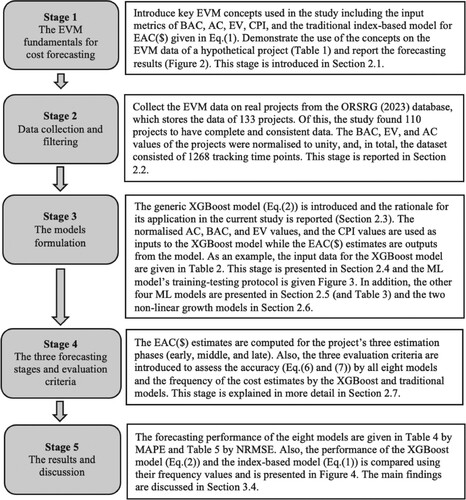
Our comprehensive methodology to develop the ML model for cost forecasting is presented in Figure 1. The approach follows five stages, which are explained in more detail in the following sections.

Figure 1. The research methodology.

This ML-based approach, presented in five stages and an alternative to the traditional EVM approach, is used to improve the final cost estimates in projects.

2.1. The EVM fundamentals for cost forecasting

EVM cost forecasting is based on three key metrics (PMI 2019): Planned value (PV) – the budgeted cost of the work scheduled; Earned value (EV) – the budgeted cost of the work performed; and Actual cost (AC) – the actual cost of the work performed. The total PV is the budget at completion (BAC), which refers to the total agreed budget of the project. Using these metrics, several performance measures could be derived.

The cost performance index (CPI = EV/AC) is used to assess how efficiently the project’s BAC is utilised at a certain time. Accurate cost predictions could be made using CPI if the project’s cost performance follows a similar pattern in the remaining life of the project (Anbari 2003). A CPI of 1.00 indicates that cost performance is on target; more than 1.00 indicates better than expected, and less than 1.00 indicates poor cost performance. The final cost of an ongoing project could be estimated using these metrics. Estimate at completion, EAC($) can be calculated as follows: (1) $\begin{array}{r}\mathrm{EAC}(\text{\$ }{)}_t=A{C}_t+\left(\mathrm{BAC}-E{V}_t\right)/\mathrm{CP}{I}_t\end{array}$(1) Where t is a tracking period measured in units of time.

For a given tracking period (e.g. month), this equation implies extrapolating the current AC realisation to the project’s end by adjusting the remaining BAC by the cumulative CPI. We demonstrate the calculation of EAC($) using the EVM data of a hypothetical project (Table 1). The project’s BAC is $700, and the planned duration is nine months. The reporting time (Actual time, AT) is the end of month 3, and at this time, EAC($) is calculated as $1,296. This value is much larger than the BAC as the project cost performance is much worse than expected at the reporting time (CPI <1.00). An S-curve depicted in Figure 2 shows this cost overrun.

Figure 2. A typical cost S-curve of a project.

A line graph, plotting the three curves of the planned, earned, and actual cost values in EVM, respectively, resembles a typical S-shape pattern.

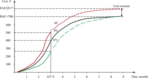
Table 1. The EVM data of a hypothetical project (the tracking period – month 3).

Time, months	PV, dollars	EV, dollars	AC, dollars	CPI	EAC($), dollars
1	50	40	80	0.50	1400
2	150	80	210	0.38	1838
3	400	270	500	0.54	1296
4	540	–	–	–	–
5	600	–	–	–	–
6	650	–	–	–	–
7	670	–	–	–	–
8	690	–	–	–	–
9	700	–	–	–	–

The cost estimate formulated in Equation (1) has been widely used as a standard in project cost forecasting (PMI 2019) and can be used when a few data points are available (Lipke et al. 2009). There are many more alternative formulations in the literature, i.e. the schedule performance index (SPI) or the combination of these two indexes, schedule and cost performance index (SCI) (Batselier and Vanhoucke 2015a; PMI 2019). However, in several comparison studies, the cost estimate formulated in Equation (1) has been the most accurate and/or stable (Batselier and Vanhoucke 2015a; De Marco, Rosso, and Narbaev 2016; PMI 2019). Therefore, we use this estimate as a benchmark in our study.

Although widely used approximation, as it is straightforward to calculate, the EAC($) calculation using Equation (1) has some drawbacks (İnan, Narbaev, and Hazir 2022; Kim and Reinschmidt 2011; Lipke et al. 2009; Warburton and Cioffi 2016). These drawbacks are due to the characteristics of the index-based models. First, it relies on only the past cost performance; (BAC-EV_t) is adjusted with CPI only, assuming that this index is the best available indicator of the future cost performance. Second, cost forecasting may be unreliable at the early stages of the projects because only a few data points are available for extrapolation. Lastly, using a conventional index-based model does not allow an understanding of the cost behaviour and the inherent patterns in data. In addition, all index-based models, including the one in Equation (1), assume linearity in cost growth. However, the cost growth pattern in projects is normally non-linear, usually an S-shaped pattern (Figure 2).

Considering the above limitations, we develop a new prediction model which could address the weaknesses of conventional EVM-based cost forecasting. Using ML, we aim to achieve much more accurate cost estimates than the ones computed with the above index-based model.

2.2. Data collection and filtering

We use the real project data shared by the Ghent University Operations Research and Scheduling research group (Batselier and Vanhoucke 2015b; ORSRG 2023). The database contains the scheduling, risk analysis, and project monitoring (i.e. EVM) data of 133 real-life projects. The projects are from the construction, information technology, and production industries.

First, we uploaded the EVM dataset of 133 projects into the Excel spreadsheets. The dataset had the following indicators and features for each project. The first indicator is BAC which represents the planned budget of a project. The minimum BAC of the projects is 1,210 dollars, the maximum is 62,385,597 dollars, and the average is 2,549,463 dollars. The second indicator is Cost at completion (CAC) which represents the actual cost of a project at completion. The EAC($) estimates were compared against this indicator for the accuracy analysis. Then, AC, EV, and CPI values were recorded. We normalised the EVM data because there are considerable differences in project budgets. To ensure data standardisation, we normalised the data for each project to unity. Therefore, each project’s BAC, CAC, AC, and EV data was normalised to unity, and, as a base, BAC was used.

Then, we cleaned the dataset. Among the 133, 23 projects do not have complete information on EV, AC, and/or consistent division into reporting periods (e.g. months). As a result, we kept 110 projects with data retrieved at 1268 tracking periods.

After the dataset cleaning, we divided each project’s tracking periods into three ranges representing the early, middle, and late stages. The range for the early stage is when the project is 1-29% work complete, for the middle stage – 30-69%, and for the late stage – 70-95% (Narbaev and De Marco 2014; Wauters and Vanhoucke 2017).

We note that for all eight models, we used the same dataset, indicators, and their features. Next, we explain the ML implementation.

2.3. The XGBoost model

Among the ML methods used in forecasting, we apply the XGBoost model. Based on the decision tree principles, its algorithm is large-scalable and highly adjustable to end-to-end ensemble tree-boosting systems for big data processing (Chen and Guestrin 2016). It belongs to the family of supervised ML models, which attempts to accurately predict a target variable by combining an ensemble of estimates from a set of simpler and weaker models. It is an ML algorithm that is based on the boosting model developed by Friedman (2001). According to Jabeur, Mefteh-Wali, and Viviani (2021), ‘normalization is used in the objective function to reduce model complexity, to prevent overfitting, and to make the learning process faster’. It belongs to the family of ensemble algorithms which applies an efficient realisation of decision trees, resulting in a combined model whose prediction capacity outperforms the ones by the individual algorithms when used alone Jabeur, Mefteh-Wali, and Viviani (2021). Overall, this ML model performs well because of its robust handling of various data types, relationships, and hyper-parameters that one can fine-tune. We refer to the paper of Chen and Guestrin (2016) for the details of the XGBoost model.

The formal additive function of the XGBoost is defined as per Equation (2) (Chen and Guestrin 2016). (2) $\begin{array}{r}L\left(\mathrm{\Phi }\right)=\sum _{i=0}^{n}l\left({\hat{y}}_i,y_i\right)+\sum _{k=1}^K\mathrm{\Omega }\left(f_k\right)\end{array}$(2) where i is the given case, n is the number of cases, and $\mathrm{\Omega }\left(f\right)=\mathrm{\gamma T}+\frac{1}{2}\lambda \parallel \omega {\parallel }^2$.

The L component is a differentiable convex loss function that measures the difference between the forecasted ${\hat{y}}_i$ and the actual $y_i$. The Ω term is a regularisation term to avoid overfitting, and it smooths the learned weights $\omega$. In this regard, this term penalises the complexity of the regression-based tree functions. T corresponds to the number of leaves in the tree. The γ and λ terms are the regularisation degrees. Each $f_k$ corresponds to an independent tree structure and leaf weights $\omega$.

In recent years, the XGBoost model has become popular in applied ML for classification and regression purposes due to its performance and fastness (Jabeur, Mefteh-Wali, and Viviani 2021; Uddin, Ong, and Lu 2022). For example, the comparative study with 20 ML models for budget forecasting in project management found the XGBoost model to be the most accurate with the lowest estimate error (Elmousalami 2021). The study empirically verified its high scalability, handling of missing values, high accuracy, and low computational cost as the model’s strengths compared to other ML models.

2.4. The XGBoost model inputs and training-testing protocol

We used the Python coding language (“Python 3.0 Release” 2023) to code the XGBoost algorithm. To run the model and make EAC($) predictions, we used the Jupyter Notebook tool, including the Python language. This is an open-source and cloud-based tool (“Project Jupyter” 2023). On Jupyter, codes and data are accessible from anywhere; all needed is to know a computer’s server number and password.

The EVM data stored in the Excel spreadsheets were used as inputs for this ML model. In particular, the input to embed into the XGBoost model in Python is the model presented in Equation (1) with four corresponding features: the AC, BAC, EV, and CPI values. Other than CPI values, the three input features were normalised to unity. For example, Table 2 presents the EVM data and the four input features (BAC norm, EV norm, AC norm, and CPI) for a project’s early stage. These four EVM metrics were taken as the x independent variables in the XGBoost model, while the EAC($) values as the y response variable, the output from the model. The index-based cost forecasting model in Equation (1) was integrated into the ML code for learning purposes.

Table 2. The EVM data and inputs to the XGBoost model (the early-stage estimation).

Project ID	BAC, dollars	EV, dollars	AC, dollars	BAC norm	EV norm	AC norm	CPI	CAC norm
1	180485	13527	13527	1.00	0.07	0.07	1.00	1.00
2	180759	22455	23427	1.00	0.12	0.13	0.96	1.06
3	484398	48729	49235	1.00	0.10	0.10	0.99	1.02
4	3027133	253805	283419	1.00	0.08	0.09	0.90	1.02
5	21369836	263753	269856	1.00	0.01	0.01	0.98	1.22
…	…	…	…	…	…	…	…	…
106	4318950	470150	386654	1.00	0.11	0.09	1.22	0.98
107	1456000	418322	424560	1.00	0.29	0.29	0.98	1.01
108	1512000	118037	119087	1.00	0.08	0.08	0.99	1.01
109	107500	1400	4000	1.00	0.01	0.04	0.35	1.09
110	114700	5700	6050	1.00	0.05	0.05	0.94	1.12

Note: Project ID refers to the projects’ order in the dataset (from 1 to 110) and not to the number of projects. The number of projects used in the early-stage estimation is 99.

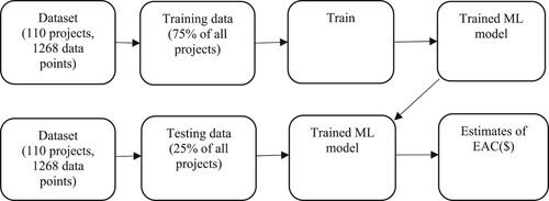
To perform the EAC($) predictions, we employed the training-testing protocol presented in Figure 3. In ML, datasets were divided into two subsets. The first is the training set, which is the dataset fed into an ML model to learn patterns. For the current study, the XGBoost model was trained using 75% of the total dataset. The remaining 25% was used for testing and to see if the model learns effectively from the patterns in the training dataset. ML algorithm randomly divides the total number of projects into 75% for the training set and 25% for the testing set. Then, the model performed 100 random trials for the testing to generate 100 corresponding EAC($) values as outputs. This random effect achieved from the 100 trials ensures consistency. Therefore, each run’s Mean absolute percentage error (MAPE) refers to the average of the 100 trials. In addition, the testing on 100 random trials was repeated 5 times to represent 5 independent runs, that is, 5 independent selections of the 25% of the projects for the testing set. In total, the final MAPE results in the study were based on 500 random estimates.

Figure 3. The training-testing protocol of the ML algorithm.

A flowchart, representing training and testing processes separately, depicts the process of implementing the ML algorithm to the EVM project data to estimate the final project cost.

2.5. Comparison with the other ML models

We compared our proposed XGBoost model with the other ML algorithms and non-linear regression models. The Random forest (RF), Support vector regression (SVR), LightGBM, and CatBoost models were selected among the ML methods.

As with the XGBoost algorithm, we used the Python tool library to derive the algorithms for these models and the Jupyter Notebook tool to calculate the EAC($) values. All five ML models had the same four inputs from the EVM dataset and the same training-testing framework presented in Figure 3. The details of these inputs and protocols are presented in Section 2.4. Next, we provide a pertinent description of the four models. Table 3 provides an overview of their parameter settings and explanation.

Table 3. The ML models, their parameter settings and explanation.

Model	Parameter settings	Parameter explanation
XGBoost	reg_alpha = 7, 6, and 5 (for the early, middle, and late forecasting stages, respectively)	Penalises the complexity of the function leading to finding features that do not improve accuracy.
Random forest	max_depth = 3; n_estimators = 90	Max_depth determines the maximum depth of each tree, allowing each tree in the data to increase until every leaf is considered. The n_estimators defines the number of trees in the forest.
Support vector regression	kernel = rbf by GridSearchCV, C = 10, gamma = auto	The kernel parameter manages complex (non-linear) relationships between the input and output cost variables. The C parameter manages the trade-off between the regularisation term and the training accuracy. The gamma parameter defines the curvature of the kernel function with larger values capturing better the training data, and the lower values resulting in smoother reflecting to testing data.
LightGBM	max_depth = 3, num_leaves = 10	Max_depth determines the maximum depth of each tree, allowing each tree in the data to increase until every leaf is considered. The num_leaves manages the maximum number of leaves (complexity) in one tree.
CatBoost	depth = 4, iterations = 100, learning_rate = 0,07	Max_depth determines the maximum depth of each tree, allowing each tree in the data to increase until every leaf is considered. The learning-rate parameter helps to optimise the training process from the input data given the number of iterations decrease.

RF is one of the bagging ensemble learning models that can produce accurate performance without overfitting issues (Breiman 2001). RF algorithm draws bootstrap samples to develop a forest of trees based on random subsets of features. An extremely randomised tree algorithm merges the randomisation of random subspace to a random cut-point selection during the splitting tree node process. Extremely randomised trees mainly control attribute randomisation and smoothing parameters (Geurts, Ernst, and Wehenkel 2006). Unfortunately, RF does not have such parameters as XGBoost does to impose penalties in forecasting. For this model, we used parameters ‘max_depth’ = 3; 4; 5 (respectively, for the three project estimation stages) and ‘n_estimators’ = 90 (Random Forest algorithm for Python. sklearn.ensemble. RandomForestRegressor) to improve the forecasting. The hyperparameter ‘max_depth’ was used to identify the depth of each decision tree, while ‘n_estimators’ handled how many generalised trees there should be in the forest. Different values for both parameters were tested, but only the above values showed improvements by a small margin compared to the estimation without the parameter settings. Different values were used for depth because the number of projects from the dataset in each forecasting stage was different.

SVR is a type of machine learning algorithm used for regression analysis. SVR aims to find a function that approximates the relationship between the input variables and a continuous target variable while minimising the prediction error (Smola and Schölkopf 2004). This algorithm has three parameters: kernel, gamma, and C (Scikit learn developers 2023). The kernel parameter is always used by default as RBF (the radial base function), which is evaluated only from the distance between points. In fact, this parameter is considered the most effective for regression and smoothly separating the input data without knowing data types. The gamma parameter is used as ‘auto,’ and calculated as ‘1/n_features’. It determines how many columns or functions the dataset has. Since, in our study, each forecasting stage has a different number of projects, the best decision was to put the value as ‘auto.’ The C parameter is a hypermeter that controls the prediction errors. A low value refers to low error. This parameter value ranges between 0.01–100. After multiple trials, the best value for the forecasting was chosen as 10.

LightGBM is a gradient-boosting ensemble model that is used by the Train Using AutoML tool and is based on decision trees. As with other decision tree-based methods, LightGBM can be used for both classification and regression. LightGBM is optimised for high performance with distributed systems. LightGBM uses a histogram-based method in which data is bucketed into bins using a distribution histogram (Ke et al. 2023). Instead of each data point, the bins are used to iterate, calculate the gain, and split the data. This method can be optimised for a sparse dataset as well. Another characteristic of LightGBM is exclusive feature bundling, in which the algorithm combines exclusive features to reduce dimensionality, making it faster and more efficient. Since this method uses the growth of a tree over, it is more prone to retraining and overfitting. Therefore, limiting the number of leaves in the tree was very important for which the hyperparameter ‘num_leaves’ = 10 was responsible. Together with this, it was necessary to reduce the size of the depth of the trees, ‘max_depth’ = 3 (Microsoft Corporation 2023).

CatBoost is another algorithm that uses binary decision trees as base predictors. A model built by a recursive partition of the feature space into several disjoint regions (tree nodes) according to the values of some splitting attributes a. Attributes are usually binary variables that identify that some feature x^k exceeds some threshold t, that is, a = 1{x^k> t}, where x^k is either numerical or binary feature; in the latter case t = 0.5. Each final region (leaf of the tree) is assigned to a value, which estimates the response y in the region for the regression task (Prokhorenkova et al. 2023). The following parameters were considered for CatBoost (Yandex 2023). The number of iterations was considered since it was responsible for building the maximum number of trees. This algorithm is considered important for configuration, can default to 1000 trees, and apply as many functions as possible. Given that our EVM dataset had 110 projects with a certain number of tracking periods, CatBoost would not work if corrected. The parameter ‘depth’ (the same as ‘max_depth’ in LightGBM) shows the depth of the tree. Then, in order to speed up the learning, we increased the value of ‘learning_rate’ (given the number of ‘iterations’ was reduced) as it directly depends on and is determined by ‘iterations’. In summary, after numerous experiments and controls of the value ‘learning_rate,’ the best result for its value was found to be 0.07 for all three forecasting stages.

2.6. Comparison with the non-linear regression models

We recall that the cost growth curve in projects resembles a non-linear S-shape (Bhaumik 2016; Pellerin and Perrier 2018) which typical characteristics are given in Figure 2. To this end, the non-linear regression models have been recognised as alternatives to the linear index-based models as they can capture the inherent non-linear relationship between project time and cost (Ballesteros-Pérez, Elamrousy, and González-Cruz 2019). Among the non-linear models, the so-called growth models use the nonlinear regression and are found to be reliable in cost curve fitting (Willems and Vanhoucke 2015).

Among the first works which analysed the predictive power of the cost forecasting methods using the growth models was the study by Trahan (2009). In this study, the researcher empirically tested the Gompertz growth model (GGM) using the EVM data of the U. S. Air Force acquisition contracts from 1960 to 2007. Later, Narbaev and De Marco (2014) conducted a study where they refined this GGM model and suggested the Logistic growth model (LGM) for EAC($) calculations.

For our comparative analysis with the ML models in this study, we adopt the cost forecasting approach of Narbaev and De Marco (2014) and apply GGM and LGM. Their approach is based on non-linear regression modelling and integrates the EVM and growth model concepts. It is defined as per Equation (3): (3) $\begin{array}{rl}\mathrm{EAC}(\mathrm{\$}{)}_t& =A{C}_t+\left[\mathrm{GrowthModel}\right(C{F}_t)\\ & -\mathrm{GrowthMode}{l}_t]\ast \mathrm{BAC}\end{array}$(3) where GrowthModel represents the function of a selected growth model, Completion Factor represents the index of project duration completion normalised to unity (which is equal to the inverse of Schedule Performance Index), and t represents the current tracking period.

If GrowthModel in Equation (3) is GGM, then it is defined as per Equation (4): (4) $\begin{array}{r}\mathrm{GGM}=\alpha \ast \text{exp}\left[-\exp \left(\text{β}-\mathrm{\gamma t}\right)\right]\end{array}$(4)

If GrowthModel in Equation (3) is LGM, then it is defined as per Equation (5): (5) $\begin{array}{r}\mathrm{LGM}=\alpha /\left[1+\exp \left(\text{β}-\mathrm{\gamma t}\right)\right]\end{array}$(5) where the $\alpha$ is the asymptote of the final cost as time t tends to infinity, $\text{β}$ is the $y$-intercept parameter representing the initial value of the project cost, and the $\gamma$ is the scale parameter that accounts for the growth rate of project cost, defining the curve shape.

Narbaev and De Marco (2014) compared the two non-linear regression models with the traditional EVM models and found their superiority in providing more accurate cost estimates. Later, Simion and Marin (2018) and Huynh et al. (2020) achieved similar results. Overall, the GGM and LGM have been found to generate more accurate estimates than the traditional index-based models, and our task in this study is to verify if they are also more accurate than the ML models.

For applying the two non-linear models, we followed the 3-stepped forecasting procedure given by Narbaev and De Marco (2014) (namely, Figure 3 in this reference). Minitab software package was used with its library storing the formulas for the GGM and LGM models. Unlike the computations for the cost estimates using the ML models (performed in Phyton automatically), the computations using the two non-linear models were conducted manually. We loaded each project data into Minitab and then exported the generated three parameters’ values of the GGM and LGM models (Equations (4) and (5), respectively) into the Excel spreadsheets for a further cost estimate with Equation (3).

2.7. The forecasting stages and the evaluation criteria

In the EVM literature, the cost forecasting for an ongoing project can be performed at each tracking period or a given project stage. In EVM forecasting, project life is divided into three stages: early, middle, and late. The literature defines the ranges for each stage (Narbaev and De Marco 2014; Wauters and Vanhoucke 2017). The range for the early stage is when the project is 1-29% work complete, for the middle stage – 30-69%, and for the late stage – 70-95%. Using ranges is somewhat more plausible than the work percent complete since the number of tracking periods (e.g. a several-month project versus a few-dozens-months project) and the EVM values (e.g. the budget size) differ from project to project. From the practical point of view, the EAC($) computations in the early and middle stages are more important than the ones in the late stage. This is because the cost control actions implemented upon an effective project forecasting system are essential at the beginning or middle of the project life. Timely corrective actions at these stages to the project budget and scope return a higher value than in the late stage when a project is close to completion. In practice, the value of the cost forecasting for an ongoing project diminishes as the project tends to its completion.

Next, we use the following three criteria in the current work to assess the quality of the index-based, ML-based, and non-linear regression cost forecasting models. They are used to measure the accuracy and frequency of the cost estimates.

The MAPE measures the estimate’s accuracy (Bates and Watts 1988). The average of the absolute values of the differences between the predicted EAC($) and the actual CAC of a project is calculated for a set of projects and each (early, middle, and late) project stage as per Equation (6): (6) $\begin{array}{r}\mathrm{MAPE},\text{\%}=\frac{1}{n}\sum _{i=1}^n\frac{|\mathrm{EAC}{\left(\text{\$ }\right)}_i-\mathrm{CA}{C}_i|}{\mathrm{CA}{C}_i},\text{\%}\end{array}$(6) where i is the given project, and n is the number of projects.

The result of MAPE can be classified as excellent if it is below 10.00, good between 10.00 and 20.00, and acceptable between 20.00 and 50.00 (Loop et al. 2010). However, we opt for a more conservative classification of MAPE results: the high accuracy level (MAPE is below 10.00), the moderate accuracy level (MAPE is below 20.00 but more than 10.00), and unacceptable level (MAPE is more than 20.00) (Peurifoy and Oberlender 2002).

The second criterion is the Root Mean Square Error (RMSE) which assesses the average difference between the cost estimates and the actual values. This metric suggests the narrowness of a forecast error, and its smaller value implies that the estimates by a given model are closer to its actual values and therefore generate more precise predictions (Seber and Wild 1989). However, this measure is based on absolute values. In our study the EVM data (budget inputs of the projects) is normalised to BAC to consider the differences in project budgets (scale-independence). Therefore, the normalised version of this measure (NRMSE) is used to analyse the deviations of the residuals of the estimates, defined as per Equation (7). (7) $\begin{array}{r}\mathrm{NRMSE}=\frac{\sqrt{\frac{1}{n}\sum _{i=1}^n{\left(\mathrm{EAC}{\left(\mathrm{\$}\right)}_i-\mathrm{CA}{C}_i\right)}^2}}{\mathrm{Average}\mathrm{of}\mathrm{BACs}}\end{array}$(7) where i is the given project, and n is the number of projects.

The third criterion used in the study is the number of projects at which the best-performing model gives more accurate results than the index-based benchmark model. It will be presented using a histogram.

3. Results and discussion

3.1. Descriptive statistics and convergence considerations

Before we report the forecasting results, we present the following statistics of the 110 projects and considerations regarding the non-linear regression curve fitting. For the early-stage estimation, the data of 99 projects were used; for the middle-stage estimation – of 107 projects; and for the late-stage estimation – of all 110 projects. Mean cost deviation (MCD), which represents the average of deviations of CAC (the actual cost) from BAC (the budgeted cost) for all projects, was 3.92% in the early stage, 3.70% in the middle stage, and 1.87% in the late stage. Positive values of MCD in all three stages imply that, on average, the projects in our dataset were delivered with budget overruns. MCD is calculated as per Eq.(8). (8) $\begin{array}{r}\mathrm{MCD},\text{\%}=\frac{1}{n}\sum _{i=1}^n\frac{|\mathrm{CA}{C}_i-\mathrm{BA}{C}_i|}{\mathrm{BA}{C}_i},\text{\%}\end{array}$(8) where i is the given project, and n is the number of projects.

Regarding the application of the non-linear GGM and LGM, first, it was essential to estimate their three parameters (the $\alpha ,\text{β},\text{and }\gamma$) given in Equations (4) and (5). Second, after the Minitab determines the values of the parameters through the non-linear regression curve fitting, the defined values are loaded into the non-linear EAC($) formula in Equation (3). However, the critical task in non-linear regression curve fitting is to define the values of the model’s parameters (Bates and Watts 1988). Minitab performs this task using the approximation approach (the Gauss–Newton approximation was used) for the two non-linear models. For this reason, we regarded the GGM and LGM as statistically valid if this approximation converges to estimate the values for their parameters. If this approximation fails to converge, then the curve fitting process does not return the values for the three parameters of the GGM and LGM models for a given project data from the dataset. The cause of this failure, as noted by Narbaev and De Marco (2014) is multicollinearity in the curve fitting, which occurs in multiple regressions when two or more predictors are highly correlated and leads to erratic changes in the parameter estimates. Subsequently, for such projects, it was impossible to apply Equation (3) for the EAC($) forecasting, and they were disregarded from the further comparative analysis with the index-based and ML models. It is one of the significant drawbacks of the curve fitting using the non-linear regression, as the number of projects was not the same for all comparing models in the study.

In the current study, for the early-stage estimation of 99 total projects in the dataset, 88 cases were valid for cost forecasting using GGM and 78 using LGM (disregarding 11 and 21 projects, respectively). For the middle-stage estimation, among 107 cases, 95 were valid for GGM and 79 for LGM (removing 12 and 28 projects, respectively). For the late-stage estimation, among 110 projects in the dataset, 98 were valid for the estimation with GGM and 85 with LGM (disregarding 12 and 25 projects, respectively).

3.2. The EAC($) accuracy results

After validating the XGBoost model (Equation 2), we computed EAC($) estimates for three stages of the projects. Then, we computed EAC($) estimates using the index-based model Equation (1), the other ML models (RF, SVR, LightGBM, and CatBoost), and the non-linear growth models (GGM and LGM). We followed the training-testing framework for all five ML applications presented in Figure 3. To validate the non-linear GGM and LGM models, we followed the 3-stepped forecasting approach of Narbaev and De Marco (2014) using Minitab. Lastly, we compared the cost estimates of the eight models using their MAPE and RMSE values. Therefore, we aim to define which of the models is best for forecasting EAC($)s at the early, middle, and late stages of the project execution. The summary of the MAPE results for the eight models is presented in Table 4, and the NRMSE results are in Table 5. For each forecasting stage with the five ML models, we performed 5 random runs as described in Section 2.4.

Table 4. The accuracy results of the forecasting models, MAPE%.

	Project stages
Model	Early	Middle	Late
MCD	3.92	3.70	1.87
Index-based model	17.43	15.35	14.35
XGBoost	Range: 6.53-9.70	Range: 6.42-8.57	Range: 6.22-8.28
Run 1	7.85	8.57	7.40
2	9.70	6.81	7.97
3	6.53	7.16	8.28
4	8.37	6.42	6.22
5	9.54	8.43	7.74
Random forest	Range: 13.44-14.51	Range: 12.51-13.89	Range: 11.84-12.92
Run 1	14.11	13.10	12.08
2	13.73	12.99	12.28
3	13.44	12.51	12.92
4	13.93	13.89	11.84
5	14.51	13.28	12.54
Support vector regression	Range: 17.92-18.82	Range: 14.14-16.86	Range: 11.34-15.52
Run 1	18.74	16.86	14.42
2	17.92	15.34	14.79
3	17.50	14.68	11.34
4	18.43	16.75	15.52
5	18.82	14.14	14.42
LightGBM	Range: 15.01-18.74	Range: 12.59-16.21	Range: 11.14-14.94
Run 1	15.93	15.81	11.14
2	16.18	12.59	12.98
3	15.01	14.59	13.93
4	17.42	13.19	14.94
5	18.74	16.21	14.19
CatBoost	Range: 13.97-14.92	Range: 11.56-12.54	Range: 11.48-12.52
Run 1	14.49	11.56	11.45
2	14.87	12.54	12.52
3	15.77	12.15	12.25
4	13.97	12.21	11.48
5	14.92	12.04	12.16
Non-linear GGM	25.41	21.14	6.64
Non-linear LGM	21.19	11.81	5.61

Note: for the early-stage estimation, of 99 projects in the dataset, GGM failed to obtain the convergence in 11 and LGM in 21 projects. For middle-stage estimation, of 107 projects, GGM failed to obtain the convergence in 12 and LGM in 28 projects. For the late-stage estimation, of 110 cases, GGM failed to obtain the convergence in 12 and LGM in 25 cases.

Table 5. The accuracy results of the forecasting models, NRMSE.

	Project stages
Model	Early	Middle	Late
Index-based	0.54	0.44	0.30
XGBoost	Range: 0.08-0.19	Range: 0.09-0.21	Range: 0.11-0.23
Run 1	0.15	0.09	0.19
2	0.08	0.16	0.11
3	0.19	0.12	0.16
4	0.13	0.14	0.23
5	0.18	0.21	0.20
Random forest	Range: 0.12-0.39	Range: 0.11-0.29	Range: 0.15-0.28
Run 1	0.19	0.24	0.15
2	0.23	0.17	0.28
3	0.12	0.11	0.26
4	0.39	0.12	0.18
5	0.27	0.29	0.23
Support vector regression	Range: 0.17-0.36	Range: 0.17-0.43	Range: 0.16-0.37
Run 1	0.28	0.17	0.23
2	0.36	0.13	0.16
3	0.31	0.43	0.29
4	0.35	0.28	0.22
5	0.17	0.22	0.37
LightGBM	Range: 0.18-0.29	Range: 0.13-0.23	Range: 0.14-0.21
Run 1	0.18	0.23	0.14
2	0.19	0.22	0.17
3	0.22	0.13	0.21
4	0.29	0.21	0.18
5	0.23	0.17	0.20
CatBoost	Range: 0.17-0.41	Range: 0.16-0.39	Range: 0.10-0.35
Run 1	0.37	0.16	0.30
2	0.20	0.23	0.10
3	0.24	0.27	0.21
4	0.17	0.39	0.35
5	0.41	0.18	0.17
Non-linear GGM	0.27	0.18	0.11
Non-linear LGM	0.18	0.24	0.13

Note: for the early-stage estimation, of 99 projects in the dataset, GGM failed to obtain the convergence in 11 and LGM in 21 projects. For middle-stage estimation, of 107 projects, GGM failed to obtain the convergence in 12 and LGM in 28 projects. For the late-stage estimation, of 110 cases, GGM failed to obtain the convergence in 12 and LGM in 25 cases.

For the early-stage estimates, the results show that the range of MAPE with the XGBoost model is 6.53-9.70. The MAPE value computed by the index-based model is comparatively high, 17.43. The errors of the other four ML models are like the ones by the index-based model ranging between 13.00 and 18.00. The non-linear GGM and LGM forecasting errors are even higher, at 15.41 and 21.19. Moreover, we note that, due to failing to obtain the convergence in estimating the values for their parameters by these models, 11 and 21 projects, respectively, were disregarded from the analysis.

The XGBoost model provides more accurate EAC($) also in the middle and late stages; the MAPE range of 6.42-8.57 against 15.35 by the benchmark index-based model in the middle stage, and the range of 6.22-8.28 against 14.35 in the late stage. The estimates by the other four ML models are less accurate than the ones by the XGBoost model and compared to the estimates by the index-based model, with the MAPE ranges between 11.00 and 17.00 in both forecasting stages. We note more accurate estimates by the two non-linear models in the late stage (GGM’s MAPE = 6.64 and LGM's MAPE = 5.61). However, they should be carefully compared due to the convergence issue and disregarded cases explained above for these two models.

The results of the NRMSE follow a similar tendency. This metric implies the narrowness of the estimate's error, i.e. the deviation of the residuals. The estimates by the index-based model report higher values of NRMSE, which are 0.54, 0.44, and 0.30 for the three estimation stages, respectively. Among the five ML models, the XGBoost generated better NRMSE values. The non-linear GGM and LGM values suggest better estimates in the late stage compared to all other models. However, as noted above, the forecasting by these models encountered the convergence issue in 12 and 25 projects, respectively, out of 110. Consequently, comparing their estimates with the ones by the index-based and ML models, which report the estimates of all 110 projects, should not be appropriate.

To summarise, in all the forecasting stages, the MAPE range by the XGBoost model is from 6.22–9.70, while the one by the index-based model is from 14.35–17.43, and the estimates by the other ML models have the MAPE range between 11.00 and 18.00, approximately. The differences in error are significant. The MAPE of below 10.00 in the project cost forecasting literature is regarded as excellent (the high accuracy level), while the MAPE below 20.00 is good (the moderate accuracy level). Overall, the XGBoost model outperforms the traditional index-based model, the four ML (RF, SVR, LightGBM, and CatBoost), and non-linear models (GGM and LGM) in all three stages of the project execution. This implies the proposed model’s overall performance for high accuracy in project cost forecasting.

3.3. The EAC($) frequency results

To compare the frequency results with the index-based benchmark model, we selected the best-performing XGBoost model. Figure 4 presents the results of the frequency analysis. For the XGBoost and the index-based models, it compares their cost estimates and reports the number of projects (frequency) when one model performs more accurately and is more stable during the work than the other. The number of projects in Figure 4 is 25, 27, and 28 for the early-stage, middle-stage, and late-stage estimation, respectively. These numbers correspond to 25% of the total projects in the dataset, used as a threshold to randomly select the projects for the testing phase of the XGBoost model.

Figure 4. The number of more accurate cases (frequency of projects) by the XGBoost and index-based benchmark models.

A chart, contrasting the estimates’ frequency by the index-based model and the XGBoost model, shows that the performance of XGBoost is significantly better in forecasting the final project cost.

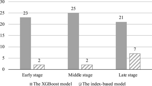
For the early-stage estimation, the index-based model’s MAPE is 17.43 (Table 4), and this value was taken as a threshold to compare the estimates’ errors by the XGBoost model in the early stage. In 23 of the 25 cases, our proposed model performed more accurately than the traditional index-based model (i.e. its errors were lower than MAPE = 17.43). Based on the results, the proposed model provided more accurate EAC($) estimates in 92.00% of the instances, which is substantially superior to the index-based model, which outperformed in only 8.00% of the cases. In the middle stage, on average, the XGBoost algorithm performed more accurately in 92.59% of the cases. Lastly, close to the end of the project execution, the proposed model’s cost estimates were more accurate than the index-based model’s in 75.00% of the projects randomly taken in the testing phase.

3.4. Main findings and discussion

We evaluate the performance of the algorithms based on the overall accuracy level, the accuracy level at early stages of project life (timeliness), and the project-based prediction performance. We also explore and discuss the XGBoost model’s characteristics compared to the other models.

Based on the overall accuracy of the EAC($) estimates, the XGBoost algorithm provides much more accurate forecasts than the index-based benchmark, the other four ML, and the two non-linear models. The difference between the accuracy levels is considerable at each project stage (Table 4). The conventional EVM-based technique (represented by the benchmark model in Equation (1)) in cost forecasting is prone to high errors. The RF, SVR, LightGBM, and CatBoost generated comparatively high errors in the forecasts in each three estimation stages. The non-linear GGM and LGM models also produced less accurate estimates in the early and middle stages of the projects. However, they generated more accurate EAC($)s in the late stage. However, for some project data, these regression models failed to converge in estimating their parameters’ values (the $\alpha$ asymptote, $\text{β}$ $y$-intercept, and $\gamma$ scale in Equations (4) and (5), respectively). In about 10.90-11.21% of the projects used, the GGM failed to estimate the parameters’ values and, consequently, to calculate the cost estimates for comparison. The LGM model failed to utilise the data of about 21.21-28.28% of projects for the same reason. In this study, we corroborated the convergence issue of the non-linear regression in curve fitting with the previous studies (e.g. Narbaev and De Marco (2014)). Consequently, we did not compare the estimates by the two models with the ones given by the index-based and the ML models in the study. We next elaborate on the overall performance of the XGBoost model concerning the other ML algorithms and the index-based model, in particular.

First, this is due to the limitation of the conventional index-based model, which assumes that the past cost performance (from completed tracking periods) in an ongoing project is the sole information used for the EAC($) estimates (see Section 2.1). In particular, the cost estimate has two summands: AC and the value of the remaining work (BAC-EVt). While AC cannot be modified as it is incurred, the remaining work in a project is adjusted by CPI, which is assumed to be the only available indicator. This is a limitation of the index-based models, which implies that the project work will continue as per its past performance till it finishes. However, the project environment is uncertain, and due to such changing circumstances, project managers often revise their project budgets. The second drawback of the traditional models is their poor ability to understand the cost behaviour and capture the inherent patterns in past performance. This is associated with the assumption of linearity in cost spending in projects.

The ML models address these two drawbacks in the current study. Unlike the benchmark model, the ML models (with the XGBoost algorithm as the best performer) learn from the given EVM data in the training phase (see Figure 3). Then, they apply the acquired knowledge on the past cost performance of the EAC($) forecasting in the testing phase (see Figure 3). The learning process utilises the dataset’s four variables; AC, BAC, EV, and CPI. Also, the learning is based on the non-linear regression features embedded into the XGBoost algorithm modelling (Chen and Guestrin 2016; Jabeur, Mefteh-Wali, and Viviani 2021).

The second finding is on the accuracy of estimates made at the initial stages of the project execution. Defined as timeliness in cost forecasting, it is the feature of a model to provide more accurate estimates as earlier as possible. This is a practical concern in project control since project managers are often attentive to the cost forecasting approaches, allowing for early warning signals for more effective cost control. Also, the accuracy of the forecasts in the early and middle stages of the projects is more critical to project managers to take corrective actions on time. The decisions at the late stages might not be effective. The forecasting performance of the XGBoost model dominates the benchmark model and the other ML models at these critical early and middle stages (see Figure 4). In the early stage, the XGBoost model’s MAPE range is 6.53-9.70 compared to the index-based model’s MAPE of 17.43. The NRMSE range is 0.08-0.19 against 0.54. Moreover, in the middle stage, this is 6.22-8.28 compared to 15.35; the NRMSE range is 0.09-0.21 against 0.44. Based on the results, our study provides managers with a more reliable tool to support their project control decisions early in project life.

The findings also suggest that the proposed XGBoost model produced more accurate estimates in 92.00% of the projects tested in the early stage, 92.59% in the middle stage, and 75.00% in the late stages (see Figure 4). These frequencies are high. This proves the proposed model is reliable, providing more accurate EAC($) in most cases. It is also important as a cost forecasting method should produce more accurate or timely estimates and be consistent when repeatedly used in projects.

In Figure 4, the estimates for some projects are not improved by the XGBoost model, and we provide the following conjecture about this. The XGBoost model performs the initial prediction, after which residuals are calculated based on the predicted value and observed values. The decision tree is created with the residuals using the similarity score for the previous residuals. The similarity of the data in the leaf is calculated, as well as the gain in similarity in the subsequent split. The output value for each sheet is also calculated using the previous residuals. This process is repeated until the residuals no longer decrease. So, when such residuals no longer decrease, the model still tries to minimise the errors, but we use reg_alpha, which penalises the cases that increase the cost function. This means that it returns the estimates that still need to be improved.

Lastly, we found that the proposed XGBoost model, given its training-testing protocol in Figure 3, is effective overall for EAC($) estimation. This model handles high scalability of the cost data and processes largely deviated (noisy) cases within the given dataset. The scalability was addressed by normalising the three input variables (i.e. AC, BAC, EV) to unity. This was a crucial solution as the EVM data of projects had substantial differences in size. Also, the proposed model could fit the input data for more accurate estimates without high overfitting. Overfitting happens when a model precisely fits training data, hence, with a reduced ability to understand a new dataset (i.e. testing set). This problem is dealt with by the feature of the XGBoost model, which counts for the learning effect. Namely, the Ω regularisation term, given in Equation (2), allows learning from the training data and handles the overfitting issue. Overall, except for the above three main findings of the study, this was a methodological contribution of our study to bring the ML application into the traditional EVM cost forecasting area.

4. Conclusion

Cost forecasting is critical for effective project monitoring and control. Managers widely use simple EVM models to forecast the final cost of projects and control their budgets. However, we showed that such models are prone to the limitations inherent to their naive and linear nature, producing less accurate or/and unreliable cost estimates.

Based on ML applications, in the current study, we proposed the XGBoost algorithm-based model to forecast the total cost of projects. We used the real cost data of 110 projects to validate the model. We compared the forecasting performance of the XGBoost model to the one of the EVM index-based model (widely used in practice), the other ML models (RF, SVR, LightGBM, and CatBoost) and two non-linear models (GGM and LGM). The comparison criteria were the overall forecasting accuracy, timeliness, and project-based prediction performance (frequency). Regarding overall accuracy, the proposed model performed more accurately than the index-based and the other ML models, with considerable differences in the accuracy levels. Regarding timeliness, the XGBoost model also produced more accurate estimates earlier at the initial stages of the project execution, presenting early warning signals for more effective cost control. We also found that the model showed more accurate estimates in most projects tested, implying its overall reliability. It is crucial as a cost forecasting model should provide accurate and timely forecasts and be consistent when frequently used in practice.

Future studies can address the following limitation. The dataset included the projects undertaken mainly in Belgium and the construction industry. However, there is no public database that includes many more diverse projects. Therefore, the performance of the constructed algorithm can be tested using a more comprehensive database. Also, future research can include integrating cluster analysis and more ML approaches. For example, the projects can be clustered by type, and considering specific characteristics of each type (i.e. industry), a different ML approach could be proposed for each cluster. Second, in this study, we focused on cost forecasting. However, algorithms that specifically address time (schedule) forecasting could be developed. Another research direction can be understanding the causal relationship between the model outputs and the input variables and assessing the relative contribution of each such variable and feature. The Shapley additive explanations approach has been growing for such ML applications in recent years.

Disclosure statement

No potential conflict of interest was reported by the author(s).

Data availability statement

The authors confirm that the data supporting the findings of this study are available within the article and its supplementary materials.

Additional information

Funding

This work was supported by the Committee of Science of the Ministry of Science and Higher Education of the Republic of Kazakhstan under Grant AP09259049.

Notes on contributors

Timur Narbaev

Dr. Timur Narbaev is a professor at Business School of Kazakh-British Technical University (Almaty, Kazakhstan). His research interests are in project management and public-private partnerships. He has won several awards, including Thomson Reuters' Web of Science 2016 Science Leader Award, and was a finalist for IPMA 2014 Young Researcher Award. He is a member of the Project Management Institute, American Society of Civil Engineers, and a certified British Council trainer.

Öncü Hazir

Dr. Öncü Hazir is an associate professor at the Department of Supply Chain Management and Information Systems, Rennes School of Business (Rennes, France). He lectures on Supply chain management and Operations management courses. His recent research includes Project management, Inventory management, Machine scheduling, and Assembly line balancing. Email: [email protected]

Balzhan Khamitova

Balzhan Khamitova is a research fellow at Business School of Kazakh-British Technical University (Almaty, Kazakhstan). She holds an MS degree in project management and conducts research in Information technology applications in Project automation and control. She has served as a research intern in the project management world library, continually improving the library database https://pmworldlibrary.net/balzhan-khamitova/. Email: [email protected]

Sayazhan Talgat

Sayazhan Talgat is a research fellow at Business School of Kazakh-British Technical University (Almaty, Kazakhstan). Currently, she conducts research in Machine learning applications for more effective Project scheduling and control. Sayazhan participated in projects related to innovative start-ups and intelligent applications in financial analysis. Email: [email protected]

References

- Agrawal, Ajay, Joshua Gans, and Avi Goldfarb. 2020. “How to Win with Machine Learning.” Harvard Business Review. https://hbr.org/2020/09/how-to-win-with-machine-learning.
- Anbari, F. T. 2003. “Earned Value Project Management Method and Extensions.” Project Management Journal 34 (4): 12–23. https://doi.org/10.1109/EMR.2004.25113.
- Aramali, Vartenie, Hala Sanboskani, G. Edward, Jr. Gibson, Mounir El Asmar, and Namho Cho. 2022. “Forward-Looking State-of-the-Art Review on Earned Value Management Systems: The Disconnect Between Academia and Industry.” Journal of Management in Engineering 38 (3): 03122001. https://doi.org/10.1061/(ASCE)ME.1943-5479.0001019.
- Bakici, Tuba, Andre Nemeh, and Oncu Hazir. 2021. “Big Data Adoption in Project Management: Insights from French Organizations.” IEEE Transactions on Engineering Management. Institute of Electrical and Electronics Engineers Inc. https://doi.org/10.1109/TEM.2021.3091661.
- Ballesteros-Pérez, Pablo, Kamel Mohamed Elamrousy, and Ma Carmen González-Cruz. 2019. “Non-Linear Time-Cost Trade-off Models of Activity Crashing: Application to Construction Scheduling and Project Compression with Fast-Tracking.” Automation in Construction 97. https://doi.org/10.1016/j.autcon.2018.11.001.
- Bates, Douglas M., and Donald G. Watts. 1988. Nonlinear Regression Analysis and Its Applications. New York: John Wiley & Sons, Inc. https://doi.org/10.1002/9780470316757.
- Batselier, Jordy, and Mario Vanhoucke. 2015a. “Empirical Evaluation of Earned Value Management Forecasting Accuracy for Time and Cost.” Journal of Construction Engineering and Management 141 (11): 05015010. https://doi.org/10.1061/(ASCE)CO.1943-7862.0001008.
- Batselier, Jordy, and Mario Vanhoucke. 2015b. “Construction and Evaluation Framework for a Real-Life Project Database.” International Journal of Project Management 33 (3): 697–710. https://doi.org/10.1016/j.ijproman.2014.09.004.
- Bhaumik, Pradip K. 2016. “Developing and Using a New Family of Project S-Curves Using Early and Late Shape Parameters.” Journal of Construction Engineering and Management 142 (12), https://doi.org/10.1061/(asce)co.1943-7862.0001201.
- Bilal, Muhammad, and Lukumon O. Oyedele. 2020. “Big Data with Deep Learning for Benchmarking Profitability Performance in Project Tendering.” Expert Systems with Applications 147 (June): 113194. https://doi.org/10.1016/J.ESWA.2020.113194.
- Breiman, Leo. 2001. “Random Forests.” Machine Learning 45 (1): 5–32. https://doi.org/10.1023/A:1010933404324/METRICS.
- Chen, Zhi, Erik Demeulemeester, Sijun Bai, and Yuntao Guo. 2019. “A Bayesian Approach to Set the Tolerance Limits for a Statistical Project Control Method.” International Journal of Production Research 58 (10): 3150–3163. https://doi.org/10.1080/00207543.2019.1630766.
- Chen, Tianqi, and Carlos Guestrin. 2016. “XGBoost: A Scalable Tree Boosting System.” Proceedings of the 22nd ACM SIGKDD International Conference on Knowledge Discovery and Data Mining. New York, NY, USA: ACM. https://doi.org/10.1145/2939672.
- Cheng, Min-Yuan, Yu-Han Chang, and Dorcas Korir. 2019. “Novel Approach to Estimating Schedule to Completion in Construction Projects Using Sequence and Nonsequence Learning.” Journal of Construction Engineering and Management 145 (11): 04019072. https://doi.org/10.1061/(ASCE)CO.1943-7862.0001697.
- Choi, Tsan Ming, Stein W. Wallace, and Yulan Wang. 2018. “Big Data Analytics in Operations Management.” Production and Operations Management 27 (10): 1868–1883. https://doi.org/10.1111/POMS.12838.
- Dahmani, Sarra, Oussama Ben-Ammar, and Aïda Jebali. 2021. “Resilient Project Scheduling Using Artificial Intelligence: A Conceptual Framework.” IFIP Advances in Information and Communication Technology 630 IFIP, Springer Science and Business Media Deutschland GmbH: 311–320. https://doi.org/10.1007/978-3-030-85874-2_33.
- de Andrade, Paulo André, Annelies Martens, and Mario Vanhoucke. 2019. “Using Real Project Schedule Data to Compare Earned Schedule and Earned Duration Management Project Time Forecasting Capabilities.” Automation in Construction 99 (March): 68–78. https://doi.org/10.1016/j.autcon.2018.11.030.
- De Marco, Alberto, Marta Rosso, and Timur Narbaev. 2016. “Nonlinear Cost Estimates at Completion Adjusted with Risk Contingency.” Journal of Modern Project Management 4 (2): 24–33. https://doi.org/10.19255/JMPM01102.
- Elmousalami, Haytham H. 2021. “Comparison of Artificial Intelligence Techniques for Project Conceptual Cost Prediction: A Case Study and Comparative Analysis.” IEEE Transactions on Engineering Management 68 (1): 183–196. https://doi.org/10.1109/TEM.2020.2972078.
- Friedman, Jerome H. 2001. “Greedy Function Approximation: A Gradient Boosting Machine.” The Annals of Statistics 29 (5): 1189–1232. https://doi.org/10.1214/AOS/1013203451.
- Geurts, Pierre, Damien Ernst, and Louis Wehenkel. 2006. “Extremely Randomized Trees.” Machine Learning 63 (1): 3–42. https://doi.org/10.1007/S10994-006-6226-1/METRICS.
- Hall, Nicholas G. 2016. “Research and Teaching Opportunities in Project Management.” INFORMS Tutorials in Operations Research, October. INFORMS, 329–388. https://doi.org/10.1287/educ.2016.0146.
- Hu, Xuejun, Nanfang Cui, and Erik Demeulemeester. 2015. “Effective Expediting to Improve Project Due Date and Cost Performance Through Buffer Management.” International Journal of Production Research 53 (5): 1460–1471. https://doi.org/10.1080/00207543.2014.948972.
- Huynh, Quyet Thang, The Anh Le, Thanh Hung Nguyen, Nhat Hai Nguyen, and Duc Hieu Nguyen. 2020. “A Method for Improvement the Parameter Estimation of Non-Linear Regression in Growth Model to Predict Project Cost at Completion.” In Proceedings - 2020 RIVF International Conference on Computing and Communication Technologies, RIVF 2020. https://doi.org/10.1109/RIVF48685.2020.9140765.
- İnan, Tolga, Timur Narbaev, and Öncü Hazir. 2022. “A Machine Learning Study to Enhance Project Cost Forecasting.” IFAC-PapersOnLine 55 (10): 3286–3291. https://doi.org/10.1016/J.IFACOL.2022.10.127.
- Jabeur, Sami Ben, Salma Mefteh-Wali, and Jean Laurent Viviani. 2021. “Forecasting Gold Price with the XGBoost Algorithm and SHAP Interaction Values.” Annals of Operations Research, July, Springer, 1–21. https://doi.org/10.1007/S10479-021-04187-W/METRICS.
- Ke, Guolin, Qi Meng, Thomas Finley, Taifeng Wang, Wei Chen, Weidong Ma, Qiwei Ye, and Tie-Yan Liu. 2023. “LightGBM: A Highly Efficient Gradient Boosting Decision Tree.” Accessed June 25. https://dl.acm.org/doi/10.55553294996.3295074.
- Kim, Byung-Cheol. 2015. “Probabilistic Evaluation of Cost Performance Stability in Earned Value Management.” Journal of Management in Engineering 32 (1): 04015025. https://doi.org/10.1061/(ASCE)ME.1943-5479.0000383.
- Kim, Byung-Cheol, and Kenneth F. Reinschmidt. 2011. “Combination of Project Cost Forecasts in Earned Value Management.” Journal of Construction Engineering and Management 137 (11): 958–966. https://doi.org/10.1061/(asce)co.1943-7862.0000352.
- Kim, Eun Hong, William G. Wells, and Michael R. Duffey. 2003. “A Model for Effective Implementation of Earned Value Management Methodology.” International Journal of Project Management 21 (5): 375–382. https://doi.org/10.1016/S0263-7863(02)00049-2.
- Kose, Tekin, Tuba Bakici, and Oncu Hazir. 2022. “Completing Projects on Time and Budget: A Study on the Analysis of Project Monitoring Practices Using Real Data.” IEEE Transactions on Engineering Management, 1–12. https://doi.org/10.1109/TEM.2022.3227428.
- Li, Li, Yanfei Kang, Fotios Petropoulos, and Feng Li. 2022. “Feature-Based Intermittent Demand Forecast Combinations: Accuracy and Inventory Implications.” International Journal of Production Research. https://doi.org/10.1080/00207543.2022.2153941.
- Lipke, Walt, Ofer Zwikael, Kym Henderson, and Frank Anbari. 2009. “Prediction of Project Outcome. The Application of Statistical Methods to Earned Value Management and Earned Schedule Performance Indexes.” International Journal of Project Management 27 (4): 400–407. https://doi.org/10.1016/j.ijproman.2008.02.009.
- Loop, Benjamin P., Scott D. Sudhoff, Stanislaw H. Zak, and Edwin L. Zivi. 2010. “Estimating Regions of Asymptotic Stability of Power Electronics Systems Using Genetic Algorithms.” IEEE Transactions on Control Systems Technology 18 (5): 1011–1022. https://doi.org/10.1109/TCST.2009.2031325.
- Mahmoudi, Amin, Morteza Bagherpour, and Saad Ahmed Javed. 2021. “Grey Earned Value Management: Theory and Applications.” IEEE Transactions on Engineering Management 68 (6): 1703–1721. https://doi.org/10.1109/TEM.2019.2920904.
- Martens, Annelies, and Mario Vanhoucke. 2018. “An Empirical Validation of the Performance of Project Control Tolerance Limits.” Automation in Construction 89 (May): 71–85. https://doi.org/10.1016/J.AUTCON.2018.01.002.
- Merhi, Mohammad I., and Antoine Harfouche. 2023. “Enablers of Artificial Intelligence Adoption and Implementation in Production Systems.” International Journal of Production Research. https://doi.org/10.1080/00207543.2023.2167014.
- Microsoft Corporation. 2023. “LightGBM Algorithm for Python.” https://xgboost.readthedocs.io/en/latest/parameter.html.
- Munir, Maria. 2019. “How Artificial Intelligence Can Help Project Managers.” Global Journal of Management and Business Research 19 (A4): 29–35. https://journalofbusiness.org/index.php/GJMBR/article/view/2728/2-How-Artificial-Intelligence_html.
- Narbaev, Timur, and Alberto De Marco. 2014. “Combination of Growth Model and Earned Schedule to Forecast Project Cost at Completion.” Journal of Construction Engineering and Management 140 (1), https://doi.org/10.1061/(ASCE)CO.1943-7862.0000783.
- Narbaev, Timur, and Alberto De Marco. 2017. “Earned Value and Cost Contingency Management: A Framework Model for Risk Adjusted Cost Forecasting.” Journal of Modern Project Management 4 (3): 12–19. https://doi.org/10.19225/JMPM01202.
- Ong, Stephen, and Shahadat Uddin. 2020. “Data Science and Artificial Intelligence in Project Management: The Past, Present and Future.” Journal of Modern Project Management 7 (4): 1–8. https://journalmodernpm.com/manuscript/index.php/jmpm/article/view/JMPM02202.
- ORSRG. 2023. “Real Project Data.” Operations Research & Scheduling Research Group. Accessed January 16. https://www.projectmanagement.ugent.be/research/data/realdata.
- Owolabi, Hakeem A., Muhammad Bilal, Lukumon O. Oyedele, Hafiz A. Alaka, Saheed O. Ajayi, and Olugbenga O. Akinade. 2020. “Predicting Completion Risk in PPP Projects Using Big Data Analytics.” IEEE Transactions on Engineering Management 67 (2): 430–453. https://doi.org/10.1109/TEM.2018.2876321.
- Pellerin, Robert, and Nathalie Perrier. 2018. “A Review of Methods, Techniques and Tools for Project Planning and Control.” International Journal of Production Research 57 (7): 2160–2178. https://doi.org/10.1080/00207543.2018.1524168.
- Peurifoy, Rober L., and Garold D. Oberlender. 2002. Estimating Construction Costs. Boston: McGraw-Hill. https://www.abebooks.com/Estimating-Construction-Costs-Mcgraw-Hill-Series-Engineering/30859894889/bd.
- PMI. 2019. The Standard for Earned Value Management. https://www.pmi.org/pmbok-guide-standards/foundational/earned-value-management.
- “Project Jupyter”. 2023. Accessed January 16. https://jupyter.org/.
- Prokhorenkova, Liudmila, Gleb Gusev, Aleksandr Vorobev, Anna Veronika Dorogush, and Andrey Gulin. 2023. “CatBoost: Unbiased Boosting with Categorical Features.” Accessed June 25. https://doi.org/10.5555/3327757.3327770.
- “Python 3.0 Release”. 2023. Accessed January 16. https://www.python.org/download/releases/3.0/.
- Rai, Rahul, Manoj Kumar Tiwari, Dmitry Ivanov, and Alexandre Dolgui. 2021. “Machine Learning in Manufacturing and Industry 4.0 Applications.” International Journal of Production Research 59 (16): 4773–4778. https://doi.org/10.1080/00207543.2021.1956675.
- Rolf, Benjamin, Ilya Jackson, Marcel Müller, Sebastian Lang, Tobias Reggelin, and Dmitry Ivanov. 2022. “A Review on Reinforcement Learning Algorithms and Applications in Supply Chain Management.” International Journal of Production Research 61 (20): 7151–7179. https://doi.org/10.1080/00207543.2022.2140221.
- Sahoo, Rosalin, Ajit Kumar Pasayat, Bhaskar Bhowmick, Kiran Fernandes, and Manoj Kumar Tiwari. 2021. “A Hybrid Ensemble Learning-Based Prediction Model to Minimise Delay in Air Cargo Transport Using Bagging and Stacking.” International Journal of Production Research 60 (2): 644–660. https://doi.org/10.1080/00207543.2021.2013563.
- Scikit learn developers. 2023. “Support Vector Regression for Python.” https://scikit-learn.org/stable/modules/generated/sklearn.svm.SVR.html.
- Seber, G. a. F., and C. J. Wild. 1989. Nonlinear Regression (Wiley Series in Probability and Statistics). Wiley Series in Probability and Statistics. Hoboken, NJ, USA: John Wiley & Sons, Inc. https://doi.org/10.1002/0471725315.
- Simion, Cezar-Petre, and Irinel Marin. 2018. “Project Cost Estimate at Completion: Earned Value Management Versus Earned Schedule-Based Regression Models. a Comparative Analysis of the Model’s Application in Construction Projects in Romania.” Economic Computation & Economic Cybernetics Studies & Research 52 (3): 205–216. https://doi.org/10.24818/18423264/52.3.18.14.
- Smola, Alex J., and Bernhard Schölkopf. 2004. “A Tutorial on Support Vector Regression.” Statistics and Computing 14 (3): 199–222. https://doi.org/10.1023/B:STCO.0000035301.49549.88/METRICS.
- Teicholz, Paul. 1993. “Forecasting Final Cost and Budget of Construction Projects.” Journal of Computing in Civil Engineering 7 (4): 511–529. https://doi.org/10.1061/(ASCE)0887-3801(1993)7:4(511).
- Thiele, Brett, Michael Ryan, and Alireza Abbasi. 2021. “Developing a Dataset of Real Projects for Portfolio, Program and Project Control Management Research.” Data in Brief 34 (February): 106659. https://doi.org/10.1016/J.DIB.2020.106659.
- Trahan, Elizabeth. 2009. An Evaluation of Growth Models as Predictive Tools for Estimates at Completion (EAC). Ohio: Air Force Institute of Technology. https://scholar.afit.edu/etd/2461/.
- Uddin, Shahadat, Stephen Ong, and Haohui Lu. 2022. “Machine Learning in Project Analytics: A Data-Driven Framework and Case Study.” Scientific Reports 12 (1): 1–13. https://doi.org/10.1038/s41598-022-19728-x.
- Ulusoy, Gündüz, and Öncü Hazır. 2021. An Introduction to Project Modeling and Planning: Springer Texts in Business and Economics. Cham: Springer International Publishing. https://doi.org/10.1007/978-3-030-61423-2.
- Warburton, Roger D.H., and Denis F. Cioffi. 2016. “Estimating a Project’s Earned and Final Duration.” International Journal of Project Management 34 (8): 1493–1504. https://doi.org/10.1016/j.ijproman.2016.08.007.
- Wauters, Mathieu, and Mario Vanhoucke. 2016. “A Comparative Study of Artificial Intelligence Methods for Project Duration Forecasting.” Expert Systems with Applications 46 (March): 249–261. https://doi.org/10.1016/J.ESWA.2015.10.008.
- Wauters, Mathieu, and Mario Vanhoucke. 2017. “A Nearest Neighbour Extension to Project Duration Forecasting with Artificial Intelligence.” European Journal of Operational Research 259 (3): 1097–1111. https://doi.org/10.1016/J.EJOR.2016.11.018.
- Willems, Laura L., and Mario Vanhoucke. 2015. “Classification of Articles and Journals on Project Control and Earned Value Management.” International Journal of Project Management 33 (7): 1610–1634. https://doi.org/10.1016/j.ijproman.2015.06.003.
- Yandex. 2023. “Catboost Algorithm for Python.” https://catboost.ai/en/docs/references/training-parameters/common.
- Yi, Zelong, Zhuomin Liang, Tongtong Xie, and Fan Li. 2023. “Financial Risk Prediction in Supply Chain Finance Based on Buyer Transaction Behavior.” Decision Support Systems 170 (July): 113964. https://doi.org/10.1016/J.DSS.2023.113964.