Resilience to disruptions: a missing piece of contingency planning in projects

ABSTRACT

The available studies on contingency planning in projects lack an effective method for accurately estimating time contingencies because they (1) do not account for historically unprecedented disruptions, (2) produce estimation errors for low-probability and high-impact events and (3) do not consider the disproportionate impact of disruptive events on project resources. With this in mind, this research posits that the notion of resilience is central to contingency planning because understanding disruptions is directly interconnected with modelling and measuring resilience to disruptions. As a result, a method for estimating time contingency is presented in which resilience is used to describe the disruption and recovery profiles of project activities. The proposed method is applied in a real-life construction project to demonstrate its capability. In addition, a case study from the literature is selected to compare the proposed method with a critical chain project management solution. The results show that an accurate forecast of time contingency requires precise information about the specific impact of a disruptive event on project resources across various stages of disruptions. From a practical standpoint, the proposed method assists project managers and key stakeholders in the delay analysis of disrupted projects, as well as in developing cost-effective resource management plans.

KEYWORDS:

• Contingency planning
• disruptive events
• projects
• project resources
• time contingency
• resilience

1. Introduction

1.1. Context background

Projects very often encounter disruptive events. Natural disasters, supply shortages, weather-related issues and the COVID-19 pandemic are prime examples of disruptive events that cause a ripple effect in projects and, consequently, threaten their timely completion (Hosseini and Ivanov 2022; Ivanov et al. 2021). Contingency planning has long occupied a vital role in mitigating the negative impact of disruptions on project schedules and costs. At its core, contingency planning develops a predefined solution to protect a project from delays by adding extra time to the initial baseline schedule (Ivanov et al. 2020; Münch and Hartmann 2023). Such extra time (hereafter, ‘time contingency’) accounts for the variance between the planned and the expected duration of a project (Hammad, Abbasi, and Ryan 2018). Several streams of research relevant to contingency planning have emerged, developing various methods for estimating time contingency in projects. The focus is predicated almost exclusively on the concept of risk where a contingency plan is used to address the potential risks (Vegas-Fernández 2022). This body of knowledge is widely found in the project management literature and applied to real-life projects.

1.2. Research gaps

Although the concept of risk has received considerable attention in contingency planning, recent studies have shown that most projects suffer from extensive delays caused by disruptive events (Çevikbaş, Okudan, and Işık 2022). This indicates that an effective method for accurately forecasting time contingency is fundamentally lacking. This paper traces the problem to three shortcomings in the available studies. First, these studies were mostly built on the idea that past experiences can inform the future. Accordingly, they used expert judgements and/or historical data as the main sources of information for estimating time contingency. This, however, produces large errors for historically unprecedented disruptions, such as the recent COVID-19 pandemic, because it is not a recurrence of a similar event (Martens and Vanhoucke 2020). Second, the available studies determined time contingency by a joint consideration of the probability of the occurrence of disruptive events and the extent to which these events affect the project. Consequently, these methods overlook low-probability and high-impact events (Zarghami 2022a). Third, the available methods do not account for the disproportionate impact of disruptive events on project resources, including labour, materials and equipment. For example, a pandemic affects labour-intensive activities more severely, whereas supply shortages present a more serious issue for material- and equipment-intensive activities. Consequently, these methods fail to determine the extent to which a disruptive event affects a specific project activity/work package. This shortcoming can result in an unnecessarily large time contingency value for an activity/work package with a low level of susceptibility to disruptions and an insufficiently small time contingency value for an activity/work package that is highly susceptible to disruptions.

1.3. A solution approach

This paper proposes that the solutions to fill these research gaps can be found in the notion of resilience. Resilience is a well-established construct in the literature that is exclusively linked to disruptive events (Lerch et al. 2022). It is defined as ‘the capability of a system to expeditiously recover from disruptions’ (Zarghami and Zwikael 2022, 1). Thus, how we understand disruptions is connected with modelling and measuring resilience to disruptions. This requires information about what happens when project activities are disrupted by considering the prospective impact of disruptive events on project activities and their resources. A model of resilience provides such information because it (1) describes the specific impact of each disruptive event on each project activity, (2) includes the duration of disruptive events and (3) takes a performance deviation–driven approach; thus, it shows changes in the performance of project activities (e.g. changes in the availability of resources) before, during and after a disruption (Ivanov 2023).

With this argument in place, this paper draws on the notion of resilience and develops a novel method for determining time contingency. In doing so, this study assumes that disruptive events can be identified in advance, and accordingly, it examines the extent to which these known events affect project activities. The proposed method contributes to the project management literature by taking a significantly different view of contingency planning compared with the available methods that exclusively concentrate on risk. While risk is an inherent aspect of developing contingency plans, this paper argues that the actual conditions of a project can be better represented by its required resources (Franco-Duran and de la Garza 2020). Accordingly, a solution approach to estimating time contingency is developed by explicitly focusing on the resource requirements and their role in the resilience of project activities.

This paper unfolds as follows. Section 2 reviews the extant literature on contingency planning in projects, followed by a brief discussion of the notion of resilience and its application. In Section 3, a four-step research design is employed to develop a resilience-based measure of time contingency. Section 4 illustrates and validates the proposed method with two case studies. The managerial implications that emerge from the proposed method are explained in Section 5. This paper concludes with a discussion of avenues for future research in Section 6.

2. Literature review

2.1. Prior research on contingency planning in projects

A review of the literature reveals that the available studies mainly linked contingency planning to risk management, focusing on various ways to respond to the potential risks arising from disruptive events (Li et al. 2023; Vegas-Fernández 2022). These studies, broadly speaking, follow three streams of research. The first stream represents the classic method of contingency planning in the project management literature. Studies in this stream have developed several methods for estimating time contingency based on expert judgement elicitation, with contingency estimated as a percentage of schedule baseline or budgeted base cost by capitalising on the knowledge of experts (Cagliano, Grimaldi, and Rafele 2015). This has resulted in the development of fuzzy-based methods that determine contingencies by formalising the knowledge of experts (Idrus, Fadhil Nuruddin, and Arif Rohman 2011). Within this stream of research, attention has been directed to managing the uncertainty that results from human decisions (Negash and Hassan 2020). Although the literature has emphasised the role of fuzzy-based methods in assisting contingency planning in the absence of sufficient historical data (Elbarkouky et al. 2016), scholars have widely criticised the subjectivity of these methods (Vegas-Fernández and Rodríguez-López 2019).

Studies in the second stream of research have taken the outside view and, accordingly, developed contingency planning based on lessons from the relevant past (Flyvbjerg 2013). Building on this perspective, the literature has drawn on two sources of information to develop probabilistic and simulation-based methods. First, some studies have used the observed performance of similar past projects to estimate time contingency for the current project (Eldosouky, Ibrahim, and Mohammed 2014). Second, within this stream, some studies have also adopted the inputs from experts to create probability distributions used for estimating time contingency (Salah and Moselhi 2015). As discussed, these methods are not effective for use with disruptive events that have no precedent and that lack historical data.

The third stream of research draws on the risk assessment of disruptive events. Studies in this stream have mostly considered two attributes of disruptive events: the probability of occurrence and the impact of disruptions. Accordingly, these studies have defined contingency reserves to account for the monetary and schedule consequences of disruptions, respectively (Vegas-Fernández 2022). Within this stream, a widely discussed and quoted approach has been to develop risk indicators based on the product of the probability and the impact of disruptive events. Examples of such indicators include probability-impact models of risk based on expert judgement (Monzer et al. 2019), risk manageability indicators (Charkhakan and Heravi 2018) and the visibility factor (Vegas-Fernández and Rodríguez-López 2018). The probability-impact methods of risk assessment offer significant improvements over traditional percentage-based contingency reserves. However, the use of these methods often results in an insufficiently small value of time contingency because these methods assign a low score to disruptive events with low probability but an extremely high impact on the project (Zarghami 2022a).

2.2. Resilience and its application

The Latin word ‘resilio’, which means ‘to leap back’, is the etymon of the English word ‘resilience’ (Gunawan, Schultmann, and Zarghami 2017). Resilience is traditionally defined as the ability of a disrupted system to return to the pre-disruption state or even to a higher level of performance than before. The concept of resilience has appeared prominently in the literature since the 1970s when Holling (1973) outlined the essence of this concept based on two attributes of a system: (1) the ability to bounce back from adversity; and (2) the ability to absorb shocks and to adapt in the face of disruption (Ivanov 2023). Fast forward to today, where we are witnessing the increasing application of resilience in domains as diverse as psychology, engineering, sociology and supply chain management. Broadly classified by Ivanov (2023), the available studies on resilience have typically followed two perspectives: the stability-based view (SBV) and the adaptation-based view (ABV). The SBV takes a performance deviation–driven approach and treats the concept of resilience as an outcome or a quantity, whereas the ABV takes a viability-driven approach and considers resilience as a property or a quality (Ivanov 2023).

Over the past five years, scholars have added additional layers to resilience analysis. For example, researchers have added the notion of viability – defined as ‘the system ability to meet the demands of surviving in a changing environment’ (Ivanov and Dolgui 2020, 2905) – into resilience analysis. Put simply, the concept of viability is concerned with maintaining the identity of a system in the face of disruptions (Ivanov and Dolgui 2021). Recent studies have also supported practices that integrate various elements of lean manufacturing and resilience (Ivanov 2022). Such an integration ensures value creation and incorporates dynamics into the concept of resilience (Ivanov 2022). In recent years, a number of researchers have argued that a resilient system should react to the ripple effect of disruptions (Dolgui and Ivanov 2021). As a result, the recent literature has widely supported the view that the inclusion of the ripple effect in resilience assessment provides a more comprehensive picture of a system’s behaviour in the face of disruptive events (Dolgui, Ivanov, and Sokolov 2018; Hosseini and Ivanov 2022).

Despite recent advances in the resilience analysis of real-life systems, the application of resilience in the project management field is still in the embryonic stage (Thomé et al. 2016). The extant literature on the concept of project resilience has yielded a range of important insights, including recommendations on building resilience in projects (Chih et al. 2022; Nachbagauer and Schirl-Boeck 2019; Wied et al. 2021), the similarities and differences between risk management and resilience management (Wied et al. 2020), and evaluating resilience capabilities at different hierarchical levels, including individual, team, project, organisation, industry and society (Naderpajouh et al. 2020; Ram 2023). In fact, project management research has added much to our understanding of this concept. However, the literature only scratches the surface of what we should know about the disruption and recovery profiles of projects. Specifically, a quantitative model of resilience, which models such profiles, has not been sufficiently presented in the project management literature (Zarghami and Zwikael 2022).

3. Methodology

This research employs a four-step research design. The first step develops a binomial distribution function to calculate the probability of the successful completion of a disrupted activity. The second step uses the results of the first step and builds the resilience curve to measure the resilience of the project activity. In the third step, this paper constructs a progress chart to forecast time contingency with respect to the projected progress of the project activity. The fourth step connects Step 2 and Step 3 by linking the notion of resilience to the progress chart. Accordingly, this step develops a mathematical formula, which is a function of resilience, to determine the time contingency for the project activity. Table 1 outlines the procedural steps for the development of the proposed method, including the main outcome and the approach used in each step.

Table 1. Research design.

Step	Outcome	Approach
Step 1: Developing a binomial distribution function	Calculating the probability of the successful completion of a disrupted activity	Using rules of probability theory
Step 2: Building the resilience curve	Measuring the resilience of the project activity	Modeling the disruption and recovery profile of an activity
Step 3: Constructing the progress chart	Forecasting time contingency with respect to the projected progress of the project activity	Using rules of trigonometry
Step 4: Linking resilience to the progress chart	Determining the time contingency for the project activity as a function of resilience	Integrating Steps 2 and 3

3.1. Step 1: Developing a binomial distribution function

This step develops a binomial distribution function to calculate the probability of the successful completion of a disrupted activity. Suppose that $m$ different types of resources are required for completing activity $i$. In practice, it is common to provide backup resources to complete project activities to maximise the probability of success in completing these activities. This implies that, if a resource cannot be acquired, a backup one can be used. Therefore, to exhaust all possibilities, let us assume $N_{\mathrm{ij}}$ units of resource $j$ are available, but $K_{\mathrm{ij}}$ ($K_{\mathrm{ij}}\le N_{\mathrm{ij}}$) units of this resource are required. On this assumption, the probability of the successful completion of activity $i$ can be obtained from the following well-known binomial distribution function (Myers 2010): (1) ${\mathrm{\varnothing }}_i=\prod _{j=1}^m\left[\sum _{k=K_{\mathrm{ij}}}^{N_{\mathrm{ij}}}\left(\begin{array}{c}{N}_{\mathrm{ij}}\\ K_{\mathrm{ij}}\end{array}\right){a_{\mathrm{ij}}}^k{(1-a_{\mathrm{ij}})}^{(N_{\mathrm{ij}}-k)}\right]$(1) where ${\mathrm{\varnothing }}_i$ represents the probability that activity $i$ is completed without interruption to its required resources caused by disruptions, $m$ is the number of different resource types, $a_{\mathrm{ij}}$ denotes the probability that resource $j$ can be acquired without interruption, and $N_{\mathrm{ij}}$ and $K_{\mathrm{ij}}$ are the numbers of available and required units of resource $j$, respectively.

The symbol ${\mathrm{\varnothing }}_i$ with the domain [0,1] indicates the degree to which disrupted resources may affect the completion of an activity. A larger value of ${\mathrm{\varnothing }}_i$ denotes a lower impact of disruptions on the activity, whereas a smaller value represents a higher susceptibility to disruptive events. It should be noted that Equation (1)(1) ${\mathrm{\varnothing }}_i=\prod _{j=1}^m\left[\sum _{k=K_{\mathrm{ij}}}^{N_{\mathrm{ij}}}\left(\begin{array}{c}{N}_{\mathrm{ij}}\\ K_{\mathrm{ij}}\end{array}\right){a_{\mathrm{ij}}}^k{(1-a_{\mathrm{ij}})}^{(N_{\mathrm{ij}}-k)}\right]$(1) was developed to calculate the probability of completing a disrupted activity. To simplify the process of determining time contingencies, Equation (1)(1) ${\mathrm{\varnothing }}_i=\prod _{j=1}^m\left[\sum _{k=K_{\mathrm{ij}}}^{N_{\mathrm{ij}}}\left(\begin{array}{c}{N}_{\mathrm{ij}}\\ K_{\mathrm{ij}}\end{array}\right){a_{\mathrm{ij}}}^k{(1-a_{\mathrm{ij}})}^{(N_{\mathrm{ij}}-k)}\right]$(1) can also be used to estimate time contingencies for higher levels of work breakdown structure (WBS), including project work packages and aggregated project phases.

3.2. Step 2: Building the resilience curve

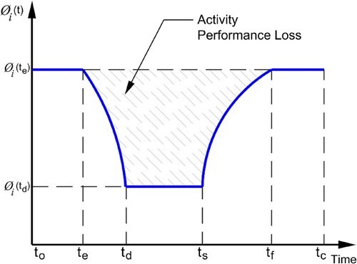
This step takes the SBV approach (discussed in Section 2.2) and, accordingly, measures the resilience of the project activity. This is accomplished by building the resilience curve to model the changes in the availability of the project resources across various stages of disruptive events. Figure 1 provides a schematic illustration of the resilience curve for an activity. In this figure, the horizontal axis represents various stages of disruption, including pre-disruption, disruption, post-disruption degraded, recovery and post-recovery. The vertical axis denotes the performance level of activity $i$ at time $t$, parameterised by ${\mathrm{\varnothing }}_i(t)$.

Figure 1. A schematic representation of the resilience curve.

A resilience curve with the horizontal axis representing various stages of disruption and the vertical axis denoting the performance level of an activity.

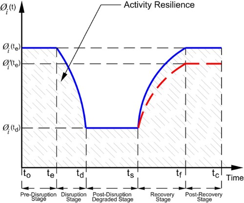
The resilience curve is constructed by projecting the time that a disruptive event strikes the project, the duration of the disruptive event and the changes in the performance level of the activity across various stages of disruption. To measure the performance level of an activity, the ‘probability of success’ indicator is adopted. This enables the establishment of a connection between the availability of project resources, on one hand, and the various stages of disruption on the other. As can be seen from Figure 1, in the pre-disruption stage, the required resources for completing activity $i$ are available (i.e. ${\mathrm{\varnothing }}_i(t_o)={\mathrm{\varnothing }}_i(t_e)=1$), and thus the activity progresses according to the original plan. In the disruption stage, the occurrence of event $e$ at time $t_e$ leads to a drop in the availability of required resources from ${\mathrm{\varnothing }}_i(t_e)=1$ to ${\mathrm{\varnothing }}_i(t_d)<{\mathrm{\varnothing }}_i(t_e)$. In the post-disruption degraded stage, resources are supplied in their degraded states until time $t_s$. During the recovery stage, the project leverages internal resources and/or activates an alternative supply of required resources to fast-track the recovery process. At the end of the recovery stage (time $t_f$), two possible scenarios can take place: (1) resources are available at the same level as at the pre-disruption stage (i.e. ${\mathrm{\varnothing }}_i(t_f)={\mathrm{\varnothing }}_i(t_e)=1$); or (2) the availability of required resources increases, but ${\mathrm{\varnothing }}_i(t_f)<{\mathrm{\varnothing }}_i(t_e)=1$. In fact, quantifying the disruption and recovery profile of an activity, which is visualised by the resilience curve, provides an effective means of understanding how disruption affects the activity. This provides the necessary information for estimating time contingency for this activity.

Building on the resilience curve, the resilience of an activity is now measured by calculating the normalised area of the shaded region in Figure 1. This area lies between the resilience curve and the segment of the horizontal axis bounded between $t_o$ and $t_c$ (Nan and Sansavini 2017). Hence: (2) ${\mathrm{\Psi }}_i=\frac{{\int }_{t_o}^{t_c}{\mathrm{\varnothing }}_i(t)\mathrm{dt}}{t_c-t_o}$(2) where ${\mathrm{\Psi }}_i$ represents the resilience of activity $i$, and $t_c-t_o$ in the denominator of the equation is used to normalise the area underneath the resilience curve.

The resilience curve provides a convenient way to predict the prospective impact of disruptive events on project activities. However, given the considerable uncertainties associated with these events, the resilience curve should be regularly updated as new data evolve over time (Zarghami and Zwikael 2022).

3.3. Step 3: Constructing the progress chart

The progress chart for an activity is created by calculating the fraction of remaining work needed to complete the activity at different time steps (Zarghami 2022b). Figure 2 schematically depicts two progress charts for an activity. The solid line (the solid blue line in the online version) represents the planned progress of the activity over time, and the dashed line (the red dashed line in the online version) denotes the progress of the activity once it has been disrupted. The key elements of the chart are the horizontal axis representing time, the vertical axis showing the fraction of remaining work needed to complete the activity, the planned duration of the activity ($t_{\mathrm{ci}}$), the disrupted duration of the activity ($t{}_{\mathrm{ci}}^{\mathrm{\prime }}$), and the angles between the charts and the horizontal axis (${\theta }_{\mathrm{oi}}$ and ${\theta }_{\mathrm{di}}$).

Figure 2. A schematic illustration of the progress chart.

A typical progress chart with two lines: the solid line representing the planned progress of an activity over time, and the dashed line denoting the progress of the activity once it has been disrupted.

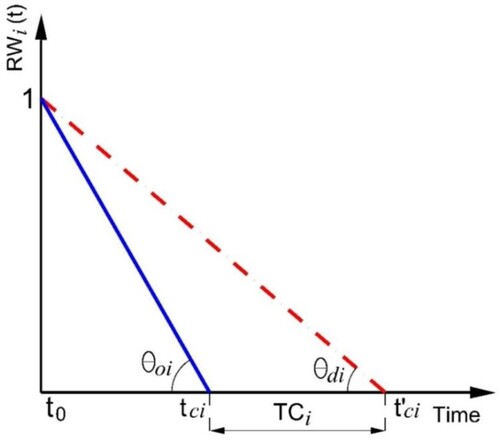
Suppose that at time $t_o$, the fraction of remaining work for activity $i$ is equal to 1. Hence, the fraction of remaining work for this activity at time $t$, denoted by $R{W}_{\mathrm{oi}}(t)$, can be obtained from the following equation: (3) $R{W}_{\mathrm{oi}}(t)=1-\tan ({\theta }_{\mathrm{oi}}).t$(3) where ${\theta }_{\mathrm{oi}}$ represents the angle between the planned progress chart and the horizontal axis, and $\tan ({\theta }_{\mathrm{oi}})$ is defined as the planned progress rate.

In a similar vein, the fraction of remaining work for a disrupted activity can be derived from the following mathematical expression: (4) $R{W}_{\mathrm{di}}(t)=1-\tan ({\theta }_{\mathrm{di}}).t$(4) where $R{W}_{\mathrm{di}}(t)$ parameterises the fraction of remaining work for disrupted activity $i$ at time $t$, ${\theta }_{\mathrm{di}}$ denotes the angle between the disrupted progress chart and the horizontal axis, and $\tan ({\theta }_{\mathrm{di}})$ is defined as the disrupted progress rate.

Using the basic functions of trigonometry for the triangles in Figure 2, we arrive at: (5) $\begin{array}{rl}\tan ({\theta }_{\mathrm{oi}})& =\frac{1}{t_{\mathrm{ci}}}\end{array}$(5) (6) $\begin{array}{rl}\tan ({\theta }_{\mathrm{di}})& =\frac{1}{t{{}^{\mathrm{\prime }}}_{\mathrm{ci}}}\end{array}$(6) Hence: (7) $\frac{t_{\mathrm{ci}}}{t{{}^{\mathrm{\prime }}}_{\mathrm{ci}}}=\frac{\tan ({\theta }_{\mathrm{di}})}{\tan ({\theta }_{\mathrm{oi}})}$(7) The time contingency for activity $i$, parameterised by $T{C}_i$, is defined as the difference between the planned duration and the disrupted duration of the activity. Thus: (8) $T{C}_i=t{{}^{\mathrm{\prime }}}_{\mathrm{ci}}-t_{\mathrm{ci}}=\left(\frac{\tan ({\theta }_{\mathrm{oi}})}{\tan ({\theta }_{\mathrm{di}})}-1\right).t_{\mathrm{ci}}$(8)

3.4. Step 4: Linking resilience to the progress chart

This step links the notion of resilience to the progress of the activity before and after the occurrence of disruptive events. As can be seen from Equation (7)(7) $\frac{t_{\mathrm{ci}}}{t{{}^{\mathrm{\prime }}}_{\mathrm{ci}}}=\frac{\tan ({\theta }_{\mathrm{di}})}{\tan ({\theta }_{\mathrm{oi}})}$(7) , $\tan ({\theta }_{\mathrm{di}})$ and $t{}_{\mathrm{ci}}^{\mathrm{\prime }}$ are inversely correlated. This implies that a relatively low value of $\tan ({\theta }_{\mathrm{di}})$ results in a relatively high duration of disrupted activity. Therefore, the ratio of $\frac{\tan ({\theta }_{\mathrm{di}})}{\tan ({\theta }_{\mathrm{oi}})}$ can be used as an indicator of the losses from disruptions. This concept connects the progress of the activity with the notion of resilience. This is because a low level of losses from disruptions indicates a higher level of activity resilience. The direct correlation between the ratio of $\frac{\tan ({\theta }_{\mathrm{di}})}{\tan ({\theta }_{\mathrm{oi}})}$ and the activity resilience can be captured by the following power function: (9) $\frac{\tan ({\theta }_{\mathrm{di}})}{\tan ({\theta }_{\mathrm{oi}})}={\alpha }_i.({\mathrm{\Psi }}_i{)}^{{\beta }_i}$(9) where ${\alpha }_i$ is the scale parameter with the domain $[0,1]$, ${\beta }_i$ is defined as the shape parameter with the domain $[0,+\mathrm{\infty })$, and ${\mathrm{\Psi }}_i$ represents the activity resilience.

Substituting Equation (9)(9) $\frac{\tan ({\theta }_{\mathrm{di}})}{\tan ({\theta }_{\mathrm{oi}})}={\alpha }_i.({\mathrm{\Psi }}_i{)}^{{\beta }_i}$(9) into Equation (8)(8) $T{C}_i=t{{}^{\mathrm{\prime }}}_{\mathrm{ci}}-t_{\mathrm{ci}}=\left(\frac{\tan ({\theta }_{\mathrm{oi}})}{\tan ({\theta }_{\mathrm{di}})}-1\right).t_{\mathrm{ci}}$(8) results in: (10) $T{C}_i=\left(\frac{1-{\alpha }_i.{({\mathrm{\Psi }}_i)}^{{\beta }_i}}{{\alpha }_i.{({\mathrm{\Psi }}_i)}^{{\beta }_i}}\right).t_{\mathrm{ci}}$(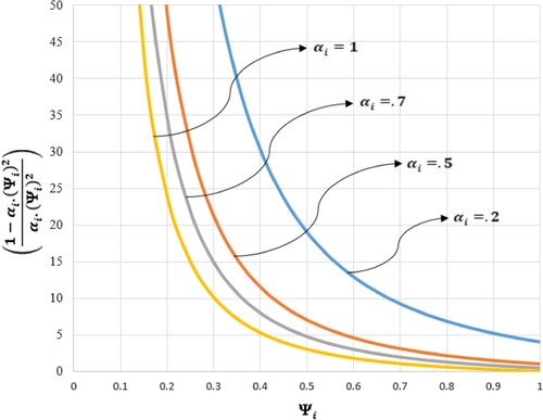10) The scale parameter ${\alpha }_i$ is used to reflect the sensitivity of activity $i$ to the unavailability of its required resources. In fact, the unavailability of a particular resource may represent a more serious issue for some activities than for others. For example, labour-intensive activities, such as hand trenching, are more sensitive to the unavailability of the workforce than equipment-intensive activities, such as pile construction and tunnelling (Gerami Seresht and Fayek 2019). Figure 3 illustrates the changes in the values of $\left(\frac{1-{\alpha }_i.{({\mathrm{\Psi }}_i)}^{{\beta }_i}}{{\alpha }_i.{({\mathrm{\Psi }}_i)}^{{\beta }_i}}\right)$ with respect to different values of ${\alpha }_i$ in which the value of ${\beta }_i$ is held constant (${\beta }_i=2$). As can be observed, a lower value of ${\alpha }_i$ indicates a higher sensitivity to resource unavailability.

Figure 3. The values of $\left(\frac{1-{\mathit{\alpha }}_{\mathit{i}}.{({\mathrm{\Psi }}_{\mathit{i}})}^{{\mathit{\beta }}_{\mathit{i}}}}{{\mathit{\alpha }}_{\mathit{i}}.{({\mathrm{\Psi }}_{\mathit{i}})}^{{\mathit{\beta }}_{\mathit{i}}}}\right)$ with ${\beta }_i=2$ and different values of ${\alpha }_i$.

The changes in the values of with respect to different values of αi in which the value of βi is held constant (βi = 2) where a lower value of αi indicates a higher sensitivity to resource unavailability.

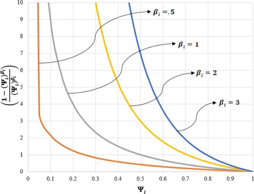
The shape parameter ${\beta }_i$ is used to capture the non-linear relationship between the resilience of activity $i$ and the extent to which this activity is disrupted. Indeed, time contingency increases in a non-linear pattern in relation to the decreasing level of activity resilience. For example, a 20% decrease in the value of the activity resilience does not necessarily lead to a 20% increase in the value of time contingency for the activity. Raising the value of $i$ to the power of ${\beta }_i$ enables us to model this non-linear relationship, thereby estimating time contingencies more accurately. Figure 4 provides a graphical portrayal of the changes in the values of $\left(\frac{1-{\alpha }_i.{({\mathrm{\Psi }}_i)}^{{\beta }_i}}{{\alpha }_i.{({\mathrm{\Psi }}_i)}^{{\beta }_i}}\right)$ with respect to different values of ${\beta }_i$ where the value of ${\alpha }_i$ is held constant (${\alpha }_i=1$). As can be observed, enlarging ${\beta }_i$ will shift the location of the corresponding curve to the right. This implies that an increase/decrease in the value of ${\beta }_i$ leads to an increase/decrease in the value of time contingency.

Figure 4. The values of $\left(\frac{1-{\mathit{\alpha }}_{\mathit{i}}.{{(}_{\mathit{i}})}^{{\mathit{\beta }}_{\mathit{i}}}}{{\mathit{\alpha }}_{\mathit{i}}.{{(}_{\mathit{i}})}^{{\mathit{\beta }}_{\mathit{i}}}}\right)$ with ${\alpha }_i=1$ and different values of ${\beta }_i$.

The changes in the values of with respect to different values of βi where the value of αi is held constant (αi = 1) where enlarging βi will shift the location of the corresponding curve to the right.

Equation (10)(10) $T{C}_i=\left(\frac{1-{\alpha }_i.{({\mathrm{\Psi }}_i)}^{{\beta }_i}}{{\alpha }_i.{({\mathrm{\Psi }}_i)}^{{\beta }_i}}\right).t_{\mathrm{ci}}$(10) yields the value of time contingency for activity $i$ when it is subject to a single disruptive event. Given that project activities are regularly exposed to multiple disruptive events, to accurately estimate time contingency, $T{C}_i$ for all potential disruptive events should be calculated. Considering $q$ different types of disruptive events, the overall time contingency of activity $i$ is computed as the highest value of any time contingency. Hence: (11) $\text{T}{\text{C}}_{\mathrm{iT}}=\text{max }(\text{T}{\text{C}}_{\mathrm{ie}},i=1,2,\dots ,n;e=1,2,\dots ,q)$(11) where index $e$ is used to account for the multiplicity of disruptive events, $\text{T}{\text{C}}_{\mathrm{iT}}$ represents the overall time contingency for activity $i$, $\text{T}{\text{C}}_{\mathrm{ie}}$ denotes the time contingency for activity $i$ when disruptive event $e$ occurs, and $q$ refers to the number of disruptive events.

4. Case studies

This section illustrates and validates the proposed method with two case studies: a real-life construction project and a project taken from the literature. The first case study demonstrates how the proposed method can be used to estimate time contingencies at the work package level. The second case study compares time contingencies at the activity level obtained using the proposed method with that derived from a conventional method using the critical chain project management (CCPM) methodology.

4.1. Case study 1: Numerical illustration

4.1.1. An overview of case study 1

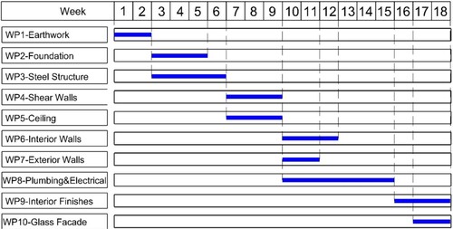
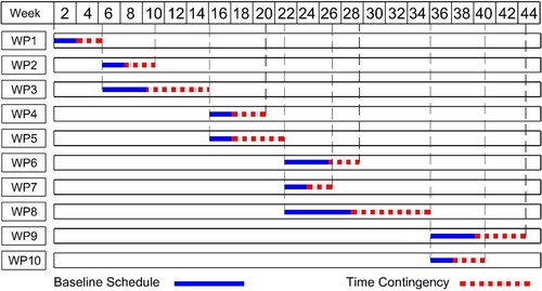
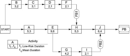
The application of the proposed method is demonstrated in a four-story residential building project. The project involves the construction of an 11 m wide, 22 m long and 0.90 m thick reinforced concrete raft footing. The structural frame is made of steel with concrete slabs and shear walls, with a total floor area of 780 ${\text{m}}^2$. The external and internal walls are, respectively, constructed of 200 and 100 mm thick hollow bricks. Figure 5 illustrates the project network diagram consisting of 10 main work packages. In this figure, the rectangles denote work packages and the arrows illustrate the relationship between work packages. In addition, Figure 6 depicts the Gantt chart (baseline schedule) for the project in which the horizontal bars represent the mean durations of the work packages in weeks. As shown in the Gantt chart, the initial project completion time, before adding time contingencies, is 18 weeks.

Figure 5. Project network diagram (case study 1).

Project network diagram (case study 1) consisting of 10 main work packages in which the rectangles denote work packages and the arrows illustrate the relationship between work packages.

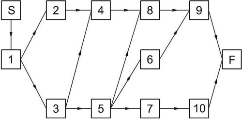
Figure 6. Project Gantt chart (case study 1).

The Gantt chart (baseline schedule) for case study 1 in which the horizontal bars represent the mean durations of the work packages in weeks.

4.1.2. Scenario analysis (case study 1)

A scenario analysis was performed to determine the time contingencies for the case study. To account for the randomness of disruptive events, programme evaluation and review technique (PERT) distribution was used to develop disruption-duration distributions for the pre-disruption, disruption, post-disruption degraded and recovery stages. PERT distribution has been widely used in practice as a computationally expedient technique for estimating the duration of project activities. PERT distribution builds on beta distribution and uses three-point estimation as follows (Sun et al. 2018): (12) ${\text{t}}_E=\frac{t_O+4t_M+t_P}{6}$(12) where $t_E$ represents the expected duration of a specific stage of a disruptive event; and $t_O$, $t_M$ and $t_P$ are, respectively, the minimum, most likely and maximum durations of the specific stage of the disruptive event.

A Monte Carlo simulation was then performed to yield random time durations for the parameters of the PERT distribution in Equation (12)(12) ${\text{t}}_E=\frac{t_O+4t_M+t_P}{6}$(12) . A total of 10,000 replications were run for each stage of the disruptive event, and the average values of these simulation runs were taken as durations of the stage. Table 2 reports the average values of 10,000 simulation runs for the parameters of the PERT distribution corresponding to the two scenarios discussed below.

Table 2. Simulated results for parameters of the program evaluation and review technique (PERT) distribution.

	Scenario 1				Scenario 2
Stage of disruptive event	${\mathit{t}}_{\mathit{O}1}$ ($\times {\mathit{t}}_{\mathit{C}}$)	${\mathit{t}}_{\mathit{M}1}$ ($\times {\mathit{t}}_{\mathit{C}}$)	${\mathit{t}}_{\mathit{P}1}$ ($\times {\mathit{t}}_{\mathit{C}}$)	${\mathit{t}}_{\mathit{E}1}$ ($\times {\mathit{t}}_{\mathit{C}}$)	${\mathit{t}}_{\mathit{O}2}$ ($\times {\mathit{t}}_{\mathit{C}}$)	${\mathit{t}}_{\mathit{M}2}$ ($\times {\mathit{t}}_{\mathit{C}}$)	${\mathit{t}}_{\mathit{P}2}$ ($\times {\mathit{t}}_{\mathit{C}}$)	${\mathit{t}}_{\mathit{E}2}$ ($\times {\mathit{t}}_{\mathit{C}}$)
Pre-disruption	0.16	0.21	0.24	0.207	0.06	0.08	0.19	0.095
Disruption	0.04	0.11	0.14	0.103	0.025	0.055	0.07	0.053
Post-disruption degraded	0.22	0.27	0.49	0.298	0.25	0.48	0.55	0.453
Recovery	0.14	0.17	0.36	0.197	0.05	0.11	0.14	0.105

4.1.3. Results and discussion (case study 1)

Although the proposed method can be used to evaluate the prospective impacts of multiple disruptive events on the project completion time, for illustration purposes, the time contingencies were calculated for two scenarios. The first scenario related to an event that disrupted the supply of required resources. In this scenario, supply shortages led to a 60% decrease in the supply of materials and a 35% reduction in the availability of required equipment. The second scenario referred to a pandemic that struck the project. In line with restrictions imposed by the government, suppliers operated at partial capacity, resulting in a 15% and a 10% capacity reduction in acquiring materials and equipment, respectively. Further, as a result of social distancing restrictions, the number of construction workers onsite at any given time was required to be reduced by 50%.

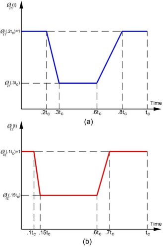
Figure 7(a, b) graph the projected resilience curves corresponding to the first (supply shortages) and second (pandemic) scenarios, respectively. The quantification of the vertical axes in these curves proceeds according to the information on the changes in the availability of resources, as discussed. The horizontal axes show the time spans for various stages of the disruptive events. For example, it can be observed that the post-disruption stage corresponding to the first event (supply shortages) is confined to $0.3t_c$ and $0.6t_c$, whereas it is bounded between $0.15t_c$ and $0.6t_c$ for the second event (the pandemic). For simplicity, the changes in the availability of required resources during the disruption and recovery stages are assumed to be linear. However, depending on the severity of the disruptions and the effectiveness of the corrective actions, different types of degradation and recovery functions, such as exponential and trigonometric, can be employed.

Figure 7. Resilience curves corresponding to two events (case study 1): (a) supply shortages; and (b) a pandemic.

Resilience curves (case study 1) corresponding to: (a) the first scenario (supply shortages); and (b) the second scenario (pandemic). The quantification of the vertical axes in these curves proceeds according to the information on the changes in the availability of resources, as discussed. The horizontal axes show the time spans for various stages of the disruptive events.

Given that construction projects involve labour-intensive activities, the activities in this project are comparatively more sensitive to the disruptions caused by the pandemic than those caused by the supply shortages. Hence, a lower scale parameter value $({\alpha }_{i2}=0.85)$ is considered for the second scenario compared with the first scenario (${\alpha }_{i1}=1$). To capture the non-linear relationship between the resilience of project activities and the extent to which these activities are disrupted, the value of the shape parameter for both scenarios is set as equal to 2 (${\beta }_{i1}={\beta }_{i2}=2$).

Equation (1)(1) ${\mathrm{\varnothing }}_i=\prod _{j=1}^m\left[\sum _{k=K_{\mathrm{ij}}}^{N_{\mathrm{ij}}}\left(\begin{array}{c}{N}_{\mathrm{ij}}\\ K_{\mathrm{ij}}\end{array}\right){a_{\mathrm{ij}}}^k{(1-a_{\mathrm{ij}})}^{(N_{\mathrm{ij}}-k)}\right]$(1) is used to calculate the probability that the project work packages are completed without the interruption caused by the two events: supply shortages and a pandemic. Table 3 reports the numerical values used for determining the time contingencies for the first case study. In this table, $N_{\mathrm{ij}}$ and $K_{\mathrm{ij}}$ are, respectively, the numbers of available and required units of resources, and $a_{i1}$ and $a_{i2}$ represent the probability that resources can be acquired without the interruptions caused by supply shortages and the pandemic, respectively. Further, ${\mathrm{\varnothing }}_{i1}$ and ${\mathrm{\varnothing }}_{i2}$ denote, respectively, the probability of completing work package $i$ without the interruptions caused by supply shortages and the pandemic, and ${\mathrm{\varnothing }}_{i1}$ and ${\mathrm{\varnothing }}_{i2}$, which are obtained from Equation (2)(2) ${\mathrm{\Psi }}_i=\frac{{\int }_{t_o}^{t_c}{\mathrm{\varnothing }}_i(t)\mathrm{dt}}{t_c-t_o}$(2) , indicate the resilience of work package $i$ to the disruptions caused by supply shortages and the pandemic, respectively.

Table 3. The numerical values used for determining time contingencies (case study 1).

Work package $(\mathbf{\text{i}})$	Resource	${\mathit{N}}_{\mathit{ij}}$	${\mathit{K}}_{\mathit{ij}}$	${\mathit{a}}_{\mathit{i}1}$	${\mathit{a}}_{\mathit{i}2}$	${\mathrm{\varnothing }}_{\mathit{i}1}$	${\mathrm{\varnothing }}_{\mathit{i}2}$	$i1$	$i2$
1	Material	3	1	0.4	0.85	0.6880	0.4933	0.8596	0.7340
	Labour	3	2	1	0.5
	Equipment	2	1	0.65	0.9
2	Material	4	2	0.4	0.85	0.3769	0.7203	0.7196	0.8531
	Labour	2	1	1	0.5
	Equipment	3	2	0.65	0.9.
3	Material	1	1	0.4	0.85	0.3059	0.4214	0.6877	0.6962
	Labour	3	2	1	0.5
	Equipment	5	3	0.65	0.9
4	Material	3	2	0.4	0.85	0.3369	0.7038	0.7016	0.8445
	Labour	2	1	1	0.5
	Equipment	3	1	0.65	0.9
5	Material	4	3	0.4	0.85	0.1565	0.4436	0.6204	0.7079
	Labour	3	2	1	0.5
	Equipment	4	2	0.65	0.9
6	Material	1	1	0.4	0.85	0.3829	0.5838	0.7223	0.7815
	Labour	4	2	1	0.5
	Equipment	3	1	0.65	0.9
7	Material	1	1	0.4	0.85	0.2873	0.5680	0.6793	0.7732
	Labour	4	2	1	0.5
	Equipment $r_{72}$	3	2	0.65	0.9
8	Material	2	1	0.4	0.85	0.5591	0.4869	0.8016	0.7306
	Labour	5	3	1	0.5
	Equipment	4	2	0.65	0.9
9	Material	4	3	0.4	0.85	0.1715	0.4448	0.6272	0.7085
	Labour	3	2	1	0.5
	Equipment	3	1	0.65	0.9
10	Material	1	1	0.4	0.85	0.2873	0.4131	0.6793	0.6919
	Labour	3	2	1	0.5
	Equipment	3	2	0.65	0.9

As can be seen in Table 3, the project work packages that are more susceptible to disruptions attain higher values of ${\mathrm{\varnothing }}_i$. This is because the occurrence of disruptive events leads to a decrease in the availability of project resources, and, consequently, reduces the probability of the successful completion of the project work packages. This corroborates the findings of existing studies that have illuminated the significance of resource-based disruptions in contingency planning (Khakifirooz et al. 2023). Specifically, recent studies have cited resource availability as a key factor in forecasting the duration of disrupted activities (Zarghami 2022b).

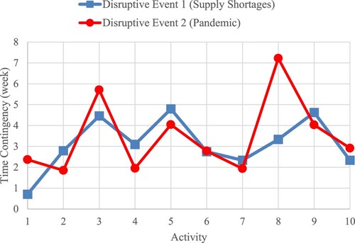
Based on the information provided in Table 3, Equation (10)(10) $T{C}_i=\left(\frac{1-{\alpha }_i.{({\mathrm{\Psi }}_i)}^{{\beta }_i}}{{\alpha }_i.{({\mathrm{\Psi }}_i)}^{{\beta }_i}}\right).t_{\mathrm{ci}}$(10) is used to calculate the time contingencies corresponding to the two disruptive events. Figure 8 provides a visualisation of the resulting values of the time contingencies corresponding to supply shortages and the pandemic. As can be observed, the proposed method yields different values of time contingencies for different disruptive events. For example, when supply shortages are taken into consideration, the time contingency of 3.34 weeks is obtained for work package 8. However, when the pandemic is considered, the time contingency for this work package is estimated to be 7.22 weeks. The considerable difference between these two values can be attributed to the ability of the proposed method to: (1) quantify the disproportionate impact of two disruptive events on project resources; and (2) take account of the disruption and recovery profiles of the project work packages. On one hand, the proposed method discriminates between the negative effects of the two events on project resources; thus, it assigns a lower value of resource availability for the pandemic-related disruption: ${\mathrm{\varnothing }}_{82}=0.4869<{\mathrm{\varnothing }}_{81}=0.5591$. On the other hand, the suggested method considers the disruption and recovery profiles of the work packages by building two different resilience curves for the two events, as illustrated in Figure 7. These two curves reflect two different disruption and recovery profiles, and thus two different values of resilience are derived from these curves: ${}_{82}=0.7306{<}_{81}=0.8016$. This substantiates the findings of prior studies that the concept of resilience can effectively characterise the disruption and recovery profiles of a disrupted project by modelling the changes in the performance of the project over time (Ivanov 2023).

Figure 8. Time contingencies corresponding to supply shortages and a pandemic (case study 1).

The resulting values of the time contingencies corresponding to supply shortages and the pandemic. The considerable difference between these two values is related to the disproportionate impact of two disruptive events on project resources.

Using Equation (11)(11) $\text{T}{\text{C}}_{\mathrm{iT}}=\text{max }(\text{T}{\text{C}}_{\mathrm{ie}},i=1,2,\dots ,n;e=1,2,\dots ,q)$(11) , the higher of the two time contingencies values for supply shortages and the pandemic is taken as the overall time contingency value for each work package. Figure 9 depicts the Gantt chart, including both the baseline schedule and the time contingency for the project activities. As can be observed from this figure, the anticipated project completion time is estimated to be 42.72 weeks. Since the initial project completion time is 18 weeks (as shown in Figure 6), the time contingency of 42.72–18 = 24.72 weeks is estimated. The relatively high value of time contingency for the project can be interpreted as evidence that the two disruptive events can significantly interrupt resource acquisition for the project. Considering the assumptions that supply shortages result in a 60% reduction in the availability of materials and the pandemic reduces the availability of the workforce by 50%, this result is unsurprising. In fact, the proposed method can precisely capture the detrimental impacts of the two events on the project completion time. This indicates that the new method increases the capacity to predict the performance of projects based on the specific impact of each disruptive event, rendering contingency planning more effective. This observation is consistent with the findings of the literature indicating that the incorporation of specific characteristics of disruptive events into contingency planning increases confidence in estimating time contingencies (Zarghami and Zwikael 2023).

Figure 9. Project Gantt chart including baseline schedule and time contingency for the project activities (case study 1).

Project Gantt chart (case study 1) with the anticipated project completion time of 42.72 weeks and the estimated time contingency of 24.72 weeks.

4.2. Case study 2: A comparative analysis

4.2.1. An overview of case study 2

This section compares the proposed method with a case study presented in Zarghami et al. (2020). This study employed the CCPM methodology to determine time contingencies (referred to as ‘time buffers’ therein). CCPM inserts time contingencies, named time buffers, at critical points to minimise variations in the durations of individual activities (Pellerin and Perrier 2019). Accordingly, two types of time contingencies are defined: the project buffer and the feeding buffer. A project buffer is inserted at the end of the critical chain to protect it from delays caused by disruptive events (Moradi and Shadrokh 2019). A feeding buffer is placed at the convergence of the critical chain and the feeding chain to ensure that activities on the feeding chain do not cause any potential delay for activities on the critical chain.

The project network diagram for the second case study is illustrated in Figure 10. As shown in this figure, the network diagram comprises the critical chain $A\to E\to H\to J$ and two feeding chains: the feeding chain $B\to C\to D\to F$ and the feeding chain $G\to I$. Time contingencies were presented in the study as: (1) a project buffer (parameterised by PB in Figure 10), located at the end of the critical chain; and (2) two feeding buffers (parameterised by FB1 and FB2 in Figure 10), positioned at the convergence of two feeding chains and the critical chain.

Figure 10. Critical chain project management (CCPM) network diagram (case study 2).

The CCPM network diagram (case study 2) consisting of the critical chain A → E → H → J and two feeding chains: the feeding chain B → C → D → F and the feeding chain G → I. Time.

Using the CCPM methodology, the time contingency values were obtained from the following equation: (13) $T{C}_{\mathrm{PB}/\mathrm{FB}}=\sqrt{\sum _{i=1}^m{[(2-{\mathrm{\varnothing }}_i)(t_{\mathrm{li}}-t_{\mathrm{ci}})]}^2}$(13) where $T{C}_{\mathrm{PB}/\mathrm{FB}}$ denotes time contingency (PB symbolises the project buffer and FB represents the feeding buffer), ${\mathrm{\varnothing }}_i$ is the probability of the successful completion of activity $i$ without interruption caused by disruptive events, $t_{\mathrm{li}}$ refers to the low-risk duration of activity $i$, and $t_{\mathrm{ci}}$ stands for the mean duration (planned duration excluding time contingency) of activity $i$.

Table 4 reports the time contingency values for the critical chain and the feeding chains using Equation (13)(13) $T{C}_{\mathrm{PB}/\mathrm{FB}}=\sqrt{\sum _{i=1}^m{[(2-{\mathrm{\varnothing }}_i)(t_{\mathrm{li}}-t_{\mathrm{ci}})]}^2}$(13) .

Table 4. Time contingencies for the critical chain and the feeding chains using the CCPM methodology (case study 2).

Symbol	Chain	$\mathit{T}{\mathit{C}}_{\mathit{PB}/\mathit{FB}}$ (week)
PB	$A\to E\to H\to J$	6.1
FB1	$B\to C\to D\to F$	3.82
FB2	$G\to I$	3.08

4.2.2. Results and discussion (case study 2)

To account for the disproportionate impacts of disruptions on project activities, assume that these activities exhibit completely different disruption and recovery profiles. As a result, this section associates a separate resilience curve with each activity. Since space does not permit the presentation of all the resilience curves, the numerical values used for constructing these curves are summarised in Table 5.

Table 5. Numerical values used for constructing the resilience curves for the project activities (case study 2).

Activity	${\mathrm{\varnothing }}_{\mathit{i}}$	${\mathit{t}}_{\mathit{e}}$ (week)	${\mathit{t}}_{\mathit{d}}$ (week)	${\mathit{t}}_{\mathit{s}}$ (week)	${\mathit{t}}_{\mathit{f}}$ (week)	$i$
A	0.70	0.6	0.9	2.1	2.55	0.8425
B	0.55	0.2	0.6	1	1.2	0.8425
C	0.50	0.5	0.8	0.8	1	0.875
D	0.70	0.25	0.45	0.7	0.85	0.8725
E	0.65	1.2	1.8	4.8	6	0.7725
F	0.65	0.65	0.75	0.85	0.9	0.9387
G	0.60	0.4	0.6	1.6	1.8	0.76
H	0.75	0.6	1.35	2.4	3	0.8562
I	0.70	0.4	0.9	0.9	1	0.91
J	0.60	0.4	0.6	3	3.6	0.72

To enable comparisons, Equation (10)(10) $T{C}_i=\left(\frac{1-{\alpha }_i.{({\mathrm{\Psi }}_i)}^{{\beta }_i}}{{\alpha }_i.{({\mathrm{\Psi }}_i)}^{{\beta }_i}}\right).t_{\mathrm{ci}}$(10) is used to determine time contingencies for the critical chain and the feeding chains based on the proposed method. The values of the scale and shape parameters in this equation are set as 1 and 2, respectively. Figure 11 displays the contrast between the time contingencies resulting from the proposed method and the CCPM-based method. As can be seen from this figure, the differences between the resulting values using the two methods are conspicuous. For instance, when the CCPM-based method is applied, $T{C}_{\mathrm{PB}}=6.1\text{weeks}$, whereas the proposed method generates $T{C}_{\mathrm{PB}}=10.1\text{weeks}$. The proposed method yields a longer time contingency for the critical chain than the CCPM-based method because it considers not only the uncertainty in time durations, but also the changes in the availability of project resources over time. In short, as reported in Table 5, activities in the critical chain ($A\to E\to H\to J$) have relatively low levels of resilience. The proposed method captures this point, consequently yielding a longer time contingency for the critical chain compared with the conventional CCPM-based method.

Figure 11. Time contingencies resulting from the proposed and CCPM-based methods (case study 2).

The bar charts displaying the contrast between the values of time contingency resulting from the proposed method and the CCPM-based method.

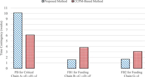
Conversely, the suggested method yields smaller time contingency values for feeding buffers compared with the CCPM-based method. This is related to the ability of the proposed method to provide a complete representation of various stages of disruptive events. That is, the proposed method determines time contingencies by considering information about a drop in the availability of project resources, the restoration of resource availability, the duration of the disruption stage and the speed of recovery. However, the CCPM-based method only accounts for the extent to which the availability of the required resources decreases because of disruptions. In other words, the CCPM-based method focuses exclusively on the drop in the availability of the disrupted resources without considering how long the disruption takes or how fast the recovery is. Consequently, the CCPM-based method overestimates the time contingency value in the case where ${\mathrm{\varnothing }}_i$ is relatively large, but the project regains its performance quickly. The proposed method solves the problem of overestimating time contingency values for feeding buffers, generated by the CCPM-based method, by considering the changes in the availability of resources, as well as the durations of the disruption, post-disruption degraded and recovery stages.

5. Managerial implications

5.1. Implications for delay claims

The history of project management is littered with litigation cases. Many of these cases focus on claims about delay damages. In the process of assessing delay claims, the main task is to evaluate excusable and non-excusable delays. The proposed method can provide the necessary information to distinguish between excusable and non-excusable delays. This can be achieved by quantifying the performance loss of an activity with respect to the availability of its required resources using the resilience curve. Mathematically speaking, the activity performance loss can be quantified by measuring the area of the shaded region that lies between the resilience curve and the segment of the horizontal line $x={\mathrm{\varnothing }}_i(t_e)$ bounded between $t_e$ and $t_f$, where ${\mathrm{\varnothing }}_i(t_e)$ is the value of resource availability before the occurrence of the disruptive event at time $t_e$ (as illustrated in Figure 12). Thus: (14) ${\lambda }_i=1-{\mathrm{\Psi }}_i$(14) where ${\lambda }_i$ is the performance loss of activity ${\mathrm{\Psi }}_i$ due to the disruptive event, and $i$ denotes the activity resilience.

From a practical point of view, project managers can use Equation (1)(1) ${\mathrm{\varnothing }}_i=\prod _{j=1}^m\left[\sum _{k=K_{\mathrm{ij}}}^{N_{\mathrm{ij}}}\left(\begin{array}{c}{N}_{\mathrm{ij}}\\ K_{\mathrm{ij}}\end{array}\right){a_{\mathrm{ij}}}^k{(1-a_{\mathrm{ij}})}^{(N_{\mathrm{ij}}-k)}\right]$(1) (discussed in Step 1, Section 3.1) to forecast the prospective impact of disruptive events on project activities. In the planning phase, the outcome of the first step can be used to construct the initial resilience curve (discussed in Step 2, Section 3.2). As the new data evolve during the execution phase, project managers should iterate back to Steps 1 and 2 to update the resilience curve. Using Equation (13)(13) $T{C}_{\mathrm{PB}/\mathrm{FB}}=\sqrt{\sum _{i=1}^m{[(2-{\mathrm{\varnothing }}_i)(t_{\mathrm{li}}-t_{\mathrm{ci}})]}^2}$(13) , the actual performance loss of the activity can be compared with the projected data on the initial resilience curve. This indicates how well the actual performance loss matches the initial projection, in turn providing evidence about the nature of the delays. For example, in the case where $({\lambda }_i{)}_{\text{actual}}>({\lambda }_i{)}_{\text{projected}}$, a higher-than-expected severity of disruptive event is implied, which can justify the occurrence of an excusable delay. Accordingly, the excusable delay can be obtained from the following equation: (15) $E{D}_i=(T{C}_i{)}_{\text{actual}}-(T{C}_i{)}_{\text{projected}}$(15) where $E{D}_i$ denotes the excusable delay for activity $i$, $(T{C}_i{)}_{\text{actual}}$ represents the updated time contingency obtained from the updated resilience curve and $(T{C}_i{)}_{\text{projected}}$ is the estimated time contingency in the planning phase.

Figure 12. A schematic illustration of activity performance loss on the resilience curve.

The resilience curve showing an activity performance loss. The shaded region that lies between the curve and the segment of the horizontal line x = ∅i(te) bounded between te and tf corresponds to the activity performance loss.

5.2. Implications for resource management

It is generally accepted that an effective resource management plan is a key factor in recovering from disruptions. During disruptive events, the internal resource deployment plan should accommodate disruptions without significant degradation of project performance. In practice, however, leveraging internal resources does not necessarily lead to a successful restoration of project performance. Recovery from a disturbance demands that additional resources be acquired. It is therefore necessary for managers to consider a backup supply of required resources to fast-track the recovery process. However, supply-related decisions may increase the overhead costs in projects (Jaśkowski, Sobotka, and Czarnigowska 2018). For example, supplying backup materials can result in an increase in inventory management costs. This necessitates a resource management plan that recognises the priorities of activities according to their susceptibility to disruptions. The proposed method provides an opportunity to identify such priorities. To achieve this, in the planning phase, managers can use Equation (1)(1) ${\mathrm{\varnothing }}_i=\prod _{j=1}^m\left[\sum _{k=K_{\mathrm{ij}}}^{N_{\mathrm{ij}}}\left(\begin{array}{c}{N}_{\mathrm{ij}}\\ K_{\mathrm{ij}}\end{array}\right){a_{\mathrm{ij}}}^k{(1-a_{\mathrm{ij}})}^{(N_{\mathrm{ij}}-k)}\right]$(1) (discussed in Step 1, Section 3.1) to forecast the susceptibility of project activities to disruptions. That is, if activity $i$ has a low value of ${\mathrm{\varnothing }}_i$, it is likely that this activity will be interrupted by disruptive events. Consequently, a higher priority should be assigned in the resource management plan for an alternative supply of required resources for this activity.

5.3. Simplifying the proposed method for practical application

Most projects involve a large number of activities; however, not all activities are equally important. Some activities are more critical and, thus, require more managerial attention than others (Zarghami 2022a). The literature has developed a variety of indices to evaluate the relative importance of project activities. These indices measure the importance of activities by focusing on various topological and schedule-based parameters, such as the total float of activities, the variations in activity duration, and the interdependency between project activities. Table 6 reports the most quoted indices commonly used for prioritising project activities.

Table 6. An overview of available indices for prioritising project activities.

Index	Parameters	Reference
Criticality index	Total float of activity	Martin (1965)
Significance index	Activity duration	Williams (1992)
	Total project duration
	Total float of activity
	The expected project total duration
Cruciality index	Activity duration	Williams (1992)
	Total project duration
Uncertainty importance measure	Standard deviation of activity duration	Cho and Yam (1997)
	Standard deviation of the total project duration
Schedule sensitivity index	Standard deviation of the activity duration	Vanhoucke (2010)
	Standard deviation of the total project duration
	Total float of activity
Activity importance index	Total float of activity	Zarghami (2022a)
	Standard deviation of activity duration
	Standard deviation of the total project duration
	Eigenvector centrality of activity in the schedule network

To avoid the complexity of the proposed method arising from a large number of project activities, project managers can prioritise activities that are more critical to the timely completion of the project. This can be achieved by using the indices presented in Table 6. To reduce the computational burden, activities with relatively low levels of importance can be aggregated to the work package level. The proposed method can then be applied at the activity level for activities with high levels of importance, while it can be implemented at the work package level for activities with lower levels of importance.

6. Conclusions

This paper has argued that the available studies on contingency planning in projects are open to three lines of criticism: (1) they produced large errors for historically unprecedented disruptions; (2) they overlooked low-probability and high-impact events; and (3) the existing methods yield an unnecessarily large time contingency value for activities with a low level of susceptibility to disruptions, and an insufficiently small time contingency value for activities that are highly susceptible to disruptions. Accordingly, this study developed a method illustrating how the notion of resilience can be framed and measured to enhance contingency planning in projects. The proposed method was applied in two case studies: a four-story residential building project and a case study from the literature. The first case study was selected to demonstrate how the proposed method can be used to estimate time contingencies for prospective disruptions caused by supply shortages and a pandemic, whereas the second case study was used for a comparative analysis of the proposed method with a CCPM-based solution.

The results of the proposed method provide a more accurate estimate of time contingencies because of its ability to: (1) precisely describe what happens when disruption occurs by constructing resilience curves; and (2) measure the disproportionate impact of different disruptive events on different activities by focusing on project resources. In fact, the findings of this research show that to accurately forecast time contingencies, the negative effects of various disruptive events on project activities should be distinguished because different events affect project resources differently. Further, the analysis of the results highlights the dynamic nature of disruptions caused by changes in the availability of resources. As such, this research suggests that the resilience curve be used as an effective means of modelling the dynamics of disruptive events.

To the best of the author’s knowledge, this research is the first to view contingency planning through the lens of resilience; thus, it is hoped that it leads to a shift in the mindset of project management scholars by showing that a risk assessment alone is insufficient for the development of an effective contingency plan. Further, this research has practical implications for the delay analysis of projects. As a result, it can be employed as a decision-support tool for resolving disputes about excusable and non-excusable delays. In addition, the proposed method can be used to prioritise project activities according to their susceptibility to disruptions. This, in turn, can assist project managers in developing cost-effective resource management plans.

This research offers a significant improvement over the existing methods for estimating time contingency; however, much work remains for future studies to address its limitations. The proposed method can be used for the investigation of ‘known unknowns’, where the nature of a disruptive event is known. Future work can be built on this research to develop a method that accounts for the ‘unknown unknowns’, where disruptive events cannot be identified in advance. This may be achieved, for example, by constructing a resilience curve based on the maximum risk capacity of an activity, rather than the impact of disruptions on the activity. Another limitation to be addressed concerns the values of the scale and shape parameters used in Equation (10)(10) $T{C}_i=\left(\frac{1-{\alpha }_i.{({\mathrm{\Psi }}_i)}^{{\beta }_i}}{{\alpha }_i.{({\mathrm{\Psi }}_i)}^{{\beta }_i}}\right).t_{\mathrm{ci}}$(10) . In the absence of empirical evidence, this paper subjectively assumed these values. To increase the accuracy of the proposed method, it would be useful if future research could empirically estimate the values of the scale and shape parameters based on specific characteristics of project activities.

Disclosure statement

No potential conflict of interest was reported by the author(s).

Additional information

Notes on contributors

Seyed Ashkan Zarghami

Dr Seyed Ashkan Zarghami is a Senior Lecturer of Project Management in the Research School of Management at the Australian National University. His research focuses on the development of applied mathematical models with applications to a broad range of fields, including project management, operations management, infrastructure networks, and supply chain management. Ashkan has a great passion for proposing novel ideas and his research appeared in top ranked international journals such as Decision Support Systems, Journal of Construction Engineering and Management, Industrial Marketing Management, Reliability Engineering and System Safety, International Journal of Production Research, IEEE Transactions on Engineering Management, Engineering, Construction and Architectural Management, International Journal of Disaster Risk Reduction, and Systems Research and Behavioral Science. Prior to his academic career, Ashkan worked for several years in large-scale infrastructure network and construction projects.

References

- Cagliano, Anna Corinna, Sabrina Grimaldi, and Carlo Rafele. 2015. “Choosing Project Risk Management Techniques. A Theoretical Framework.” Journal of Risk Research 18 (2): 232–248. https://doi.org/10.1080/13669877.2014.896398.
- Çevikbaş, Murat, Ozan Okudan, and Zeynep Işık. 2022. “New Delay-Analysis Method Using Modified Schedule and Modified Updated Schedule for Construction Projects.” Journal of Construction Engineering and Management 148 (11): 04022119. https://doi.org/10.1061/(ASCE)CO.1943-7862.0002394.
- Charkhakan, Mohammad Hadi, and Gholamreza Heravi. 2018. “Risk Manageability Assessment to Improve Risk Response Plan: Case Study of Construction Projects in Iran.” Journal of Construction Engineering and Management 144 (11): 05018012. https://doi.org/10.1061/(ASCE)CO.1943-7862.0001562.
- Chih, Ying-Yi, Cody Yu-Ling Hsiao, Ali Zolghadr, and Nader Naderpajouh. 2022. “Resilience of Organizations in the Construction Industry in the Face of COVID-19 Disturbances: Dynamic Capabilities Perspective.” Journal of Management in Engineering 38 (2): 04022002. https://doi.org/10.1061/(ASCE)ME.1943-5479.0001014.
- Cho, Jae Gyeun, and Bong Jin Yum. 1997. “An Uncertainty Importance Measure of Activities in PERT Networks.” International Journal of Production Research 35 (10): 2737–2758. https://doi.org/10.1080/002075497194426.
- Dolgui, Alexandre, and Dmitry Ivanov. 2021. “Ripple Effect and Supply Chain Disruption Management: New Trends and Research Directions.” International Journal of Production Research 59 (1): 102–109. https://doi.org/10.1080/00207543.2021.1840148.
- Dolgui, Alexandre, Dmitry Ivanov, and Boris Sokolov. 2018. “Ripple Effect in the Supply Chain: An Analysis and Recent Literature.” International Journal of Production Research 56 (1-2): 414–430. https://doi.org/10.1080/00207543.2017.1387680.
- Elbarkouky, Mohamed M. G., Aminah Robinson Fayek, Nasir B. Siraj, and Naimeh Sadeghi. 2016. “Fuzzy Arithmetic Risk Analysis Approach to Determine Construction Project Contingency.” Journal of Construction Engineering and Management 142 (12): 04016070. https://doi.org/10.1061/(ASCE)CO.1943-7862.0001191.
- Eldosouky, Ibrahim Adel, Ahmed Hussein Ibrahim, and Hossam El Deen Mohammed. 2014. “Management of Construction Cost Contingency Covering Upside and Downside Risks.” Alexandria Engineering Journal 53 (4): 863–881. https://doi.org/10.1016/j.aej.2014.09.008.
- Flyvbjerg, Bent. 2013. “Quality Control and Due Diligence in Project Management: Getting Decisions Right by Taking the Outside View.” International Journal of Project Management 31 (5): 760–774. https://doi.org/10.1016/j.ijproman.2012.10.007.
- Franco-Duran, Diana M., and Jesus M. de la Garza. 2020. “Performance of Resource-Constrained Scheduling Heuristics.” Journal of Construction Engineering and Management 146 (4): 04020026. https://doi.org/10.1061/(ASCE)CO.1943-7862.0001804.
- Gerami Seresht, Nima, and Aminah Robinson Fayek. 2019. “Factors Influencing Multifactor Productivity of Equipment-Intensive Activities.” International Journal of Productivity and Performance Management 69 (9): 2021–2045. https://doi.org/10.1108/IJPPM-07-2018-0250.
- Gunawan, Indra, Frank Schultmann, and Seyed Ashkan Zarghami. 2017. “The Four Rs Performance Indicators of Water Distribution Networks: A Review of Research Literature.” International Journal of Quality & Reliability Management 34 (5): 720–732. https://doi.org/10.1108/IJQRM-11-2016-0203.
- Hammad, Mohammad Wajdi, Alireza Abbasi, and Mike Ryan. 2018. “Developing a Novel Framework to Manage Schedule Contingency Using Theory of Constraints and Earned Schedule Method.” Journal of Construction Engineering and Management 144 (4): 04018011. https://doi.org/10.1061/(ASCE)CO.1943-7862.0001178.
- Holling, C. S. 1973. “Resilience and Stability of Ecological Systems.” Annual Review of Ecology and Systematics 4: 1–23. https://doi.org/10.1146/annurev.es.04.110173.000245.
- Hosseini, Seyedmohsen, and Dmitry Ivanov. 2022. “A New Resilience Measure for Supply Networks With the Ripple Effect Considerations: A Bayesian Network Approach.” Annals of Operations Research 319 (1): 581–607. https://doi.org/10.1007/s10479-019-03350-8.
- Idrus, Arazi, Muhd Fadhil Nuruddin, and Mohammad Arif Rohman. 2011. “Development of Project Cost Contingency Estimation Model Using Risk Analysis and Fuzzy Expert System.” Expert Systems with Applications 38 (3): 1501–1508. https://doi.org/10.1016/j.eswa.2010.07.061.
- Ivanov, Dmitry. 2022. “Lean Resilience: AURA (Active Usage of Resilience Assets) Framework for Post-COVID-19 Supply Chain Management.” The International Journal of Logistics Management 33 (4): 1196–1217. https://doi.org/10.1108/IJLM-11-2020-0448.
- Ivanov, Dmitry. 2023. “Two Views of Supply Chain Resilience.” International Journal of Production Research, Advance online publication. https://doi.org/10.1080/00207543.2023.2253328.
- Ivanov, Dmitry, and Alexandre Dolgui. 2020. “Viability of Intertwined Supply Networks: Extending The Supply Chain Resilience Angles Towards Survivability. A Position Paper Motivated by COVID-19 Outbreak.” International Journal of Production Research 58 (10): 2904–2915. https://doi.org/10.1080/00207543.2020.1750727.
- Ivanov, Dmitry, and Alexandre Dolgui. 2021. “A Digital Supply Chain Twin for Managing the Disruption Risks and Resilience in the Era of Industry 4.0.” Production Planning & Control 32 (9): 775–788. https://doi.org/10.1080/09537287.2020.1768450.
- Ivanov, Dmitry, Boris Sokolov, Frank Werner, and Alexandre Dolgui. 2020. “Proactive Scheduling and Reactive Real-Time Control in Industry 4.0.” Scheduling in Industry 4.0 and Cloud Manufacturing 289: 11–37. https://doi.org/10.1007/978-3-030-43177-8_2.
- Ivanov, Dmitry, Christopher S. Tang, Alexandre Dolgui, Daria Battini, and Ajay Das. 2021. “Researchers’ Perspectives on Industry 4.0: Multi-Disciplinary Analysis and Opportunities for Operations Management.” International Journal of Production Research 59 (7): 2055–2078. https://doi.org/10.1080/00207543.2020.1798035.
- Jaśkowski, Piotr, Anna Sobotka, and Agata Czarnigowska. 2018. “Decision Model for Planning Material Supply Channels in Construction.” Automation in Construction 90: 235–242. https://doi.org/10.1016/j.autcon.2018.02.026.
- Khakifirooz, Marzieh, Michel Fathi, Alexandre Dolgui, and Panos M. Pardalos. 2023. “Scheduling in Industrial Environment Toward Future: Insights from Jean-Marie Proth.” International Journal of Production Research. Advance online publication. https://doi.org/10.1080/00207543.2023.2245919.
- Lerch, Christian M., Heidi Heimberger, A. Jäger, Djerdj Horvat, and Frank Schultmann. 2022. “AI-Readiness and Production Resilience: Empirical Evidence from German Manufacturing in Times of the Covid-19 Pandemic.” International Journal of Production Research, https://doi.org/10.1080/00207543.2022.2141906.
- Li, Hongbo, Xianchao Zhang, Jinshuai Sun, and Xuebing Dong. 2023. “Dynamic Resource Levelling in Projects Under Uncertainty.” International Journal of Production Research 61 (1): 198–218. https://doi.org/10.1080/00207543.2020.1788737.
- Martens, Annelies, and Mario Vanhoucke. 2020. “Integrating Corrective Actions in Project Time Forecasting Using Exponential Smoothing.” Journal of Management in Engineering 36 (5): 04020044. https://doi.org/10.1061/(ASCE)ME.1943-5479.0000806.
- Martin, J. J. 1965. Distribution of the Time Through a Directed, Acyclic Network.” Operations Research 13 (1): 46–66. https://doi.org/10.1287/opre.13.1.46.
- Monzer, Natalie, Aminah Robinson Fayek, Rodolfo Lourenzutti, and Nasir B. Siraj. 2019. “Aggregation-Based Framework for Construction Risk Assessment With Heterogeneous Groups of Experts.” Journal of Construction Engineering and Management 145 (3): 04019003. https://doi.org/10.1061/(ASCE)CO.1943-7862.0001614.
- Moradi, Hadi, and Shahram Shadrokh. 2019. “A Robust Scheduling for the Multi-Mode Project Scheduling Problem With a Given Deadline Under Uncertainty of Activity Duration.” International Journal of Production Research 57 (10): 3138–3167. https://doi.org/10.1080/00207543.2018.1552371.
- Münch, Christopher, and Evi Hartmann. 2023. “Transforming Resilience in the Context of a Pandemic: Results from a Cross-Industry Case Study Exploring Supply Chain Viability.” International Journal of Production Research 61 (8): 2544–2562. https://doi.org/10.1080/00207543.2022.2029610.
- Myers, Albert. 2010. Complex System Reliability: Multichannel Systems with Imperfect Fault Coverage. London, UK: Springer-Verlag.
- Nachbagauer, Andreas, and Iris Schirl-Boeck. 2019. “Managing the Unexpected in Megaprojects: Riding the Waves of Resilience.” International Journal of Managing Projects in Business 12 (3): 694–715. https://doi.org/10.1108/IJMPB-08-2018-0169.
- Naderpajouh, Nader, Juri Matinheikki, Lynn A. Keeys, Daniel P. Aldrich, and Igor Linkov. 2020. “Resilience and Projects: An Interdisciplinary Crossroad.” Project Leadership and Society 1: 100001. https://doi.org/10.1016/j.plas.2020.100001.
- Nan, Cen, and Giovanni Sansavini. 2017. “A Quantitative Method for Assessing Resilience of Interdependent Infrastructures.” Reliability Engineering & System Safety 157: 35–53. https://doi.org/10.1016/j.ress.2016.08.013.
- Negash, Yeneneh Tamirat, and Abdiqani Muse Hassan. 2020. “Construction Project Success Under Uncertainty: Interrelations Among the External Environment, Intellectual Capital, And Project Attributes.” Journal of Construction Engineering and Management 146 (10): 05020012. https://doi.org/10.1061/(ASCE)CO.1943-7862.0001912.
- Pellerin, Robert, and Nathalie Perrier. 2019. “A Review of Methods, Techniques and Tools for Project Planning and Control.” International Journal of Production Research 57 (7): 2160–2178. https://doi.org/10.1080/00207543.2018.1524168.
- Ram, Jiwat. 2023. “Investigating Staff Capabilities to Make Projects Resilient: A Systematic Literature Review and Future Directions.” International Journal of Production Economics 255: 108687. https://doi.org/10.1016/j.ijpe.2022.108687.
- Salah, Ahmad, and Osama Moselhi. 2015. “Contingency Modelling for Construction Projects Using Fuzzy-Set Theory.” Engineering, Construction and Architectural Management 22 (2): 214–241. https://doi.org/10.1108/ECAM-03-2014-0039.
- Steyn, H. 2002. “Project Management Applications of the Theory of Constraints Beyond Critical Chain Scheduling.” International Journal of Project Management 20 (1): 75–80. https://doi.org/10.1016/S0263-7863(00)00054-5.
- Sun, Xiaoguang, R. Houssin, Jean Renaud, and Mickaël Gardoni. 2018. “Towards a Human Factors and Ergonomics Integration Framework in the Early Product Design Phase: Function-Task-Behaviour.” International Journal of Production Research 56 (14): 4941–4953. https://doi.org/10.1080/00207543.2018.1437287.
- Thomé, Antonio Marcio Tavares, Luiz Felipe Scavarda, Annibal Scavarda, and Felipe Eduardo Sydio de Souza Thomé. 2016. “Similarities and Contrasts of Complexity, Uncertainty, Risks, and Resilience in Supply Chains and Temporary Multi-Organization Projects.” International Journal of Project Management 34 (7): 1328–1346. https://doi.org/10.1016/j.ijproman.2015.10.012.
- Vanhoucke, Mario. 2010. “Using Activity Sensitivity and Network Topology Information to Monitor Project Time Performance.” Omega 38 (5): 359–370. https://doi.org/10.1016/j.omega.2009.10.001.
- Vegas-Fernández, Fernando. 2022. “Project Risk Costs: Estimation Overruns Caused When Using Only Expected Value for Contingency Calculations.” Journal of Management in Engineering 38 (5): 04022037. https://doi.org/10.1061/(ASCE)ME.1943-5479.0001064.
- Vegas-Fernández, Fernando, and Fernando Rodríguez-López. 2018. “Methodology for Determining the Most Severe Risks of a Construction Project and Identification of Risky Projects.” Revista de la Construcción 17 (3): 423–435. https://doi.org/10.7764/RDLC.17.3.423.
- Vegas-Fernández, Fernando, and Fernando Rodríguez-López. 2019. “Risk Management Improvement Drivers for Effective Risk-Based Decision-Making.” Pressacademia 8 (4): 223–234. https://doi.org/10.17261/Pressacademia.2019.1166.
- Wied, Morten, Nina Koch-Ørvad, Torgeir Welo, and Josef Oehmen. 2020. “Managing Exploratory Projects: A Repertoire of Approaches and Their Shared Underpinnings.” International Journal of Project Management 38 (2): 75–84. https://doi.org/10.1016/j.ijproman.2019.12.002.
- Wied, Morten, Josef Oehmen, Torgeir Welo, and Ergo Pikas. 2021. “Wrong, but Not Failed? A Study of Unexpected Events and Project Performance in 21 Engineering Projects.” International Journal of Managing Projects in Business 14 (6): 1290–1313. https://doi.org/10.1108/IJMPB-08-2020-0270.
- Williams, Terrie M. 1992. “Criticality in Stochastic Networks.” Journal of the Operational Research Society 43 (4): 353–357. https://doi.org/10.1057/jors.1992.50.
- Zarghami, Seyed Ashkan. 2022a. “Prioritizing Construction Activities: Addressing the Flaws of Schedule-Based Indexes.” Journal of Construction Engineering and Management 148 (8): 04022069. https://doi.org/10.1061/(ASCE)CO.1943-7862.0002328.
- Zarghami, Seyed Ashkan. 2022b. “Forecasting Project Duration in the Face of Disruptive Events: A Resource-Based Approach.” Journal of Construction Engineering and Management 148 (5): 04022016. https://doi.org/10.1061/(ASCE)CO.1943-7862.0002257.
- Zarghami, Seyed Ashkan, Indra Gunawan, Graciela Corral de Zubielqui, and Bassam Baroudi. 2020. “Incorporation of Resource Reliability Into Critical Chain Project Management Buffer Sizing.” International Journal of Production Research 58 (20): 6130–6144. https://doi.org/10.1080/00207543.2019.1667041.
- Zarghami, Seyed Ashkan, and Ofer Zwikael. 2022. “Measuring Project Resilience – Learning from the Past to Enhance Decision Making in the Face of Disruption.” Decision Support Systems 160: 113831. https://doi.org/10.1016/j.dss.2022.113831.
- Zarghami, Seyed Ashkan, and Ofer Zwikael. 2023. “Buffer Allocation in Construction Projects: A Disruption Mitigation Approach.” Engineering, Construction and Architectural Management, https://doi.org/10.1108/ECAM-10-2022-0925.