Adaptive population-based simulated annealing for resource constrained job scheduling with uncertainty

Abstract

Transporting ore from mines to ports is of significant interest in mining supply chains. These operations are commonly associated with growing costs and a lack of resources. Large mining companies are interested in optimally allocating resources to reduce operational costs. This problem has been previously investigated as resource constrained job scheduling (RCJS). While a number of optimisation methods have been proposed to tackle the deterministic problem, the uncertainty associated with resource availability, an inevitable challenge in mining operations, has received less attention. RCJS with uncertainty is a hard combinatorial optimisation problem that is challenging for existing optimisation methods. We propose an adaptive population-based simulated annealing algorithm that can overcome existing limitations of methods for RCJS with uncertainty, including pre-mature convergence, excessive number of hyper-parameters, and the inefficiency in coping with different uncertainty levels. This new algorithm effectively balances exploration and exploitation, by using a population, modifying the cooling schedule in the Metropolis-Hastings algorithm, and using an adaptive mechanism to select perturbation operators. The results show that the proposed algorithm outperforms existing methods on a benchmark RCJS dataset considering different uncertainty levels. Moreover, new best known solutions are discovered for all but one problem instance across all uncertainty levels.

KEYWORDS:

• Resource constrained job scheduling
• uncertainty
• simulated annealing
• adaptive perturbation
• mining

1. Introduction

The mining supply chain in Australia is one of the largest in the world, where a significant proportion of the minerals mined are exported overseas. Mining is major contributor to the Australian economy, with the exporting minerals contributing around $\mathrm{\$}$AUD 200 billion per annum to the economy, employing 240,000 individuals directly, and around 850,000 individuals indirectly.¹ Due to its role in the export of raw materials, Australia has developed a reputation in building mining technologies and is one of the largest suppliers of these technologies and software, worldwide.²

There are numerous problems within the mining supply chain. Of significant interest, is the transportation of ore from mines to ports. In particular, transporting ore from multiple mining sites to a port where resources (trains and trucks) must be shared, is a key problem. If this problem is solved effectively, it can lead to large increases in throughput, thereby leading to substantial gains in revenue for the mining companies. In an abstract form, this problem can be formulated as a resource constrained job scheduling (RCJS) problem. The transportation of ore in batches can be viewed as jobs, while different transport modes (trains or trucks), can be viewed as resources. In the real setting, certain batches are required to be loaded on ships before others, and this aspect can be modelled by precedences between jobs. The timely arrival of ore at the ports is very important, as batches of ore that unnecessarily wait will lead to demurrage costs. This aspect is incorporated as a weighted tardiness for each job (different batches of ore being delayed lead to different costs), and the aim is to ensure the total weighted tardiness across all jobs is kept at minimum.

In the literature, this problem is known as RCJS with a shared central resource (Singh and Ernst 2011; Singh and Weiskircher. 2008; Singh and Weiskircher 2011). The complexity of RCJS makes it challenging for optimisation algorithms, and hence, several approaches have been proposed to tackle it. These include metaheuristics and matheuristics (Cohen et al. 2017; Ernst and Singh 2012; Nguyen et al. 2019; Nguyen and Thiruvady 2020; Nguyen, Zhang, and Chen Tan 2018; Singh and Ernst 2011; Thiruvady, Blum, and Ernst 2020; Thiruvady, Ernst, and Singh 2016; Thiruvady et al. 2012; Thiruvady, Singh, and Ernst 2014). The problem was introduced by Singh and Ernst (2011), who proposed a Lagrangian relaxation based heuristic, which was able to find good solutions and lower bounds. Singh and Weiskircher. (2008) and Singh and Weiskircher (2011) consider a similar problem to RCJS that is modelled as machine scheduling with fractional shared resources. They propose collaborative approaches via agent-based modelling, which prove to be effective in tackling these problems. Ernst and Singh (2012) propose a Lagrangian relaxation based matheuristic that employs particle swarm optimisation, which showed improvements in solution quality across the RCJS benchmark dataset. Thiruvady et al. (2012) consider a variant of RCJS with hard due dates, and they show that an ant colony optimisation (ACO) and constraint programming hybrid can efficiently find feasible and high quality solutions. The study by Thiruvady, Singh, and Ernst (2014) proposes a column generation approach for RCJS, which finds excellent solutions and lower bounds. An inherent issue is the time requirements in solving this problem, and hence, parallel implementations of metaheuristics and matheuristics have been attempted (Cohen et al. 2017; Thiruvady, Ernst, and Singh 2016). The best known solutions for RCJS have been obtained by Nguyen et al. (2019) and Blum et al. (2019). Nguyen et al. (2019) develop a hybrid of differential evolution and column generation, and they show excellent results on small and medium sized problems. Blum et al. (2019) devise a biased random key genetic algorithm, which produces excellent results, especially for large problem instances. In the interest of finding good solutions quickly, studies have shown that genetic programming can be effective for RCJS (Nguyen et al. 2021; Nguyen and Thiruvady 2020; Nguyen, Zhang, and Chen Tan 2018). Finally, Thiruvady, Blum, and Ernst (2020) propose Merge search and CMSA for RCJS.

RCJS under uncertainty (RCJSU) is a variant of RCJS that takes into consideration different practical random sources such as job release times, job processing times or the availability of resources. Of vital importance in RCJS, and crucial in real-world settings, is the uncertain resource availabilities. That is, if trains and trucks breakdown or tracks and roads need maintenance leading to delays in the ore reaching ports, there can be substantial losses incurred. Therefore, planners need a solution method that can address disruptions due to random events to ensure that the solutions obtained can ensure smooth operations either by incorporating uncertainty into optimisation problems, reoptimisation, or reactive dispatching rules. Thiruvady et al. (2022) develop the first RCJSU formulation and propose a surrogate-assisted ant colony system (SACS) to find robust solutions. The results show that SACS outperforms solution methods based on mixed integer programming (MIP), meta-heuristics and surrogate-assisted evolutionary algorithms. Further analyses show that SACS finds good solutions more quickly compared to standard ACO algorithms.

Although SACS has shown promising results, there are some key limitations. Firstly, surrogate models help SACS address the challenge of expensive solution evaluations, but the proposed algorithm tends to converge prematurely, especially for large instances. Therefore, SACS (as well as other existing algorithms in the study of Thiruvady et al. (2022)) can waste a lot of time exploring the search space without making significant progress. Secondly, the proposed method has many pre-defined hyper-parameters such as the learning rate of ant colony systems (ACS) and pre-selection rate for the surrogate models. Because of this issue, the algorithm can have trouble in solving a wide range of instances without major modifications (e.g. reoptimise hyper-parameters). Finally, the performance of SACS is not consistent across different uncertainty levels and different problem sizes (i.e. number of machines). For medium problem sizes and large uncertainty levels, SACS does not show significantly superior performance compared to standard ACS.

This paper addresses the three key limitations discussed above by developing a new adaptive population-based simulated annealing (APSA) algorithm for RCJSU. The two main contributions of this paper are summarised as follows: (1) a new population-based simulated annealing algorithm with a balance between exploration and exploitation and (3) a new adaptive mechanism to update the probabilities for selecting perturbation operators to avoid premature convergence. Additionally, the new efficient simulated annealing algorithm adapts the Metropolis-Hastings method of Singh and Ernst (2011) to converge substantially more quickly by using a faster cooling schedule. APSA is similar to memetic algorithms, and population-based stochastic local search (Hoos and Sttzle 2015; Ong, Hiot Lim, and Chen 2010) that combines evolutionary algorithms and local search heuristics; however, APSA adopts a much smaller population in which the population is improved mainly via local search and adaptive perturbations rather than crossover operators. The balance between exploration and exploitation within APSA allows the algorithms to perform efficiently against noisy and complex problems like RCJSU. Extensive experiments are conducted to validate the superior performance of the proposed algorithms for RCJSU and RCJS.

The paper is organised as follows. Section 2 provides a review of related work. In Section 3, a formulation of the RCJSU problem is provided, including an integer programming model. Section 4 discusses the adaptive population-based simulated annealing algorithm proposed in this study. The experimental evaluation and associated results are presented in Section 5. Section 6 concludes the paper and presents possibilities for future work.

2. Related work

A review of the literature related to RCJS is provided here, including methods and techniques that are effective at tackling problems similar to RCJS and RCJSU.

2.1. Optimisation techniques for tackling RCJS

Owing to the complexity of RCJS, mathematical programming methods on their own do not suffice in finding optimal or even feasible solutions to relatively small problems. Hence, metahuristics and matheuristics have been popular approaches for tackling the problem. Metaheuristics, including partical swarm optimisation (Ernst and Singh 2012), ACO (Thiruvady, Ernst, and Singh 2016), differential evolution (Nguyen et al. 2019), and genetic algorithms (Blum et al. 2019) have been known to find good solutions, albeit with large time overheads. RCJS can be modelled with graphs, and hence, ACO lends itself well to the problem. Nonetheless, past studies on RCJS have shown that ACO tends to converge slowly and gets trapped in local optima. Moreover, diversification strategies including local search (e.g. parallel implementations or niching techniques) help ACO, but the challenges still remain. Hybrid methods, especially those that can guarantee optimality, have also been explored (Nguyen et al. 2019; Singh and Ernst 2011; Thiruvady, Singh, and Ernst 2014), but the results show that only relatively small RCJS problem instances (up to 30 jobs) can be solved with these methods.

2.2. Scheduling on problems with uncertainty

Uncertainty is inherent in many real-world applications, and dealing with uncertainty is often challenging when devising scheduling algorithms. If uncertainty is not considered, the ensuing scheduling algorithms in the deterministic setting are often not effective at even finding feasible solutions (e.g. if a machine breaks down, a job will not be able to start at its pre-determined start time). Hence, a good understanding of the setting in which the schedules are applied is important to ensure success of the scheduling algorithms. Often, reactive scheduling strategies can be more effective in dealing with frequently occurring situations with uncertainties, since the latest information can be incorporated into the decisions. Nonetheless, if predicting the schedules is needed and knowledge of uncertainty is available, the preference is to develop robust schedules. The focus of this paper is on finding robust schedules for RCJSU, since predictable schedules are necessary for mining operations to coordinate supporting activities and to ensure that ore arrives at ports in a timely manner. Of particular interest is the timely arrival of ore at the ports, which relies greatly on the availability of resources. This is indeed the focus in the RCJSU problem and presented in the formulation in Equations (1(1) $\begin{array}{rl}& min\frac{\sum _{s\in \mathcal{U}}\sum _{j\in \mathcal{J}}\sum _{t\in \mathcal{T}}{w}_{\mathrm{jt}}\times (z_{\mathrm{sjt}}-z_{\mathrm{sjt}-1})}{u_s}\end{array}$(1) )–(7(7) $\begin{array}{rlrl}& \sum _{j\in \mathcal{J}}{g}_j\cdot (z_{\mathrm{sj},t+p_j}-z_{\mathrm{sjt}})\le {\mathcal{G}}_s& & \mathrm{\forall }s\in \mathcal{U},\mathrm{\forall }t\in \mathcal{T}L\end{array}$(7) ) (see Section 3).

When tackling scheduling problems with uncertainty, the aim is typically to devise methods that are capable of identifying good solutions under any uncertain scenario. These solutions are called robust solutions and the research area, robust proactive scheduling under uncertainty. There are numerous studies focussing on this area, which we summarise here. Beck and Wilson (2007) investigate job shop scheduling, focussing on a variant which consists of stochastic processing times. They show that hybrids of tabu search and constraint programming with Monte Carlo simulation are effective in handling large-sized problems with uncertainty. Davari and Demeulemeester (2019) develop a branch & bound method and a MIP to tackle the chance-constrained resource-constrained project scheduling problem. The study by Song et al. (2019), proposes branch-and-bound algorithms that generate robust schedules on a variant of resource-constrained project scheduling with processing times that are uncertain depending on time. Ghasemi et al. (2023) propose a mathematical model for a multi-mode resource-constrained project scheduling problem subject to interval uncertainty. Vonder et al. (2006) consider resource-constrained project scheduling with uncertainty by ensuring robustness in start times of the tasks. They develop a heuristic approach to ensure stability in the schedules. Liang et al. (2020) consider bi-objective resource-constrained project scheduling where the aim is to develop schedules with robust resource allocation and time buffering. To tackle the two objectives, they propose a two-stage heuristic method, where simulated annealing is used in the second stage to deal with the time buffers. Identifying robust solutions in uncertain problems introduces additional complexity, and for this purpose metaheuristcs such as swarm intelligence algorithms and evolutionary approaches are known to be effective. Bierwirth and Mattfeld (1999) study genetic algorithms for dynamic job arrivals in classic job shop scheduling. Their results show that their approaches are superior to priority dispatching rules, which are popular in dynamic production scheduling. Wang et al. (2015) devise a surrogate-assisted multi-objective evolutionary method to tackle proactive scheduling where machines are considered to have stochastic breakdowns. To cope with the uncertainty, they propose a job compression and rescheduling strategy (Gao et al. 2019). Support vector regression in conjunction with surrogate models have been proposed to enhance the speed of time-intensive simulations. The study by Wang, Yin, and Jin (2020) provides an in-depth analysis and discussion of scheduling with machine breakdowns. Systematic reviews of scheduling in problems with uncertainty have also been conducted (Chaari et al. 2014; Ouelhadj and Petrovic 2008).

The least two decades have seen numerous studies that consider uncertainty in scheduling problems similar to that of RCJS. There are several similarities to project scheduling, and many studies have considered uncertainty within this setting (Chakrabortty, Sarker, and Essam 2017; Demeulemeester and Herroelen 2011; Herroelen and Leus 2005; Khodakarami, Fenton, and Neil 2007; Lambrechts, Demeulemeester, and Herroelen 2011; Masmoudi and Hait 2013; Moradi and Shadrokh 2019). In these studies, uncertainty is typically considered in respect to the resources, though, a few consider processing time related uncertainty. Lambrechts, Demeulemeester, and Herroelen (2011) study uncertainty with resources, and specifically modes of execution related to the activities. They develop the notion of ‘time buffering’, that efficiently generates robust schedules. Masmoudi and Hait (2013) consider resource levelling and resource constrained project scheduling, and they propose fuzzy modelling to tackle uncertainty. Their solution approaches are a genetic algorithm and a greedy method to identify robust schedules. Khodakarami, Fenton, and Neil (2007) investigate Bayesian networks to identify causal structures considering uncertainty in sources and parameters of a project. They find that Bayesian networks are indeed very effective at dealing with uncertainty, including aspects such as representation, elicitation and management. Uncertainty associated with processing times has also been investigated (Chakrabortty, Sarker, and Essam 2017; Moradi and Shadrokh 2019). Moradi and Shadrokh (2019) develop a problem-specific heuristic to deal with uncertainty and Chakrabortty, Sarker, and Essam (2017) propose several Branch & Cut heuristics for project scheduling.³

2.3. Hybrid optimisation methods

Local search and population-based methods (Luke 2013) have been extensively investigated in the literature to tackle challenging scheduling problems. While local search heuristics are best known for their ability to find local optima efficiently, population-based optimisation methods such as genetic algorithms are better known for their exploration ability. Empirical studies have demonstrated the need to maintain a balance between exploration and exploitation when dealing with difficult combinatorial optimisation problems such as job shop scheduling (Cheng, Gen, and Tsujimura 1999). Such hybrid methods are commonly referred to as memetic algorithms (Ong, Hiot Lim, and Chen 2010) or population-based stochastic local search algorithms (Hoos and Sttzle 2015) in the literature. While hybrid algorithms are effective in combinatorial optimisation, there are still a few shortcomings. Firstly, design choices to develop competitive hybrid algorithms are difficult to make and can be sensitive to different problem subsets. Secondly, the performance of hybrid algorithms depend strongly on an ‘ideal’ setting of the algorithm parameters.

Hybrid algorithms have also been developed for RCJS. The study that introduced the problem (Singh and Ernst 2011) develops a Lagrangian relaxation heuristic, which combines MIP and simulated annealing. Following this, Thiruvady, Singh, and Ernst (2014) show that a column generation and ACO hybrid is very effective on this problem by finding good lower bounds. Parallel implementations of ACO (Thiruvady, Ernst, and Singh 2016) have also been effective, by finding high-quality solutions quickly. Nguyen et al. (2019) propose a hybrid algorithm combining differential evolution and local search, leading to excellent results. The study by Thiruvady, Blum, and Ernst (2020) shows that parallel matheuristics based on MIP and ACO can effectively tackle this problem.

Thiruvady et al. (2022) have developed SACS, a sophisticated algorithm combining ACO, surrogate modelling, and local search to deal with RCJSU. The experiments show that SACS can find excellent solutions for small problems thereby outperforming other meta-heuristics. However, further analyses show that SACS tends to converge prematurely and is inconsistent when working with different problem subsets. Moreover, SACS has many hyper-parameters (for ACO, local search, surrogate models), for which the ideal settings are difficult to find.

3. Problem formulation

Singh and Ernst (2011) propose the original RCJS problem, which is taken directly from the mining industry in Australia. They consider a simplified version of the original problem, which they are able to restate as a job scheduling problem. A major component not considered in RCJS is uncertainty, which is unavoidable in real-world settings. Hence, this study considers this extension to solve what can be considered as closer to the original problem.

The formal definition of RCJSU as an integer program (IP) is provided by Thiruvady et al. (2022). Past studies have considered uncertainty in different ways, including resource limits (Lambrechts, Demeulemeester, and Herroelen 2011) or uncertainty in job/task processing times (Chakrabortty, Sarker, and Essam 2017). However, in this study the focus is on uncertainty derived from the variability in resources, which in turn affects the processing times of jobs/tasks.⁴ The RCJSU problem is NP-hard as it is at least as hard as its deterministic counterpart, which has been shown to be NP-hard by Singh and Ernst (2011). The IP formulation for RCJSU provided by Thiruvady et al. (2022) extends the one for RCJS developed by Singh and Ernst (2011). Uncertainty is introduced by considering several uncertain resource levels, that is, some proportion of the original resource limit is used for each uncertainty sample (details in Section 5.3).

We are given several jobs $\mathcal{J}=\{1,\dots ,n\}$, which are associated with the following information. Each job i has a release time $r_i$, processing time $p_i$, due time $d_i$, weight $w_i$ and resource usage $g_i$, and must execute on machine $m_i$, ($\mathcal{M}=\{1,\dots ,l\}$). Jobs on the same machine cannot execute concurrently, or in other words, only one job may execute at one time. A time horizon is given, consisting of discrete points $\mathcal{T}=\{0,\dots ,D\}$, and D is chosen to be sufficiently large to ensure a feasible solution will always be found. Precendences may exist between any two jobs $i\in \mathcal{J}$ and $j\in \mathcal{J}$ that execute on the same machine. This is represented as $i\to j$, where job i completes before job j starts.

A central resource constraint exists across all machines, where the cumulative resource usage of jobs executing at any time point must be at most $\mathcal{G}$. When considering uncertainty, $\mathcal{G}$ is allowed to vary. This leads to defining a sample, which has available a proportion of the resource $\mathcal{G}$, and is an instance of the problem. As an input, the total number of samples $\mathcal{U}=\{1,\dots ,u_s\}$ is provided, and the resource limit ${\mathcal{G}}_s$ applies to the $s^{\mathrm{th}}$ sample.

The IP can be defined as follows. Let $z_{\mathrm{sjt}}$ be a binary variable, which indicates in sample s, job j completes or has completed by time t, if $z_{\mathrm{sjt}}=1$. By this definition, a job stays complete once completed. Compared to RCJS, the IP formulation for RCJSU requires additional space complexity, which consists of $\mathcal{O}(n^3)$ variables, and each set of constraints with an additional dimension owing to the samples. The IP formulation is: (1) $\begin{array}{rl}& min\frac{\sum _{s\in \mathcal{U}}\sum _{j\in \mathcal{J}}\sum _{t\in \mathcal{T}}{w}_{\mathrm{jt}}\times (z_{\mathrm{sjt}}-z_{\mathrm{sjt}-1})}{u_s}\end{array}$(1) (2) $\begin{array}{rl}& \mathrm{s}.\mathrm{t}.\\ & z_{\mathrm{sj}{t}_{max}}=1& & \mathrm{\forall }s\in \mathcal{U},\mathrm{\forall }j\in \mathcal{J}\end{array}$(2) (3) $\begin{array}{rlrl}& z_{\mathrm{sjt}}-z_{\mathrm{sjt}-1}\ge 0& & \mathrm{\forall }j\in \mathcal{J},\mathrm{\forall }s\in \mathcal{U},\\ & & & t\in \{1,\dots ,t_{max}\}\end{array}$(3) (4) $\begin{array}{rlrl}& z_{\mathrm{sjt}}=0& & \mathrm{\forall }t\in \{1,\dots ,e_j\},\\ & & & \mathrm{\forall }s\in \mathcal{U},\mathrm{\forall }j\in \mathcal{J}\end{array}$(4) (5) $\begin{array}{rlrl}& z_{\mathrm{sbt}}-z_{\mathrm{sa},t-p_b}\le 0& & \mathrm{\forall }(a,b)\in \mathcal{C},\mathrm{\forall }s\in \mathcal{U},\\ & & & \mathrm{\forall }t\in \mathcal{T}\end{array}$(5) (6) $\begin{array}{rlrl}& \sum _{j\in {\mathcal{J}}^i}{z}_{\mathrm{sj},t+p_j}-z_{\mathrm{sjt}}\le 1& & \mathrm{\forall }i\in \mathcal{M},\mathrm{\forall }s\in \mathcal{U},\\ & & & \mathrm{\forall }t\in \mathcal{T}\end{array}$(6) (7) $\begin{array}{rlrl}& \sum _{j\in \mathcal{J}}{g}_j\cdot (z_{\mathrm{sj},t+p_j}-z_{\mathrm{sjt}})\le {\mathcal{G}}_s& & \mathrm{\forall }s\in \mathcal{U},\mathrm{\forall }t\in \mathcal{T}L\end{array}$(7) Equation (1(1) $\begin{array}{rl}& min\frac{\sum _{s\in \mathcal{U}}\sum _{j\in \mathcal{J}}\sum _{t\in \mathcal{T}}{w}_{\mathrm{jt}}\times (z_{\mathrm{sjt}}-z_{\mathrm{sjt}-1})}{u_s}\end{array}$(1) ), the objective function, states that the average total weighted tardiness (TWT) across all samples must be minimised. Constraints (2(2) $\begin{array}{rl}& \mathrm{s}.\mathrm{t}.\\ & z_{\mathrm{sj}{t}_{max}}=1& & \mathrm{\forall }s\in \mathcal{U},\mathrm{\forall }j\in \mathcal{J}\end{array}$(2) ) ensure that all jobs complete. Once a job completes it stays complete, which is enforced by Constraints (3(3) $\begin{array}{rlrl}& z_{\mathrm{sjt}}-z_{\mathrm{sjt}-1}\ge 0& & \mathrm{\forall }j\in \mathcal{J},\mathrm{\forall }s\in \mathcal{U},\\ & & & t\in \{1,\dots ,t_{max}\}\end{array}$(3) ). Constraints (4(4) $\begin{array}{rlrl}& z_{\mathrm{sjt}}=0& & \mathrm{\forall }t\in \{1,\dots ,e_j\},\\ & & & \mathrm{\forall }s\in \mathcal{U},\mathrm{\forall }j\in \mathcal{J}\end{array}$(4) ) ensure that all jobs satisfy release times and the precedences are imposed by Constraints (5(5) $\begin{array}{rlrl}& z_{\mathrm{sbt}}-z_{\mathrm{sa},t-p_b}\le 0& & \mathrm{\forall }(a,b)\in \mathcal{C},\mathrm{\forall }s\in \mathcal{U},\\ & & & \mathrm{\forall }t\in \mathcal{T}\end{array}$(5) ). In this constraint, $e_j=r_j+p_j-1$. Constraints (6(6) $\begin{array}{rlrl}& \sum _{j\in {\mathcal{J}}^i}{z}_{\mathrm{sj},t+p_j}-z_{\mathrm{sjt}}\le 1& & \mathrm{\forall }i\in \mathcal{M},\mathrm{\forall }s\in \mathcal{U},\\ & & & \mathrm{\forall }t\in \mathcal{T}\end{array}$(6) ) require that only one job can execute on one machine at every time point. Constraints (7(7) $\begin{array}{rlrl}& \sum _{j\in \mathcal{J}}{g}_j\cdot (z_{\mathrm{sj},t+p_j}-z_{\mathrm{sjt}})\le {\mathcal{G}}_s& & \mathrm{\forall }s\in \mathcal{U},\mathrm{\forall }t\in \mathcal{T}L\end{array}$(7) ) ensure that the resource limits, considering each sample, are satisfied.

For the RCJS, there are efficient scheduling heuristics that are known (see Section 4.4). These heuristics typically depend on an alternative formulation, where a sequence or permutation jobs are efficiently mapped to schedules. Previous studies have used this approach for RCJS, e.g. Thiruvady, Singh, and Ernst (2014), and it has also proved beneficial for the RCJSU (Thiruvady et al. 2022). In this study, π represents a sequence of jobs while $\sigma (\pi )$ represents an efficient mapping from π to a feasible schedule. Therefore, π is effectively a solution to the problem, where given a sequence, a deterministic schedule can be efficiently constructed.

An example RCJS problem instance is shown in Table 1. This example shows how a solution is constructed and what the optimal solution is. The problem consists of three jobs, with the associated information in the tables. Moreover, the resource capacity is 10 units. Considering π, there are six potential sequences. Among the jobs, the resulting schedules from π will be efficient if Job 3 is scheduled early owing to an early due date and high weight. Additionally, Job 2 should be sequenced before Job 1 due to its higher weight. Given this information, the optimal solution is $\pi =\{3,2,1\}$.

Table 1. An example with 3 jobs and 10 units of resource.

Job	Resource	Weight	Proc.	Due
1	5	0.1	1	2
2	10	0.2	1	2
3	10	0.5	1	1

Note: Proc. is the processing time.

4. Population-based simulated annealing

Several metaheuristics have been able to find excellent solutions to RCJS in a time efficient manner. One of these approaches is simulated annealing (Singh and Ernst 2011). However, to tackle RCJSU, the traditional simulated annealing method has a few shortcomings, and hence, we propose an adaptive population-based simulated annealing (APSA). In particular, this method has three main differences from the traditional approach: (1) a population of solutions to track and exploit best known solutions, (2) a faster cooling schedule within the Metropolis-Hastings algorithm, and (3) adaptive probabilistic selection of the neighbourhood moves to perturb solutions in the population.

The proposed APSA approach is based on the well-known Metropolis-Hastings method, which for an optimisation problem, is known to converge to an optimal solution given infinite time (Granville, Krivanek, and Rasson 1994). As such, the approach proposed here, i.e. APSA, can be expected to exhibit the same characteristics and converge to the optimal solution given infinite time.

4.1. The APSA algorithm

Algorithm 1 shows the high-level APSA procedure for RCJSU. As input, the algorithm takes the following: (a) $T_0$: an initial temperature, (b) $t_{\lim }$: time limit for the execution of the algorithm, (c) Iter: number of Metropolis-Hastings iterations, (d) v: population size, (e) γ: a parameter to control the cooling schedule and (f) ρ: a parameter that specifies how to adapt the probabilities ($\rho =$ 0.9 for this study). In Line 2, the population Π is initialised, where each solution consists of a random list of all the tasks. The best known solution, ${\pi }^{\mathrm{bs}}$, is initialised to be empty. In Line 3, the probability distributions associated with three neighbourhood moves (discussed in the following) are initialised. The main procedure takes place between Lines 4–21, and the algorithm completes execution when the time limit is reached.

Within the main loop, the following is applied to each solution in the population. First, in Line 6, the Metropolis-Hastings algorithm is applied (Algorithm 2) using π as the best solution and for Iter iterations. The resulting solution is stored in ${\pi }^t$. ${\pi }^{\mathrm{bs}}$ is updated to π, if π is an improvement, i.e. $f(\pi )<f({\pi }^{\mathrm{bs}})$. Following this, between Lines 9–19, π is perturbed using a neighbourhood move (details follow in Section 4.3). As part of these steps, the probabilities associated with choosing one of the perturbation moves are adapted or updated. That is, if a move is selected, its corresponding probability reduced by an adaptation factor $\rho =0.9$.

Every solution obtained (by applying any neighbourhood move, etc.) requires the computation of its objective value. As mentioned earlier, a solution is represented by a sequence of the tasks. For each sequence of tasks π, a feasible schedule ($\sigma (\pi )$) is obtained by constructing $u_s$ schedules corresponding to each uncertainty sample. Note, each schedule is resource feasible, ensuring that at most ${\mathcal{G}}_s$ resources are used at each time point for sample s. The result is that each sample has its own TWT. The objective value of π is computed as the average of the TWTs across all samples.

4.2. The metropolis-hastings algorithm

The Metropolis-Hastings method relies on the cooling schedule to ensure a gradual convergence to high-quality regions of the search space. However, due to the overheads introduced by uncertainty, the traditional gradual reduction in temperature will not suffice, and hence we propose a modified version of the method for RCJSU.

Algorithm 2 shows the Metropolis-Hastings procedure. It takes as input: (a) π: current best solution, (b) $T_0$: initial temperature, (c) Iter: number of iterations that the algorithm will execute for and (d) γ: a parameter to determine the cooling schedule. C represents the best known objective value, and is set to a large number. The temperature $T^c$ is set to the initial temperature $T_0$, and the best solution ${\pi }^{\mathrm{ib}}$ is initialised to π. The algorithm executes for Iter iterations (see Lines 3–16 in Algorithm 2). Using ${\pi }^{\mathrm{ib}}$, the neighbourhood move of swapping a pair of jobs is applied. That is, two jobs within the sequence are selected at random and swapped (see Figure 1). If the new solution found ${\pi }^b$ is an improvement, C is updated to the objective value of ${\pi }^b$. Moreover, ${\pi }^{\mathrm{ib}}$ is updated to ${\pi }^b$ and the iteration count is reset. Otherwise, a move to the non-improving solution ${\pi }^b$ is still chosen with probability $e^{-(f({\pi }^{\mathrm{ib}})-C)/T^c}$. The cooling schedule takes place in Line 14.

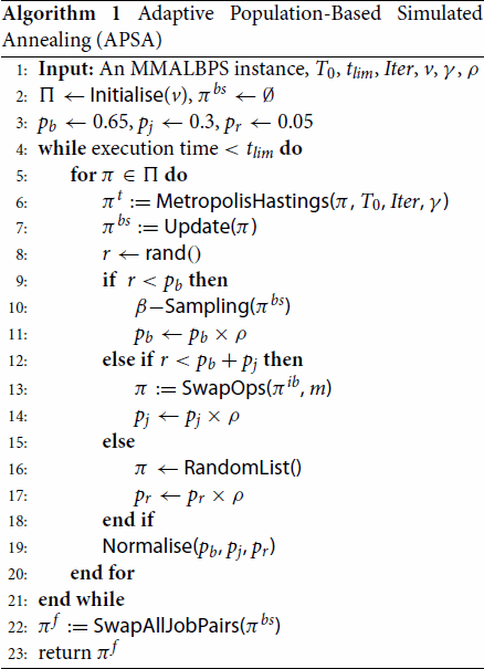
Figure 1. An example that demonstrates job swapping. Two indices are selected randomly, and the corresponding jobs are swapped. In this example, indices 3 and 9 are selected, and the jobs within those indices, 2 and 9, are swapped.

Image of sequence of jobs, followed by applying β-sampling. Five jobs, starting at position 4, are moved to the end of the sequence.

4.3. Adaptive perturbation

Key to the success of APSA is perturbing the best known solution, via three neighbourhood moves. In particular, when applied carefully at different stages of the search, the overall APSA algorithm is able to achieve excellent trade-offs between intensification and diversification.

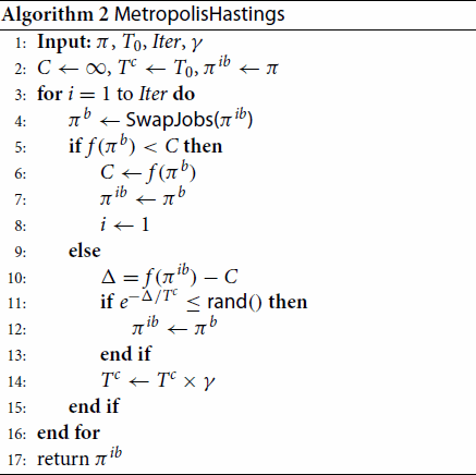
The first neighbourhood move is β-sampling, which is first studied in the context of project scheduling (Valls, Quintanilla, and Ballestin 2003). The basic idea underlying the method is that consecutive jobs or tasks with a sequence are inter-dependent, and moving whole sub-sequences (maintaining certain dependencies) can lead to significant improvements in solutions. For the purposes of the current study, starting at a randomly selected position in the sequence, a sub-sequence of fixed length (5 jobs) is moved to the back of the permutation.

Figure 2 provides an illustration of this method. π consists of 11 jobs. A position $p\in 1,\dots ,n-5$ is chosen randomly, and this sub-sequence (p to p + 5) moves to the end (bottom part of the figure). Here, p = 4, which starts at Job 7, and Jobs 7, 9, 10, 3 and 11 are chosen to move to the end of the sequence. Subsequent jobs (Jobs 8,4, and 5) move up in the sequence to position 4. β-sampling is applied in the above manner in Line 10 of Algorithm 1.

Figure 2. An example that demonstrates β-sampling. From the sequence π, a subset of jobs is selected (7, 9, 10, 3, 11) and moved to the end of the sequence.

Image of sequence of jobs, followed by applying job swapping. Jobs at position 3 and 9, are swapped.

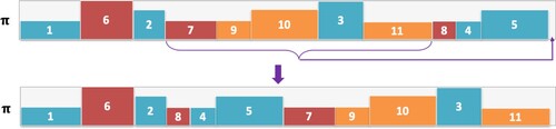
The second neighbourhood move is job swapping. This consists of swapping pairs of jobs in π. Figure 1 shows an example of swapping one pair of jobs. Two positions or indices are chosen at random in the sequence π, and the jobs in these positions are swapped. In the example, Jobs 2 and 8 are swapped.

The third neighbourhood move is to re-initialise the current solution to a randomly chosen sequence. Not surprisingly, the resulting solution can belong to vastly different areas of the search space with a very different objective function value. Hence, this neighbourhood move is expected to produce the largest amount of diversification.

4.3.1. Convergence of probabilities

At each time step, the three neighbourhood moves are selected in a probabilistic manner to perturb the best known solution, with a probability $p_b$ for using β-sampling, $p_j$ for job swapping, and $p_r$ for random re-initialisation, as shown in Algorithm 1. After a neighbourhood move is selected, the probability of selecting the same neighbourhood move in the subsequent step is reduced by a factor of ρ (set to 0.9 in this paper). The probability values $p_b$, $p_j$, and $p_r$, are then normalised such that their sum equals 1. Let $p_b^t$, $p_j^t$ and $p_r^t$ denote the probability values of $p_b$, $p_j$ and $p_r$ at time step t. The following theorem describes the convergence property of the probabilities.

Theorem 4.1

For any initial conditions $p_b^0$, $p_j^0$, and $p_r^0$ within the range of $[0,1]$, subject to the constraint $p_b^0+p_j^0+p_r^0=1$, the probabilities $p_b$, $p_j$, and $p_r$ will eventually converge to the uniform value of 1/3 when time t approaches infinity: (8) $\underset{t\to \mathrm{\infty }}{lim}{p}_b^t=p_j^t=p_r^t=1/3.$(8)

Proof.

Given that the probability values of $p_b$, $p_j$ and $p_r$ at time step t are $p_b^t$, $p_j^t$ and $p_r^t$, the expected probabilities at time step t + 1 can be calculated as (9) $\begin{array}{rl}{p}_b^{t+1}& =p_b^t\left(\frac{0.9p_b^t}{1-0.1p_b^t}\right)+p_j^t\left(\frac{p_b^t}{1-0.1p_j^t}\right)\\ & +p_r^t\left(\frac{p_b^t}{1-0.1p_r^t}\right),\end{array}$(9) (10) $\begin{array}{rl}{p}_j^{t+1}& =p_j^t\left(\frac{0.9p_j^t}{1-0.1p_j^t}\right)+p_r^t\left(\frac{p_j^t}{1-0.1p_r^t}\right)\\ & +p_b^t\left(\frac{p_j^t}{1-0.1p_b^t}\right),\end{array}$(10) (11) $\begin{array}{rl}{p}_r^{t+1}& =p_r^t\left(\frac{0.9p_r^t}{1-0.1p_r^t}\right)+p_b^t\left(\frac{p_r^t}{1-0.1p_b^t}\right)\\ & +p_j^t\left(\frac{p_r^t}{1-0.1p_j^t}\right).\end{array}$(11) Hence the governing differential equations for evolving the probabilities $p_b$, $p_j$ and $p_r$ can be derived: (12) $\begin{array}{rl}\frac{\mathrm{d}{p}_b}{\mathrm{d}t}& =0.1p_b(\frac{p_j^2}{1-0.1p_j}+\frac{p_r^2}{1-0.1p_r}-\frac{p_b(p_j+p_r)}{1-0.1p_b}),\end{array}$(12) (13) $\begin{array}{rl}\frac{\mathrm{d}{p}_j}{\mathrm{d}t}& =0.1p_j(\frac{p_r^2}{1-0.1p_r}+\frac{p_b^2}{1-0.1p_b}-\frac{p_j(p_b+p_r)}{1-0.1p_j}),\end{array}$(13) (14) $\begin{array}{rl}\frac{\mathrm{d}{p}_r}{\mathrm{d}t}& =0.1p_r(\frac{p_b^2}{1-0.1p_b}+\frac{p_j^2}{1-0.1p_j}-\frac{p_r(p_b+p_j)}{1-0.1p_r}).\end{array}$(14) At equilibrium of the differential Equations (12(12) $\begin{array}{rl}\frac{\mathrm{d}{p}_b}{\mathrm{d}t}& =0.1p_b(\frac{p_j^2}{1-0.1p_j}+\frac{p_r^2}{1-0.1p_r}-\frac{p_b(p_j+p_r)}{1-0.1p_b}),\end{array}$(12) )–(14(14) $\begin{array}{rl}\frac{\mathrm{d}{p}_r}{\mathrm{d}t}& =0.1p_r(\frac{p_b^2}{1-0.1p_b}+\frac{p_j^2}{1-0.1p_j}-\frac{p_r(p_b+p_j)}{1-0.1p_r}).\end{array}$(14) ), $\frac{\mathrm{d}{p}_b}{\mathrm{d}t}=\frac{\mathrm{d}{p}_j}{\mathrm{d}t}=\frac{\mathrm{d}{p}_r}{\mathrm{d}t}=0$. Solving this system of equations with $p_b+p_j+p_r=1$, we can obtain the following seven equilibria from the differential equations:

• ($p_b=0,p_j=0,p_r=1$),

• ($p_b=0,p_j=1,p_r=0$),

• ($p_b=1,p_j=0,p_r=0$),

• ($p_b=0,p_j=1/2,p_r=1/2$),

• ($p_b=1/2,p_j=0,p_r=1/2$),

• ($p_b=1/2,p_j=1/2,p_r=0$),

• ($p_b=1/3,p_j=1/3,p_r=1/3$).

However, the first six equilibria are unstable, in the sense that a small disturbance will perturb the system away from those equilibria. The last equilibrium ($p_b=1/3,p_j=1/3,p_r=1/3$) is the only stable equilibrium. Hence, after a sufficient number of time steps, the probability values will converge to this stable equilibrium.

It is worth noting that the decay factor ρ has an impact on the rate at which the probabilities converge, however it does not change the equilibrium state upon convergence. In other words, regardless of the specific value of $\rho \in (0,1)$, the probabilities $p_b$, $p_j$, and $p_r$ will eventually converge to the uniform value of 1/3 given a sufficiently long time. This can be demonstrated by extending the previous proof, wherein we consider a general parameter ρ in the differential equations.

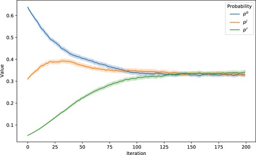
Figure 3 shows a simulation of how the probabilities associated with each neighbourhood move (Algorithm 1) evolve across 200 simulations. We see that three probabilities converge to almost equal levels by 125 simulations.

Figure 3. Adaptive probabilities over 200 simulations.

The convergence profile of of the three adaptive probabilities, pb, pj and pr. We see that all the probabilities converge to approximately 1/3.

4.4. Scheduling heuristic

The aim of the scheduling heuristic is to generate a resource feasible schedule $\sigma (\pi )$ from the sequence π. For this purpose, the serial scheduling scheme is employed (Kolisch 1996), which is adapted from previous studies on RCJS (Singh and Ernst 2011; Thiruvady, Ernst, and Singh 2016; Thiruvady et al. 2012; Thiruvady, Singh, and Ernst 2014). Note, Thiruvady et al. (2022) show that this scheduling scheme can indeed be effective for RCJSU.

The scheduling heuristic works as follows. Jobs in π are selected in the order in which they appear. Each job (j) is tested to see if any of its preceding jobs have not yet been scheduled, and if so, j is placed on the waiting list. Otherwise, j is scheduled as early as possible to ensure that the resource limits are not violated. Once j is scheduled, any job that depends on j (and only j) on the waiting list is scheduled immediately. All such jobs on the waiting list are scheduled in order. Note, for RCJSU, schedules using the procedure above are created for each sample.

Figure 4 shows how the scheduling heuristic works. The problem consists of 15 jobs to be scheduled on three machines. The height of a machine represents the amount of resources available, while a job's height represents its resource requirement. A colour implies a job's machine, i.e. jobs of one colour must go on one machine (e.g. ‘orange’ jobs should be scheduled on machine $m_2$).

Figure 4. An example of a problem with three machines and 15 jobs. From π, jobs are selected in order (left to right) and scheduled on machines that they belong to (e.g. orange jobs on $m_2$). Those jobs that have predecessors that are not yet scheduled will be put on the waiting list $\hat{\pi }$; (a) Job 8 requires Job 2 to be scheduled before it can be scheduled. (b) Job 8 is scheduled once Job 2 has been scheduled, and this will be done as early as possible considering resources.

(a) The figure shows a partial sequence of jobs (π), a waiting list (π^) and three machines (m1,m2,m3). Jobs of the same colour go on the same machine, e.g. blue jobs on machine m1. (b) Job 2 is placed on machine m1 at the first time point where the resources are available. Following this, Job 8 on the waiting list is released, and is also placed in the first available time point on machine m1.

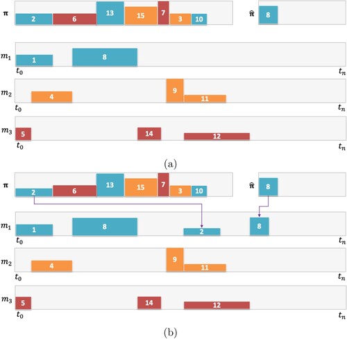
Figure 4(a) shows a permutation π, and a solution that is partially completed with a few jobs allocated to each machine. The waiting list also consists of some waiting jobs $\hat{\pi }$, where for example, Job 8 waits for Job 2 to be scheduled, considering Job 2 precedes Job 8. Figure 4(b) shows one step in the method, where the next job in π, Job 2, is chosen and scheduled in the first available resource feasible time slot on $m_1$. Once Job 2 is scheduled, the waiting list can be examined, and it is found that Job 8 can be released. Job 8 is scheduled as early as possible considering the resource availability.

5. Experiments

A set of experiments and different datasets are applied to fully evaluate the effectiveness and generalisation of the proposed algorithm. We first investigate APSA on RCJSU, and compare its performance to current state-of-the-art approaches, including ACS and SACS.⁵ We further investigate the effect of adaptive population-based approach in APSA by comparing its performance with standard simulated annealing (SA) with the same settings, and the specialised SA proposed in Singh and Ernst (2011). Finally, we examine APSA's performance on the deterministic problem (RCJS), and we compare APSA to ACS, SACS and a column generation and ACO hybrid by Thiruvady, Singh, and Ernst (2014).

5.1. Benchmark datasets

To summarise the RCJS problem, jobs correspond to the transportation of batches of ore, the transport modes (trains or trucks) correspond to resources, and the precedences represent batches of ore that need to arrive at the ports before others. The experiments are conducted on problem instances from the literature.⁶ The problem instances consist 36 randomly generated instances with 3–12, 15 and 20 machines. There are 3 instances per machine size and 10.5 jobs per machine.⁷ The resource usages are defined such that at least two machines may execute at the same time. While this data was originally created for the RCJS, each problem instance is modified to generate the data for RCJSU. Specifically, there are 10 samples generated for each problem instance, where each one has resource limits in the range $[U_{min},U_l\times G]$. $U_{min}$ is chosen to be the largest resource required by any job, i.e. $\underset{i\in \mathcal{J}}{max}{g}_i$, which ensures a resource feasible schedule can always be found. Additionally, the multiplier $U_l\in \{0.5,0.6,0.7,0.8,0.9,1.0\}$ is used to select a proportion of the resources. Typically, a smaller value (e.g. 0.5 or 0.6) means that the problem instance is tightly constrained, where the schedules will need larger completion times, leading to higher overall TWTs.

To gain further insights concerning the strengths of APSA, we investigate a wider range of RCJS problem instances by using the problem generator of Nguyen et al. (2019). The problem instances consider different levels of resource utilisation = [0.25, 0.5, 0.75], number of machines = [3, 4, 5, 6, 7, 8, 9, 10, 12, 15, 18, 20, 25], and the probability of precedences = [0.1, 0.2, 0.3, 0.4, 0.5, 0.6, 0.7 0.8, 0.9]. The resource utilisation indicates how many jobs may execute at the same time, for example, 0.5 indicates that only two jobs may execute at one time. The precedence probability indicates the denseness of the network, where a low probability implies that many jobs can overlap, while a high probability indicates that the jobs will have to be spread out. A total of 1755 problem instances are generated considering seeds, resource utilisation, network complexity and machine size.

5.2. Parameter settings

The parameter settings for APSA are selected through preliminary experimentation, tuning by hand and by using past studies as a guide. We refer to Algorithms 1 and  2. The time limit $t_{\lim }$ is set to 600 seconds. The initial temperature $T_0$ is set to 1500 using Singh and Ernst (2011) as a guide. The parametric experiments in Appendix 1 show that due to uncertainty and the overheads required to construct schedules with a number of samples, the parameters within the Metropolis-Hastings algorithm have to follow a much quicker cooling schedule. This is achieved by allowing only 1000 iterations (Iter = 1000) and $\gamma =0.5$. Moreover, experiments regarding population size in Appendix 1 show that v = 10 is a reasonable choice. The sub-sequence size used within β-sampling of length 5 jobs, which is obtained from Singh and Ernst (2011). Moreover, in Line 14 of Algorithm 1, there are $m=\mathrm{rand}()\ast n$ applications of job swapping, where $\mathrm{rand}()$ is a random number between 0 and 1. The parameter settings for ACS and SACS are obtained from Thiruvady et al. (2022), to which we refer the reader for complete details.

We carry out experiments on all problem instances considering all uncertainty levels. There are 25 repetitions of for each algorithm, with each one given 10 min of wall clock time. The memory limit was 2 GB, which proved to be sufficient for all algorithms. The algorithms were implemented in C++ with GCC-5.4.0. All experiments were carried out on Monash University's Campus Cluster – MonARCH.⁸

The IP was implemented in Gurobi 9.0.1 (Optimization 2010). It was run for 10 min per problem instance and allowed a larger amount of memory of 10GB. Across all the runs, only one solution was found for one problem instance at the uncertainly of 0.8. This is not surprising given the size of the model, which is unsuitable in practical settings. Note, consider for example the IP model for an instance with 20 machines. The integer program for this problem instance consists of over 6.9 million decision variables, over 11.4 million constraints and over 49.3 million non-zeros. The size of this IP is clearly far too large to be able to provide meaningful solutions to RCJSU.

5.3. Comparison between APSA and the state-of-the-art

The results that follow are reported as a percentage difference from the best solution quality found by each algorithm averaged over 25 runs to the best solution found by any algorithm. Consider a problem instance and let $B\ast$ be the best solution obtained by any algorithm for that problem instance. Let $A_k$ be the best solution found by APSA for instance k averaged across 25 runs. Then the percentage difference for APSA is $\frac{A_k-B\ast }{A_k}\times 100\mathrm{\%}$.

Tables 2 and 3 show the results of ACS, SACS and APSA for low and high uncertainty levels (UL), respectively. The tables show the best result obtained by any algorithm (which is highlighted in bold if it is found by APSA) for each uncertainty level, followed by the percentage differences of each algorithm to the corresponding best solution. The best result found by any algorithm for a problem instance is highlighted in bold. Moreover, statistical tests were performed using a Wilcoxon ranked-sum test, and the statistically significant results are marked with a ‘*’. To summarise the performance of the algorithms across the problem instances, the last row of the tables reports the number of times (# best) an algorithm finds the best solution.

Table 2. Results of ACS, SACS and APSA shown as the percentage difference to the best solution for uncertainty levels 0.5, 0.6 and 0.7; Results in column ‘Best’ are highlighted in bold if APSA finds the best solution; Results for each algorithm are highlighted in bold when they achieve best average results, while statistically significant results (pair-wise Wilcoxon ranked-sum test) at a 95$\mathrm{\%}$ confidence interval are marked with a *.

	Uncertainty Level 0.5				Uncertainty Level 0.6				Uncertainty Level 0.7
Instance	Best	ACS	SACS	APSA	Best	ACS	SACS	APSA	Best	ACS	SACS	APSA
3–5	971.7	1.034	1.043	*0.142	942.6	0.494	0.404	*0.048	988.8	1.177	1.092	*0.260
3–23	224.9	0.934	0.791	*0.000	232.5	2.314	2.052	*0.138	240.5	2.374	2.345	*0.162
3–53	221.5	0.474	0.366	*0.000	213.4	0.066	0.028	−0.005	231.7	0.319	0.211	*0.000
4–28	150.6	6.754	6.768	*0.671	128.1	6.409	6.300	*1.046	116.1	6.763	6.720	*0.164
4–42	401.7	1.327	1.279	*0.144	361.1	1.603	1.606	*0.219	323.9	0.540	0.509	*0.034
4–61	248.3	5.578	5.324	*0.209	213.2	4.877	4.192	*0.225	196.6	8.246	7.519	*1.073
5–7	801.3	3.582	3.590	*0.604	673.3	4.496	4.147	*0.371	656.6	3.925	3.932	*0.801
5–21	683.6	4.640	4.353	*1.066	535.8	6.148	5.088	*0.649	577.4	5.504	4.342	*1.320
5–62	816.7	4.660	4.450	*0.579	688.0	5.712	5.436	*1.145	676.5	5.117	5.175	*1.042
6–10	1971.2	4.115	3.230	*0.859	2026.3	4.708	3.944	*1.610	1583.3	5.018	4.215	*1.520
6–28	739.3	5.201	5.212	*0.587	762.4	5.105	4.963	*1.229	574.8	6.738	6.692	*1.541
6–58	763.9	4.778	4.590	*1.468	799.0	4.781	4.303	*1.055	587.2	6.391	6.214	*0.823
7–5	1235.3	2.203	2.054	*0.131	1025.5	3.745	3.631	*0.725	1213.8	2.963	2.833	*0.386
7–23	1426.7	6.619	5.917	*1.641	1194.3	6.363	6.007	*1.776	1391.4	6.034	5.365	*1.286
7–47	1442.1	6.778	5.901	*1.540	1191.5	6.496	5.815	*1.461	1410.3	6.524	5.664	*1.529
8–3	1856.4	10.401	7.545	*1.670	1995.5	10.389	8.257	*2.845	1640.1	11.968	9.434	*3.054
8–53	1154.1	6.363	6.101	*1.623	1250.5	5.754	5.576	*1.181	1053.8	6.512	6.794	*1.839
8–77	2799.0	5.864	4.565	*1.612	2971.5	5.134	4.193	*1.135	2570.1	5.883	5.522	*2.000
9–20	2462.6	5.900	5.301	*1.648	2086.1	5.375	5.114	*1.227	2125.4	5.644	5.402	*1.836
9–47	3185.0	6.684	5.270	*2.029	2640.4	7.618	5.934	*1.993	3333.7	6.529	5.134	*2.123
9–62	3485.6	4.678	4.103	*1.154	2969.1	4.414	3.864	*0.869	3656.7	4.199	3.589	*1.060
10–7	5854.2	4.066	3.749	*0.875	5603.8	4.764	4.108	*1.387	5126.2	4.792	4.332	*1.198
10–13	5246.0	3.092	2.783	*0.769	4932.8	4.675	4.018	*1.607	4517.0	4.719	4.497	*1.694
10–31	1603.1	6.196	6.914	*1.724	1525.3	6.018	6.445	*1.210	1369.6	6.959	7.841	*1.608
11–21	2359.0	4.747	5.053	*1.167	2402.8	4.731	4.919	*0.990	2502.8	5.099	4.934	*1.247
11–56	3991.0	4.836	4.420	*1.185	4047.3	5.072	4.196	*1.177	4156.7	5.714	5.204	*2.094
11–63	4354.2	3.885	3.518	*0.863	4196.9	5.211	4.887	*1.682	4561.3	3.580	3.516	*0.636
12–14	4405.2	4.136	4.295	*1.429	4378.3	4.937	4.890	*1.944	3636.3	4.592	4.533	*1.352
12–36	6825.5	2.979	3.217	*1.484	6844.5	3.762	3.376	*1.435	5710.1	3.732	3.504	*1.429
12–80	5234.4	6.105	5.769	*2.985	5310.1	4.949	4.875	*2.004	4460.8	5.080	4.653	*2.376
15–2	8105.5	3.879	4.319	*3.304	7577.1	3.058	3.153	*2.565	7737.2	2.834	2.843	*2.015
15–3	9206.1	4.375	4.181	*2.511	8585.2	3.669	3.626	*2.008	8820.9	2.820	2.663	*0.972
15–5	7548.8	5.099	5.345	*2.547	7021.0	4.965	4.958	*2.430	7186.8	3.964	3.968	*1.876
20–2	15,042.1	2.994	3.320	*1.635	14,021.9	2.747	2.957	*1.928	15,724.6	2.889	2.738	*1.793
20–5	25,172.0	3.239	2.917	*1.693	23,175.3	3.832	4.185	*2.425	26,028.0	3.782	4.010	*2.558
20–6	13,733.3	2.596	2.678	*1.614	12,713.5	2.707	2.725	*1.900	14,329.1	2.554	2.630	*1.713
$\mathrm{\#}$ best	–	0	0	36	–	0	0	36	–	0	0	36

Table 3. Results of ACS, SACS and APSA shown as the percentage difference to the best solution for uncertainty levels 0.8, 0.9 and 1.0; Results in column ‘Best’ are highlighted in bold if APSA finds the best solution; Results for each algorithm are highlighted in bold when they achieve best average results, while statistically significant results (pair-wise Wilcoxon ranked-sum test) at a 95$\mathrm{\%}$ confidence interval are marked with a *.

	Uncertainty Level 0.8				Uncertainty Level 0.9				Uncertainty Level 1.0
Instance	Best	ACS	SACS	APSA	Best	ACS	SACS	APSA	Best	ACS	SACS	APSA
3–5	861.9	0.972	0.773	*0.031	949.2	0.165	0.162	*0.000	786.3	0.424	0.439	*0.050
3–23	214.6	1.981	1.631	*0.084	232.2	1.636	1.666	*0.000	200.9	2.787	2.568	*0.244
3–53	186.0	0.016	0.016	*0.000	212.5	0.085	0.047	*0.000	145.5	0.069	0.041	*0.000
4–28	101.5	7.224	6.800	*0.857	113.3	4.556	4.830	*0.618	64.5	8.632	8.368	*1.364
4–42	279.3	1.891	1.457	*0.329	300.6	0.935	0.975	*0.116	212.4	2.241	1.973	*0.009
4–61	168.7	7.753	7.327	*0.854	186.6	6.062	5.729	*1.388	114.9	6.922	6.983	*1.654
5–7	573.2	4.079	3.704	*0.406	632.9	4.775	4.399	*0.242	589.9	4.582	3.841	*0.071
5–21	445.1	5.687	5.028	*1.654	488.2	5.930	4.931	*1.540	505.9	5.582	4.556	*1.044
5–62	575.7	6.429	5.659	*1.553	645.9	6.114	5.526	*1.118	592.3	5.185	4.788	*1.047
6–10	1880.3	4.587	3.369	*0.899	1404.6	5.327	4.447	*1.101	1674.6	3.967	3.259	*0.809
6–28	702.7	6.215	5.974	*1.083	502.2	6.283	6.263	*1.296	598.6	5.578	5.366	*0.984
6–58	736.0	4.356	3.806	*1.067	517.5	6.059	5.606	*1.015	794.9	4.651	3.495	*0.742
7–5	992.0	3.793	3.876	*0.812	1277.6	2.216	2.062	*0.272	919.6	4.071	3.771	*1.075
7–23	1163.8	6.092	5.997	*1.662	1466.6	5.974	5.281	*1.206	1058.8	7.126	6.215	*1.327
7–47	1135.7	7.691	6.703	*2.246	1493.3	6.067	5.524	*1.051	1031.0	8.798	7.950	*2.866
8–3	1594.1	10.686	8.116	*2.517	1740.7	9.527	7.545	*1.922	1077.0	13.622	10.734	*2.893
8–53	1041.5	6.370	5.954	*1.625	1107.4	5.501	5.821	*1.518	752.1	7.790	7.627	*2.153
8–77	2499.8	5.215	4.627	*1.302	2669.8	4.973	4.097	*1.163	1861.2	6.300	4.572	*1.253
9–20	2277.7	5.016	4.463	*1.343	1964.0	5.258	5.149	*1.170	1959.1	6.745	6.119	*2.360
9–47	2868.8	6.328	4.602	*1.956	2048.5	6.802	5.562	*1.512	2312.4	6.872	5.587	*1.624
9–62	3189.2	4.428	4.091	*1.275	2316.4	5.602	4.744	*1.526	2609.0	4.345	3.926	*0.947
10–7	4216.6	5.468	5.133	*2.104	4675.7	4.641	4.449	*1.545	4010.0	5.551	5.095	*1.859
10–13	3721.5	4.347	4.032	*1.152	4107.9	4.741	4.474	*1.548	3522.7	4.906	4.490	*1.417
10–31	1100.6	8.086	8.739	*1.873	1249.2	5.754	6.423	*1.094	1041.7	6.940	7.985	*1.382
11–21	1948.8	5.689	5.640	*1.829	1940.4	5.596	5.714	*1.757	2050.3	5.098	4.992	*1.648
11–56	3322.7	5.332	4.479	*1.307	3291.5	5.616	5.364	*1.741	3452.8	4.922	4.790	*1.473
11–63	3504.1	4.215	4.112	*1.296	3312.6	4.210	4.106	*1.008	3670.2	3.747	3.788	*0.900
12–14	3625.5	4.608	4.575	*1.365	2998.5	4.821	5.534	*1.807	2781.7	6.100	5.753	*2.273
12–36	5705.1	3.695	3.216	*1.549	4798.6	4.066	3.667	*1.820	5923.6	3.240	3.124	*1.236
12–80	4447.2	5.204	4.647	*2.377	3754.3	5.471	5.201	*2.299	3534.2	5.557	5.138	*2.620
15–2	6311.7	2.411	2.192	*1.555	7051.6	3.569	3.568	*3.032	5905.5	2.888	2.977	*2.104
15–3	7074.2	3.101	3.040	*1.102	8037.3	2.679	2.814	*1.449	6630.9	3.497	3.397	*1.511
15–5	5753.9	4.440	4.115	*1.766	6473.3	6.295	5.637	*3.051	5431.4	4.227	4.047	*1.682
20–2	13,838.7	3.476	3.375	*2.390	13,081.1	2.433	2.402	*1.347	12,956.3	3.272	3.372	*2.110
20–5	22,944.5	4.050	3.861	*2.593	21,584.8	3.658	3.912	*2.586	21,684.4	2.997	2.975	*1.512
20–6	12,518.9	3.399	3.142	*2.205	11,895.5	1.884	2.172	*1.169	11,880.4	1.851	1.780	*1.014
$\mathrm{\#}$ best	–	0	0	36	–	0	0	36	–	0	0	36

The results in both tables demonstrate the efficacy of our proposed APSA algorithm when compared against two state-of-the-art algorithms, ACS and SACS. The APSA consistently generates the best-known solutions across all problem instances with various levels of uncertainty, with only one exception on instance 15-2 under an uncertainty level of 0.9. Remarkably, the best solutions found by APSA averaged across 25 independent runs are statistically significantly better than those generated by ACS and SACS.

Upon a closer look, we observe that the superiority of APSA over the other two algorithms is less significant when dealing with the smallest (3-machine) and largest (20-machine) problem instances. Regarding the cases with 3 machines, this outcome is not surprising, given the simplicity of these small problem instances which all algorithms are expected to solve optimally or near-optimally. For the large problem instances with 20 machines, the performance of APSA is hindered by the relatively limited number of iterations (less than 10) that APSA can perform within the cutoff time. As a result, APSA has not well converged in these cases, resulting in less notable improvements when compared to the enhancements seen in other instances.

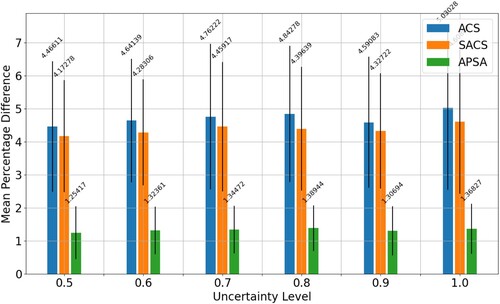
The results in Tables 2 and 3 are summarised in Figure 5. This figure shows how each algorithm (ACS, SACS, and APSA) performs across different uncertainty levels. The bars in the figure indicate the percentage difference from the best result averaged across all instances within a given uncertainty level. This figure clearly demonstrates that our proposed APSA algorithm significantly outperforms the two state-of-the-art methods across all uncertainty levels.

Figure 5. The figure shows a bar chart of the performance of ACS, SACS and APSA. It shows the average percentage difference to best (y-axis) for each uncertainty level (x-axis). We see that APSA has a distinct advantage across all uncertainty levels.

A comparison of ACS, SACS and APSA across six uncertainty levels. There is a clear advantage of APSA over the other two methods.

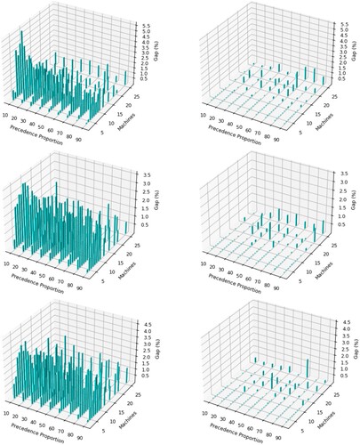
We now consider the additional problem instances using the problem generator of Nguyen et al. (2019). Figure 6 shows the results for uncertainty level 0.6 and resource utilisations of 0.25$\mathrm{\%}$ (top), 0.5$\mathrm{\%}$ (middle) and 0.75$\mathrm{\%}$ (bottom), averaged across five seeds. The z-axis shows Gap as a percentage, which is the gap from either SACS (left) or APSA (right) (B) to the best solution obtained by APSA or SACS ($b^{\ast }$) (Gap $\mathrm{\%}$ = $(B-b^{\ast })/b^{\ast }$). A gap of 0 implies that the algorithm finds the best solution. We see that irrespective of the amount of resource utilisation, APSA significantly outperforms SACS. The gaps usually increase with lower proportion of precedences. Interestingly, with increasing machine size, APSA on rare occasions is outperformed by SACS, but these are for relatively few problem instances. On close examination of the results, we find for the large problem instances, that very few iterations of SA are performed, thereby rendering the adaptive component ineffective.

Figure 6. A comparison of SACS (left) and APSA (right) for RCJSU at uncertainty level 0.6 considering varying levels of resource utilisation (top = 0.25$\mathrm{\%}$, middle = 0.5$\mathrm{\%}$, bottom = 0.75$\mathrm{\%}$), machine sizes and precedence proportion. Gap $\mathrm{\%}$ = $(B-b^{\ast })/b^{\ast }$, where B is APSA or SACS and b* is the best solution.

A comparison of SACS and APSA considering problem characteristics including precedence proportion, resource utilisation and number of machines for uncertainty level 0.6.

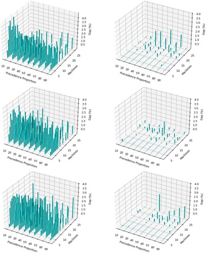
Figure 7 shows the results for uncertainty level 0.9, and is similar to Figure 6. The results show a similar pattern to Figure 6, where overall, APSA significantly outperforms SACS. In similar fashion, the gaps increase with lower proportion of precedences, and SACS's performance improves on a very few problem instances when machine sizes get bigger. We note that the time allowance of 10 min for a single run can be limiting, especially for instances with 20 or more machines, and providing larger time allowances (e.g. 1 hour is reasonable in practical settings) can lead to substantial gains. Interestingly, some of the gaps are higher for uncertainty level 0.9 compared to 0.6, especially for low resource utilisation, implying that for less constrained problems and more room to utilise resources, APSA is the best solution.

Figure 7. A comparison of SACS (left) and APSA (right) for RCJSU at uncertainty level 0.9 considering varying levels of resource utilisation (top = 0.25$\mathrm{\%}$, middle = 0.5$\mathrm{\%}$, bottom = 0.75$\mathrm{\%}$), machine sizes and precedence proportion. Gap $\mathrm{\%}$ = $(B-b^{\ast })/b^{\ast }$, where B is APSA or SACS and $b^{\ast }$ is the best solution.

A comparison of SACS and APSA considering problem characteristics including precedence proportion, resource utilisation and number of machines for uncertainty level 0.9. There is a clear advantage for APSA on small and medium sized problems and a small advantage on large problems.

The strength of our proposed APSA approach lies in its ability to strike a strong balance between diversification and convergence. The simulated annealing component, on one hand, concentrates on the local improvement of solutions, which helps with convergence. On the other hand, keeping a population of solutions prevents the search from getting trapped in a local optimum, effectively enhancing the diversity of the search.

5.4. Convergence characteristics of APSA

We examine the convergence of APSA, and compare it to ACS and SACS. We choose four problem instances, which are sufficiently diverse in size to allow making somewhat general inferences about APSA. The results are shown in Figure 8, where each sub-figure corresponds to one problem instance. The plots show time in seconds on the x-axis and TWT (logarithmic scale) on the y-axis.

Figure 8. Convergence profiles of ACS, SACS and APSA on four RCJSU problem instances of different sizes. The instances chosen are 3–53, 6–28, 9–47 and 12–14. The TWTs on the y-axes are presented on a logarithmic scale.

Each figure compares ACS, SACS and APSA for a single run for the problem instances 3–53, 6–28, 9–47 and 12–14. We see how APSA is able to find higher quality solutions early, and due to the adaptive probabilities, it is able to continue to improve across a run for all problem instances.

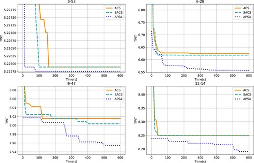
Again, APSA is clearly the best performing method across all four problem instances. There are two main advantages of the algorithm, especially related to the population and diversification. Firstly, the starting solution, irrespective of the problem instance, is better than ACS or SACS. This can be attributed to the use of population, where at the beginning of the search process, there is a substantial amount of diversity in the starting solutions. Secondly, and more importantly, there is continuous improvement in APSA over-time. This can be clearly seen for medium to large problem instances (6–28, 9–47 and 12–14). The increased diversity allowed by the re-initialisation of the solutions in the population ensures that the population does not get stuck in local optima.

5.5. Comparison of APSA to the original SA

The original SA (OSA) algorithm (Singh and Ernst 2011) can be adapted to tackle the RCJSU problem.⁹ The main difference is that every time a new solution is created, a new objective needs to be computed, which involves creating multiple schedules corresponding to the samples. Otherwise, all the settings for the algorithm remain the same as the original algorithm.

Table 4 presents the results for APSA and OSA at the uncertainty levels 0.6 and 0.9. Except for the smallest problem instances with 3 machines, APSA significantly outperforms the OSA algorithm by achieving better solutions with more than 85% improvement for both uncertainty levels. This result suggests that the novel components integrated into APSA, including solution population, adaptive probabilistic selection, and a quicker cooling schedule, lead to substantial advancements beyond the traditional OSA approach.

Table 4. A comparison of APSA and the original SA (Singh and Ernst 2011) (OSA) for the uncertainty levels of 0.6 and 0.9; Results for each algorithm are highlighted in bold when they achieve best average results, while statistically significant results (pair-wise Wilcoxon ranked-sum test) at a 95$\mathrm{\%}$ confidence interval are marked with a *.

	Uncertainty Level 0.6			Uncertainty Level 0.9
Instance	Best	APSA	OSA	Best	APSA	OSA
3–5	942.64	0.05	0.03	949.18	0.00	0.00
3–23	232.48	*0.14	0.62	232.24	*0.00	0.09
3–53	213.37	0.00	0.00	212.45	0.00	0.00
4–28	127.92	*1.19	2.19	113.26	*0.62	1.28
4–42	361.12	0.22	0.47	300.61	0.12	0.10
4–61	213.24	*0.23	1.02	186.58	*1.39	2.69
5–7	673.31	*0.37	1.15	632.89	*0.24	0.68
5–21	535.80	*0.65	2.87	488.18	*1.54	3.14
5–62	688.01	*1.15	3.25	645.89	*1.12	3.79
6–10	2026.29	*1.61	2.65	1404.63	*1.10	2.96
6–28	762.44	*1.23	2.33	502.18	*1.30	2.53
6–58	798.97	*1.06	2.30	517.45	*1.01	3.37
7–5	1025.49	*0.72	1.82	1277.61	*0.27	0.81
7–23	1194.27	*1.78	4.06	1466.58	*1.21	2.60
7–47	1191.50	*1.46	4.30	1493.28	*1.05	4.49
8–3	1995.45	*2.84	6.84	1740.71	*1.92	5.11
8–53	1250.50	*1.18	3.11	1107.35	*1.52	3.26
8–77	2971.52	*1.13	2.74	2669.8	*1.16	2.52
9–20	2086.08	*1.23	3.23	1964.04	*1.17	3.13
9–47	2640.36	*1.99	3.98	2048.54	*1.51	3.95
9–62	2969.09	*0.87	2.42	2316.43	*1.53	3.47
10–7	5602.57	*1.41	2.59	4675.71	*1.55	3.14
10–13	4932.81	*1.61	2.56	4107.91	*1.55	3.15
10–31	1525.30	*1.21	2.42	1249.17	*1.09	3.05
11–21	2402.84	*0.99	2.69	1940.39	*1.76	3.46
11–56	4046.64	*1.19	2.54	3291.52	*1.74	3.09
11–63	4196.87	*1.68	2.69	3312.59	*1.01	1.94
12–14	4378.29	*1.94	2.56	2998.54	*1.81	3.21
12–36	6821.22	*1.78	2.23	4798.61	*1.82	2.52
12–80	5310.08	2.00	2.11	3754.28	*2.30	3.13
15–2	7554.56	2.87	*2.27	7144.34	*1.69	2.04
15–3	8585.22	2.01	2.20	8037.26	1.45	1.41
15–5	7021.04	2.43	2.71	6473.33	*3.05	3.68
20–2	13,813.10	3.47	3.42	13,081.1	*1.35	2.21
20–5	23,175.30	*2.42	3.53	21,584.8	*2.59	2.98
20–6	12,713.50	1.90	2.13	11,895.5	1.17	1.03
$\mathrm{\#}$ best	–	32	3	–	31	3

5.6. Effects of population on APSA

We investigate how the population size influences the performance of our proposed APSA approach. To do this, we compare APSA with a population size of 10 against a version of APSA without a population, effectively having a population size of 1.

The results are presented in Table 5, with comparisons conducted on instances with uncertainty levels of 0.6 and 0.9. Notably, APSA with a population size of 10 clearly outperforms the one without a population, and this advantage increases with higher uncertainty levels. This result underscores the significance of incorporating a solution population into our algorithm.

Table 5. A comparison of APSA with different population sizes, v = 10 and v = 1, on the problem instances with uncertainty levels of 0.6 and 0.9; Results for each algorithm are highlighted in bold when they achieve best average results, while statistically significant results (pair-wise Wilcoxon ranked-sum test) at a 95$\mathrm{\%}$ confidence interval are marked with a *.

	Uncertainty Level 0.6			Uncertainty Level 0.9
Instance	Best	v = 10	v = 1	Best	v = 10	v = 1
3–5	942.64	0.05	0.02	949.18	0.00	0.00
3–23	232.48	0.14	0.19	232.24	0.00	0.00
3–53	213.37	0.00	0.00	212.45	0.00	0.00
4–28	127.92	1.19	0.85	113.26	0.62	0.68
4–42	361.12	0.22	0.14	300.61	0.12	0.10
4–61	213.24	0.23	0.24	186.15	1.62	1.58
5–7	673.31	0.37	0.40	632.89	0.24	0.27
5–21	534.38	*0.92	1.31	487.22	1.74	1.70
5–62	688.01	*1.15	1.53	645.89	*1.12	1.69
6–10	2026.29	1.61	1.52	1401.94	1.29	1.35
6–28	762.44	1.23	1.28	501.61	1.41	1.24
6–58	798.94	1.06	1.23	514.92	1.51	1.44
7–5	1025.15	0.76	0.93	1277.4	0.29	0.29
7–23	1194.27	1.78	2.08	1463.78	1.40	1.62
7–47	1184.72	2.04	2.21	1482.06	*1.82	2.62
8–3	1995.45	*2.84	3.88	1740.22	1.95	2.12
8–53	1245.14	1.62	1.81	1107.35	1.52	1.70
8–77	2971.52	1.13	1.14	2669.8	1.16	1.48
9–20	2081.38	1.46	1.58	1957.18	1.52	1.67
9–47	2634.12	2.23	2.57	2042.29	*1.82	2.92
9–62	2960.89	1.15	1.37	2316.43	1.53	1.72
10–7	5578.66	1.84	1.74	4675.71	*1.55	2.03
10–13	4911.50	2.05	1.89	4107.3	*1.56	2.06
10–31	1516.59	1.79	*1.35	1249.17	1.09	1.36
11–21	2370.51	2.37	2.28	1940.39	1.76	2.01
11–56	4010.97	2.09	2.01	3291.52	1.74	2.09
11–63	4196.87	1.68	1.48	3300.36	1.38	1.23
12–14	4375.23	2.01	1.69	2998.54	1.81	2.01
12–36	6782.42	2.36	2.27	4777.3	2.27	2.25
12–80	5224.42	3.68	*3.13	3719.45	*3.26	3.75
15–2	7538.83	3.09	3.39	7038.4	3.23	2.90
15–3	8514.53	2.85	2.48	7929.08	2.83	*2.43
15–5	7020.24	2.44	2.25	6473.33	3.05	3.09
20–2	13,893.20	*2.87	3.46	13,081.1	1.35	1.64
20–5	23,173.90	*2.43	3.50	21,584.8	2.59	2.81
20–6	12,617.80	2.67	2.93	11,707.5	2.79	2.84
$\mathrm{\#}$ best		21	15	–	27	9

5.7. Comparisons on the deterministic problem

APSA's advantages obtained from the population, a quicker cooling schedule and adaptive probabilistic selection for the perturbation of solutions, make for an effective algorithm in the uncertain setting. Its performance on the deterministic problem or RCJS is worth investigating, to see if any of the novelties proposed in the algorithm can be beneficial for the deterministic problem. The results are shown in Table 6, where APSA to ACS, SACS, and a column generation and ACO hybrid (CGACO) are compared.

Table 6. A comparison of CGACO (Thiruvady, Singh, and Ernst 2014), ACS, SACS and APSA on RCJS.

	CGACO			ACS			SACS			APSA
Instance	Best	Mean	SD	Best	Mean	SD	Best	Mean	SD	Best	Mean	SD
3–5	515.68	520.30	6.16	505.00	505.00	0.00	505.00	505.00	0.00	505.00	505.00	0.00
3–23	149.07	150.04	1.09	149.07	149.09	0.08	149.07	149.11	0.12	149.07	149.07	0.00
3–53	69.36	69.36	0.00	69.36	69.36	0.00	69.36	69.36	0.00	69.36	69.36	0.00
4–28	23.90	23.90	0.00	23.94	24.04	0.09	23.94	24.00	0.06	23.81	23.81	0.00
4–42	68.59	71.26	3.01	66.73	66.73	0.00	66.73	66.73	0.00	66.07	66.36	0.33
4–61	47.69	47.98	0.23	45.96	45.96	0.00	45.96	45.96	0.00	45.96	45.96	0.00
5–7	260.15	275.00	17.65	256.76	267.40	5.43	256.69	262.81	4.29	252.90	253.37	0.18
5–21	177.27	177.27	0.00	168.63	169.21	0.92	168.63	168.79	0.39	168.63	168.63	0.00
5–62	264.99	276.22	13.75	259.15	266.35	5.17	259.12	266.37	5.43	250.51	252.63	2.62
6–10	1031.40	1031.40	0.00	874.90	891.58	9.87	870.83	887.66	8.29	831.23	843.86	6.11
6–28	241.28	241.28	0.00	230.04	239.48	5.35	225.53	236.04	5.87	218.37	222.03	1.91
6–58	264.33	268.87	4.72	248.01	255.63	3.34	241.04	251.53	4.52	238.84	240.65	0.60
7–5	488.17	502.07	20.37	445.18	460.07	6.51	445.82	459.88	5.91	418.06	429.25	7.87
7–23	655.52	658.40	2.55	587.96	604.99	10.14	577.88	595.26	8.20	553.91	570.05	8.24
7–47	543.82	547.21	11.49	472.24	502.76	12.45	470.42	497.73	11.80	428.51	453.82	12.17
8–3	911.22	1010.67	111.72	725.49	768.23	15.77	721.80	746.00	14.32	622.92	669.74	17.23
8–53	522.59	522.58	0.00	494.32	507.07	6.56	487.27	501.04	6.56	455.45	470.12	7.38
8–77	1610.28	1648.35	67.75	1281.98	1311.84	14.88	1265.41	1298.44	14.54	1208.54	1235.36	14.73
9–20	1017.43	1023.07	5.42	999.95	1026.94	13.00	991.70	1014.82	12.15	932.37	953.10	13.71
9–47	1564.69	1715.26	178.01	1290.84	1382.97	31.23	1325.49	1362.21	14.96	1226.35	1284.73	22.42
9–62	1730.74	1804.20	95.07	1549.98	1578.38	15.15	1546.42	1572.67	11.82	1449.69	1490.92	20.10
10–7	2979.79	3108.48	125.12	2731.54	2806.54	32.56	2709.76	2782.76	27.75	2567.60	2657.63	37.67
10–13	2573.10	2649.91	94.07	2337.86	2389.39	26.48	2304.22	2353.62	23.97	2210.89	2264.51	29.62
10–31	674.48	674.48	0.00	665.47	700.52	13.95	663.87	702.88	15.53	620.08	639.33	8.39
11–21	1100.04	1130.03	24.62	1075.88	1132.02	22.93	1075.24	1119.88	18.19	1032.07	1057.54	15.66
11–56	2072.37	2216.39	192.02	2009.59	2077.04	26.14	1979.92	2044.09	29.91	1872.61	1946.54	35.84
11–63	2360.96	2362.08	0.70	2135.00	2193.68	28.26	2132.93	2182.86	23.47	2029.50	2077.91	23.15
12–14	2257.65	2345.85	55.65	1922.26	1983.88	35.70	1851.20	1944.55	29.38	1771.49	1879.07	31.24
12–36	3781.18	3966.80	209.41	3192.39	3293.29	41.24	3179.14	3250.00	36.68	2992.22	3110.58	44.50
12–80	3116.71	3286.07	138.28	2625.59	2697.86	35.31	2557.22	2633.16	40.96	2408.84	2520.89	52.05
15–2	5207.54	5353.60	266.67	4220.06	4369.19	68.77	4166.11	4276.08	58.83	4041.59	4209.96	86.57
15–3	5538.80	6477.89	800.76	4834.72	4967.70	65.56	4694.78	4827.35	50.00	4481.04	4629.03	89.13
15–5	4560.35	4942.42	649.77	3794.91	3901.78	55.80	3729.25	3825.77	56.47	3496.33	3612.27	61.85
20–2	10,959.00	10,959.00	0.00	9301.75	9536.87	104.95	9076.52	9317.65	108.35	8832.93	9214.97	171.43
20–5	20,813.00	20,813.00	0.00	15,595.70	16,020.42	296.60	15,226.80	15,664.50	244.66	14,590.60	15,304.66	281.96
20–6	8789.68	9658.98	542.10	8176.13	8371.80	100.00	8057.20	8245.80	92.95	7905.06	8212.50	159.31

Note: Statistical significance was obtained using a pair-wise Wilcoxon ranked-sum test, with significant results at a 95$\mathrm{\%}$ confidence interval highlighted in bold.

CGACO is also run 25 times on each problem instance. A single sample was used for ACS, SACS and APSA, leading to the original resource limit (effectively RCJS). We see in Table 6 that beyond small problem instances (> 4 machines), APSA has a clear advantage. It generally performs best, but without the same large gains seen on RCJSU.

5.8. Insights gained from APSA

APSA is proven to be effective on the RCJSU problem, and especially across problem instances with wide-ranging resource utilisations, network complexities and machine sizes. In particular, the experimental analysis of APSA shows that the complex RCJSU problem can be tackled efficiently. Being time efficient means that this approach can be used to gain insights into mining operations thereby assisting with management decisions. In particular, the timely arrival of ore at ports means that there are little or no losses in transporting the ore to its final destination, and moreover, insights can be gained into how larger quantities of ore can be mined and transported efficiently. Additionally, further problem components related to this problem could be introduced and tackled efficiently. This aspect will be considered in future work.

6. Conclusion

This study investigates an optimisation problem that originates in the mining industry, specifically transporting ore from mines to ports. Past studies have considered the problem as deterministic, however, in real settings, the resources needed to transport the ore are subject to uncertainty. The problem is also called resource constrained job scheduling with uncertainty, where for this study, we consider multiple uncertain scenarios. To tackle this problem, we propose an adaptive population-based simulated approach, which has significant advantages over previously proposed ACO based approaches. We find that using a population, increasing the rate of the cooling schedule within the Metropolis-Hastings algorithm and adaptively selecting intensification and diversification via the neighbourhood moves, proves advantageous. These modifications, compared to traditional simulated annealing, lead to finding robust solutions, and hence, best results on a benchmark dataset for RCJSU.

Despite the success of APSA on RCJSU, investigating how the approach performs on other optimisation problems with uncertainty will be of interest in future work. In particular, it is expected an adaptation of APSA is likely to be effective for problems that consist of highly constrained disjoint feasible regions, such as RCJSU. These include other scheduling problems, such as project scheduling, job shop scheduling, and flow shop scheduling, where minor changes will be required to APSA in the representation and evaluation approach. Additionally, the application of APSA to other combinatorial optimisation problems will mainly require an effort to identify suitable neighbourhood structures. Otherwise, it can be adapted in a relatively straightforward manner to tackle other combinatorial optimisation problems.

The MIP model in Section 3 is clearly too complex and large for existing solvers, but decomposition approaches such as column generation or Benders' decomposition may prove effective. The advantage of such methods is that they can provide guarantees of solution quality (via lower bounds to RCJSU), which can help to measure the quality of the solutions found by APSA.

Disclosure statement

No potential conflict of interest was reported by the author(s).

Data availability statement

The authors confirm that the data supporting the findings of this study are available within the article.

Additional information

Notes on contributors

Dhananjay Thiruvady

Dhananjay Thiruvady is Associate Head of School (Industry Research) and Senior Lecturer (Mathematics and Optimisation) at the School of IT, Deakin University. He received his PhD in Optimisation from Monash University, Australia, in 2012. His expertise is in developing methods derived from artificial intelligence (constraint programming, nature-based meta-heuristics, Bayesian networks) and mathematical programming. He works at the interface of academia and industry and has applied the techniques he has developed to mining, scheduling, health and biosecurity. He has published over 60 journal and conference papers in high-ranked venues such as IEEE Transactions on Evolutionary Computation, International Journal of Production Research, Computers and Operations Research and International Journal of Production Economics. He serves on the program committees of conferences such as Genetic and Evolutionary Computation Conference and the Australasian Data Mining Conference.

Su Nguyen

Su Nguyen is a Senior Lecturer (AI and Analytics) at RMIT University, Australia. He received his Ph.D. degree in Artificial Intelligence and Operations Research from Victoria University of Wellington (VUW), Wellington, New Zealand, in 2013. His expertise includes simulation-optimisation, evolutionary computation, automated algorithm design, interfaces of artificial intelligence and operations research, and their applications in logistics, energy, and transportation. Nguyen has a strong track record in developing simulation models, simulation-based decision support tools, and simulation-optimisation algorithms for industry applications. He has 70+ publications in top peer-reviewed journals and conferences in computational intelligence and operations research. His current research focuses on hybrid intelligence systems that combine the power of modern artificial intelligence technologies and operations research methodologies. He was the chair (2014-2018) of IEEE task force on Evolutionary Scheduling and Combinatorial Optimisation and is a member of IEEE CIS Data Mining and Big Data technical committee. He delivered tutorials about evolutionary simulation-optimisation and AI-based visualisation at Parallel Problem Solving from Nature Conference (2018), IEEE World Congress on Computational Intelligence (2020), and Genetic and Evolutionary Computation Conference (2022).

Yuan Sun

Yuan Sun is a Lecturer in Business Analytics and Artificial Intelligence at La Trobe University, Australia. He received his BSc in Applied Mathematics from Peking University, China, and his PhD in Computer Science from The University of Melbourne, Australia. His research interest is on artificial intelligence, machine learning, operations research, and evolutionary computation. He has contributed significantly to the emerging research area of leveraging machine learning for combinatorial optimisation. His research has been published in top-tier journals and conferences such as IEEE TPAMI, IEEE TEVC, EJOR, NeurIPS, ICLR, VLDB, ICDE, and AAAI.

Fatemeh Shiri

Fatemeh Shiri is a research fellow in the Vision and Language discipline group at the Faculty of IT, Monash University. She completed her studies at the Australian National University and Data61-CSIRO, where she developed deep learning approaches for computer vision tasks and time-series data. She has a strong background in computer vision, natural language processing, and machine learning, and has published in high-ranking conferences and journals, including IEEE Transactions on Pattern Analysis and Machine Intelligence and International Journal of Computer Vision. She has collaborated extensively with industry partners, particularly in projects involving natural language processing with DSTG (Defence Science and Technology Group).

Nayyar Zaidi

Nayyar Zaidi is a member of Centre for Cyber Resilience and Trust (CREST) at Deakin University and leads AI activities of the group. He works as Sr. Lecturer at Deakin University, Burwood, Australia. Dr. Zaidi is a distinguished researcher in Machine Learning and Artificial Intelligence, and has a track record of publishing in top journals such as 'Journal of Machine Learning Research', 'Springer Machine Learning', 'Springer DMDK', etc. His pure research constitutes topics in ‘data generation’, ‘robust machine learning’, ‘large-scale machine learning’, and ‘effective feature engineering’. His applied research is focussed on ‘network security anomaly detection’, ‘human dialogue evaluation, ‘financial risk management’, etc. He has published over 40 peer-reviewed articles and serves as program committee member for major conferences such as IEEE ICDM, KDD, IJCAI, SDM, PAKDD and many others.

Xiaodong Li

Xiaodong Li received his Ph.D. degree in Artificial Intelligence from University of Otago, Dunedin, New Zealand. He is a professor in Artificial Intelligence currently with the School of Computing Technologies, RMIT University, Melbourne, Australia. His research interests include machine learning, evolutionary computation, data mining/analytics, multiobjective optimisation, multimodal optimisation, large-scale optimisation, deep learning, math-heuristic methods, and swarm intelligence. He served as an Associate Editor of journals including IEEE Transactions on Evolutionary Computation, Swarm Intelligence (Springer), and International Journal of Swarm Intelligence Research. He is a founding member of IEEE CIS Task Force on Swarm Intelligence, a former vice-chair of IEEE Task Force on Multi-modal Optimization, and a former chair of IEEE CIS Task Force on Large Scale Global Optimization. He is the recipient of 2013 ACM SIGEVO Impact Award and 2017 IEEE CIS ‘IEEE Transactions on Evolutionary Computation Outstanding Paper Award’. He is an IEEE Fellow, and an IEEE CIS Distinguished Lecturer (2024–2026).

Notes

1 https://www.minerals.org.au/news/mining-largest-contributor-australian-economy-2019-20.

2 https://www.austrade.gov.au/ArticleDocuments/2814/Mining-software-and-specialised-technologies-Industry-capability-report.pdf.aspx.

3 Benchmark datasets obtained from the project scheduling problem library (PSPLIB) (Kolisch and Sprecher 1997).

4 We refer the reader to the study by Thiruvady et al. (2022) for a detailed discussion of uncertainty in respect to this problem.

5 Note, evolutionary algorithms have been investigated for RCJSU (Thiruvady et al. 2022), but have not proved successful. Hence, we do not directly compare APSA to these approaches in this study.

6 https://github.com/andreas-ernst/Mathprog-ORlib/blob/master/data/RCJS_Instances.zip consists of problem instances for RCJS. The resource usage within the problem instances is modified to generate problem instances for RCJSU (Thiruvady et al. 2022).

7 These settings are obtained by considering resource utilisation and complexity observed from the real-world situations investigated in Singh and Ernst (2011).

8 https://confluence.apps.monash.edu/display/monarch/MonARCH+Home.

9 Full details of the algorithm can be found in Singh and Ernst (2011), and due to space limitations, we do not provide the full algorithm or its description here.

Appendix 1. Parameter tuning

APSA shown in Algorithm 1 consists of parameters including the population size v, number of iterations of the Metropolis-Hastings method Iter, the cooling schedule parameter γ and the adaptation parameter ρ. γ is obtained from the study by Singh and Ernst (2011), and ρ was determined through tuning by hand. To determine v and Iter, we carry out experiments on a subset of the problem instances by considering problem size and then selecting them randomly. The instances chosen are 4–61, 8–53, 12–14 and 20–6. Table A1 shows the results for $v\in \{1,5,10,20\}$. We see that a small (v = 1) or very large population (v = 20) is inefficient. The best choice is between $v=5$ or v = 10 with v = 5 being preferred for larger problem instances and v = 10 being preferred for smaller-medium problem instances. Since there is no clear advantage, we select v = 10 as the choice for further experiments.

Table A1. A comparison of APSA variants with different population sizes, $v\in \{1,5,10,20\}$, on selected problem instances (4–61, 8–53, 12–14 and 20–6) with uncertainty levels of 0.6 and 0.9.

Instance	v	Best	Mean	SD	Best	Mean	SD
		0.6			0.9
4-61	1	213.42	213.91	0.25	186.96	188.61	1.15
	5	213.42	213.42	0.00	188.10	188.10	0.00
	10	213.24	213.64	0.07	186.58	189.22	1.76
	20	214.09	214.09	0.00	187.86	187.86	0.00
8-53	1	1245.14	1267.90	14.39	1113.31	1125.99	9.94
	5	1277.44	1277.44	0.00	1121.98	1122.28	0.60
	10	1250.50	1265.43	8.77	1107.35	1124.24	8.09
	20	1266.19	1275.13	8.54	1127.44	1131.98	2.46
12-14	1	4397.55	4453.81	37.01	3012.01	3041.01	44.57
	5	4445.29	4454.55	5.49	2996.28	3011.83	23.76
	10	4393.93	4460.40	51.72	2998.54	3052.68	31.32
	20	4474.02	4517.13	21.56	3048.98	3074.13	20.54
20-6	1	12,617.80	12,995.81	304.31	11,707.50	12,014.35	169.27
	5	12,712.20	12,725.81	28.06	11,954.50	11,954.50	0.00
	10	12,771.00	12,983.30	123.72	11,958.30	12,051.71	72.70
	20	12,900.70	12,900.70	0.00	11,893.20	11,893.20	0.00

Table A2 shows the results for the experiments on the same set of problem instances keeping v = 10 but varying the number of Metropolis-Hastings iterations. We see here that for the small to medium sized instances, APSA with 1000 iterations has an advantage. As the instances get bigger, 5000 iterations is best (12–14) and for the largest instance 10,000 iterations proves most effective. Overall, 1000 iterations has a slight advantage, and hence we use this value for the experiments in this study.

Table A2. A comparison of APSA variants with different levels of Metropolis-Hastings iterations, $\mathrm{Iter}\in 1000,2500,5000,10,000$, on selected problem instances (4–61, 8–53, 12–14 and 20–6) with uncertainty levels of 0.6 and 0.9.

Instance	Iter	Best	Mean	SD	Best	Mean	SD
		0.6			0.9
4-61	1000	213.24	213.64	0.07	186.58	189.22	1.76
	2500	211.04	211.65	1.22	189.01	189.94	0.61
	5000	213.38	213.38	0.00	190.17	190.17	0.00
	10,000	213.42	213.42	0.00	189.01	189.46	0.89
8-53	1000	1250.50	1265.43	8.77	1107.35	1124.24	8.09
	2500	1274.72	1274.72	0.00	1115.10	1130.35	5.57
	5000	1261.79	1267.95	2.06	1119.27	1121.65	5.33
	10,000	1266.22	1270.63	4.37	1125.55	1129.96	6.73
12-14	1000	4393.93	4460.40	51.72	2998.54	3052.68	31.32
	2500	4432.83	4454.98	14.50	3026.02	3045.17	21.52
	5000	4392.80	4392.80	0.00	3014.68	3018.78	3.35
	10,000	4416.44	4472.39	36.63	3071.15	3079.91	8.76
20-6	1000	12,771.00	12,983.30	123.72	11,958.30	12,051.71	72.70
	2500	12,913.10	13,066.73	51.21	11,947.80	11,947.80	0.00
	5000	12,810.70	12,979.82	57.10	11,888.10	11,928.62	80.39
	10,000	12,754.40	12,949.84	97.72	11,813.70	11,926.29	81.76

Table A3 shows the results for the experiments on the same set of problem instances keeping $v=10$ and Iter = 1000, but varying γ. We see that for small problem instances, 0.2 or a very fast cooling schedule is most effective. For the medium sized problem instances, 0.5 has the advantage, and for the largest instance, the trade-off is between 0.8 and 0.2 depending on the uncertainty level. Interestingly, the original slow cooling schedule of 0.95 proposed by Singh and Ernst (2011), proves ineffective with RCJSU.

Table A3. A comparison of APSA variants with different levels of γ, $\gamma \in 0.2,0.5,0.8,0.95$, on selected problem instances (4–61, 8–53, 12–14 and 20–6) with uncertainty levels of 0.6 and 0.9.

Instance	γ	Best	Mean	SD	Best	Mean	SD
		0.6			0.9
4-61	0.20	210.79	213.08	0.80	186.07	187.01	1.45
	0.50	213.24	213.64	0.07	186.58	189.22	1.76
	0.80	214.33	214.71	0.33	188.31	188.38	0.22
	0.95	217.03	217.03	0.00	192.25	192.25	0.00
8-53	0.20	1254.34	1255.43	0.89	1112.79	1127.68	10.18
	0.50	1250.50	1265.43	8.77	1107.35	1124.24	8.09
	0.80	1259.06	1260.19	1.22	1132.54	1132.54	0.00
	0.95	1276.85	1276.85	0.00	1133.12	1133.12	0.00
12-14	0.20	4432.81	4463.62	14.89	3004.32	3030.59	26.57
	0.50	4393.93	4460.40	51.72	2998.54	3052.68	31.32
	0.80	4467.83	4540.77	28.94	3037.65	3059.58	19.74
	0.95	4511.03	4513.09	2.52	3043.46	3051.25	6.36
20-6	0.20	12,891.70	13,004.80	74.05	11,788.10	11,845.14	45.85
	0.50	12,771.00	12,983.30	123.72	11,958.30	12,051.71	72.70
	0.80	12,744.40	12,914.29	153.30	12,044.60	12,044.60	0.00
	0.95	13,142.40	13,142.40	0.00	12,084.00	12,084.00	0.00

References

- Beck, J. Christopher, and Nic Wilson. 2007. “Proactive Algorithms for Job Shop Scheduling with Probabilistic Durations.” Journal of Artificial Intelligence Research 28: 183–232. https://doi.org/10.1613/jair.2080
- Bierwirth, Christian, and Dirk C. Mattfeld. 1999. “Production Scheduling and Rescheduling with Genetic Algorithms.” Evolutionary Computation 7 (1): 1–17. https://doi.org/10.1162/evco.1999.7.1.1
- Blum, C., D. Thiruvady, A. T. Ernst, M. Horn, and G. Raidl. 2019. “A Biased Random Key Genetic Algorithm with Rollout Evaluations for the Resource Constraint Job Scheduling Problem.” In AI 2019: Advances in Artificial Intelligence, edited by J. Liu and J. Bailey, 549–560. Cham: Springer International Publishing.
- Chaari, T., S. Chaabane, N. Aissani, and D. Trentesaux. 2014. “Scheduling under Uncertainty: Survey and Research Directions.” In 2014 International Conference on Advanced Logistics and Transport (ICALT), 229–234. IEEE.
- Chakrabortty, Ripon K., Ruhul A. Sarker, and Daryl L. Essam. 2017. “Resource Constrained Project Scheduling with Uncertain Activity Durations.” Computers & Industrial Engineering 112:537–550. https://doi.org/10.1016/j.cie.2016.12.040
- Cheng, Runwei, Mitsuo Gen, and Yasuhiro Tsujimura. 1999. “A Tutorial Survey of Job-Shop Scheduling Problems Using Genetic Algorithms, Part II: Hybrid Genetic Search Strategies.” Computers & Industrial Engineering 36 (2): 343–364. https://doi.org/10.1016/S0360-8352(99)00136-9
- Cohen, D., A. Gómez-Iglesias, D. Thiruvady, and A. T. Ernst. 2017. “Resource Constrained Job Scheduling with Parallel Constraint-Based ACO.” In Artificial Life and Computational Intelligence, edited by M. Wagner, X. Li, and T. Hendtlass, 266–278. Cham: Springer International Publishing.
- Davari, Morteza, and Erik Demeulemeester. 2019. “A Novel Branch-and-Bound Algorithm for the Chance-Constrained Resource-Constrained Project Scheduling Problem.” International Journal of Production Research 57 (4): 1265–1282. https://doi.org/10.1080/00207543.2018.1504245
- Demeulemeester, Erik, and Willy Herroelen. 2011. “Robust Project Scheduling.” Foundations and Trends® in Technology, Information and Operations Management 3 (3–4): 201–376. http://dx.doi.org/10.1561/0200000021.
- Ernst, A. T., and G. Singh. 2012. “Lagrangian Particle Swarm Optimization for a Resource Constrained Machine Scheduling Problem.” In 2012 IEEE Congress on Evolutionary Computation, 1–8. IEEE.
- Gao, K., F. Yang, M. Zhou, Q. Pan, and P. N. Suganthan. 2019. “Flexible Job-Shop Rescheduling for New Job Insertion by Using Discrete Jaya Algorithm.” IEEE Transactions on Cybernetics 49 (5): 1944–1955. https://doi.org/10.1109/TCYB.6221036
- Ghasemi, M., S. M. Mousavi, S. Aramesh, R. Shahabi-Shahmiri, E. K. Zavadskas, and J. Antucheviciene. 2023. “A New Approach for Production Project Scheduling with Time-Cost-Quality Trade-Off Considering Multi-Mode Resource-Constraints under Interval Uncertainty.” International Journal of Production Research 61 (9): 2963–2985. https://doi.org/10.1080/00207543.2022.2074322.
- Granville, V., M. Krivanek, and J.-P. Rasson. 1994. “Simulated Annealing: A Proof of Convergence.” IEEE Transactions on Pattern Analysis and Machine Intelligence 16 (6): 652–656. https://doi.org/10.1109/34.295910
- Herroelen, W., and R. Leus. 2005. “Project Scheduling under Uncertainty: Survey and Research Potentials.” European Journal of Operational Research 165 (2): 289–306. https://doi.org/10.1016/j.ejor.2004.04.002
- Hoos, Holger H., and Thomas Stützle. 2015. Stochastic Local Search Algorithms: An Overview. Heidelberg, Berlin: Springer. 1085–1105.
- Khodakarami, Vahid, Norman Fenton, and Martin Neil. 2007. “Project Scheduling: Improved Approach to Incorporate Uncertainty Using Bayesian Networks.” Project Management Journal 38 (2): 39–49. https://doi.org/10.1177/875697280703800205
- Kolisch, Rainer. 1996. “Serial and Parallel Resource-Constrained Project Scheduling Methods Revisited: Theory and Computation.” European Journal of Operational Research 90 (2): 320–333. https://doi.org/10.1016/0377-2217(95)00357-6
- Kolisch, Rainer, and Arno Sprecher. 1997. “PSPLIB–A Project Scheduling Problem Library: OR Software–ORSEP Operations Research Software Exchange Program.” European Journal of Operational Research 96 (1): 205–216. https://doi.org/10.1016/S0377-2217(96)00170-1
- Lambrechts, Olivier, Erik Demeulemeester, and Willy Herroelen. 2011. “Time Slack-Based Techniques for Robust Project Scheduling Subject to Resource Uncertainty.” Annals of Operations Research 186 (1): 443–464. https://doi.org/10.1007/s10479-010-0777-z
- Liang, Yangyang, Nanfang Cui, Xuejun Hu, and Erik Demeulemeester. 2020. “The Integration of Resource Allocation and Time Buffering for Bi-Objective Robust Project Scheduling.” International Journal of Production Research 58 (13): 3839–3854. https://doi.org/10.1080/00207543.2019.1636319
- Luke, S. 2013. Essentials of Metaheuristics. 2nd ed. San Francisco, California: Lulu. https://cs.gmu.edu/∼sean/book/metaheuristics/.
- Masmoudi, Malek, and Alain Hait. 2013. “Project Scheduling under Uncertainty Using Fuzzy Modelling and Solving Techniques.” Engineering Applications of Artificial Intelligence 26 (1): 135–149. https://doi.org/10.1016/j.engappai.2012.07.012
- Moradi, Hadi, and Shahram Shadrokh. 2019. “A Robust Scheduling for the Multi-Mode Project Scheduling Problem with a Given Deadline under Uncertainty of Activity Duration.” International Journal of Production Research 57 (10): 3138–3167. https://doi.org/10.1080/00207543.2018.1552371
- Nguyen, S., and D. Thiruvady. 2020. “Evolving Large Reusable Multi-Pass Heuristics for Resource Constrained Job Scheduling.” In 2020 IEEE Congress on Evolutionary Computation (CEC), 1–8. IEEE.
- Nguyen, Su, Dhananjay Thiruvady, Andreas T. Ernst, and Damminda Alahakoon. 2019. “A Hybrid Differential Evolution Algorithm with Column Generation for Resource Constrained Job Scheduling.” Computers & Operations Research 109:273–287. https://doi.org/10.1016/j.cor.2019.05.009
- Nguyen, Su, Dhananjay Thiruvady, Mengjie Zhang, and Damminda Alahakoon. 2021. “Automated Design of Multipass Heuristics for Resource-Constrained Job Scheduling With Self-Competitive Genetic Programming.” IEEE Transactions on Cybernetics 52:1–14
- Nguyen, Su, Mengjie Zhang, and Kay Chen Tan. 2018. “Adaptive Charting Genetic Programming for Dynamic Flexible Job Shop Scheduling.” In Proceedings of the Genetic and Evolutionary Computation Conference, GECCO ’18, 1159–1166. New York, USA: ACM.
- Ong, Yew-Soon, Meng Hiot Lim, and Xianshun Chen. 2010. “Memetic Computation-Past, Present & Future.” IEEE Computational Intelligence Magazine 5 (2): 24–31. https://doi.org/10.1109/MCI.2010.936309
- Optimization, Gurobi. 2010. “Gurobi Optimizer Version 5.0.” https://www.gurobi.com/.
- Ouelhadj, Djamila, and Sanja Petrovic. 2008. “A Survey of Dynamic Scheduling in Manufacturing Systems.” Journal of Scheduling 12 (4): 417–431. https://doi.org/10.1007/s10951-008-0090-8
- Singh, G., and A. T. Ernst. 2011. “Resource Constraint Scheduling with a Fractional Shared Resource.” Operations Research Letters 39 (5): 363–368
- Singh, G., and R. Weiskircher. 2008. “Collaborative Resource Constraint Scheduling with a Fractional Shared Resource.” In IEEE/WIC/ACM International Conference on Web Intelligence and Intelligent Agent Technology, Vol. 2, 359–365. IEEE.
- Singh, G., and R. Weiskircher. 2011. “A Multi-Agent System for Decentralised Fractional Shared Resource Constraint Scheduling.” Web Intelligence and Agent Systems 9 (2): 99–108. https://doi.org/10.3233/WIA-2011-0208
- Song, Wen, Donghun Kang, Jie Zhang, Zhiguang Cao, and Hui Xi. 2019. “A Sampling Approach for Proactive Project Scheduling under Generalized Time-Dependent Workability Uncertainty.” Journal of Artificial Intelligence Research 64 (1): 385–427. https://doi.org/10.1613/jair.1.11369
- Thiruvady, D., C. Blum, and A. T. Ernst. 2020. “Solution Merging in Matheuristics for Resource Constrained Job Scheduling.” Algorithms 13 (10): 256–287. https://doi.org/10.3390/a13100256
- Thiruvady, D., A. T. Ernst, and G. Singh. 2016. “Parallel Ant Colony Optimization for Resource Constrained Job Scheduling.” Annals of Operations Research 242 (2): 355–372. https://doi.org/10.1007/s10479-014-1577-7
- Thiruvady, Dhananjay, Su Nguyen, Fatemeh Shiri, Nayyar Zaidi, and Xiaodong Li. 2022. “Surrogate-Assisted Population Based ACO for Resource Constrained Job Scheduling with Uncertainty.” Swarm and Evolutionary Computation69:101029. https://doi.org/10.1016/j.swevo.2022.101029
- Thiruvady, D., G. Singh, and A. T. Ernst. 2014. “Hybrids of Integer Programming and ACO for Resource Constrained Job Scheduling.” In Hybrid Metaheuristics: 9th International Workshop, HM 2014, edited by M. J. Blesa, C. Blum, and S. Voß, Vol. 8457, 130–144. Hamburg: LNCS.
- Thiruvady, D., G. Singh, A. T. Ernst, and B. Meyer. 2012. “Constraint-Based ACO for a Shared Resource Constrained Scheduling Problem.” International Journal of Production Economics 141 (1): 230–242. https://doi.org/10.1016/j.ijpe.2012.06.012
- Valls, V., S. Quintanilla, and F. Ballestin. 2003. “Resource-Constrained Project Scheduling: A Critical Activity Reordering Heuristic.” European Journal of Operational Research 149 (2): 282–301. https://doi.org/10.1016/S0377-2217(02)00768-3
- Van De Vonder, S., E. Demeulemeester, W. Herroelen, and R. Leus. 2006. “The Trade-Off Between Stability and Makespan in Resource-Constrained Project Scheduling.” International Journal of Production Research 44 (2): 215–236. https://doi.org/10.1080/00207540500140914
- Wang, Du-Juan, Feng Liu, Yan-Zhang Wang, and Yaochu Jin. 2015. “A Knowledge-Based Evolutionary Proactive Scheduling Approach in the Presence of Machine Breakdown and Deterioration Effect.” Knowledge-Based Systems 90:70–80. https://doi.org/10.1016/j.knosys.2015.09.032
- Wang, Dujuan, Yunqiang Yin, and Yaochu Jin. 2020. Rescheduling under Disruptions in Manufacturing Systems: Models and Algorithms. Singapore: Springer.