A systematic energy-aware scheduling framework for manufacturing factories integrated with renewables

ABSTRACT

With the escalating integration of renewable energy sources (RESs) within the manufacturing sector, the synergy between energy and production management has gained paramount importance. To harmonise energy efficiency with production effectiveness, the concept of energy-aware scheduling, comprising off-line, on-line, and hybrid scheduling, has been introduced. While each approach has merits and drawbacks in handling unexpected disturbances, recovering optimal performance, and managing computational costs, their designs often tend to be ad hoc. Currently, there is a lack of a systematic design that effectively balances computational costs, robustness to unexpected disturbances, and optimal performance. Moreover, existing results do not fully leverage the flexibility in factories integrated with Renewable Energy Sources (RESs). In response, this study introduces the paradigm of event-triggered hybrid scheduling (ETHS) to achieve a balance among optimality, robustness, and computational cost by fully exploring the system's flexibility. The efficacy of ETHS is empirically demonstrated through a comprehensive case study involving a real-world manufacturing facility. Diverse scenarios are scrutinised, accompanied by sensitivity analyses pertaining to parameter choices. The outcomes conspicuously underscore the potency of ETHS in facilitating the harmonious alignment of energy and production management within the ambit of manufacturing industries.

KEYWORDS:

• Energy-aware scheduling
• off-line and on-line scheduling
• renewable energy management
• event-triggered hybrid scheduling
• manufacturing system
• production management

1. Introduction

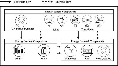
In the effort to address global warming and the energy crisis, manufacturing facilities need to take on a heightened level of accountability by embracing renewable energy sources (RESs). At present, the manufacturing sector is responsible for 21% of the world's 58-gigaton CO2 emissions, further emphasising the urgency of achieving net-zero emissions by 2050. Forecasts suggest that 90% of power generation should originate from RESs by 2050. As manufacturing plants undergo a transition, there is a compelling drive to adopt on-site RES-driven energy production, advancing toward a state of distributed energy sources to effectively tackle these pressing challenges as suggested by Shi et al. (2022). Figure 1 depicts a standard configuration for a factory integrated with RESs that employs a mix of various energy components for its operations, involving the grid; the traditional power sources such as diesel generator (DG), gas turbine (GT), combined heat and power plant (CHP); RESs especially photovoltaic panel (PV) and wind turbine (WT); energy storage components including battery energy storage system (BESS) and thermal energy storage system (TESS); the demand comes from production activities, technical building services (TBS) and the surplus power sold to grid. The variability in flexibility across these components presents challenges in effectively managing complex energy flows. For instance, photovoltaic (PV) generation is not controllable, grid procurement can be adjusted at any time, and certain production activities are inflexible during a job. This intricate interplay of power flow and differential flexibility poses both challenges and opportunities.

Figure 1. An example of the complex energy flows of a factory integrated with RESs.

A schematic of an energy system with supply, storage, and demand components, indicating electricity and thermal flows.

Energy-aware scheduling was first proposed to manage both production and complex energy flows in manufacturing factories (Bruzzone et al. 2012; Fang and Lin 2013), which is effective for factories integrated with RESs like Figure 1. As summarised by the review papers (Akbar and Irohara 2018; Bänsch et al. 2021; Khaled et al. 2022), energy-aware scheduling research has primarily centred on transforming scheduling into optimisation problems, utilising associated algorithms to derive solutions. The formulation of optimisation problems typically involves case-specific objectives (C.-H. Liu 2016), control variables (Biel et al. 2018), and constraints (Xiong, Xing, and Chen 2013). Nevertheless, significant challenges persist in practical applications, primarily arising from the difficulty of effectively implementing solutions due to the unpredictable nature of renewable energy and uncertainties in production. A solution derived from the formulated optimisation problem may lack robustness in the face of unforeseen events. Ideally, a robust solution capable of promptly adapting to unexpected situations and restoring optimal performance is highly desirable. When real-time measurements are employed to enhance robustness and performance (optimality), it invariably demands solving the optimisation problem multiple times, thereby increasing the computational cost. Moreover, existing results do not fully leverage the flexibility in factories integrated with Renewable Energy Sources (RESs). Although many results are available, a comprehensive design that effectively balances the performance of the integrated system (RES with the production line), robustness against unforeseen uncertainties, and computational efficiency is currently absent.

Therefore, in this work, we aim to balance the scheduling performance, robustness and computational cost, and implement it based on a real factory model with a novel method called hybrid event-triggered scheduling(ETHS), which categorises the flexibility of system components, utilises them in different optimisation problems, and involves a design freedom in a user-defined heuristic method to increase computational efficiency. In our approach, we meticulously define the flexibility of different components, facilitating the proper selection of control elements for various stages. Furthermore, we have developed an event-trigger mechanism, specifically engineered to effectively manage disturbances while ensuring that computational costs remain within a practical range. By presenting results from a real-world case, the study illustrates the efficacy of the proposed ETHS in comparison to various existing methods. Notably, the research extensively examines design flexibility through sensitivity analysis of tuning parameters, showcasing how distinct parameter configurations can impact outcomes. This analysis offers valuable design insights for engineering practitioners.

This paper is organised as follows. Section 2 provides an overview of the components within integrated systems, examines the potential sources of disturbances, and explores the state-of-the-art energy-aware production scheduling methods. Section 3 introduces Event-Triggered Hybrid Scheduling (ETHS), a systematic energy-aware production scheduling method. Section 4 presents a case study conducted in a real manufacturing factory to validate the proposed ETHS. Finally, Section 5 concludes the paper.

2. Literature review

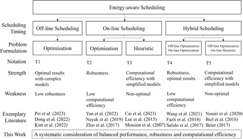
Over the past decades, numerous energy-aware scheduling approaches have been developed to improve scheduling efficiency, particularly in the presence of modelling uncertainties and measurement noises. These approaches can be categorised based on their timing to provide schedules (off-line/on-line/hybrid) or their problem formulation. The problem formulation in this context involves determining how to represent the energy-aware scheduling as specific problem forms for solving. This includes the application of optimisation techniques and heuristic approaches. Optimisation formulations involve creating an objective function and constraints to model the desired outcome or performance criteria, while heuristic techniques leverage practical strategies, rules of thumb, or approximate algorithms to swiftly identify effective solutions, albeit not necessarily optimal. We categorise the existing literature based on the timing of scheduling and the problem formulation as shown in Figure 2, and we list the strengths and weaknesses of different categories that motivate this work.

Figure 2. Classification of current research.

Comparison of off-line, on-line, and hybrid energy-aware scheduling in terms of problem formulation, strengths, weaknesses, and related literature.

Analysing and handling uncertainties or disturbances within factories integrated with RESs has been a central aspect of research in energy-aware scheduling. We categorise the disturbances into energy-related disturbances and production-related disturbances. Energy-related disturbances are usually the difference between the predicted or scheduled energy profile and the measured energy profile. Such a difference is an inevitable source of the disturbance, as mentioned in Kumar and Saravanan (2017). Due to the unpredictable nature of RESs, model-based predictions remain consistently inaccurate, irrespective of the chosen model. Existing models, such as the autoregressive integrated moving average (ARIMA) (Zhai et al. 2017), probability distribution functions (Abikarram and McConky 2017), empirical correlation (Carlucci, Renna, and Materi 2023), and average historical data, all result in non-negligible energy-related disturbances. Additional forms of energy-related disturbances include time-varying rates of energy cost, as documented in Khalaf and Wang (2018), and the adoption of simplified energy models for computational convenience, as emphasised in Li (2015). For example, the commonplace use of average power for machines is highlighted in Khalaf and Wang (2018). Furthermore, in Photovoltaic (PV) models, simplifications often consist of relying exclusively on solar irradiance (Alturki and Awwad 2021), overlooking critical factors such as temperature, which has been demonstrated to play a pivotal role in PV power generation (Chowdhury et al. 2007). Production-related disturbances also influence the efficiency of energy-aware scheduling for the integrated system. Machine breakdown is the most common production-related disturbance, affecting machine availability for an uncertain period. Several models have been developed to characterise these disturbances, including the interval form (Allahverdi and Aydilek 2010), the probabilistic approach (Alfieri 2007), and the language-like fuzzy set (K. Wang, Huang, and Qin 2016). Other production-related disturbances come from production task changes like new job arrivals (Caldeira, Gnanavelbabu, and Vaidyanathan 2020) and job due date change (Eunike et al. 2022). Various approaches have been developed in energy-aware scheduling to enhance robustness with respect to various types of disturbances, as summarised in Figure 2.

The capability to manage these disturbances is influenced by the timing of scheduling, which can be categorised into three distinct types: off-line scheduling, on-line scheduling, and hybrid scheduling. Off-line scheduling has been extensively discussed in the energy-aware scheduling literature, which entails crafting a schedule for a predetermined set of tasks or jobs before their actual execution initiation. It always can be formulated into optimisation problems, for example, in Pei et al. (2023) and Dong and Ye (2022), off-line scheduling was converted into an optimisation problem based on the prediction of renewables using historical data. Over the years, off-line scheduling has evolved along diverse directions. For example, the formulation of cost functions has been discussed as evidenced by both single objective (Khalaf and Wang 2018) and multi-objective perspectives (Karimi and Kwon 2021). New models with extra components such as automated guided vehicles have been proposed, as shown in Cai et al. (2023). Various new algorithms have been developed (G.-S. Liu, Yang, and Cheng 2017) other than standard gradient-descent (Ren, Ye, and Yang 2021). More case studies, such as C.-H. Liu (2016), Kim et al. (2022) have been developed to provide contextualised insights into specific. A distinctive feature of off-line scheduling is its pre-execution occurrence, affording flexibility and accommodating complexity, including intricate characteristics, multi-objective functions, and additional constraints. However, its static nature introduces challenges in responding to unforeseen uncertainties arising from industrial processes, such as machine downtimes or unexpected weather events impacting renewable energy sources like thunderstorms.

When disturbances arise, they directly impact the measurements. Thus, on-line scheduling is utilised during production activities, leveraging real-time measurements for its ability to handle diverse disturbances. Both optimisation techniques and heuristic methods can address these disturbances directly. Heuristic techniques typically provide swift responses with lower computational costs but do not guarantee optimal performance. For example, novel logic-based techniques were used in on-line scheduling to improve the system performance from measurements as discussed in Cai et al. (2023) and Lee and Prabhu (2015). In contrast, optimisation techniques can ensure optimal performance, albeit with high computational costs and potentially slower responses, for example, in Nayak, Lee, and Sutherland (2019) and Yan, Wang, and Wu (2022), it was formulated into an optimisation problem. Disturbance models have already been incorporated into on-line scheduling (Hasan, Sarker, and Essam 2011; K. Wang, Huang, and Qin 2016). To reduce computational cost, techniques such as reducing the frequency of re-scheduling (Zhai et al. 2017) or using simplified models as in Moon and Park (2014) have been used. These techniques are ad hoc. There is no systematic design to balance computational cost, robustness, and optimal performance.

As off-line scheduling occurs before production activities and on-line scheduling takes place during production activities, it is natural to integrate them, resulting in what is commonly referred to as hybrid scheduling. Typically, hybrid scheduling involves two stages: formulating an optimisation problem during the off-line stage and potentially combining it with an optimisation or heuristic approach during the on-line stage as in Beier (2017), Biel et al. (2018), Khalaf and Wang (2018), and Salido et al. (2017). In the on-line stage, efforts have been directed towards handling different types of disturbances using optimisation techniques (Allahverdi and Aydilek 2010) and heuristic techniques (Mouzon, Yildirim, and Twomey 2007; J. Wang et al. 2021). Similar to on-line scheduling, a systematic design to balance computational cost, optimal performance, and robustness to various disturbances is missing. Moreover, existing results do not fully utilise the flexibility in factories integrated with RESs.

It is worthwhile to highlight that another key focus in energy-aware scheduling has consistently been the search for efficient solving algorithms for the formulated optimisation problem. Examples of these algorithms include the iterated greedy algorithm proposed by Katragjini, Vallada, and Ruiz (2013), the genetic algorithm and shifted gap-reduction local search technique introduced by Hasan, Sarker, and Essam (2011), the greedy randomised adaptive search procedure hybridised with an evolutionary local search as presented by Kemmoe, Lamy, and Tchernev (2017), the three-stage decomposition approach outlined in G.-S. Liu, Yang, and Cheng (2017), and the particle swarm optimisation discussed by Nouiri, Bekrar, and Trentesaux (2018). Additionally, widely adopted commercial software, specifically Cplex and Gurobi, has proven popular in solving energy-aware scheduling problems, as demonstrated in Mikhaylidi, Naseraldin, and Yedidsion (2015), Thornton et al. (2017). In our work, we employed Gurobi to address the optimisation problem.

The above literature review presents the state-of-the-art methods employed in energy-aware scheduling. This work concentrates on hybrid scheduling, aiming to offer a systematic design for balancing performance, robustness, and computational cost by exploring the system's flexibility. This is achieved through the careful selection of control components at various stages of hybrid scheduling. Additionally, we introduce an event-trigger mechanism designed to efficiently enhance robustness while maintaining optimal performance and manageable computational costs.

3. Event-triggered hybrid scheduling (ETHS)

Event-triggered hybrid scheduling (ETHS) is a comprehensive methodology that integrates three distinct optimisation problems and a decision module to efficiently initialise and update schedules for different types of components based on their flexibility within the integrated system. In this section, we focus on formulating the three different optimisation problems, the real-time decision module and the flexibility-based categorisation criteria for components. The hybrid nature of ETHS combines both off-line scheduling and on-line scheduling. Initially, an off-line schedule is calculated before the production starts. Then, depending on the performance evaluation or predicted performance, either on-line adjustment is triggered for highly flexible components or on-line rescheduling is triggered for all manipulable components. This hybrid approach fully explores the flexibility in the integrated system, enhances the system's robustness in dealing with disturbances, and simultaneously reduces the computational cost.

This section starts by categorising the components and formulating the problem, followed by the introduction of three optimisation problems: off-line scheduling, on-line adjustment, and on-line rescheduling. Additionally, an event-trigger mechanism is presented as part of the scheduling process.

3.1. Categorisation of components

With the aim of effectively utilising the varying flexibility of heterogeneous components, the first step of ETHS is to categorise the components of a given integrated system based on their individual levels of flexibility. Consequently, we define three categories to capture the varying levels of flexibility among the components based on the performance evaluation:

• Non-dispatchable components refer to those in which their information at any sampling instant can be measured, but cannot be manipulated. For example, a photovoltaic (PV) system can be usually defined as a non-dispatchable component, its electricity generation can only be measured.

• Fully-dispatchable components have high flexibility, in which their information at any sampling instant can be both measured and manipulated. For example, if a battery energy storage system (ESS) is defined as a fully-dispatchable component, it means the charging power or discharging power can be manipulated at any sampling instant of ESS.

• Partially-dispatchable components have low flexibility, which can be rescheduled under specific conditions or criteria. In the context of the proposed ETHS methodology, these components can have their information manipulated only when the system performance is assessed as unsatisfactory. For example, if the production line is classified as a partially-dispatchable component, the production schedules will not be rescheduled unless the system finds that the production task may not be finished in time. The detailed evaluation of system performance is case-dependent. It will be discussed in Section 3.4 S3.

Although the categorisation of components may vary depending on the specific case, there are a few general principles that can guide the process. Firstly, categorisation is based on the knowledge of the integrated system and typically occurs prior to the scheduling phase. This means that the categorisation takes into account the characteristics and behaviour of the components in the system, such as their operational constraints, flexibility, and availability. For example, a photovoltaic (PV) system is typically categorised as non-dispatchable, which is derived from the understanding of its inherent characteristics and limitations.

Secondly, the categorisation of components is often related to specific costs and risks identified within the integrated system. Operators or decision-makers consider the potential costs and risks associated with different components and their scheduling options. For instance, if operators anticipate that frequent rescheduling of a production line will lead to operational chaos or increased risks, they may categorise it as a partially-dispatchable component. On the other hand, if they believe that frequent rescheduling will result in higher benefits with minimal risks, they may categorise the production line as fully-dispatchable.

3.2. Problem formulation

This subsection provides an introduction to the definitions of various variables used in ETHS. These variables play a crucial role in formulating the three optimisation problems accurately within the methodology.

Definition 3.1

Measured State Variable

In the context of ETHS, measured state variables represent the quantitative operational status of components in the factory that can be measured using sensors, and we use a vector $\overrightarrow{\mathbf{x}}\left[k\right]$ to represent the state variables of all components at kth time step. According to our categorisation of components, the state variables $\overrightarrow{\mathbf{x}}\left[k\right]$ can be further classified into non-dispatchable states, partially-dispatchable states and fully-dispatchable states, as is shown in (1(1) $\overrightarrow{\mathbf{x}}\left[k\right]={\left[\begin{array}{c}{\mathbf{x}}_{\mathrm{ND}}^T\left[k\right],{\mathbf{x}}_{\mathrm{FD}}^T\left[k\right],{\mathbf{x}}_{\mathrm{PD}}^T\left[k\right]\end{array}\right]}^T.$(1) ). (1) $\overrightarrow{\mathbf{x}}\left[k\right]={\left[\begin{array}{c}{\mathbf{x}}_{\mathrm{ND}}^T\left[k\right],{\mathbf{x}}_{\mathrm{FD}}^T\left[k\right],{\mathbf{x}}_{\mathrm{PD}}^T\left[k\right]\end{array}\right]}^T.$(1) In ETHS, one component can include several state variables. For example, the component ESS includes the state variable of charging power and state of charge.

Definition 3.2

Predicted/scheduled State Variable at kth step

In this work, $\overrightarrow{\hat{\mathbf{x}}}[k+i|k]$ is the predicted state using the model and the current measurement $\overrightarrow{\mathbf{x}}\left[k\right]$ to compute future ith step. For example, $\overrightarrow{\hat{\mathbf{x}}}\left[10|5\right]$ means the predicted state at 10th time step, where the prediction occurs at the 5th time step.

Definition 3.3

Constraint

In the context of ETHS, models of components appear in the scheduling problem in the form of constraints. For example, there may be a power limit for ESS charging, or there may be an energy balance constraint between demand and supply, these equations and inequalities will become constraints. Moreover, regression models such as ARIMA or dynamic models characterised by different equations can be also treated as constraints in the scheduling or optimisation.

Definition 3.4

Objective Function

The objective function $J[k+N|k]$ is the quantitative scheduling target at the kth sampling predicted to $(k+N)$th step where N is an integer indicating the prediction horizon as is shown in (2(2) $\underset{\overrightarrow{\mathit{\xi }}\left[k\right]}{min}J[k+N|k]=\underset{\overrightarrow{\mathit{\xi }}\left[k\right]}{min}\sum _{i=0}^N\mathbf{l}[k+i|k],$(2) )–(3(3) $\mathbf{l}[k+i|k]=\mathbf{l}\left(\overrightarrow{\hat{\mathbf{x}}}\right[k+i|k],\overrightarrow{\mathit{\theta }}),$(3) ). (2) $\underset{\overrightarrow{\mathit{\xi }}\left[k\right]}{min}J[k+N|k]=\underset{\overrightarrow{\mathit{\xi }}\left[k\right]}{min}\sum _{i=0}^N\mathbf{l}[k+i|k],$(2) where (3) $\mathbf{l}[k+i|k]=\mathbf{l}\left(\overrightarrow{\hat{\mathbf{x}}}\right[k+i|k],\overrightarrow{\mathit{\theta }}),$(3) where $\overrightarrow{\hat{\mathbf{x}}}[k+i|k]$ is the predicted state. The value of N can be 0, meaning scheduling on a specific time step, or can be larger than 0, meaning scheduling over the time period N. At the kth instant, the cost $\mathbf{l}\left[k\right]$ consists of the states $\overrightarrow{\mathbf{x}}\left[k\right]$ and some constant parameters $\overrightarrow{\mathit{\theta }}$ such as weighting among different states. Here $\overrightarrow{\mathit{\xi }}\left[k\right]$ is the control variable for the optimisation at the kth sampling instant. It consists of a future predicted state, which can be either fully dispatchable or partially dispatchable if on-line adjustment is triggered. For example, it can include ${\overrightarrow{\hat{\mathbf{x}}}}_{\mathrm{FD}}[k+1|k]$ and ${\overrightarrow{\hat{\mathbf{x}}}}_{\mathrm{FD}}[k+2|k]$ when N = 2. More details will be provided in Section 3.3.

One important aspect of ETHS is the objective function, which represents the cost at a specific time step $\mathbf{l}\left[k\right]$ and is accumulated over a predicted period of time.

3.3. Framework of ETHS

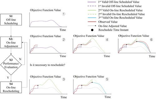
The framework of ETHS encompasses three distinct scheduling problems and a decision module, which are organised into four sequential steps denoted as S1 to S4. These steps form a comprehensive flowchart that outlines the process of constructing the ETHS framework.

S1:	Off-line scheduling. The primary objective of Step S1 in the ETHS framework is to initialise the schedules for the integrated system. In this step, the objective function of S1 is focussed on optimising the overall system performance, which may involve minimising energy costs or reducing makespan, among other performance criteria. Controlled variables are fully-dispatchable and partially-dispatchable components. Such an off-line appeared in literature, for example, Khalaf and Wang (2018) used the day-ahead predicted PV generation state to calculate the optimal states for production, ESS and grid procurement, which is off-line scheduling. Similarly, Zhai et al. (2017) used predicted wind generation state to provide schedules for production and grid procurement.
S2:	On-line adjustment. The purpose of S2 is to handle disturbances when it's unnecessary to reschedule partially-dispatchable components, so the objective function of S2 is to minimise the gap between two objective function values where one using measured state variables to calculate and the other using predicted state variables to calculate, by re-adjusting fully dispatchable component. Thus, the controlled components are fully-dispatchable components. S2 is based on the assumption that the previously calculated objective function value is an optimal solution and fully-dispatchable components can be used to approach it to handle the disturbances without the need for re-scheduling using both fully-dispatchable components and partially-dispatchable components.
S3:	Performance evaluation. S3 is implemented to judge whether it is necessary to reschedule the partially-dispatchable components. In S3, real-timely measured and real-timely predicted states for all components can be used to compose a function $\mathbf{J}\left[k\right]$ at kth sampling instant. Meanwhile, a parameter ε should be decided as the rescheduling threshold, only when $\mathbf{J}\left[k\right]\ge ϵ$ will the rescheduling be triggered. In literature, such an evaluation exists, for example, Sang, Tan, and Liu (2021) defined the predicted job delay time ratio as the cost function and set the threshold as $20\mathrm{\%}$, which means if the predicted job delay is more than $20\mathrm{\%}$ will the production rescheduling be triggered. Another research by Eunike et al. (2022) considered deadline change and production disturbances to trigger rescheduling. In this paper, the idea is extended that all partially-dispatchable components will be rescheduled when the cost function is greater than the threshold. To point out, the threshold can be determined as a tunable parameter to dynamically control the rescheduling frequency.
S4:	On-line rescheduling. The purpose of S4 is to reschedule partially-dispatchable components when the system doesn't work well. The objective function of S4 is the system performance again, which is the same as S1. The controlled components are partially-dispatchable components and fully-dispatchable components, and the scheduling horizon is the reminder of the entire horizon. S4 will only be triggered when S3 judges that the system doesn't work well and rescheduling is needed.
Loop:	For each time step, if S3 judges that the rescheduling is not needed at the kth sampling instant, S4 will not be implemented, and S2 will be implemented again at the next time step k + 1. If S3 judges that the system doesn't work well, S4 will be triggered, providing re-scheduling. This process will be repeated from S2, S3, to S4 at next step k + 1.

An illustrative example is presented in Figure 3 to showcase the application of the ETHS framework. At the beginning in 1 ⃝, S1 provides off-line schedules for partially-dispatchable and fully-dispatchable components, at the same time, a sequence of future desired operation are obtained. Subsequently in 2 ⃝, S2 identifies the difference between the two objective function values calculated through measured and predicted states and minimises the mismatch by tuning the fully-dispatchable components. S2 will run at each time step until at a specific time, S3 verifies that the performance of the integrated system is not satisfying, it will trigger S4 3 ⃝ to update the schedules for partially-dispatchable components and fully-dispatchable components by doing re-scheduling, leading to a new sequence of future desired operations. This process will be repeated.

Figure 3. Framework and example of ETHS.

A diagram of ETHS with a scheduling process flowchart and graphs showing objective function values over time for scheduling decisions.

In summary, the ETHS framework consists of four sequential steps: S1 for initialising schedules, S2 for handling disturbances by leveraging the flexibility of fully-dispatchable components, S3 for evaluating the current system performance and determining the need for rescheduling, and S4 for performing rescheduling if the current performance is unsatisfactory.

By incorporating these steps, ETHS addresses the gap identified in the literature and provides a systematic approach to balance the robustness and computational cost by exploring the flexibility in energy-aware production scheduling in integrated systems. To validate the effectiveness of ETHS, a case study based on a real manufacturing industry will be conducted, further demonstrating the practical applicability and benefits of the proposed framework.

4. Case study: metal production factory

A case study of a metal production factory will be used to validate the proposed ETHS in a factory. In Section 4.1, we will provide a comprehensive description of the integrated system. Section 4.2 will illustrate the practical implementation of ETHS within the described system, which will serve as a baseline when comparisons are needed. While heuristic adjustments are prevalent in the literature, our primary focus is on achieving a balance between optimal performance, robustness, and computational cost. In our case study, both off-line and on-line scheduling are reformulated into corresponding optimisation problems, and all problems are solved using Gurobi. Section 4.3 compares ETHS with traditional methods. Section 4.4 validates the sensitivity of each step from S2 to S4. Subsequently, Section 4.5 discusses how different categorisations will affect the performance of ETHS. Section 4.6 shows how different event-trigger conditions will affect the performance of ETHS.

4.1. System description

The metal production factory is operated with the objective of minimising energy costs at the same time as finishing the production task, which consists of the following components: PV, GaT, ESS, grid, and a 5-machine production line, whose energy flow can be found in Figure 4.

Figure 4. System components and energy flow of the factory.

Diagram showing energy and material flow among photovoltaic (PV), energy storage system (ESS), grid, gas turbine (GaT) and a production line of 5 machines.

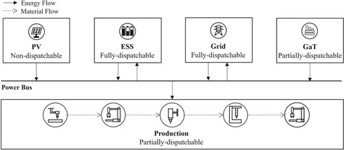
In the given setting, the objective is to complete a total of 50 products by the end of the day. The production process involves five machines, namely the turret punch, brake press, welding bay, angle grinder, and powder coating machine. Each machine represents a specific step in the production process. The products must follow a predetermined sequence, starting from the first machine and progressing through each subsequent machine until reaching the final machine. This sequential order adheres to the flow shop model, where the products flow through the machines in a fixed sequence

The stochastic factor in the case study comes from random production disturbances which follow an exponential distribution, thus all the scheduling experiments are repeated 3 times, and the results are the average result of the 3 experiments.

4.2. Scenario 0: a baseline ETHS

The categorisation is as follows: PV and grid are non-dispatchable components, ESS is a fully-dispatchable component, GaT and production line are partially-dispatchable components, and their states and parameters can be found in Tables 1 and 2. Notably, the exponential distributions of random production disturbance are expressed in (4(4) $\{\begin{array}{l}P\left({\hat{\mathbf{x}}}_{2,i}\right[k]=0|{\mathbf{x}}_{2,i}[k]=1)=1-e^{-{\theta }_{12}{T}_{\mathrm{on}}}\\ P\left({\hat{\mathbf{x}}}_{2,i}\right[k+1]=1|{\hat{\mathbf{x}}}_{2,i}[k]=0)=1-e^{-{\theta }_{13}{T}_{\mathrm{bd}}}\end{array},$(4) ), including disturbance time step and breakdown time, where $T_{\mathrm{on}}$ means the time that the machine has operated normally since the last recovery from disturbance, and $T_{\mathrm{bd}}$ means the time that the machine has been under disturbance. (4) $\{\begin{array}{l}P\left({\hat{\mathbf{x}}}_{2,i}\right[k]=0|{\mathbf{x}}_{2,i}[k]=1)=1-e^{-{\theta }_{12}{T}_{\mathrm{on}}}\\ P\left({\hat{\mathbf{x}}}_{2,i}\right[k+1]=1|{\hat{\mathbf{x}}}_{2,i}[k]=0)=1-e^{-{\theta }_{13}{T}_{\mathrm{bd}}}\end{array},$(4)

Table 1. States variables for the metal production factory.

States	Description
States in ND Components
$x_1\in {\mathcal{R}}^1$	Power of PV generation
States in PD Components
${\mathbf{x}}_2\in {\mathcal{R}}^{10}$	Machine status on or off for each machine
${\mathbf{x}}_3\in {\mathcal{R}}^{10}$	Operation status starts or not start on each machine
${\mathbf{x}}_4\in {\mathcal{R}}^{10}$	Number of operations finished on each machine
$x_5\in {\mathcal{R}}^1$	GaT generation power
States in FD Components
$x_6\in {\mathcal{R}}^1$	ESS charging power
$x_7\in {\mathcal{R}}^1$	ESS discharging power
$x_8\in {\mathcal{R}}^1$	ESS state of charge (SOC)
$x_9\in {\mathcal{R}}^1$	Grid electricity procurement power
$x_{10}\in {\mathcal{R}}^1$	Grid electricity feed-in power

Table 2. Parameters for the metal production factory.

Parameter	Description	Value
${\mathit{\theta }}_1\in {\mathcal{R}}^4$	Machine power for 5 machines (kW)	[25.8,0.66,0.65,1.69,35.8]
${\mathit{\theta }}_2\in {\mathcal{R}}^4$	Operation time for 5 operations (5 min)	[3,2,3,1,2]
${\theta }_3\in {\mathcal{R}}^1$	Gas price ($)	1.83
${\theta }_4\in {\mathcal{R}}^1$	ESS charging/discharging efficiency	0.9
${\theta }_5\in {\mathcal{R}}^1$	ESS fixed operational cost ($/5 min)	0.003
${\theta }_6\in {\mathcal{R}}^1$	ESS charging/discharging degradation cost ($/kWh)	0.0006
${\theta }_7\in {\mathcal{R}}^1$	ESS maximum capacity (kWh)	50
${\theta }_8\in {\mathcal{R}}^1$	ESS depth of discharge	80%
${\theta }_9\in {\mathcal{R}}^1$	ESS maximum charging/ discharging power (kW)	50
${\mathit{\theta }}_{10}\in {\mathcal{R}}^{288}$	Grid electricity procurement price ($/kWh)	0.330 from 9am to 9pm 0.187 from 9pm to 9am
${\theta }_{11}\in {\mathcal{R}}^1$	Grid electricity feed-in tariff ($/kWh)	0.052
${\theta }_{12}\in {\mathcal{R}}^1$	Production disturbance possibility parameter	0.1
${\theta }_{13}\in {\mathcal{R}}^1$	Production disturbance time parameter	2
${\theta }_{14}\in {\mathcal{R}}^1$	Number of production task	50

Firstly, S1 is implemented, which provides a day-ahead schedule for machine status, GaT electricity generation, ESS charging power and grid procurement plan. The objective function and constraints can be found in (5(5) $\begin{array}{rl}{\mathbf{l}}_{1,0}& ={\hat{\mathbf{x}}}_9\left[i|0\right]\cdot {\mathit{\theta }}_{10,0}-{\hat{\mathbf{x}}}_9\left[i|0\right]\cdot {\theta }_{11}+{\theta }_5\\ & +\left({\hat{\mathbf{x}}}_6\right[i|0]+{\hat{\mathbf{x}}}_7[i|0\left]\right)\cdot {\theta }_4+{\hat{\mathbf{x}}}_5\left[i|0\right]\cdot {\theta }_3\end{array}$(5) )–(9(9) $\begin{array}{rl}{\hat{\mathbf{x}}}_{4,m}\left[i|0\right]& \ge {\hat{\mathbf{x}}}_{4,m+1}\left[i|0\right]+{\hat{\mathbf{x}}}_{2,m+1}\left[i|0\right],\\ & i=1,2,\dots ,288.\end{array}$(9) ). Since it's off-line, all the prediction occurs at 0th time step. ${\mathbf{l}}_{1,0}$ means S1 occurs at 0th time step in (5(5) $\begin{array}{rl}{\mathbf{l}}_{1,0}& ={\hat{\mathbf{x}}}_9\left[i|0\right]\cdot {\mathit{\theta }}_{10,0}-{\hat{\mathbf{x}}}_9\left[i|0\right]\cdot {\theta }_{11}+{\theta }_5\\ & +\left({\hat{\mathbf{x}}}_6\right[i|0]+{\hat{\mathbf{x}}}_7[i|0\left]\right)\cdot {\theta }_4+{\hat{\mathbf{x}}}_5\left[i|0\right]\cdot {\theta }_3\end{array}$(5) ), ESS charging limit, ESS state model, gas turbine generation limit and energy balance model are in (6(6) $\{\begin{array}{l}{\hat{\mathbf{x}}}_6\left[i|0\right]\le {\theta }_9\\ {\hat{\mathbf{x}}}_7\left[i|0\right]\le {\theta }_9\\ {\hat{\mathbf{x}}}_8\left[i|0\right]\ge {\theta }_7\cdot (1-{\theta }_8)/2\\ {\hat{\mathbf{x}}}_8\left[i|0\right]\le {\theta }_7\cdot (1+{\theta }_8)/2\\ {\hat{\mathbf{x}}}_8[i+1|0]\\ ={\hat{\mathbf{x}}}_8\left[i|0\right]+{\theta }_4\cdot {\hat{\mathbf{x}}}_6\left[i|0\right]-1/{\theta }_4\cdot {\hat{\mathbf{x}}}_7\left[i|0\right]\\ {\hat{\mathbf{x}}}_1\left[i|0\right]+{\hat{\mathbf{x}}}_9\left[i|0\right]+{\hat{\mathbf{x}}}_7\left[i|0\right]+{\hat{\mathbf{x}}}_5\left[i|0\right]\\ ={\displaystyle \sum _{m=1}^5{\hat{\mathbf{x}}}_{2,m}\left[i|0\right]\cdot {\mathit{\theta }}_{1,m}+{\hat{\mathbf{x}}}_5\left[i|0\right]+{\hat{\mathbf{x}}}_7\left[i|0\right]}\end{array}$(6) ), ESS initial and end state, production task completion constraint are in (7(7) $\{\begin{array}{l}{\hat{\mathbf{x}}}_8\left[0|0\right]={\theta }_7\cdot 0.5\\ {\hat{\mathbf{x}}}_8\left[288|0\right]={\theta }_7\cdot 0.5\\ {\hat{\mathbf{x}}}_{4,5}\left[288|0\right]\ge {\theta }_{14}\end{array}$(7) ), 5-machine production model is in (8(8) $\{\begin{array}{ll}{\hat{\mathbf{x}}}_{4,m}\left[i|0\right]=0,& i=1,2,\dots ,{\mathit{\theta }}_{2,m}.\\ {\hat{\mathbf{x}}}_{4,m}\left[i|0\right]={\displaystyle \sum _{j=i}^{i-{\theta }_{2,m}}{\hat{\mathbf{x}}}_{3,m}\left[j|0\right],}& i={\mathit{\theta }}_{2,m},\dots ,288\\ {\hat{\mathbf{x}}}_{2,m}\left[i|0\right]={\displaystyle \sum _{j=0}^i{\hat{\mathbf{x}}}_{3,m}\left[j|0\right],}& i=1,2,\dots ,{\mathit{\theta }}_{2,m}\\ {\hat{\mathbf{x}}}_{2,m}[i-1|0]& \\ ={\displaystyle \sum _{j=i-{\theta }_{2,m}}^i{\hat{\mathbf{x}}}_{3,m}\left[j|0\right],}& i={\mathit{\theta }}_{2,m},\dots ,288\\ {\hat{\mathbf{x}}}_{3,m}\left[i|0\right]\cdot {\mathit{\theta }}_{2,m}& \\ \le {\displaystyle \sum _{j=0}^{i+{\theta }_{2,m}}{\hat{\mathbf{x}}}_{2,m}\left[j|0\right],}& i=1,2,\dots ,\\ & 288-{\mathit{\theta }}_{2,m}\end{array}$(8) )–(9(9) $\begin{array}{rl}{\hat{\mathbf{x}}}_{4,m}\left[i|0\right]& \ge {\hat{\mathbf{x}}}_{4,m+1}\left[i|0\right]+{\hat{\mathbf{x}}}_{2,m+1}\left[i|0\right],\\ & i=1,2,\dots ,288.\end{array}$(9) ).

The objective function (5(5) $\begin{array}{rl}{\mathbf{l}}_{1,0}& ={\hat{\mathbf{x}}}_9\left[i|0\right]\cdot {\mathit{\theta }}_{10,0}-{\hat{\mathbf{x}}}_9\left[i|0\right]\cdot {\theta }_{11}+{\theta }_5\\ & +\left({\hat{\mathbf{x}}}_6\right[i|0]+{\hat{\mathbf{x}}}_7[i|0\left]\right)\cdot {\theta }_4+{\hat{\mathbf{x}}}_5\left[i|0\right]\cdot {\theta }_3\end{array}$(5) ) is the overall energy cost, including grid purchase cost, grid feed-in tariff, ESS usage cost and GaT generation cost. (5) $\begin{array}{rl}{\mathbf{l}}_{1,0}& ={\hat{\mathbf{x}}}_9\left[i|0\right]\cdot {\mathit{\theta }}_{10,0}-{\hat{\mathbf{x}}}_9\left[i|0\right]\cdot {\theta }_{11}+{\theta }_5\\ & +\left({\hat{\mathbf{x}}}_6\right[i|0]+{\hat{\mathbf{x}}}_7[i|0\left]\right)\cdot {\theta }_4+{\hat{\mathbf{x}}}_5\left[i|0\right]\cdot {\theta }_3\end{array}$(5) Constraints in (6(6) $\{\begin{array}{l}{\hat{\mathbf{x}}}_6\left[i|0\right]\le {\theta }_9\\ {\hat{\mathbf{x}}}_7\left[i|0\right]\le {\theta }_9\\ {\hat{\mathbf{x}}}_8\left[i|0\right]\ge {\theta }_7\cdot (1-{\theta }_8)/2\\ {\hat{\mathbf{x}}}_8\left[i|0\right]\le {\theta }_7\cdot (1+{\theta }_8)/2\\ {\hat{\mathbf{x}}}_8[i+1|0]\\ ={\hat{\mathbf{x}}}_8\left[i|0\right]+{\theta }_4\cdot {\hat{\mathbf{x}}}_6\left[i|0\right]-1/{\theta }_4\cdot {\hat{\mathbf{x}}}_7\left[i|0\right]\\ {\hat{\mathbf{x}}}_1\left[i|0\right]+{\hat{\mathbf{x}}}_9\left[i|0\right]+{\hat{\mathbf{x}}}_7\left[i|0\right]+{\hat{\mathbf{x}}}_5\left[i|0\right]\\ ={\displaystyle \sum _{m=1}^5{\hat{\mathbf{x}}}_{2,m}\left[i|0\right]\cdot {\mathit{\theta }}_{1,m}+{\hat{\mathbf{x}}}_5\left[i|0\right]+{\hat{\mathbf{x}}}_7\left[i|0\right]}\end{array}$(6) ) are energy constraints, including ESS power limit, GaT power limit, ESS state equation, and energy balance equations. For any $i=1,2,\dots ,288$: (6) $\{\begin{array}{l}{\hat{\mathbf{x}}}_6\left[i|0\right]\le {\theta }_9\\ {\hat{\mathbf{x}}}_7\left[i|0\right]\le {\theta }_9\\ {\hat{\mathbf{x}}}_8\left[i|0\right]\ge {\theta }_7\cdot (1-{\theta }_8)/2\\ {\hat{\mathbf{x}}}_8\left[i|0\right]\le {\theta }_7\cdot (1+{\theta }_8)/2\\ {\hat{\mathbf{x}}}_8[i+1|0]\\ ={\hat{\mathbf{x}}}_8\left[i|0\right]+{\theta }_4\cdot {\hat{\mathbf{x}}}_6\left[i|0\right]-1/{\theta }_4\cdot {\hat{\mathbf{x}}}_7\left[i|0\right]\\ {\hat{\mathbf{x}}}_1\left[i|0\right]+{\hat{\mathbf{x}}}_9\left[i|0\right]+{\hat{\mathbf{x}}}_7\left[i|0\right]+{\hat{\mathbf{x}}}_5\left[i|0\right]\\ ={\displaystyle \sum _{m=1}^5{\hat{\mathbf{x}}}_{2,m}\left[i|0\right]\cdot {\mathit{\theta }}_{1,m}+{\hat{\mathbf{x}}}_5\left[i|0\right]+{\hat{\mathbf{x}}}_7\left[i|0\right]}\end{array}$(6) Constraints in (7(7) $\{\begin{array}{l}{\hat{\mathbf{x}}}_8\left[0|0\right]={\theta }_7\cdot 0.5\\ {\hat{\mathbf{x}}}_8\left[288|0\right]={\theta }_7\cdot 0.5\\ {\hat{\mathbf{x}}}_{4,5}\left[288|0\right]\ge {\theta }_{14}\end{array}$(7) ) define all the initial values and final values, including ESS initial and final state of charge, and production task completion. (7) $\{\begin{array}{l}{\hat{\mathbf{x}}}_8\left[0|0\right]={\theta }_7\cdot 0.5\\ {\hat{\mathbf{x}}}_8\left[288|0\right]={\theta }_7\cdot 0.5\\ {\hat{\mathbf{x}}}_{4,5}\left[288|0\right]\ge {\theta }_{14}\end{array}$(7) For $m=1,\dots ,5$. Constraints in (8(8) $\{\begin{array}{ll}{\hat{\mathbf{x}}}_{4,m}\left[i|0\right]=0,& i=1,2,\dots ,{\mathit{\theta }}_{2,m}.\\ {\hat{\mathbf{x}}}_{4,m}\left[i|0\right]={\displaystyle \sum _{j=i}^{i-{\theta }_{2,m}}{\hat{\mathbf{x}}}_{3,m}\left[j|0\right],}& i={\mathit{\theta }}_{2,m},\dots ,288\\ {\hat{\mathbf{x}}}_{2,m}\left[i|0\right]={\displaystyle \sum _{j=0}^i{\hat{\mathbf{x}}}_{3,m}\left[j|0\right],}& i=1,2,\dots ,{\mathit{\theta }}_{2,m}\\ {\hat{\mathbf{x}}}_{2,m}[i-1|0]& \\ ={\displaystyle \sum _{j=i-{\theta }_{2,m}}^i{\hat{\mathbf{x}}}_{3,m}\left[j|0\right],}& i={\mathit{\theta }}_{2,m},\dots ,288\\ {\hat{\mathbf{x}}}_{3,m}\left[i|0\right]\cdot {\mathit{\theta }}_{2,m}& \\ \le {\displaystyle \sum _{j=0}^{i+{\theta }_{2,m}}{\hat{\mathbf{x}}}_{2,m}\left[j|0\right],}& i=1,2,\dots ,\\ & 288-{\mathit{\theta }}_{2,m}\end{array}$(8) ) are the constraints for each machine, including the initial states, machine job finished number calculation, and uninterruptible jobs. (8) $\{\begin{array}{ll}{\hat{\mathbf{x}}}_{4,m}\left[i|0\right]=0,& i=1,2,\dots ,{\mathit{\theta }}_{2,m}.\\ {\hat{\mathbf{x}}}_{4,m}\left[i|0\right]={\displaystyle \sum _{j=i}^{i-{\theta }_{2,m}}{\hat{\mathbf{x}}}_{3,m}\left[j|0\right],}& i={\mathit{\theta }}_{2,m},\dots ,288\\ {\hat{\mathbf{x}}}_{2,m}\left[i|0\right]={\displaystyle \sum _{j=0}^i{\hat{\mathbf{x}}}_{3,m}\left[j|0\right],}& i=1,2,\dots ,{\mathit{\theta }}_{2,m}\\ {\hat{\mathbf{x}}}_{2,m}[i-1|0]& \\ ={\displaystyle \sum _{j=i-{\theta }_{2,m}}^i{\hat{\mathbf{x}}}_{3,m}\left[j|0\right],}& i={\mathit{\theta }}_{2,m},\dots ,288\\ {\hat{\mathbf{x}}}_{3,m}\left[i|0\right]\cdot {\mathit{\theta }}_{2,m}& \\ \le {\displaystyle \sum _{j=0}^{i+{\theta }_{2,m}}{\hat{\mathbf{x}}}_{2,m}\left[j|0\right],}& i=1,2,\dots ,\\ & 288-{\mathit{\theta }}_{2,m}\end{array}$(8) Constraints in (9(9) $\begin{array}{rl}{\hat{\mathbf{x}}}_{4,m}\left[i|0\right]& \ge {\hat{\mathbf{x}}}_{4,m+1}\left[i|0\right]+{\hat{\mathbf{x}}}_{2,m+1}\left[i|0\right],\\ & i=1,2,\dots ,288.\end{array}$(9) ) are the relationship among machines, which means a machine can only start processing when the previous job is finished For $m=1,\dots ,4$ (9) $\begin{array}{rl}{\hat{\mathbf{x}}}_{4,m}\left[i|0\right]& \ge {\hat{\mathbf{x}}}_{4,m+1}\left[i|0\right]+{\hat{\mathbf{x}}}_{2,m+1}\left[i|0\right],\\ & i=1,2,\dots ,288.\end{array}$(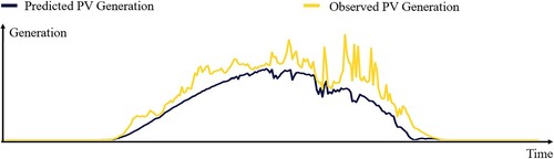9) Real-time disturbances are unavoidable after S1. In accordance with the review of disturbances in Section 2.2, we apply PV prediction error as the energy-related disturbances and involve machine breakdown, job time change, and other disturbances in a general disturbance, which follows an exponential distribution (Xiong, Xing, and Chen 2013), which has parameter ${\theta }_{11}$ and ${\theta }_{12}$ in Table 2. To visually show the real-time disturbances, we provide the Gantt chart of production under random production disturbances, and the difference between PV generation prediction and observation, which are shown in Figures 5 and 6.

Secondly, S2 is implemented to minimise the gap between the predicted objective function value and the measured objective function value by controlling ESS. The scheduling problem of S2 is listed below from (10(10) $\begin{array}{rl}{\mathbf{l}}_{2,k}& =|{\mathbf{l}}_1\left({\overrightarrow{\mathbf{x}}}_{\mathrm{ND}}\right[k],{\overrightarrow{\mathbf{x}}}_{\mathrm{PD}}[k],{\overrightarrow{\mathbf{x}}}_{\mathrm{FD}}[k|k],\overrightarrow{\mathit{\theta }})\\ & -{\mathbf{l}}_1\left(\overrightarrow{\mathbf{x}}\right[k|k_{\mathrm{last}}],\overrightarrow{\mathit{\theta }})|.\end{array}$(10) )–(11(11) $\{\begin{array}{l}{\hat{\mathbf{x}}}_6\left[k|k\right]\le {\theta }_9\\ {\hat{\mathbf{x}}}_7\left[k|k\right]\le {\theta }_9\\ {\hat{\mathbf{x}}}_8\left[k|k\right]\ge {\theta }_7\cdot (1-{\theta }_8)/2\\ {\hat{\mathbf{x}}}_8\left[k|k\right]\le {\theta }_7\cdot (1+{\theta }_8)/2\\ {\hat{\mathbf{x}}}_8\left[k|k\right]={\hat{\mathbf{x}}}_8\left[k|k\right]+{\theta }_4\cdot {\hat{\mathbf{x}}}_6\left[k|k\right]\\ -1/{\theta }_4\cdot {\hat{\mathbf{x}}}_7\left[k|k\right]\\ {\hat{\mathbf{x}}}_1\left[k\right]+{\hat{\mathbf{x}}}_9\left[k|k\right]+{\hat{\mathbf{x}}}_7\left[k|k\right]+{\hat{\mathbf{x}}}_5\left[k\right]\\ ={\displaystyle \sum _{m=1}^5{\hat{\mathbf{x}}}_{2,m}\left[k\right]\cdot {\mathit{\theta }}_{1,m}+{\hat{\mathbf{x}}}_5\left[k\right]+{\hat{\mathbf{x}}}_7\left[k|k\right]}\end{array}$(11) ). ${\mathbf{l}}_{2,k}$ means S2 occurs at kth time step in (10(10) $\begin{array}{rl}{\mathbf{l}}_{2,k}& =|{\mathbf{l}}_1\left({\overrightarrow{\mathbf{x}}}_{\mathrm{ND}}\right[k],{\overrightarrow{\mathbf{x}}}_{\mathrm{PD}}[k],{\overrightarrow{\mathbf{x}}}_{\mathrm{FD}}[k|k],\overrightarrow{\mathit{\theta }})\\ & -{\mathbf{l}}_1\left(\overrightarrow{\mathbf{x}}\right[k|k_{\mathrm{last}}],\overrightarrow{\mathit{\theta }})|.\end{array}$(10) ). To explain the objective function, it's the absolute difference between two objective functions, one is calculated by the measured ND and PD state and the control variable of FD state at kth time step; the other objective function is calculated by the predicted states in the previous schedule where we use $k_{\mathrm{last}}$ to denote. (10) $\begin{array}{rl}{\mathbf{l}}_{2,k}& =|{\mathbf{l}}_1\left({\overrightarrow{\mathbf{x}}}_{\mathrm{ND}}\right[k],{\overrightarrow{\mathbf{x}}}_{\mathrm{PD}}[k],{\overrightarrow{\mathbf{x}}}_{\mathrm{FD}}[k|k],\overrightarrow{\mathit{\theta }})\\ & -{\mathbf{l}}_1\left(\overrightarrow{\mathbf{x}}\right[k|k_{\mathrm{last}}],\overrightarrow{\mathit{\theta }})|.\end{array}$(10) Constraints in (11(11) $\{\begin{array}{l}{\hat{\mathbf{x}}}_6\left[k|k\right]\le {\theta }_9\\ {\hat{\mathbf{x}}}_7\left[k|k\right]\le {\theta }_9\\ {\hat{\mathbf{x}}}_8\left[k|k\right]\ge {\theta }_7\cdot (1-{\theta }_8)/2\\ {\hat{\mathbf{x}}}_8\left[k|k\right]\le {\theta }_7\cdot (1+{\theta }_8)/2\\ {\hat{\mathbf{x}}}_8\left[k|k\right]={\hat{\mathbf{x}}}_8\left[k|k\right]+{\theta }_4\cdot {\hat{\mathbf{x}}}_6\left[k|k\right]\\ -1/{\theta }_4\cdot {\hat{\mathbf{x}}}_7\left[k|k\right]\\ {\hat{\mathbf{x}}}_1\left[k\right]+{\hat{\mathbf{x}}}_9\left[k|k\right]+{\hat{\mathbf{x}}}_7\left[k|k\right]+{\hat{\mathbf{x}}}_5\left[k\right]\\ ={\displaystyle \sum _{m=1}^5{\hat{\mathbf{x}}}_{2,m}\left[k\right]\cdot {\mathit{\theta }}_{1,m}+{\hat{\mathbf{x}}}_5\left[k\right]+{\hat{\mathbf{x}}}_7\left[k|k\right]}\end{array}$(11) ) cover all the ESS charging limit, ESS state model, gas turbine generation limit and energy balance model.

Figure 5. Production schedule disturbance.

A Gantt chart showing the production schedule of 5 machines which cannot finish on time due to disturbances.

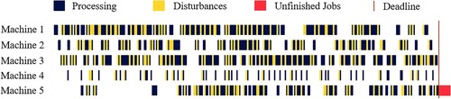
Figure 6. PV generation disturbance.

Graph comparing predicted and observed PV generation over time.

For $i=1,\dots ,288-k$. (11) $\{\begin{array}{l}{\hat{\mathbf{x}}}_6\left[k|k\right]\le {\theta }_9\\ {\hat{\mathbf{x}}}_7\left[k|k\right]\le {\theta }_9\\ {\hat{\mathbf{x}}}_8\left[k|k\right]\ge {\theta }_7\cdot (1-{\theta }_8)/2\\ {\hat{\mathbf{x}}}_8\left[k|k\right]\le {\theta }_7\cdot (1+{\theta }_8)/2\\ {\hat{\mathbf{x}}}_8\left[k|k\right]={\hat{\mathbf{x}}}_8\left[k|k\right]+{\theta }_4\cdot {\hat{\mathbf{x}}}_6\left[k|k\right]\\ -1/{\theta }_4\cdot {\hat{\mathbf{x}}}_7\left[k|k\right]\\ {\hat{\mathbf{x}}}_1\left[k\right]+{\hat{\mathbf{x}}}_9\left[k|k\right]+{\hat{\mathbf{x}}}_7\left[k|k\right]+{\hat{\mathbf{x}}}_5\left[k\right]\\ ={\displaystyle \sum _{m=1}^5{\hat{\mathbf{x}}}_{2,m}\left[k\right]\cdot {\mathit{\theta }}_{1,m}+{\hat{\mathbf{x}}}_5\left[k\right]+{\hat{\mathbf{x}}}_7\left[k|k\right]}\end{array}$(11)

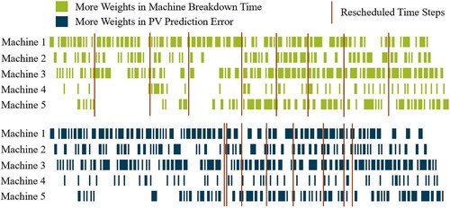
Thirdly, in S3, We design the performance evaluation function according to the sum of PV prediction error for the remainder of the day and accumulated production disturbance time. According to the result, the rescheduling instants are at 32nd, 72nd, 100th, 138th, 163rd, 186th, 211st and 242nd time steps.

Fourthly, S4 is conducted at the 5 time steps above. The objective function and constraints are shown below from (12(12) $\begin{array}{rl}{\mathbf{l}}_{4,k}& ={\hat{\mathbf{x}}}_9[k+i|k]\cdot {\mathit{\theta }}_{10,k}-{\hat{\mathbf{x}}}_{10}[k+i|k]\cdot {\theta }_{11}+{\theta }_5\\ & +\left({\hat{\mathbf{x}}}_6\right[k+i|k]+{\hat{\mathbf{x}}}_7[k+i|k\left]\right)\cdot {\theta }_4\\ & +{\hat{\mathbf{x}}}_5[k+i|k]\cdot {\theta }_3\end{array}$(12) )–(16(16) $\begin{array}{rl}& {\hat{\mathbf{x}}}_{4,m}[k+i|k]\\ & \ge {\hat{\mathbf{x}}}_{4,m+1}[k+i|k]+{\hat{\mathbf{x}}}_{2,m+1}[k+i|k],\\ & i=1,2,\dots ,288.\end{array}$(16) ).

Objective (12(12) $\begin{array}{rl}{\mathbf{l}}_{4,k}& ={\hat{\mathbf{x}}}_9[k+i|k]\cdot {\mathit{\theta }}_{10,k}-{\hat{\mathbf{x}}}_{10}[k+i|k]\cdot {\theta }_{11}+{\theta }_5\\ & +\left({\hat{\mathbf{x}}}_6\right[k+i|k]+{\hat{\mathbf{x}}}_7[k+i|k\left]\right)\cdot {\theta }_4\\ & +{\hat{\mathbf{x}}}_5[k+i|k]\cdot {\theta }_3\end{array}$(12) ) is the overall energy cost, including grid purchase cost, grid feed-in tariff, ESS usage cost and GaT generation cost. (12) $\begin{array}{rl}{\mathbf{l}}_{4,k}& ={\hat{\mathbf{x}}}_9[k+i|k]\cdot {\mathit{\theta }}_{10,k}-{\hat{\mathbf{x}}}_{10}[k+i|k]\cdot {\theta }_{11}+{\theta }_5\\ & +\left({\hat{\mathbf{x}}}_6\right[k+i|k]+{\hat{\mathbf{x}}}_7[k+i|k\left]\right)\cdot {\theta }_4\\ & +{\hat{\mathbf{x}}}_5[k+i|k]\cdot {\theta }_3\end{array}$(12) Constraints (13(13) $\begin{array}{rl}& \{\begin{array}{l}{\hat{\mathbf{x}}}_6[k+i|k]\le {\theta }_9\\ {\hat{\mathbf{x}}}_7[k+i|k]\le {\theta }_9\\ {\hat{\mathbf{x}}}_8[k+i|k]\ge {\theta }_7\cdot (1-{\theta }_8)/2\\ {\hat{\mathbf{x}}}_8[k+i|k]\le {\theta }_7\cdot (1+{\theta }_8)/2\\ {\hat{\mathbf{x}}}_8[k+i+1|k]\\ ={\hat{\mathbf{x}}}_8[k+i|k]+{\theta }_4\cdot {\hat{\mathbf{x}}}_6[k+i|k]\\ -1/{\theta }_4\cdot {\hat{\mathbf{x}}}_7[k+i|k]\\ {\hat{\mathbf{x}}}_1[k+i|k]+{\hat{\mathbf{x}}}_9[k+i|k]\\ +{\hat{\mathbf{x}}}_7[k+i|k]+{\hat{\mathbf{x}}}_5[k+i|k]\\ ={\displaystyle \sum _{m=1}^5{\hat{\mathbf{x}}}_{2,m}[k+i|k]\cdot {\mathit{\theta }}_{1,m}+{\hat{\mathbf{x}}}_{10}[k+i|k]}\\ +{\hat{\mathbf{x}}}_7[k+i|k]\end{array}\end{array}$(13) )–(16(16) $\begin{array}{rl}& {\hat{\mathbf{x}}}_{4,m}[k+i|k]\\ & \ge {\hat{\mathbf{x}}}_{4,m+1}[k+i|k]+{\hat{\mathbf{x}}}_{2,m+1}[k+i|k],\\ & i=1,2,\dots ,288.\end{array}$(16) ) have the same explanation as (6(6) $\{\begin{array}{l}{\hat{\mathbf{x}}}_6\left[i|0\right]\le {\theta }_9\\ {\hat{\mathbf{x}}}_7\left[i|0\right]\le {\theta }_9\\ {\hat{\mathbf{x}}}_8\left[i|0\right]\ge {\theta }_7\cdot (1-{\theta }_8)/2\\ {\hat{\mathbf{x}}}_8\left[i|0\right]\le {\theta }_7\cdot (1+{\theta }_8)/2\\ {\hat{\mathbf{x}}}_8[i+1|0]\\ ={\hat{\mathbf{x}}}_8\left[i|0\right]+{\theta }_4\cdot {\hat{\mathbf{x}}}_6\left[i|0\right]-1/{\theta }_4\cdot {\hat{\mathbf{x}}}_7\left[i|0\right]\\ {\hat{\mathbf{x}}}_1\left[i|0\right]+{\hat{\mathbf{x}}}_9\left[i|0\right]+{\hat{\mathbf{x}}}_7\left[i|0\right]+{\hat{\mathbf{x}}}_5\left[i|0\right]\\ ={\displaystyle \sum _{m=1}^5{\hat{\mathbf{x}}}_{2,m}\left[i|0\right]\cdot {\mathit{\theta }}_{1,m}+{\hat{\mathbf{x}}}_5\left[i|0\right]+{\hat{\mathbf{x}}}_7\left[i|0\right]}\end{array}$(6) )–(9(9) $\begin{array}{rl}{\hat{\mathbf{x}}}_{4,m}\left[i|0\right]& \ge {\hat{\mathbf{x}}}_{4,m+1}\left[i|0\right]+{\hat{\mathbf{x}}}_{2,m+1}\left[i|0\right],\\ & i=1,2,\dots ,288.\end{array}$(9) ), while all the starting time becomes the current time step, and the scheduling horizon covers the remainder of the day. For any $i=1,\dots ,287-k$: (13) $\begin{array}{rl}& \{\begin{array}{l}{\hat{\mathbf{x}}}_6[k+i|k]\le {\theta }_9\\ {\hat{\mathbf{x}}}_7[k+i|k]\le {\theta }_9\\ {\hat{\mathbf{x}}}_8[k+i|k]\ge {\theta }_7\cdot (1-{\theta }_8)/2\\ {\hat{\mathbf{x}}}_8[k+i|k]\le {\theta }_7\cdot (1+{\theta }_8)/2\\ {\hat{\mathbf{x}}}_8[k+i+1|k]\\ ={\hat{\mathbf{x}}}_8[k+i|k]+{\theta }_4\cdot {\hat{\mathbf{x}}}_6[k+i|k]\\ -1/{\theta }_4\cdot {\hat{\mathbf{x}}}_7[k+i|k]\\ {\hat{\mathbf{x}}}_1[k+i|k]+{\hat{\mathbf{x}}}_9[k+i|k]\\ +{\hat{\mathbf{x}}}_7[k+i|k]+{\hat{\mathbf{x}}}_5[k+i|k]\\ ={\displaystyle \sum _{m=1}^5{\hat{\mathbf{x}}}_{2,m}[k+i|k]\cdot {\mathit{\theta }}_{1,m}+{\hat{\mathbf{x}}}_{10}[k+i|k]}\\ +{\hat{\mathbf{x}}}_7[k+i|k]\end{array}\end{array}$(13) (14) $\begin{array}{rl}& \{\begin{array}{l}{\hat{\mathbf{x}}}_8\left[288|k\right]={\theta }_7\cdot 0.5\\ {\hat{\mathbf{x}}}_{4,5}\left[288|k\right]\ge {\theta }_{14}.\end{array}\end{array}$(14) For $m=1,\dots ,5$. (15) $\{\begin{array}{ll}{\hat{\mathbf{x}}}_{4,m}[k+i|k]=0,& i=1,2,\dots ,{\mathit{\theta }}_{2,m}.\\ {\hat{\mathbf{x}}}_{4,m}[k+i|k]& \\ ={\displaystyle \sum _{j=0}^{k-{\theta }_{2,m}}{\hat{\mathbf{x}}}_{3,m}[k+j|k],}& i={\mathit{\theta }}_{2,m},\dots ,288-k\\ {\hat{\mathbf{x}}}_{2,m}[k+i|k]& \\ ={\displaystyle \sum _{j=0}^k{\hat{\mathbf{x}}}_{3,m}[k+j|k],}& i=1,2,\dots ,{\mathit{\theta }}_{2,m}\\ {\hat{\mathbf{x}}}_{2,m}[k+i-1|k]& \\ ={\displaystyle \sum _{j=i-{\theta }_{2,m}}^k{\hat{\mathbf{x}}}_{3,m}[k+j|k],}& i={\mathit{\theta }}_{2,m},\dots ,288-k\\ {\hat{\mathbf{x}}}_{3,m}[k+i|k]\cdot {\mathit{\theta }}_{2,m}& \\ \le {\displaystyle \sum _{j=i}^{k+{\theta }_{2,m}}{\hat{\mathbf{x}}}_{2,m}[k+j|k],}& i=1,2,\dots ,288\\ & -k-{\mathit{\theta }}_{2,m}.\end{array}$(15) For $m=1,\dots ,5$ (16) $\begin{array}{rl}& {\hat{\mathbf{x}}}_{4,m}[k+i|k]\\ & \ge {\hat{\mathbf{x}}}_{4,m+1}[k+i|k]+{\hat{\mathbf{x}}}_{2,m+1}[k+i|k],\\ & i=1,2,\dots ,288.\end{array}$(16) Finally, after all of 4 steps, we can achieve the performance shown in Table 3. In the following scenarios, standard ETHS will be compared with other results.

Table 3. Result of standard ETHS.

Energy cost per product ($)	Finished products	Computational time (s)	Rescheduling frequency
1.77	50	117	8

4.3. Scenario 1: comparison with traditional methods

In this scenario, we compare ETHS with the traditional methods mentioned in Figure 2. The selected traditional methods include off-line scheduling (T1), hybrid scheduling with on-line optimisation model (T4) and hybrid scheduling with on-line heuristic model (T5). On-line methods are not compared because the on-line methods are included in hybrid methods. In T1, off-line schedules will be exactly followed, if the production is disturbed, the job will be postponed. In T4, the heuristic logistic is that all the change in supply and demand energy will be absorbed by ESS, if it exceeds the ESS power limit, the grid will compensate for the change. In T5, we execute off-line scheduling and reschedule it in real-time every hour. Results are shown in Table 4 and Figure 7.

Figure 7. Schedule comparison with traditional methods.

Four production schedules showing that ETHS and T4 are able to complete the production task while T1 and T5 can't.

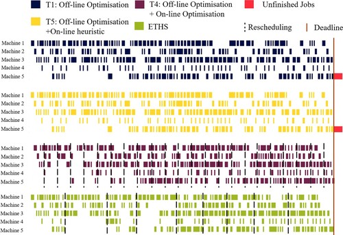
Table 4. Performance comparison with traditional methods.

Scenario	Energy cost per product ($)	Finished products	Computational time (s)
Standard ETHS	1.77	50	117
T1	2.49	48.3	3
T4	2.16	50	330
T5	1.83	48.3	8

According to the comparison results, T1 cannot finish the task on time, T4 can finish the task on time but the energy cost and computational time are higher because the highly flexible components are not utilised separately and the rescheduling frequency is fixed as once per hour. T5 reduces energy costs but cannot finish the task on time because the production schedule is not updated. Compared to the 3 methods above, ETHS achieves a balance between performance, robustness and computational cost. The reason for the outstanding results of ETHS will be analysed in scenario 2.

4.4. Scenario 2: sensitivity of each step in ETHS

In this scenario, we identify the essential function of S2, S3 and S4 via conducting a sensitivity analysis, where we remove each step and compare the results with standard ETHS. The comparison can be found in Table 5.

Table 5. Sensitivity Analysis of S2, S3 and S4.

Scenario	Energy cost per product ($)	Finished products	Computational time (s)
Standard ETHS	1.77	50	117
Remove S2	2.22	50	112
Remove S3	1.69	50	4152
Remove S4	1.83	48.3	8

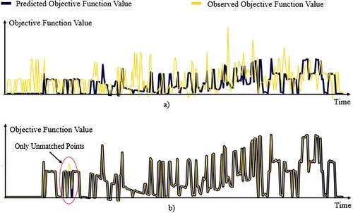
In the implemented ETHS, S2 is eliminated by utilising the ESS schedule generated by S1 and S4. The result shows that energy cost increases by $25.4\mathrm{\%}$, while the computational time and finished products are not influenced significantly. Meanwhile, S2 is utilising the highly flexible components to approach the optimised schedules calculated in S1 and S4 under disturbances, which is the reason that S2 can help achieve better performance. We compare the predicted and observed objective function values with S2 and without S2 in Figure 8, showing that S2 can significantly contribute to approaching the optimised schedules. In this case, the reason for unmatched points is that 5 machines are disturbed simultaneously, which results in a consumption power decrease, therefore the BESS achieves its power limit in discharging. The capacity of fully-dispatchable components determines how much S2 can contribute to approaching the predicted objective function value, which will be discussed in Section 4.5.

Figure 8. Gap between predicted and observed objective function value.

Graphs showing that with S2 the gap between observed and predicted objective function value can be reduced significantly.

Next, S3 is removed by using S4 at each time step without the event-trigger mechanism. The result shows that computational time increases by $3449\mathrm{\%}$, while the energy cost and finished products are not influenced significantly.

Finally, we remove S4 by following the off-line schedule for production and GaT and controlling ESS to minimise the objective function value gap. The result shows that the production task cannot be finished on time.

In conclusion, the ETHS framework plays a crucial role in balancing energy cost, production task completion, and computing time. It achieves this by integrating four steps, each contributing to the overall effectiveness of the approach. By leveraging the advantages of the three scheduling problems, ETHS yields satisfactory results in terms of system performance and optimisation.

4.5. Scenario 3: the role of component categorisation

In this scenario, we study the effect of selecting different partially-dispatchable components and fully-dispatchable components. Non-dispatchable components are fixed, including PV and grid. We compare the results with an increased number of fully-dispatchable components, from ESS only, to ESS and GaT, to ESS, GaT and the powder coating machine, the results are summarised in Table 6.

Table 6. Selection of different component categories.

Fully-dispatchable Components	Energy cost/ product	Finished products	Number of matching objective reference
Grid, ESS	1.77	50	284/288
Grid, ESS, GaT	1.75	50	288/288
Grid, ESS, GaT and powder coating machine	1.75	50	288/288

Since the function of fully-dispatchable components is handling disturbances when rescheduling is not needed, the more fully-dispatchable components have more capacity to handle the disturbance, which is reflected in Table 6. More objective function values can be controlled exactly the same as the predicted values with more fully-dispatchable components, and when all the predicted values can be approached, more fully-dispatchable components will not influence the performance.

4.6. Scenario 4: event-trigger mechanism

In this scenario, we investigate how to choose the event-trigger mechanism to determine when the rescheduling is needed and how many reschedules are suitable. In particular, we provide two methods to control the rescheduling instants and rescheduling frequency.

The first method is changing the parameters in the performance evaluation function, which means the weights for each rescheduling factor can be changed. Here if we focus more on the PV prediction error, the rescheduling instants are more likely to fall in the instants with high PV prediction error; if we focus more on the production disturbance time, the rescheduling instants are more likely to fall in the instants with accumulated longer production disturbance time, the comparison between two schedules is shown in Figure 9.

Figure 9. Reschedule time steps comparison between two performance evaluation functions.

Graphs showing that different weights in S3 can result in different rescheduling time steps.

The second method is changing the threshold in S3, a higher threshold means more frequent rescheduling, The comparison between three different threshold settings is shown in Table 7. With the increasing of threshold, the energy cost increases but the rescheduling frequency and computational time decreases.

Table 7. Threshold comparison.

Threhold	Finished products	Energy cost per product ($)	Computing time ($)	Reschedule frequency
$ϵ=25$	50	1.73	213	16
$ϵ=45$	50	1.77	117	8
$ϵ=65$	50	1.80	86	6

With the combination of two methods, the user of ETHS can adjust the rescheduling instants and frequency according to their requirements and the performance of the system.

In summary, the case study presented in this paper provides a clear demonstration of how to implement the proposed ETHS framework in a factory setting. The scenarios presented validate the functionality of each step in ETHS and highlight its ability to achieve a balance between system performance, production efficiency, and computational cost.

Scenario 0 serves as a practical example of implementing ETHS in a factory, showcasing its effectiveness in managing the scheduling of various components.

Scenario 1 demonstrates the importance of each step. Scenario 2 emphasises the importance of accurately categorising components based on their physical properties and system requirements. Scenario 3 introduces methods for controlling the timing and frequency of rescheduling, offering insights into strategies for managing the dynamic nature of the integrated system.

The case study as a whole provides valuable insights into the implementation of ETHS, including the design of variables and parameters within the system. The findings have the potential to be applied in a wide range of factories, demonstrating the practical applicability and flexibility of ETHS in real-world settings.

The ETHS case study reveals three key managerial advantages:

Optimised Energy Efficiency:

ETHS strategically deploys fully-dispatchable components, particularly within Renewable Energy Sources (RESs), enhancing energy efficiency for cost-effective and sustainable manufacturing.

Operational Stability:

ETHS integrates real-time disturbance handling and dynamic performance evaluation, minimising production interruptions and ensuring stable operations.

Adaptability and Flexibility:

With design freedoms, ETHS offers adaptability across manufacturing environments, empowering managers to implement a scalable solution tailored to specific needs.

5. Conclusion

This paper proposes a systematic design framework of Event-triggered Hybrid Scheduling (ETHS) to address the balance between robustness and computational cost of energy-aware scheduling for manufacturing factories integrated with renewables. It is a four-step procedure that includes off-line scheduling, on-line adjustment, performance evaluation, and on-line rescheduling by carefully exploring the flexibility of the integrated system.

A case study from the real manufacturing industry is presented to validate ETHS in a real production environment, demonstrating its effectiveness, the importance of each step, and the design freedom in this framework including component categorisation, rescheduling instants and frequency.

For future investigation, it is advisable to explore a more intricate production environment to showcase the practicality of ETHS. Additionally, there should be a deliberate exploration into utilising models of varying complexity within this framework.

Disclosure statement

No potential conflict of interest was reported by the author(s).

Data availability statement

The data that support the findings of this study are available from the corresponding author, [Li], upon reasonable requests.

Additional information

Notes on contributors

Zhean Shao

Zhean Shao is a PhD candidate in the Department of Mechanical Engineering at the University of Melbourne. He earned his Bachelor's degree from Xi'an Jiao Tong University, China in 2020 and joined the Manufacturing and Industrial Engineering Group at the University of Melbourne in 2021. His research focuses on industrial digital twins for enabling energy-efficient manufacturing systems with energy-aware scheduling and renewable energy management. His research critically addresses the uncertainties inherent in manufacturing environments, devising solutions to mitigate their impact and enhance system resilience.

Wen Li

Wen Li Dr. is an associate professor in the Department of Mechanical Engineering at the University of Melbourne. He earned his PhD from the University of New South Wales in 2012. He is the funding academic of the Manufacturing and Industrial Systems Engineering group at the University of Melbourne. His research interests include energy and eco-efficiency in manufacturing, life cycle analysis, industrial IoT for cleaner production, supply chain traceability, as well as material criticality. Dr Li has extensive experience in working with diverse industries, including automotive, mining and processing, transportation, pharmaceuticals, construction, and food and beverage.

Ying Tan

Ying Tan Dr. is a Professor in the Department of Mechanical Engineering at The University of Melbourne, Australia. She received her Bachelor's degree from Tianjin University, China, in 1995, and her PhD from the National University of Singapore in 2002. She joined McMaster University in 2002 as a postdoctoral fellow in the Department of Chemical Engineering. Since 2004, she has been with the University of Melbourne. She was awarded an Australian Postdoctoral Fellow (2006–2008) and a Future Fellow (2009–2013) by the Australian Research Council. She is Fellow of the Institute of Electrical and Electronic Engineers (FIEEE), Fellow of the Institution of Engineers of Australia (FIEAUST), and Fellow of Asia-Pacific Artificial Intelligence Association. Her research interests are in intelligent systems, nonlinear systems, real-time optimisation, sampled-data systems, rehabilitation robotic systems, human motor learning, wearable sensors, and model-guided machine learning.

Kevin Otto

Kevin Otto Dr. is a Professor in the Manufacturing and Industrial Engineering Group in the Department of Mechanical Engineering at the University of Melbourne. Professor Otto is an expert in design and manufacturing quality improvement and flexible modular design. His research expertise has been in uncertainty quantification and optimisation to reduce production variability using both on-line and off-line modelling and experimentation. This includes robust design optimisation to ensure confidence levels against probabilistic risk of performance compliance. He has particular interest in model calibration, uncertainty quantification from multiple sources including test and fabrication, and the study of variability reduction across modular product families.

References

- Abikarram, Jose Batista, and Katie McConky. 2017. “Real Time Machine Coordination for Instantaneous Load Smoothing and Photovoltaic Intermittency Mitigation.” Journal of Cleaner Production 142: 1406–1416. https://doi.org/10.1016/j.jclepro.2016.11.166.
- Akbar, Muhammad, and Takashi Irohara. 2018. “Scheduling for Sustainable Manufacturing: A Review.” Journal of Cleaner Production 205: 866–883. https://doi.org/10.1016/j.jclepro.2018.09.100.
- Alfieri, A. 2007. “Due Date Quoting and Scheduling Interaction in Production Lines.” International Journal of Computer Integrated Manufacturing 20 (6): 579–587. https://doi.org/10.1080/09511920601079363.
- Allahverdi, Ali, and Harun Aydilek. 2010. “Heuristics for the Two-Machine Flowshop Scheduling Problem to Minimize Maximum Lateness With Bounded Processing Times.” Computers and Mathematics with Applications 60 (5): 1374–1384. https://doi.org/10.1016/j.camwa.2010.06.019.
- Alturki, Fahd A., and Emad Mahrous Awwad. 2021. “Sizing and Cost Minimization of Standalone Hybrid WT/PV/Biomass/Pump-Hydro Storage-Based Energy Systems.” Energies 14 (2): 489. https://doi.org/10.3390/en14020489.
- Bänsch, Kristian, Jan Busse, Frank Meisel, Julia Rieck, Sebastian Scholz, Thomas Volling, and Matthias G. Wichmann. 2021. “Energy-Aware Decision Support Models in Production Environments: A Systematic Literature Review.” Computers and Industrial Engineering 159: 107456. https://doi.org/10.1016/j.cie.2021.107456.
- Beier, Jan. 2017. Simulation Approach Towards Energy Flexible Manufacturing Systems. Sustainable Production, Life Cycle Engineering and Management. Cham: Springer International Publishing. https://doi.org/10.1007/978-3-319-46639-2.
- Biel, Konstantin, Fu Zhao, John W. Sutherland, and Christoph H. Glock. 2018. “Flow Shop Scheduling With Grid-Integrated Onsite Wind Power Using Stochastic MILP.” International Journal of Production Research 56 (5): 2076–2098. https://doi.org/10.1080/00207543.2017.1351638.
- Bruzzone, A. A. G., D. Anghinolfi, M. Paolucci, and F. Tonelli. 2012. “Energy-Aware Scheduling for Improving Manufacturing Process Sustainability: A Mathematical Model for Flexible Flow Shops.” CIRP Annals 61 (1): 459–462. https://doi.org/10.1016/j.cirp.2012.03.084.
- Cai, Lei, Wenfeng Li, Yun Luo, and Lijun He. 2023. “Real-Time Scheduling Simulation Optimisation of Job Shop in A Production-Logistics Collaborative Environment.” International Journal of Production Research 61 (5): 1373–1393. https://doi.org/10.1080/00207543.2021.2023777.
- Caldeira, Rylan H., A. Gnanavelbabu, and T. Vaidyanathan. 2020. “An Effective Backtracking Search Algorithm for Multi-Objective Flexible Job Shop Scheduling Considering New Job Arrivals and Energy Consumption.” Computers and Industrial Engineering 149: 106863. https://doi.org/10.1016/j.cie.2020.106863.
- Carlucci, Daniela, Paolo Renna, and Sergio Materi. 2023. “A Job-Shop Scheduling Decision-Making Model for Sustainable Production Planning With Power Constraint.” IEEE Transactions on Engineering Management 70 (5): 1923–1932. https://doi.org/10.1109/TEM.2021.3103108.
- Chowdhury, S., G. A. Taylor, S. P. Chowdhury, A. K. Saha, and Y. H. Song. 2007. “Modelling, Simulation and Performance Analysis of a PV Array in An Embedded Environment.” In 2007 42nd International Universities Power Engineering Conference, 781–785. IEEE.
- Dong, Jun, and Chunming Ye. 2022. “Green Scheduling of Distributed Two-Stage Reentrant Hybrid Flow Shop Considering Distributed Energy Resources And Energy Storage System.” Computers and Industrial Engineering 169: 108146. https://doi.org/10.1016/j.cie.2022.108146.
- Eunike, Agustina, Kung-Jeng Wang, Jingming Chiu, and Yuling Hsu. 2022. “Real-Time Resilient Scheduling by Digital Twin Technology in a Flow-Shop Manufacturing System.” Procedia CIRP 107: 668–674. https://doi.org/10.1016/j.procir.2022.05.043.
- Fang, Kuei-Tang, and Bertrand M. T. Lin. 2013. “Parallel-Machine Scheduling to Minimize Tardiness Penalty and Power Cost.” Computers & Industrial Engineering 64 (1): 224–234. https://doi.org/10.1016/j.cie.2012.10.002.
- Hasan, S. M. Kamrul, Ruhul Sarker, and Daryl Essam. 2011. “Genetic Algorithm for Job-Shop Scheduling With Machine Unavailability and Breakdowns.” International Journal of Production Research 49 (16): 4999–5015. https://doi.org/10.1080/00207543.2010.495088.
- Karimi, Sajad, and Soongeol Kwon. 2021. “Comparative Analysis of the Impact of Energy-Aware Scheduling, Renewable Energy Generation, and Battery Energy Storage on Production Scheduling.” International Journal of Energy Research 45 (13): 18981–18998. https://doi.org/10.1002/er.6999.
- Katragjini, Ketrina, Eva Vallada, and Rubén Ruiz. 2013. “Flow Shop Rescheduling Under Different Types of Disruption.” International Journal of Production Research 51 (3): 780–797. https://doi.org/10.1080/00207543.2012.666856.
- Kemmoe, Sylverin, Damien Lamy, and Nikolay Tchernev. 2017. “Job-Shop Like Manufacturing System With Variable Power Threshold and Operations With Power Requirements.” International Journal of Production Research 55 (20): 6011–6032. https://doi.org/10.1080/00207543.2017.1321801.
- Khalaf, Alireza Fazli, and Yong Wang. 2018. “Energy-Cost-Aware Flow Shop Scheduling Considering Intermittent Renewables, Energy Storage, And Real-Time Electricity Pricing.” International Journal of Energy Research 42 (12): 3928–3942. https://doi.org/10.1002/er.4130.
- Khaled, Mohamed Saeed, Ibrahim Abdelfadeel Shaban, Ahmed Karam, Mohamed Hussain, Ismail Zahran, and Mohamed Hussein. 2022. “An Analysis of Research Trends in the Sustainability of Production Planning.” Energies 15 (2): 483. https://doi.org/10.3390/en15020483.
- Kim, Hyun-Jung, Eun-Seok Kim, Jun-Ho Lee, Lixin Tang, and Yang Yang. 2022. “Single-Machine Scheduling With Energy Generation and Storage Systems.” International Journal of Production Research 60 (23): 7033–7052. https://doi.org/10.1080/00207543.2021.2000655.
- Kumar, K. Prakash, and B. Saravanan. 2017. “Recent Techniques to Model Uncertainties in Power Generation From Renewable Energy Sources and Loads in Microgrids – A Review.” Renewable and Sustainable Energy Reviews 71: 348–358. https://doi.org/10.1016/j.rser.2016.12.063.
- Lee, Seokgi, and Vittaldas V. Prabhu. 2015. “Energy-Aware Feedback Control for Production Scheduling and Capacity Control.” International Journal of Production Research 53 (23): 7158–7170. https://doi.org/10.1080/00207543.2015.1082666.
- Li, Wen. 2015. Efficiency of Manufacturing Processes: Energy and Ecological Perspectives. Sustainable Production, Life Cycle Engineering and Management. Cham: Springer International Publishing. https://doi.org/10.1007/978-3-319-17365-8.
- Liu, Cheng-Hsiang. 2016. “Mathematical Programming Formulations for Single-Machine Scheduling Problems While Considering Renewable Energy Uncertainty.” International Journal of Production Research 54 (4): 1122–1133. https://doi.org/10.1080/00207543.2015.1048380.
- Liu, Guo-Sheng, Hai-Dong Yang, and Ming-Bao Cheng. 2017. “A Three-Stage Decomposition Approach for Energy-Aware Scheduling With Processing-Time-Dependent Product Quality.” International Journal of Production Research 55 (11): 3073–3091. https://doi.org/10.1080/00207543.2016.1241446.
- Mikhaylidi, Yevgenia, Hussein Naseraldin, and Liron Yedidsion. 2015. “Operations Scheduling Under Electricity Time-Varying Prices.” International Journal of Production Research 53 (23): 7136–7157. https://doi.org/10.1080/00207543.2015.1058981.
- Moon, Joon-Yung, and Jinwoo Park. 2014. “Smart Production Scheduling With Time-Dependent and Machine-Dependent Electricity Cost by Considering Distributed Energy Resources and Energy Storage.” International Journal of Production Research 52 (13): 3922–3939. https://doi.org/10.1080/00207543.2013.860251.
- Mouzon, Gilles, Mehmet B. Yildirim, and Janet Twomey. 2007. “Operational Methods for Minimization of Energy Consumption of Manufacturing Equipment.” International Journal of Production Research 45 (18–19): 4247–4271. https://doi.org/10.1080/00207540701450013.
- Nayak, Ashutosh, Seokcheon Lee, and John W. Sutherland. 2019. “Dynamic Load Scheduling for Energy Efficiency in a Job Shop With On-Site Wind Mill for Energy Generation.” Procedia CIRP 80: 197–202. https://doi.org/10.1016/j.procir.2018.12.003.
- Nouiri, M., A. Bekrar, and D. Trentesaux. 2018. “Towards Energy Efficient Scheduling and Rescheduling for Dynamic Flexible Job Shop Problem.” IFAC-PapersOnLine 51 (11): 1275–1280. https://doi.org/10.1016/j.ifacol.2018.08.357.
- Pei, Zhi, Peiqi Yang, Yujuan Wang, and Chao-Bo Yan. 2023. “Energy Consumption Control in the Two-machine Bernoulli Serial Production Line With Setup and Idleness.” International Journal of Production Research 61 (9): 2917–2936. https://doi.org/10.1080/00207543.2022.2073287.
- Ren, Jianfeng, Chunming Ye, and Feng Yang. 2021. “Solving Flow-shop Scheduling Problem With a Reinforcement Learning Algorithm That Generalizes the Value Function With Neural Network.” Alexandria Engineering Journal 60 (3): 2787–2800. https://doi.org/10.1016/j.aej.2021.01.030.
- Salido, Miguel A., Joan Escamilla, Federico Barber, and Adriana Giret. 2017. “Rescheduling in Job-shop Problems for Sustainable Manufacturing Systems.” Journal of Cleaner Production 162: S121–S132. https://doi.org/10.1016/j.jclepro.2016.11.002.
- Sang, Yanwei, Jianping Tan, and Wen Liu. 2021. “A New Many-objective Green Dynamic Scheduling Disruption Management Approach for Machining Workshop Based on Green Manufacturing.” Journal of Cleaner Production 297: 126489. https://doi.org/10.1016/j.jclepro.2021.126489.
- Shi, Jiaqi, Liya Ma, Chenchen Li, Nian Liu, and Jianhua Zhang. 2022. “A Comprehensive Review of Standards for Distributed Energy Resource Grid-integration and Microgrid.” Renewable and Sustainable Energy Reviews 170: 112957. https://doi.org/10.1016/j.rser.2022.112957.
- Thornton, Ashley, Cedric Schultz, Sami Kara, and Gunther Reinhart. December 2017. “Concurrent scheduling of a job shop and microgrid to minimize energy costs under due date constraints.” In 2017 IEEE International Conference on Industrial Engineering and Engineering Management (IEEM), 1326–1330. Singapore: IEEE. http://ieeexplore.ieee.org/document/8290108/.
- Wang, Kai, Yun Huang, and Hu Qin. 2016. “A Fuzzy Logic-based Hybrid Estimation of Distribution Algorithm for Distributed Permutation Flowshop Scheduling Problems Under Machine Breakdown.” Journal of the Operational Research Society 67 (1): 68–82. https://doi.org/10.1057/jors.2015.50.
- Wang, Jin, Yang Liu, Shan Ren, Chuang Wang, and Wenbo Wang. 2021. “Evolutionary Game Based Real-time Scheduling for Energy-efficient Distributed and Flexible Job Shop.” Journal of Cleaner Production 293: 126093. https://doi.org/10.1016/j.jclepro.2021.126093.
- Xiong, Jian, Li-ning Xing, and Ying-wu Chen. 2013. “Robust Scheduling for Multi-objective Flexible Job-shop Problems With Random Machine Breakdowns.” International Journal of Production Economics 141 (1): 112–126. https://doi.org/10.1016/j.ijpe.2012.04.015.
- Yan, Qi, Hongfeng Wang, and Fang Wu. 2022. “Digital Twin-enabled Dynamic Scheduling With Preventive Maintenance Using a Double-layer Q-learning Algorithm.” Computers and Operations Research 144: 105823. https://doi.org/10.1016/j.cor.2022.105823.
- Zhai, Yuxin, Konstantin Biel, Fu Zhao, and John W. Sutherland. 2017. “Dynamic Scheduling of a Flow Shop With On-Site Wind Generation for Energy Cost Reduction Under Real Time Electricity Pricing.” CIRP Annals 66 (1): 41–44. https://doi.org/10.1016/j.cirp.2017.04.099.