Optimisation of recovery policies in the era of supply chain disruptions: a system dynamics and reinforcement learning approach

Abstract

Incidents like the COVID-19 pandemic or military conflicts disrupted global supply chains, causing long-lasting shortages in multiple sectors. This so-called ripple effect denotes the propagation of disruptions to further elements of the supply chain. Due to the severity of the impact that the ripple effect has on revenues, service levels, and reputation among supply chain entities, it is essential to understand the related implications. Given the unpredictable nature of disrupting events, this study emphasises the value of a reactive development of effective recovery policies on an operational level. In this article, a system dynamics model for a supply chain is used as framework to investigate the ripple effect. Based on this model, recovery policies are generated using reinforcement learning (RL), which represents a novel approach in this context. As main findings, the experimental results demonstrate the applicability of the proposed approach in mitigating the ripple effect based on secondary data from a major aerospace and defence supply chain and furthermore, the results indicate a broad applicability of the approach without the need for complete information about the disruption characteristics and supply chain entities. With further refinement and real-world implementation, the presented approach provides the potential to enhance supply chain resilience in practice.

Keywords:

• Supply chain disruption
• ripple effect
• system dynamics
• reinforcement learning
• simulation optimisation

Sustainable Development Goals:

• SDG 12: Responsible consumption and production

1. Introduction

A disruption can be defined as an unplanned event, that has a significant impact on companies' operations in a negative way (Sinha, Bagodi, and Dey 2020), and arises in the upstream supply chain, in inbound logistics, or in the sourcing environment (Golan, Jernegan, and Linkov 2020). More than half of the companies worldwide face a supply chain disruption every year (Katsaliaki, Galetsi, and Kumar 2022), occurring as point load (e.g. a natural disaster, Ukraine war) or as distributed load (e.g. COVID pandemic, economic recession) (Golan, Jernegan, and Linkov 2020). Current trends regarding lean inventories (Golan, Jernegan, and Linkov 2020; Sinha, Bagodi, and Dey 2020), globalisation, outsourcing, and specialisation increase the vulnerability of supply chains for shortages (Ivanov 2019) and are a potential lever for the so called ripple effect (Dolgui, Ivanov, and Sokolov 2018; Katsaliaki, Galetsi, and Kumar 2022). This effect denotes the situation when a disruption does not remain localised in one point, but also is propagated to other entities of the supply chain (Dolgui, Ivanov, and Sokolov 2018; Ivanov 2019). Due to the order of magnitude this effect has on revenues, service levels, market share, and reputation of members of the supply chain it is essential to understand the implications of the ripple effect (Dolgui, Ivanov, and Sokolov 2018). As most disruption-triggering events are unpredictable and located outside of the influence sphere of the respective supply chain members, it is suggested to focus on managing and understanding the effects instead of trying to identify and eliminate the root causes of disruptions (Dolgui, Ivanov, and Sokolov 2018; Katsaliaki, Galetsi, and Kumar 2022; Olivares-Aguila and ElMaraghy 2021). Apart from structural interventions with the aim of increasing organisational resilience against disruptions, mitigation can be achieved by speeding up recovery on operational levels (Jaenichen et al. 2021). Since inventory is a major cost driver in supply chains (Timme and Williams-Timme 2003), an important approach for operational recovery are adaptive order policies that support a quick normalisation of service and inventory levels (Schmitt et al. 2017). To investigate the effects of disruptions and order policies in the supply chain, simulation, and in particular system dynamics, have shown to be an efficient tool for decision making and risk evaluation (Gu and Gao 2017; Mortazavi, Khamseh, and Azimi 2015; Olivares-Aguila and ElMaraghy 2021). Suitable recovery policies are derived from the simulation usually with the help of different ”what-if” scenarios (Dolgui, Ivanov, and Sokolov 2018). To avoid this time-consuming scenario building, the combination of simulation models with optimisation algorithms has gained attention, which is expected to have a significant impact on supply chain management (SCM) in the future (Ivanov et al. 2019; Tordecilla et al. 2021). However, due to the stochastic and dynamic properties of supply chains, many optimisation techniques are not applicable for generating order policies (Ivanov et al. 2016; Mortazavi, Khamseh, and Azimi 2015) and additional research is needed (Schmitt et al. 2017). A frequently applied optimisation approach for simulations are metaheuristics (Tordecilla et al. 2021), but the quality of obtained solutions often is not sufficient in the SCM context (Schmitt et al. 2017). Reinforcement learning (RL) is one of the most efficient techniques to solve dynamic optimisation problems and was successfully applied for learning order policies (Rolf et al. 2023; Yan et al. 2022). Thus, system dynamics and RL are promising approaches for ripple effect mitigation through order policies, but research on the integration of both is limited to a proof-of-concept solution proposed by Rahmandad and Fallah-Fini (2008). In general, there is a research gap regarding digital twin-based supply chain simulation and optimisation for disruption mitigation through recovery policies (Katsaliaki, Galetsi, and Kumar 2022), which motivates the integration of system dynamics and RL in a joint framework for this purpose. Both techniques have shown promising performance, and their integration provides the potential to learn robust order policies without the need for historical data, which is difficult to obtain for supply chain disruptions. With the proposed integration, order policies can be generated without information on time, duration, and location of the disruption and tedious scenario building can be avoided. The general capabilities of RL in high-dimensional action spaces (Kurian et al. 2022) make the approach also scalable to large supply chain models, the only requirement for applicability in practice is an accurate system dynamics model of the studied supply chain in the sense of a digital twin.

Motivated by the high probability of future supply chain disruptions, e.g. through ongoing climate change (Golan, Jernegan, and Linkov 2020), the integrated use of system dynamics and RL is proposed as a novel simulation-optimisation approach for disruption mitigation. For this, the main contributions of this paper are: (i) to build a system dynamics simulation model to analyse the behaviour of a supply chain under disruptions with regard to inventory levels and orders from existing approaches; (ii) to integrate an RL optimisation into the simulation model and to mitigate the ripple effect by robust recovery policies with a focus on intelligent ordering mechanisms; and (iii) to evaluate the utility of the proposed approach in different scenarios.

Section 2 outlines the state of the art of research regarding supply chain disruptions and recovery policies, their quantitative modelling, and optimisation possibilities. Based on the reviewed literature, in Section 3, a problem description is presented, which is followed in Section 4 by a delineation of the used system dynamics model to simulate the supply chain behaviour under disruptions. The optimisation approach using RL is introduced in Section 5, followed by an experimental application and evaluation of the proposed algorithmic framework in Section 6. The results are discussed in Section 7, in Section 8 managerial insights and theoretical implications are presented, and in Section 9 a summary is given and further research directions are outlined.

2. Literature review

To give an overview on the current state of the art of ripple effect mitigation, first, in Section 2.1, general characteristics of supply chain resilience and recovery are outlined. In Section 2.2, system dynamics models and RL approaches for the optimisation of supply chains under disruptions are reviewed.

2.1. Supply chain disruptions and recovery policies

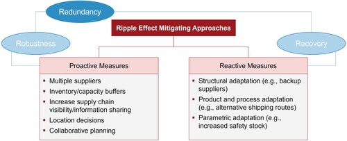
Driven by disrupting events like the COVID pandemic, the Ukraine war, or ongoing climate change, the objective of SCM shifted from pure efficiency towards an additional consideration of resilience against disruptions (Jaenichen et al. 2021). Although efficiency remains important for a supply chain's success (Golan, Jernegan, and Linkov 2020), enabling resilience will be a critical success factor for the future as competition among companies has been replaced by competition among supply chains (Jafarnejad et al. 2019). Resilience can be defined as the ability to prepare for, recover from, and adapt to adverse disruptions (Golan, Jernegan, and Linkov 2020). Measures to improve resilience and thus to handle disruptions can be classified into proactive and reactive approaches (Ivanov 2019; Olivares-Aguila and ElMaraghy 2021) (see Figure 1), which are related to supply chain robustness and recovery. Robustness describes the supply chain's ability to reduce the impact of disruptions whereas recovery describes the ability to recover fast from disruptions (Dolgui, Ivanov, and Sokolov 2018). To ensure robustness, possible example measures are multiple suppliers (Llaguno, Mula, and Campuzano-Bolarin 2022; Olivares-Aguila and ElMaraghy 2021), inventory buffers (Olivares-Aguila and ElMaraghy 2021), increasing supply chain visibility (Li and Zobel 2020), information sharing (Golan, Jernegan, and Linkov 2020), location decisions in consideration of resilience criteria (Olivares-Aguila and ElMaraghy 2021), and collaborative planning (Dolgui, Ivanov, and Sokolov 2018). Due to the unpredictability of disruptions, an operational and reactive management of their effects required in practice (Katsaliaki, Galetsi, and Kumar 2022). Reactive measures can be categorised in structural adaptation (e.g. the use of backup suppliers Ivanov et al. 2017; Llaguno, Mula, and Campuzano-Bolarin 2022), process adaptation (e.g. the use of alternative shipping routes (Dolgui, Ivanov, and Sokolov 2018)), as well as parametric adaptation (e.g. increased safety stock (Katsaliaki, Galetsi, and Kumar 2022)) (Dolgui, Ivanov, and Sokolov 2018; Ivanov et al. 2017). If several reactive and proactive measures are realised jointly, redundancy can be achieved, which enables a resilient supply chain capable to mitigate the ripple effect (Ivanov et al. 2017). In general, the concept of resilience is closely associated with flexibility of the supply chain, which can be seen as a driver enabling robust and rapidly recovering supply chains (Dolgui, Ivanov, and Sokolov 2018).

Figure 1. Ripple effect mitigating approaches (based on Dolgui, Ivanov, and Sokolov 2018).

A figure that lists exemplary proactive and reactive ripple effect mitigation approaches which should be applied simultaneously to achieve redundancy; proactive measures increase robustness while reactive measures improve recovery.

Since reactive measures are implemented after a disruption has occurred, they represent policies aimed at improving the recovery of the supply chain. These are often configured in form of contingency plans, which provide alternative suppliers or shipping routes, to be implemented quickly to avoid a long-term impact of the disruption (Ivanov et al. 2016). Parametric adaptation represents a simpler and more cost-effective approach where the recovery policy can be determined by adjusting critical parameters such as lead time, inventory control models (Ivanov et al. 2017), or adaptive and rush orders (Golan, Jernegan, and Linkov 2020; Ivanov et al. 2016). As a major aspect of supply chain dynamics, inventory levels and orders are influenced by disruptions and recovery policies. In turn, inventory levels and orders impact the supply chain behaviour and ripple effect severity. Therefore, a recovery policy in form of ordering model should be defined to manage a supply chain under disruptions (Ivanov 2017). Based on the expected duration and severity of a disruption, simulations of different recovery policies can be used to estimate their operational and financial impact, supporting managers to select the most appropriate one (Ivanov et al. 2017). Simulation thus enables a deeper understanding of the dynamic behaviour of supply chains under disruption and allows to evaluate the trade-off between resilience improvement and costs for the respective recovery policy (Golan, Jernegan, and Linkov 2020).

2.2. System dynamics and RL for supply chain optimisation

Simulation models are designed to mimic the behaviour of a real system. To derive recommendations from the simulation model, a series of runs is required, usually in form of a sensitivity analysis (Aslam and Ng 2016; Campuzano and Mula 2011). Simulation can be advantageous in situations where the observed system is highly complex (Olivares-Aguila and ElMaraghy 2021) or to test planned systems or changes in advance without involvement of a real system (Campuzano and Mula 2011). A common approach for the simulation of supply chain disruptions is system dynamics. This methodology is based on equation-based modelling and allows for the incorporation of non-linearities and feedback loops (Campuzano and Mula 2011). Unlike other simulation approaches, system dynamics enables modelling of a system at a high abstraction level, making simulations less computationally expensive and less prone to errors (Jaenichen et al. 2021). Feedback loops emerging from flows of information or material can be incorporated inherently, making system dynamics a well-suited approach for simulating supply chains (Aslam and Ng 2016).

In recent years, several studies were conducted that use system dynamics modelling to investigate the effects of disruptions on supply chains. An overview about the existing approaches is provided in Table 1. Regarding their target industry, no significant clusters could be observed but most approaches focus on manufacturing in general. Mostly, a size of three or four entities is assumed for the simulated supply chains. In one approach, that considers the supply chain as closed loop, a supply chain consisting of seven elements (supplier, producer, manufacturer, wholesaler, retailer, collector, disassembly centre) is simulated (Gu and Gao 2017). In one case, resilience is modelled independent from a specific supply chain directly by related variables like a level of agility or information sharing (Jafarnejad et al. 2019). The used key performance indicators (KPIs) varied across the different approaches. In three models, monetary objective values are used (Gu and Gao 2017; Jafarnejad et al. 2019; Llaguno, Mula, and Campuzano-Bolarin 2022; Olivares-Aguila and ElMaraghy 2021) (sales, cash reserves, profit, and cost, respectively). The other frequent approach is the usage of supply chain performance metrics as objectives, this can be a vulnerability index (Ghadge et al. 2022), a measure for supply chain agility (Jafarnejad et al. 2019), the service level (Olivares-Aguila and ElMaraghy 2021), or the capacity utilisation (Zhu, Krikke, and Caniëls 2021). Disruptions in the models are induced on different points of the supply chain, this can be a cut in demand (Ghadge et al. 2022; Gu and Gao 2017; Zhu, Krikke, and Caniëls 2021), supply (Ghadge et al. 2022; Llaguno, Mula, and Campuzano-Bolarin 2022; Zhu, Krikke, and Caniëls 2021), transport (Ghadge et al. 2022; Zhu, Krikke, and Caniëls 2021), or production capacities (Olivares-Aguila and ElMaraghy 2021). Independent variables that are used to mitigate or model the effects of disruptions can be demand and supply (Ghadge et al. 2022; Llaguno, Mula, and Campuzano-Bolarin 2022), inventory cover times (Gu and Gao 2017), disruption duration (Llaguno, Mula, and Campuzano-Bolarin 2022; Olivares-Aguila and ElMaraghy 2021), or information delay (Zhu, Krikke, and Caniëls 2021). In the majority of considered articles, different scenarios are built and compared as optimisation methodology, which is a common approach for simulation models. In two papers, only the effects of disruptions are quantified and visualised using the simulation models (Ghadge et al. 2022; Llaguno, Mula, and Campuzano-Bolarin 2022).

Table 1. Summary of recent approaches tackling supply chain disruptions with system dynamics.

	Model Characteristics
	Industry	SC Size	Objective/KPIs	Independent Variables	Disruption Characteristics	Optimisation Approach
Ghadge et al. (2022)	aerospace and defence	4 echelons (supplier, manufacturer, distributor, retailer)	vulnerability index	demand, supply (not sufficient material) and logistics risk (not sufficient transport capacities)	3 possibilities: disruption of demand, supply, or transport capacities	none, just quantifying disruption effects
Gu and Gao (2017)	manufacturing (closed-loop)	7 echelons(supplier, producer, manufacturer, wholesaler, retailer, collector, disassembly)	sales, sales ratio (sales 6 weeks after disruption/sales before disruption)	inventory cover time for manufacturer, wholesaler, and retailer	demand (given sequence by formula)	simulating scenarios
Jafarnejad et al. (2019)	medical equipment	modelling resilience without given supply chain	supply chain agility, level of risk management, cooperation level, cash reserves	creating different scenarios by deleting boundaries	none, modelling resilience directly	simulating scenarios
Llaguno, Mula, and Campuzano-Bolarin (2022)	manufacturing	3 echelons (manufacturer, wholesaler, retailer)	profit	disruption length, demand/supply between entities (SC and end customer)	disruption is a cut of supply for a defined time period	none, just quantifying disruption effects
Olivares-Aguila and ElMaraghy (2021)	manufacturing	4 echelons (tier-2 supplier, tier-1 supplier, plant, distributor)	service level, cost, (profit, inventory, backlog)	capacity decrease, disruption duration, expediting rate, expediting days	production capacity: partial and full disruption	simulating scenarios
Zhu, Krikke, and Caniëls (2021)	cheese industry	3 echelons (producer, logistics service provider, retailer)	capacity utilisation, retailer inventory, order backlog, shipment time, cumulative demand	information distortion, information delay	producer supply, transport, or demand interrupted	simulating scenarios

Instead of performing a tedious sensitivity analysis, recommendations can also be derived from a simulation model with the help of optimisation algorithms. This approach is referred to as simulation-optimisation (SimOpt) (Zhou and Zhou 2019). In the context of SCM, a frequently employed optimisation approach is RL. Applications of RL include several logistics problems, inventory replenishment, risk management, pricing decisions, and, as presented in this work, global order management (Rolf et al. 2023; Yan et al. 2022). The general working principle of RL is that an agent has a determined goal and interacts with the environment through selecting one action at every time step. The environment responds to the action with presenting a new state to the agent. If a favourable state according to the agent's goal is reached, a reward is given to enable a learning over time. During this learning process, the mapping from states to promising actions, which is called policy, is updated (Sutton and Barto 2018). As RL environment, a setting in reality can be used, but especially if the costs of interacting with the environment are high, a simulation is necessary to gather the required amount of data (X. Wang et al. 2022). Although the use of RL in SCM is common in research (see, e.g. Rolf et al. 2023 and Yan et al. 2022), approaches focusing in particular on RL for disruption mitigation are limited. A summary of recent articles related to supply chain disruptions employing RL as optimisation technique is shown in Table 2. Specifically, the approaches focus on inventory management optimisation (Kegenbekov and Jackson 2021; Perez et al. 2021), the effects of risk averse sourcing (Heidary and Aghaie 2019), the measurement of disruption risks propagating along supply chains (Liu et al. 2022), and the optimisation of production planning and distribution with uncertain demands (Alves and Mateus 2022). All considered approaches are based on models for a general supply chain, industry-specific variations are not apparent. In most cases, the model is a four-echelon supply chain, either with multiple entities per echelon (Alves and Mateus 2022; Perez et al. 2021) or with only one entity per echelon (Kegenbekov and Jackson 2021). For the other approaches, a two-echelon supply chains is used as base model (Heidary and Aghaie 2019; Liu et al. 2022). As environment modelling technique, most frequently Markov decision processes are used (Alves and Mateus 2022; Kegenbekov and Jackson 2021; Perez et al. 2021) with two articles (Kegenbekov and Jackson 2021; Perez et al. 2021) making use of a pre-built supply chain environment from the OR-Gym package (Hubbs et al. 2020). Further techniques used for environment modelling in the context of supply chain disruptions are a graph theory-based model, namely a dynamic Bayesian network (Liu et al. 2022), and a model determined by agents based on stochastic programming (Heidary and Aghaie 2019).

Table 2. Summary of recent approaches of RL optimisation in SCM.

	Use Case	RL Characteristics
	Objective	RL Algorithm	Environment Modelling Technique	Action Space	State Space	Reward	RL Comparison
Alves and Mateus (2022)	optimisation of production planning and distribution with uncertain demands	PPO	Markov decision process	material to produce and material to deliver	demand, remaining time steps, stock levels, material availability forecast	negative of the sum of all incurred costs at a time step	linearised non-linear program
Heidary and Aghaie (2019)	study the effects of risk averse sourcing	Q- learning	agent-based approach (one agent represents one SC entity) in combination with stochastic programming	demand (customer agents), orders and order values from suppliers (retailer agents), amount of satisfied demand (supplier agents), excess demand of the retailer (spot market agent)	amount of unsatisfied demand (customer agents), inventory position (retailer and spot market agent), remained and remained reserved capacity (supplier agent)	profit of the retailer	genetic algorithm
Kegenbekov and Jackson (2021)	inventory management optimisation, synchronisation for inbound and outbound material flow	PPO	Markov decision process (OR- Gym package)	reorder quantities for each entity	inventory levels	revenue	base-stock policy
Liu et al. (2022)	measure the risk of disruptions propagating along SCs (estimate the robustness of the producer in the final period)	Q- learning	Dynamic Bayesian Network (graph theory-based)	neighbourhood structure for VNS (current iteration)	neighbourhood structure for VNS (previous iteration)	difference between objective values VNS (worst-case disruption risk)	VNS, MIP
Oroojlooyjadid et al. (2022)	bullwhip effect mitigation	Q-learning	beer game simulation program	order quantity change	backlogs, order quantities, shipment quantities, inventory levels	shortage and inventory costs	different Q-learning versions
Perez et al. (2021)	inventory management optimisation	PPO	Markov decision process (OR-Gym package)	reorder quantities for each entity	demand, inventory levels (nodes), inventory in the pipeline (edges)	profit summed up from all entities	linear program, stochastic program

As RL algorithm, all reviewed approaches make use either of Q-learning or proximal policy optimisation (PPO). In Q-learning, values for all state-action pairs are learned through the algorithm in a tabular form. Since this basic approach allows only for discrete and finite action and state spaces, policy-based algorithms like PPO were developed that approximate the policy directly. Neural networks have proven to be powerful function approximators and thus can be integrated into both approaches, substituting the Q-table or policy function, respectively (Alves and Mateus 2022; Sutton and Barto 2018; X. Wang et al. 2022). If the used neural network is composed of multiple hidden layers, this is often referred to as deep reinforcement learning (DRL) or deep Q-learning if a Q-function is learned (Alves and Mateus 2022; Sutton and Barto 2018; X. Wang et al. 2022). However, in two of the presented Q-learning-based SCM optimisation frameworks normal Q-tables are applied (Heidary and Aghaie 2019; Liu et al. 2022). In a related setting to disruption mitigation, supply chain coordination deep Q-learning is studied by Oroojlooyjadid et al. (2022) for bullwhip effect reduction using a beer game simulation. In contrast to the ripple effect, the bullwhip effect denotes high-frequency-low-impact disturbances due to increased order variability in the upstream supply chain (Jaenichen et al. 2021; Llaguno, Mula, and Campuzano-Bolarin 2022). In addition to this different setting, the applied Q-learning approach does not allow the handling of continuous action spaces, which is expected to improve the accuracy of supply chain coordination algorithm (Oroojlooyjadid et al. 2022). DRL is considered to be appropriate for RL problems with large or continuous state and action spaces as required in SCM and is especially applicable to simulation environments due to the possibility of sampling the required amount of data from the environment efficiently (Kurian et al. 2022; X. Wang et al. 2022). PPO is designed to prevent too large or too small policy updates for the underlying neural network (Schulman et al. 2017). Due to the resulting stable learning characteristics and low hyperparameter sensitivity, it is a popular RL algorithm (Kegenbekov and Jackson 2021; Perez et al. 2021) and is also applied in the remaining three approaches to approximate the policy function (Alves and Mateus 2022; Kegenbekov and Jackson 2021; Perez et al. 2021).

Following the SimOpt principle (Tordecilla et al. 2021), RL can be used for optimisation purposes based on system dynamics simulations. Only one article could be found that follows this principle of integrating an RL optimisation into a system dynamics simulation. In this approach, which is not related to SCM, a simple system dynamics model is presented that simulates a task accomplishment rate based on a task assignment rate using an inverse U-shaped function (Rahmandad and Fallah-Fini 2008). As RL algorithm, Q-learning is applied with a continuous state space (task completion) and a discretised action space (task input). A comparison with other algorithms is not carried out, only different configurations for the overall setting are tested. A general procedure to integrate machine learning into system dynamics simulations is proposed by Gadewadikar and Marshall (2023). This procedure describes how to fit a system dynamics simulation model to historical data, which then can be used for sensitivity analysis. Instead, when applying RL, optimised and prescriptive outputs can be generated based on the system dynamics simulation.

3. Problem description

Motivated by low-frequency-high-impact disruptive events like the COVID pandemic or the Ukraine war, the ripple effect and supply chain resilience are subject to current research. Since disruptions are unpredictable, reactive operational measures like recovery policies that implement intelligent ordering models are mentioned in the literature as a simple and cost-effective approach for ripple effect mitigation (Ivanov et al. 2017). If adapted to a real-world supply chain, a simulation model can serve as digital twin, mirroring the actual inventory and demand (Ivanov et al. 2019). Based on the outcomes of monitoring tools, this enables the measurement of disruption propagation and potential impact as well as the testing of recovery policies (Katsaliaki, Galetsi, and Kumar 2022). However, simulation is a descriptive technique and the derivation of measures requires the integration of an optimisation approach, resulting in the growing field of SimOpt research (Tordecilla et al. 2021). As identified by Katsaliaki, Galetsi, and Kumar (2022), there is a research gap regarding SimOpt approaches for disruption mitigation. In particular, research is required to quantitatively test and validate recovery policies and strategies with the aim of reducing the supply chain's exposure to risk (Liu et al. 2021; Llaguno, Mula, and Campuzano-Bolarin 2022).

To address the stated research gap, an integrated use of system dynamics and RL is proposed to generate adaptive orders as recovery policies for ripple effect mitigation. System dynamics has proven to be a robust and computationally efficient simulation technique for supply chains (Campuzano and Mula 2011), while RL provides competitive optimisation results in this field (Esteso et al. 2023; Yan et al. 2022), making the combination of both a promising integrated approach for mitigating supply chain disruptions. Although RL is used frequently in the broader field of SCM, research is sparse for an application in the context of supply chain disruptions (Rolf et al. 2023). In addition to the methodological novelty, the proposed integration of RL and system dynamics allows, in contrast to existing simulation models, the generation of actionable order policies for disruption mitigation (see Table A1). A comparable setting was researched with promising results for bullwhip effect mitigation, although here the application of Q-learning neglects some optimisation potential in comparison to policy-based approaches (Oroojlooyjadid et al. 2022). The proposed framework combining system dynamics and RL allows for an easy modification of the simulated supply chain while the use of state-of-the-art policy-based RL allows a precise generation of order quantities.

In the described integrated setting of system dynamics and RL, the system dynamics simulation serves as environment while the RL agent can learn how to mitigate the impact of the ripple effect based on interacting with the simulation. Out of the reviewed system dynamics approaches (see Table 1), Gu and Gao (2017) proposed the most extensive supply chain model that incorporates orders and material as flow. Since this enables the implementation of intelligent ordering mechanisms as recovery policies for disruptions, the model is used as foundation in the following. For the parameters of the experimental evaluation, secondary data from a major aerospace and defence supply chain was adopted from Ghadge et al. (2022), if applicable to the used model. Concretely, this includes the general structure of the supply chain with four echelons as well as the data for demand, expected and initial inventory levels, disruption characteristics, and transport capacities. This data was collected in the company for a period of five years and covers multiple human-made, and natural supply chain risks (Ghadge et al. 2022). The remaining supply chain parameters are taken from the foundational model developed by Gu and Gao (2017), which is the main basis of this work. Thus, the problem context consists of a company from the aerospace and defence industry that is facing a COVID-related disruption in the transport capacities of the supply chain. The proposed RL-based optimisation aims to mitigate the ripple effect by minimising variations of inventories and backlogs caused by the disruption. Additionally, the utility of the developed approach for ripple effect mitigation is demonstrated in different experiments considering fixed and random disruption characteristics as well as complete and incomplete information about the supply chain.

4. Simulation model

In order to develop a system dynamics model that is capable of simulating the ripple effect for different types of disruptions, the reviewed system dynamics models were studied to identify appropriate variables and settings. To investigate the effects of different order policies, it is required that the model considers order flows and inventories. This applies to the model proposed by Gu and Gao (2017), which is the basis of this study, and the adopted version from Llaguno, Mula, and Campuzano-Bolarin (2022). In order to adjust the model to the use case from the aerospace and defence industry (Ghadge et al. 2022), the reverse supply chain was removed from the model and the echelons have been also adopted from the use case. The resulting structure with four echelons also makes the model comparable and adaptable to other manufacturing use cases (see Table 1) or to the fast-moving consumer goods sector (Bottani and Montanari 2010). In supply chains, disruptions can occur related to a cut or variation of demand, supply, or logistics capacity (Golan, Jernegan, and Linkov 2020). To be able to consider all types of possible disruptions, the transport mechanism was modified according to the model by Ghadge et al. (2022). Based on the outlined points, the resulting system dynamics model for the investigation of ripple effect mitigation is presented in Figure 2 as flow diagram. In this model, all presented disruption types can be applied individually or in combinations. As level variables (see Table 3), the inventory of supplier, manufacturer, distributor and retailer (SI, MI, DI, RI) are considered. Also, the order backlog of manufacturer (MOB), distributor (DOB), and retailer (ROB) are taken into account in addition to the demand backlog (DB). An excerpt of the flow variables is introduced in Table 4, while relevant auxiliary variables are indicated in Table 5 and assumed parameter settings are partly displayed in Table 6. If applicable, the parameters from the use case (Ghadge et al. 2022) were adopted and the remaining parameters were set according to the base model (Gu and Gao 2017). More specifically, based on the data from the case study from the aerospace and defence industry, the demand $D\left(t\right)$ was assumed to be normally distributed with mean ${\mu }_D=\mathrm{50,000}$ and variance ${\sigma }^2=5000$: (1) $D\left(t\right)\sim \mathcal{N}({\mu }_D,{\sigma }^2);D\left(t_0\right)=0$(1) The full list of all model variables and parameters is provided in Appendix A.1, as well as the formulas that model the relations between the variables (Appendix A.2).

Figure 2. Flow diagram of the four-echelon supply chain model.

The presented supply chain model includes four echelons with one entity each, namely the supplier, the manufacturer, the distributor, and the retailer. Every supply chain entity has assigned a level variable for the order backlog and the inventory level, enabling a flow of information and material, respectively.

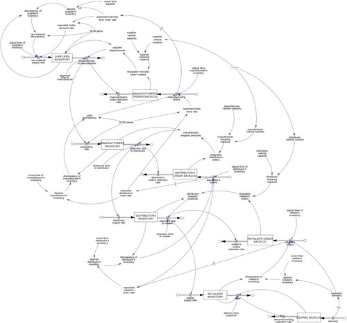
Table 3. Declaration of the used level variables.

Abbreviation	Name	Unit
DB	Demand Backlog	piece
DI	Distributor's Inventory	piece
DOB	Distributor's Order Backlog	piece
MI	Manufacturer's Inventory	piece
MOB	Manufacturer's Order Backlog	part
RI	Retailer's Inventory	piece
ROB	Retailer's Order Backlog	piece
SI	Supplier's Inventory	part

Table 4. Declaration of the used flow variables (excerpt).

Abbreviation	Name	Unit
D	Demand	piece/week
DO	Distributor's Orders	piece/week
MSR	Raw Material Supply Rate	kg/week
MO	Manufacturer's Orders	part/week
RO	Retailer's Orders	piece/week

Table 5. Declaration of the used auxiliary variables (excerpt).

Abbreviation	Name	Unit
DSC	Distributor Shipping Capacity	piece
MSC	Manufacturer Shipping Capacity	piece
SSC	Supplier Shipping Capacity	part

Table 6. Declaration of the used parameter settings (excerpt).

Abbreviation	Name	Value	Unit
BM	BOM Pieces (Manufacturer)	3	part/piece
DVN	Distributor Vehicle Number	25	car
MVN	Manufacturer Vehicle Number	25	car
SVN	Supplier Vehicle Number	25	car

5. Reinforcement learning approach

The use of a system dynamics model as environment makes the use of model-free methods applicable as, in comparison to model-based approaches, the required larger amount of data can be sampled efficiently from the simulation (T. Wang et al. 2019; X. Wang et al. 2022). Taking into account that the system dynamics simulation is already a model for the physical supply chain, model-free algorithms seem to be more suitable in this context to avoid further inaccuracies through approximation. Further advantages of model-free methods are lower computational effort, less tuneable hyperparameters (Moerland et al. 2023), and that they are more straightforward to implement (Zhang and Yu 2020).

Since the inventories of a supply chain are a high-dimensional solution space with a discrete, but very large number of possible states and actions, the assumption of continuous state and action spaces appears to be appropriate, making policy-based methods the preferred choice. Further advantages of this type of algorithms is their better convergence and simpler policy parameterisation (Zhang and Yu 2020).

The next differentiation of RL algorithms can be made whether they are on- or off-policy learners. Off-policy algorithms maintain two different policies, one behaviour policy for data sampling and one target policy that is learned, resulting in higher data efficiency as training samples remain valid over a longer period of time. On-policy algorithms use the same policy for data sampling and learning (X. Wang et al. 2022). As data efficiency is not required with the use of a simulation as environment, in terms of simplicity, on-policy algorithms are the favoured option. For learning a policy in RL, deep neural networks have proven to be suitable general function approximators, also in high dimensional spaces (X. Wang et al. 2022), overcoming a traditional limitation of RL, the curse of dimensionality (Kurian et al. 2022). As recent progress in RL is based on the combination with neural networks (X. Wang et al. 2022), neural networks are selected as framework for approximating the policy function in this work.

Thus, RL algorithms with the outlined properties are applicable for the presented scenario. Specifically, model-free (1) and policy-based (2) methods that are trained on-policy (3) with the help of deep learning (4) are required. A set of possible RL algorithms that fulfils the outlined requirements is presented in Table 7.

Table 7. Comparison of applicable RL algorithms.

		Regularisation		Update measurement		Scaling
Algorithm	Year	Policy update evaluation	Actor-critic	Advantage function	Value function	Asynchrony
PG	1999
PPO	2017	X		X
A2C	2012		X	X
A3C	2016		X	X		X
IMPALA	2018		X		X	X

The policy gradient (PG) algorithm makes use of stochastic gradient descent to update the policy parameters directly (on-policy) based on the estimated gradient of the reward function (Sutton et al. 1999). This basic version of the algorithm suffers from poor data-efficiency and robustness due to improperly sized policy updates (Schulman et al. 2017). In order to achieve more efficient and stable policy updates, regularisation approaches were included into the algorithms to balance the trade-off between exploration and exploitation of the action space. In actor-critic methods this is realised with training a function (the ‘critic’) to adjust the updates of the original policy (the ‘actor’). More specifically, in the advantage actor-critic (A2C) algorithm an estimate for the advantage function is calculated from the maintained value function and then used to scale the policy updates. For a specific action in a given state, this advantage function indicates the difference between the future discounted reward and the state-value (Degris, Pilarski, and Sutton 2012; Mnih et al. 2016). Thus, more intuitively, actor-critic methods scale the policy updates based on how much better a specific action is compared to the average of all actions in a specific state. Out of the actor-critic methods, IMPALA and A3C are designed for asynchronous scaling, which is especially important resource-intensive learning tasks. However, the regarded supply chain model does not require an extensive scaling of computational resources. This motivates the use of A2C, a conceptually simpler approach that has shown to provide competitive performance compared to other actor-critic approaches (Schulman et al. 2017). Nevertheless, for models of real-world supply chains the asynchronous versions of the algorithm may be a valuable approach. In contrast to the actor-critic methods, in PPO the regularisation of policy updates is based on a surrogate expected advantage function, which makes it a conceptually different technique. In order to test different algorithmic approaches for the application on a system dynamics simulation, PPO and A2C were both chosen for experimentation.

The principle of RL builds on the interaction of an agent with an environment. If not declared otherwise, in the experiments the status of all level variables (DB, DI, DOB, MI, MOB, RI, ROB, SI) is reported to the RL agent as observation. High inventory levels in supply chains are associated with costs, therefore it is desirable to fulfil the arising demand $D\left(t\right)$ as accurate as possible. To encourage lean inventories with simultaneous demand fulfilment along the supply chain, the reward function $\mathbf{R}$ is defined as the negative standard deviation from the expected demand ${\mu }_D$. With the tuple of level variable values $L_t=\left(\mathrm{DB}\right(t),\mathrm{DI}(t),\mathrm{DOB}(t),\mathrm{MI}(t),\mathrm{MOB}(t),\mathrm{RI}(t),\mathrm{ROB}(t),\mathrm{SI}(t\left)\right)$ at timestep t, the corresponding reward can be calculated as follows: (2) ${\mathbf{R}}_t=-\sqrt{\sum _{l_t\in L_t}(l_t-{\mu }_D{)}^2}$(2) This function offers the advantage that it represents the optimisation objective more precisely compared to functions that depend directly on the level variables. The relative approach takes into account that a certain level of inventories and backlogs (the expected demand) is unavoidable to meet the customers' demand and therefore not gets penalised. This has shown to prevent the agent from the unintended behaviour of accepting the penalty for a high demand backlog by not passing the orders upstream, as this would increase even more level variables. The supplier's inventory and the manufacturer's order backlog are scaled according to the number of parts per piece before the usage in the reward function. Operational recovery policies are then learned by the RL agent based on the observations of the environment and rewards for the taken actions. 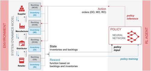As actions the tuples $A_t=\left(\mathrm{DO}\right(t),\mathrm{MO}(t),\mathrm{RO}(t\left)\right)$ are used, indicating the orders from the respective supply chain entities at each timestep t. As policy, a neural network is learned, which takes the observation as input, gives the action as inference output and is trained using the calculated rewards. As environment, an adapted version of the system dynamics model that is presented in Figure 2 was used. Since in the RL approach the model behaviour is controlled by the agent, feedback loops were removed from the system dynamics model and orders are inserted as time-varying parameters. The resulting flow diagram is included in the appendix (Appendix A.3) and the described working principle of the RL integration is summarised in Figure 3.

Figure 3. Visualisation of the RL integration approach.

The system dynamics model is used as RL environment, whose state is sent to the RL agent to learn the and infer from the policy; the resulting action is then transferred back to the environment.

6. Experimental evaluation

In the implementation, the described system dynamics model was transformed into a Python-readable form using the PySD library (Martin-Martinez et al. 2022) and then integrated into a custom gym environment. In this way, the system dynamics simulation can be accessed by the RL-agent. The observation space for each level variable was restricted to $[0,\mathrm{1,000,000}]$ and the action space for orders was restricted to $[0,\mathrm{100,000}]$ each. The restrictions for MO, SI, and MOB were scaled with BM accordingly. For the RL algorithms, the Stable Baselines3 implementation (Raffin et al. 2021) was used. In the implementation, both, action and state values were scaled to continuous values from the interval $[-1,1]$. As trainable policy for PPO and A2C, feed-forward neural networks with unchanged settings from Stable Baselines3 were applied. Hyperparameters that were changed compared to the default settings are indicated in Appendix A.4. All experimental runs were repeated $r=10$ times to mitigate random deviations in the algorithmic performance. The evaluation was executed on a machine with an Intel(R) Core(TM) i7-1065G7 CPU and 16GB RAM in CPU-only mode.

Different types of disruptions are investigated in the experiments, namely disruptions of transport capacities, demand, and supply. In case of simulating a disruption of transport capacities, the parameters DV N, MV N and SV N become time-dependent. $\mathrm{DVN}\left(t\right)$ then can be calculated as (3) $\begin{array}{rl}& \mathrm{DV}{N}_{\mathrm{disrupt}}\left(t\right)\\ & =\{\begin{array}{ll}16,& \mathrm{if}{t}_{\mathrm{disrupt}}<t\le t_{\mathrm{disrupt}}+d_{\mathrm{disrupt}}\\ 25,& \mathrm{otherwise}.\end{array}\end{array}$(3) $\mathrm{MV}{N}_{\mathrm{disrupt}}\left(t\right)$ and $\mathrm{SV}{N}_{\mathrm{disrupt}}\left(t\right)$ are calculated accordingly. As the mentioned parameters vary over time in the disruption scenarios, also the variables indicating the total transport capacities (DSC, MSC, SSC) become time-dependent ($\mathrm{DS}{C}_{\mathrm{disrupt}}\left(t\right)$, $\mathrm{MS}{C}_{\mathrm{disrupt}}\left(t\right)$, $\mathrm{SS}{C}_{\mathrm{disrupt}}\left(t\right)$ ). A disruption of demand $D_{\mathrm{disrupt}}\left(t\right)$ can be calculated as (4) $\begin{array}{rl}& D_{\mathrm{disrupt}}\left(t\right)\\ & =\{\begin{array}{ll}0,& \mathrm{if}{t}_{\mathrm{disrupt}}<t\le t_{\mathrm{disrupt}}+d_{\mathrm{disrupt}}\\ D\left(t\right),& \mathrm{otherwise}\end{array}\end{array}$(4) whereas a disruption of supply can be calculated as (5) $\begin{array}{rl}& \mathrm{MS}{R}_{\mathrm{disrupt}}\left(t\right)\\ & =\{\begin{array}{ll}0,& \mathrm{if}{t}_{\mathrm{disrupt}}<t\le t_{\mathrm{disrupt}}+d_{\mathrm{disrupt}}\\ \mathrm{MSR}\left(t\right),& \mathrm{otherwise}.\end{array}\end{array}$(5) In the experiments, there is a distinction between scenarios with fixed disruptions, in which initiation time and duration are the same in all runs, and scenarios with variable disruptions, in which disruption start and duration are sampled randomly. For the variable disruption scenario, it is assumed that disruptions can not be predicted and therefore that the occurrence of a disruption is equally likely for every timestep. Hence, the variable disruption timing $t_{\mathrm{disrupt},\mathrm{var}}$ is sampled from a uniform distribution (6) $t_{\mathrm{disrupt},\mathrm{var}}\sim \mathcal{U}(t_0,t_n-10),$(6) ensuring that the disruption takes place completely during the observed time period. For the variable duration of disruptions $d_{\mathrm{disrupt},\mathrm{var}}$ , a normal distribution with with mean $\mu =7$ and variance ${\sigma }^2=3$ is assumed: (7) $d_{\mathrm{disrupt},\mathrm{var}}\sim \mathcal{N}(\mu ,{\sigma }^2)$(7) To avoid unintended effects in the implementation, negative disruption durations are set to zero. In case of a fixed disruption, the starting time is set to $t_{\mathrm{disrupt},\mathrm{fix}}=50$ and the duration is set to $d_{\mathrm{disrupt},\mathrm{fix}}=10$.

In total, the proposed approach is tested in three different experimental setups. Experiment 1 serves as a general validation of the RL optimisation under consideration of the given use case from the aerospace and defence industry during the COVID pandemic. This experiment also includes a comparison with the Vensim built-in metaheuristic Powell's method, for which as objective function the stated reward function (Equation 2(2) ${\mathbf{R}}_t=-\sqrt{\sum _{l_t\in L_t}(l_t-{\mu }_D{)}^2}$(2) ) is implemented. In this setup, the general conditions are fixed according to the given use case, this includes a fixed disruption location (transport capacities), a fixed disruption timing and duration (as outlined above), and a fixed demand pattern that is sampled once for all episodes. As in practice disruptions are not predictable, in experiment 2 the algorithmic performance of the proposed RL optimisation approach is investigated under uncertain conditions. The goal is to determine whether it is possible to learn an inventory control policy that is robust against different types of disruptions. The setup of both experiments assumes complete information about inventories and order backlogs along the entire supply chain. Since this is usually not the case in practice, the goal of experiment 3 is to investigate the algorithmic performance under incomplete information. In the Vensim simulation, it is not possible to include changing disruption locations in the optimisation process. Also, Powell's method does not rely on observations, which makes experiment 3 meaningless for this algorithm. For these reasons, only PPO and A2C are compared in experiments 2 and 3. A smoothing function was applied for plotting the experiments to improve the readability of all diagrams.

6.1. Experiment 1 – validation of the RL optimisation on the use case

The objective of experiment 1 (a) is a comparison of the proposed RL optimisation approach with the results of the simulation without optimisation under consideration of the given use case. A comparison with the Vensim built-in metaheuristic Powell's method is carried out in experiment 1 (b). The settings used for the Vensim optimisation are provided in Appendix A.5. In experiment 1 (a), the RL approach as described is used with a sampling of orders at every timestep. The Vensim optimisation only allows the generation of order values that are constant during an episode and act like a parameter in the simulation. To account for this in experiment 1 (b), the environment is modified in a way, that for every simulation run constant orders are generated. The length of an episode is set to five simulation runs and as observation always the initial observation is returned to narrow down the agent on learning only one state-action pair.

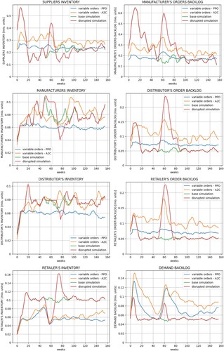
An overview of the results of experiment 1 (a) is provided in Figure 4. The upper diagram shows for both compared algorithms PPO and A2C the mean learning curves of all performed runs including the standard deviation in lighter colours. The lower diagrams compare the inventory and backlog levels summed over all supply chain entities during the simulation interval, indicating the averaged best episode per run. Based on the adopted use case data from Ghadge et al. (2022), these diagrams include simulation results from a disrupted (red lines – disrupted simulation) and a non-disrupted setting (green lines – base simulation). Since both simulations result in partly similar curves, the red lines cover the green lines to some extent. After an initialisation period of about 20 timesteps, the following peak in the curve for the cumulative backlogs results from the fixed disruption occurring from t = 50 until t = 60. The disruption has no effect on the cumulative inventories, even though the inventories of single entities might be affected (see Appendix A.6). In the diagrams, these simulation results are depicted together with the optimisation results of the RL integration (blue lines – PPO, orange lines – A2C). The curves for the aggregated inventories and backlogs show that both algorithms are able to learn undistorted order policies. With regard to the use case, the policies generated by PPO are effective in reducing the variance in inventory and backlog levels caused by the ripple effect of COVID-related disruptions. Additionally, these policies result in lower overall levels of inventory and backlog. Detailed results for all single level variables are presented in Appendix A.6. The learning curves depicted above indicate that, compared to A2C, PPO is leading to better results faster and with less variation. Both algorithms converge in a stable manner without high deviations or performance drops.

Figure 4. Results of experiment 1 (a) – Comparison with the simulation results.

Three diagrams are presented, the first shows the learning curves of both algorithms while the remaining diagrams illustrate the overall levels of inventory and backlogs in the supply chain, also for a simulation setting with and without disruption. The diagrams indicate that PPO delivers the best results for reducing variations in experiment 1 (a).

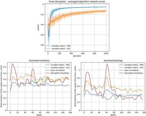
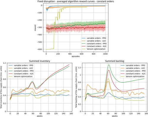
Figure 5 illustrates the results of experiment 1 (b) with a constant order scheme but besides that identical conditions as in (a). As benchmark, also the curves for the proposed stepwise order sampling from experiment 1 (a) are included in the diagrams. The reward curves indicate that stepwise order sampling is more suitable for the RL setting, as both regarded RL algorithms perform significantly better. Powell's method generated the most suitable order policy for the constant order scheme without making use of the maximum number of allowed iterations, since the termination criteria (see Appendix A.5) are met beforehand. In comparison with the stepwise order policy learned by PPO, Powell's method generated a parameter setting with comparable absolute levels of inventory and backlog but with more variation induced by the ripple effect caused by the COVID disruption. Thus, compared to the Vensim built-in metaheuristic optimisation, the proposed RL approach is more suitable to mitigate the ripple effect in the setting adopted from the use case with a fixed disruption. The superior results are caused mainly through the improved flexibility in the stepwise order sampling. However, when comparing Powell's method with the constant orders generated by the RL approach, the metaheuristic results in significantly lower inventory and backlog levels as well as less severe variations.

Figure 5. Results of experiment 1 (b) – Comparison with Powell's method (Vensim optimisation).

Three diagrams are presented, the first shows the learning curves of both algorithms and Powell's method while the remaining diagrams illustrate the overall levels of inventory and backlogs in the supply chain for all regarded settings. The diagrams indicate that PPO with variable orders delivers the best results for reducing variations in experiment 1 (b).

An excerpt of the learned policy is presented in Figure 6. For every timestep, the action learned by the RL algorithm (the order quantity of the distributor) is visualised as blue dot in dependency of the environment. In order to obtain a readable diagram, only the variables indicating the distributor's inventory and the retailer's backlog are included, although the taken action also has a dependency on the remaining level variables. Furthermore, only the learned policy for the distributor is presented. For comparison, the resulting policies of the disrupted simulation (red dots) and the Vensim optimisation (green dots) are included in the diagram as well. Since only the 3D perspective could be misleading, the dependency on each, the distributor's inventory (left diagram) and the retailer's backlog (right diagram) is visualised as well. The plots indicate that the variations in the order quantity are comparable for the RL optimisation and the simulation. Also, the fixed order quantity of the Vensim optimisation is apparent in the diagram. The distribution of the dots indicates that in the simulation, there is a higher variation in the inventory level while for the RL policy, the variation is similar for both level variables. This shows that the objective function, which assigns equal weights to variations in inventory and backlog levels, has the intended balancing effect.

Figure 6. Results of experiment 1 – Visualisation of the learned policy for the distributor.

A diagram visualising the learned policy for the distributor is presented from three perspectives. A 3D chart shows the dependencies between the distributor's orders, the distributor's inventory, and the retailer's backlog. The diagram indicates that the proposed RL integration results in comparable variation in the order quantities.

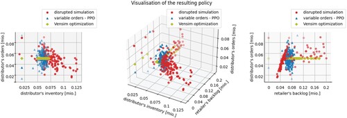
Table 8 shows a comparison of mean computation times of the algorithms. The metaheuristic Powell's method has a significantly lower computation time than the RL algorithms, which are on the same scale with a slight advantage of A2C. During experimentation, it was apparent that the computation times are mainly caused by the interaction with the environment, making this more efficient therefore could speed up the process significantly. Even though, it is unrealistic to reach the metaheuristic computation times due to the computational overhead that RL entails. Thus, the results imply a trade-off between quality of results and computational effort.

Table 8. Comparison of mean computation times for experiment 1 (a).

Algorithm	Mean computation time [sec]
Powell's Method (Vensim)	$<1$
PPO	1006
A2C	958

The overall results from experiment 1 validate that with the proposed RL approach improved order policies can be learned that mitigate the ripple effect induced by the COVID pandemic for a company from the aerospace and defence industry. Out of the tested approaches, stepwise order policies generated by PPO provide the most significant ripple effect mitigation. However, the Vensim built-in metaheuristic Powell's method leads to slightly worse results with significantly less computation time, indicating a trade-off between quality of results and computational effort.

6.2. Experiment 2 – validation of the RL optimisation under uncertainty

In this experiment, the fixed disruption from experiment 1 serves as first scenario but with a demand sampled randomly for every episode. In a second scenario, disruption duration and disruption start are sampled randomly as indicated above. In supply chains, common disruption locations are demand, supply, and logistics capacity (Golan, Jernegan, and Linkov 2020) and it is also not predictable where a disruption occurs. Therefore, in a third scenario, additionally the location of the disruption sampled randomly from the three listed possibilities.

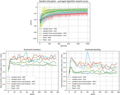
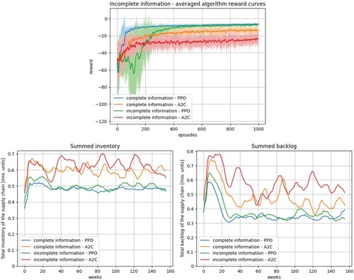
In Figure 7, the results of experiment 2 are summarised, presenting the learning curves, summed inventories, and summed backlogs of the different algorithm-scenario combinations. The missing disruption-related oscillations in the randomised scenarios can be explained by the averaging procedure over all 10 runs. A better performance of PPO can be observed for all three scenarios in the accumulated inventories and backlogs. It can be observed that randomised time characteristics of the disruption do not affect the algorithmic performance negatively while the additional random location slightly increases the variance and absolute value of inventory and backlog levels. The algorithmic performance in the randomised scenarios can be seen as a validation of the RL approach under uncertainty since generalised order policies, independent from a fixed disruption, could be learned. The results from the experiment imply that also if duration, starting time, and location of a disruption are not known beforehand, the proposed approach is able to generate ripple effect-mitigating order policies. Regarding the use case this means that without prior information on the COVID pandemic the reliability of the supply chain can be improved with the combination of system dynamics and RL.

Figure 7. Results of experiment 2 – Validation of the RL optimisation under uncertainty.

Three diagrams are presented, the first shows the learning curves of both algorithms in the different settings while the remaining diagrams illustrate the overall levels of inventory and backlogs in the supply chain for all algorithm-setting combinations. The diagrams indicate that PPO delivers the best results for all settings. Also, uncertainty regarding the time of disruptions almost does not affect the performance while uncertain disruption locations seem to slightly reduce the performance.

6.3. Experiment 3 – validation of the RL optimisation under incomplete information

The effects of incomplete information, which are the subject of this experiment, are investigated under the assumption of time-varying disruptions, generated according to Equations (6(6) $t_{\mathrm{disrupt},\mathrm{var}}\sim \mathcal{U}(t_0,t_n-10),$(6) ) and (7(7) $d_{\mathrm{disrupt},\mathrm{var}}\sim \mathcal{N}(\mu ,{\sigma }^2)$(7) ) and a disruption location fixed to the transport capacities. In this experiment, only the distributor is in scope and the action space is reduced to the distributor's orders accordingly. The remaining orders are covered again by the original simulation. In the first scenario of this experiment, the RL agent can observe all level variables (complete information) whereas in the second scenario, the observation space is reduced to the distributors' inventory, the distributor's backlog, and the retailer's backlog (incomplete information).

For this experiment, the results are presented in Figure 8. Again, PPO leads to lower inventories, lower backlogs, and less variation compared to A2C in both scenarios. The order policies learned by PPO result in almost identical accumulated level of inventories and backlogs in both scenarios, which can be seen as a validation for the applicability of the proposed approach under incomplete information about the state of the supply chain. However, from the learning curve it can be observed that in the beginning of the learning procedure for the scenario with incomplete information it is more difficult for the PPO algorithm to generate suitable order policies. Regarding the use case, this implies that complete information on the supply chain is not mandatory for an effective ripple effect mitigation.

Figure 8. Results of experiment 3 – Validation of the RL optimisation under incomplete information.

Three diagrams are presented, the first shows the learning curves of both algorithms in both settings while the remaining diagrams illustrate the overall levels of inventory and backlogs in the supply chain for all algorithm-setting combinations. The diagrams indicate that PPO delivers the best results for both settings and that incomplete information has no effect on the performance.

7. Discussion

Due to the relevance of supply chain disruptions and their impact on enterprises, there is a need for increased resilience. As disruptions are difficult to predict and the origin typically is located outside the supply chain (Li and Zobel 2020; Llaguno, Mula, and Campuzano-Bolarin 2022), adaptive order policies are an important lever to mitigate the ripple effect at an operational level (Ivanov et al. 2019). The reviewed literature indicates that, in order to address the research gap of SimOpt approaches for ripple effect mitigation through the generation of dynamic recovery policies (Katsaliaki, Galetsi, and Kumar 2022; Liu et al. 2021; Llaguno, Mula, and Campuzano-Bolarin 2022), an RL-based optimisation of system dynamics models is an unexplored but promising field of research. The experimental results show that the proposed approach for creating adaptive order policies is effective in mitigating the ripple effect in a simulation setting.

Experiment 1 demonstrates that an adaptive ordering model based on secondary data from the aerospace and defence industry (Ghadge et al. 2022) can be trained to reduce variations in inventories and order backlogs when disruption characteristics are known. Furthermore, it is shown that an adaptive ordering model trained by the PPO algorithm is more effective in reducing the ripple effect than Powell's method. With this metaheuristic optimisation approach, only an optimised constant value for the orders can be generated. When restricting the RL algorithms also to the generation of a constant order value, the metaheuristic approach shows a significantly better performance, indicating that the superior results of PPO are related to the possibility of stepwise changes in the order quantity. Experiment 2 proves that RL is also effective for learning adaptive order policies when disruption characteristics are not known beforehand. Since the occurrence and properties of real-world disruptions are not predictable (Dolgui, Ivanov, and Sokolov 2018), this represents a more realistic setting. In both experiments, the RL agent is trained with information about inventories and order backlogs from all supply chain entities. Since this complete information is an assumption that usually does not hold in practice, experiment 3 showcases the effectiveness of the proposed approach also in a setting with incomplete information about inventories and backlogs along the supply chain. The plots of the resulting policy from the RL optimisation (Figure 6) allow for a comparison with traditional heuristic inventory policies. For example, an (s, Q) policy, where below inventory level s, an order with a fixed quantity Q is placed (El-Aal et al. 2010), would result in a pattern similar to the Vensim simulation. Since traditional inventory policies are only dependent on the current inventory level (El-Aal et al. 2010), neglecting the informative value of order backlogs, a higher variation in the backlog levels is to be expected. A detailed comparison with different traditional inventory policies is subject to further research, but as shown by Kegenbekov and Jackson (2021), an optimisation with RL is more effective in streamlining inventor management than a traditional base-stock policy.

Since the proposed combination of system dynamics and RL works in a simulation environment, a continuous validation of the learned order policies should be performed when using the approach in real conditions. If a model does not reflect the reality and influencing factors are not considered, the generated order policies are likely to be inaccurate as well. Furthermore, the scaling properties of the approach to large supply chains have not been not tested.

8. Managerial insights and theoretical implications

An implication from a practical and managerial perspective to mitigate the costly consequences of the ripple effect like shortages and excess inventories is the integration of an algorithmic ordering approach into a general supply chain resilience framework. As preventive recovery policy, classical heuristic inventory control policies could be substituted by the proposed combination of system dynamics and RL, which has shown to effectively balance inventories and order backlogs, even under practice-oriented conditions such as uncertainty about disruption characteristics and incomplete information about the supply chain. Based on the SimOpt approach, robust order policies can be generated without information on time, duration, and location of the disruption and tedious scenario building as necessary for simulation-only approaches can be avoided. In comparison to proactive mitigation approaches or structural adaptations of the supply chain, the algorithmic generation of recovery policies with a SimOpt approach is also a cost-effective option to build resilience. Thus, the combination of system dynamics and RL appears to be a promising approach that requires a practical evaluation. As additional managerial implication, the SimOpt approach could be used as part of the mathematical engine of a digital twin for supply chains. Managerial supply chain decision-makers can be supported in mitigating the ripple effect through improved visibility on the supply chain behaviour under disruptions. A digital twin allows for the evaluation of a multitude of different resilience-building measures such as backup suppliers or alternative shipping routes. Moreover, the creation of a digital twin would require information sharing and the collaboration of multiple supply chain echelons, which has synergies with the proactive ripple effect mitigation approach.

An implication from a theoretical and research perspective is the extension of the set of SimOpt-based approaches for SCM as well as the advance of research in supply chain resilience. Based on existing research on system dynamics simulations supply chain disruptions, the effectiveness of the integration of RL for ripple effect mitigation has been demonstrated in comparison to a pure simulation and a metaheuristic for a use case from the aerospace and defence industry. From a theoretical viewpoint, the approach combines the computational efficiency and robustness of system dynamics simulations (Jaenichen et al. 2021) with the suitability of RL for solving dynamic optimisation problems (Mortazavi, Khamseh, and Azimi 2015). Furthermore, the approach allows to learn robust order policies without the need for historical data, which is difficult to obtain for supply chain disruptions. RL approaches for inventory optimisation usually refer to the inventory management model from the OR-Gym package as environment that supports single product systems with stationary demand (Hubbs et al. 2020). Hence, the proposed approach of using a system dynamics simulation as environment allows a flexible adaption to different supply chain configurations, i.e. multi-product or seasonal demand, using a graphical representation of the model as well as the opportunity to integrate a variety of different disruptions to test the system under varying conditions. Here, this proposal can be seen as a foundation for future research, as it presents a flexible optimisation approach that is applicable to a wide range of supply chain-related problems.

9. Conclusions and future research

Due to the significant impact of supply chain disruptions on companies' operations, resilience is an inevitable requirement for competitiveness. Resilience can be increased on an operational level through adaptive order policies for recovery, which can be generated by algorithmic approaches. Since a research gap exists regarding the development of SimOpt approaches for the generation of these recovery policies, a novel framework that integrates system dynamics and RL is proposed for the generation of adaptive order policies. For this purpose, (i) a system dynamics model is derived from the literature that allows for the simulation of all types of disruptions based on secondary data from a real use case. In addition, (ii) the proposed approach is presented, in which the supply chain behaviour is simulated with the system dynamics model and adaptive order policies for improved disruption recovery are learned by the RL agent. The effectiveness of the approach is demonstrated in an experimental setting (iii). The results indicate that the general working principle of the proposed optimisation approach is promising since the proposed combination of a system dynamics simulation with RL has shown to be robust also with uncertainty about the disruption characteristics and under incomplete information about the state of the supply chain. The proposed approach is a versatile framework that allows a flexible and straightforward adaptation to changing supply chain configurations. In all experimental runs, PPO outperformed A2C regarding the quality of results, even though A2C had slightly lower computation times.

A limitation of this study relates to the comparison with alternative ripple effect mitigation approaches with, e.g. backup suppliers or alternative shipping routes. This would provide the ability to assess the effectiveness as well as the financial and organisational efforts of the different methods, allowing a derivation of guidelines for preferable mitigation approaches depending on the disruption characteristics and supply chain configuration. Related to this, a comparison with traditional order policies could provide additional insights about the effectiveness of the system dynamics-RL framework for ripple effect mitigation. Another major limitation for the presented approach is that the generated order policies were not evaluated in practice. By using the learned order policies in a real-world supply chain setting, the effectiveness and practicality can be evaluated. This may lead to valuable improvements and allows conclusions regarding the applicability of the approach and an identification of optimisation potential. In addition, models are always a bounded representation of reality, limiting the range of conclusions that can be drawn from the results, in particular for special cases of disruptions. Also, the used system dynamics model only represents a small supply chain. Usually multiple entities per echelon exist and multiple products are in scope of a similar analysis. Another limitation is that, despite trial runs during the implementation, different reward functions were not tested systematically. The experiments indicate that the used reward function depending on the variance is able to balance the level variables under disruptions but the objective of minimum inventories and backlogs is not directly addressed, which could further improve the results. During experimentation, the model has shown to be very sensitive for changes on the hyperparameter settings. The use of a systematic approach to optimise the hyperparameter settings and the configuration of the underlying neural network is likely to lead to more precise order policies and would also enable a structured testing of different reward functions. Despite a justified selection of algorithms, further RL approached that were not tested in this work may increase the performance.

Since the proposed integration of system dynamics and RL represents a novel approach for ripple effect mitigation, several possible directions for future research exist. With regard to supply chain resilience, in general, additional research is needed to combine existing proactive and reactive measures with the system dynamics-RL framework to achieve redundancy in ripple effect mitigation. Alternative approaches are the integration of these measures, e.g. backup suppliers, into the model or the inclusion of the system dynamics-RL approach in other frameworks with the aim to increase supply chain resilience. Furthermore, a benchmark with other algorithmic approaches might be beneficial where alternative simulation or optimisation techniques can be tested and assessed regarding their applicability in the given setting. Additional activities are required regarding the application of the proposed approach in practice. For a successful application on a real-world supply chain a precise model of the supply chain is inevitable for obtaining useful results. In this context, further investigations might be necessary to refine the approach. Current trends regarding sustainability may be also considered and the effects on a closed-loop supply chain (e.g. Gu and Gao 2017) can be tested in future research. As shown in Figure 6, the resulting policies could be investigated systematically in future research, especially in comaprison to traditional order policies. The problem of incomplete information about the supply chain, which was investigated in experiment 3, may be addressed by research on federated learning, which provides the potential to enhance the willingness for and security of data sharing along the supply chain. In this context, also further collaborative approaches like joint coordination and decision-making can be explored to mitigate the ripple effect more effectively. A further line of investigation can be related to the design of effective reward functions, tailored towards the problem of minimal inventories and backlogs for all supply chain entities. Approaches from multi-objective RL (e.g. Hayes et al. 2022) can be suitable to design a reward function that addresses all level variables independently and thus avoids the dependency on the estimated demand. In contrast to the applied reward function that relies only on inventory and backlog levels, further approaches may focus on optimising costs of inventories and backlogs, service levels, or lead time. Future algorithmic research may be related to multi-agent approaches (see, e.g. H. Wang et al. 2022), which provide the potential to represent real-world supply chain behaviour more closely.

Disclosure statement

No potential conflict of interest was reported by the author(s).

Data availability statement

The authors confirm that the data supporting the findings of this study are available within the article and its supplementary materials. The source code leading to the findings of this study is available from the corresponding author upon request.

Additional information

Funding

The research leading to these results received funding from the project ‘Industrial Production and Logistics Optimization in Industry 4.0’ (i4OPT) (Ref. PROMETEO/2021/065) granted by the Valencian Regional Government; and the grant PDC2022-133957-I00 funded by the Spanish Ministry of Science, Innovation and Universities (MCIN/AEI /10.13039/501100011033) as part of the European Union Next Generation EU/RTRP programme.

Notes on contributors

Fabian Bussieweke

Fabian Bussieweke graduated with an M.Sc. in Business Administration and Engineering: Mechanical Engineering from RWTH Aachen University, Germany and with a Master's degree in Advanced Engineering in Production, Logistics and Supply Chain from the Universitat Politècnica de València (UPV), Spain. Currently, he is a Ph.D. student at the Technical University of Munich, Germany. His main research interests are the application of operations research and machine learning to production, logistics and supply chain management, including modelling and simulation in these areas.

Josefa Mula

Josefa Mula is Professor in the Department of Business Management of the Universitat Politècnica de València (UPV), Spain. She is a member of the Research Centre on Production Management and Engineering (CIGIP) of the UPV. Her teaching and principal research interests concern production management and engineering, operations research and supply chain simulation. She is editor in chief of the International Journal of Production Management and Engineering. She regularly acts as associate editor, guest editor and member of scientific boards of international journals and conferences, and as referee for more than 50 scientific journals. She is author of more than 140 papers mostly published in international books and high-quality journals, among which International Journal of Production Research, Fuzzy sets and Systems, Production Planning and Control, International Journal of Production Economics, European Journal of Operational Research, Computers and Industrial Engineering, Journal of Manufacturing Systems and Journal of Cleaner Production.

Francisco Campuzano-Bolarin

Francisco Campuzano-Bolarín is Professor in the Business Management Department at the Technical University of Cartagena (UPCT) in Spain. Having graduated in 2000 in Management Engineering, in 2006 he received a Ph.D. degree in Management from the Universitat Politècnica de València. His doctoral thesis was rewarded with honours by the Spanish Logistics Centre (CEL) in 2007. His main fields of research are focused on the modeling and simulation of supply chain systems and production management using the system dynamics methodology. He has participated in 19 research projects of public competition at regional, national and international level, and 12 research contracts with public and private entities. He is author of more than 40 publications published in scientific international peer reviewed journals included in JCR. Author of one book and three book chapters, both in international editorials (Springer and Pearson). He has also contributed to several international conference proceedings. He is currently an active member of the Systems Dynamic Society. He is a reviewer for several high-quality international journals and member of scientific boards of international journals.

Appendix. Additional Vensim implementation details

A.1. Variable declarations

In the following, all used variables are declared together with their respective unit. For completeness, also the variables introduced in the main text are included.

Table A1. Declaration of the used level variables.

Abbreviation	Name	Unit
DB	Demand Backlog	piece
DI	Distributor's Inventory	piece
DOB	Distributor's Order Backlog	piece
MI	Manufacturer's Inventory	piece
MOB	Manufacturer's Order Backlog	part
RI	Retailer's Inventory	piece
ROB	Retailer's Order Backlog	piece
SI	Supplier's Inventory	part

Table A2. Declaration of the used flow variables.

Abbreviation	Name	Unit
D	Demand	piece/week
DBR	Demand Backlog Reduction Rate	piece/week
DO	Distributor's Orders	piece/week
DOR	Distributor's Order Reduction Rate	piece/week
DSR	Distributor Supply Rate	piece/week
MSR	Raw Material Supply Rate	kg/week
MO	Manufacturer's Orders	part/week
MOR	Manufacturer's Order Reduction Rate	part/week
PR	Production Rate	piece/week
RO	Retailer's Orders	piece/week
ROR	Retailer's Orders Reduction Rate	piece/week
RSR	Retailer Supply Rate	piece/week
S	Sales	piece/week
SRD	Shipment Rate to Distributor	piece/week
SRM	Shipment Rate to Manufacturer	part/week
SRR	Shipment Rate to Retailer	piece/week

Table A3. Declaration of the used auxiliary variables.

Abbreviation	Name	Unit
DID	Discrepancy of Distributor's Inventory	part
DIS	Discrepancy of Supplier's Inventory	part
DIR	Discrepancy of Retailer's Inventory	piece
DIM	Discrepancy of Manufacturer's Inventory	piece
DDI	Desired Distributor's Inventory	piece
DMI	Desired Manufacturer's Inventory	piece
DRI	Desired Retailer's Inventory	piece
DSC	Distributor Shipping Capacity	piece
DSI	Desired Supplier's Inventory	part
DSP	Distributor Shipped Products	piece
ED	Expected Demand	piece/week
EDO	Expected Distributor's Order Rate	piece/week
EMN	Expected Material Need Rate	kg/week
EMO	Expected Manufacturer's Order Rate	part/week
EPN	Expected Parts Need Rate	part/week
ERO	Expected Retailer's Order Rate	piece/week
MD	Raw Material Discrepancy	kg
MSC	Manufacturer Shipping Capacity	piece
MSP	Manufacturer Shipped Products	piece
PD	Parts Discrepancy	part
SDO	Shippable Distributor's Orders	piece
SMO	Shippable Manufacturer's Orders	part
SRO	Shippable Retailer's Orders	piece
SSC	Supplier Shipping Capacity	part
SSP	Supplier Shipped Parts	part

Table A4. Declaration of the used parameter settings.

Abbreviation	Name	Value	Unit
AD	Adjust Time Distributor's Inventory	5	week
AM	Adjust Time Manufacturer's Inventory	5	week
AR	Adjust Time Retailer's Inventory	5	week
AS	Adjust Time Supplier's Inventory	5	week
BS	BOM Parts (Supplier)	12	kg/part
BM	BOM Pieces (Manufacturer)	3	part/piece
CD	Cover Time Distributor	1.5	week
CS	Cover Time Supplier	1.5	week
CM	Cover Time Manufacturer	1.5	week
CR	Cover Time Retailer	2	week
DT	Delivery Time to Customer	1	week
DVC	Distributor Vehicle Capacity	2500	piece/car
DVN	Distributor Vehicle Number	25	car
MVC	Manufacturer Vehicle Capacity	2500	piece/car
MVN	Manufacturer Vehicle Number	25	car
SD	Shipment Time to Distributor	1	week
SM	Shipment Time to Manufacturer	1	week
SR	Shipment Time to Retailer	1	week
SVC	Supplier Vehicle Capacity	7500	part/car
SVN	Supplier Vehicle Number	25	car

A.2. Model formulas

The dynamic relations between the variables are indicated by Equations (A1(A1) $\begin{array}{rl}\mathrm{DB}\left(t\right)& ={\int }_{t_0}^{t}D\left(t\right)-\mathrm{DBR}\left(t\right)\mathrm{d}t;\mathrm{DB}\left(t_0\right)=0\end{array}$(A1) )–(A49(A49) $\begin{array}{rl}\mathrm{SSP}\left(t\right)& =min\left\{\mathrm{SI}\right(t),\mathrm{SMO}(t\left)\right\}\end{array}$(A49) ). Equations (A1(A1) $\begin{array}{rl}\mathrm{DB}\left(t\right)& ={\int }_{t_0}^{t}D\left(t\right)-\mathrm{DBR}\left(t\right)\mathrm{d}t;\mathrm{DB}\left(t_0\right)=0\end{array}$(A1) )–(A8(A8) $\begin{array}{rl}\mathrm{SI}\left(t\right)& ={\int }_{t_0}^t\frac{\mathrm{MSR}\left(t\right)}{\mathrm{BS}}-\mathrm{SRM}\left(t\right)\mathrm{d}t;\mathrm{SI}\left(t_0\right)=\mathrm{60,000}\end{array}$(A8) ) determine the behaviour of the level variables. They result from the integral of incoming and outgoing flow determined by the state of the flow variables. With exception of the supplier inventory $\mathrm{SI}\left(t\right)$ (Equation (A8(A8) $\begin{array}{rl}\mathrm{SI}\left(t\right)& ={\int }_{t_0}^t\frac{\mathrm{MSR}\left(t\right)}{\mathrm{BS}}-\mathrm{SRM}\left(t\right)\mathrm{d}t;\mathrm{SI}\left(t_0\right)=\mathrm{60,000}\end{array}$(A8) )), all level variables have an initial value 10,000. Considering the composition of one piece out of three parts (indicated by BM), the supplier inventory $\mathrm{SI}\left(t\right)$ was set to 30,000 as initial value ensure a demand coverage comparable to the other inventories. The flow variables, that are fully determined by the system, are indicated by Equations (A9(A9) $D\left(t\right)\sim \mathcal{N}(\mu ,{\sigma }^2);D\left(t_0\right)=0$(A9) )–(A24(A24) $\begin{array}{rl}\mathrm{SRR}\left(t\right)& =\frac{\mathrm{DSP}\left(t\right)}{\mathrm{SR}}\end{array}$(A24) ). The demand $D\left(t\right)$ is sampled randomly for every timestep from a normal distribution (Equation (A9(A9) $D\left(t\right)\sim \mathcal{N}(\mu ,{\sigma }^2);D\left(t_0\right)=0$(A9) )). The behaviour of the auxiliary variables is defined by Equations (A25(A25) $\begin{array}{rl}\mathrm{DID}\left(t\right)& =\mathrm{DDI}\left(t\right)-\mathrm{DI}\left(t\right)\end{array}$(A25) ) –(A49(A49) $\begin{array}{rl}\mathrm{SSP}\left(t\right)& =min\left\{\mathrm{SI}\right(t),\mathrm{SMO}(t\left)\right\}\end{array}$(A49) ), of which the equations for expected demand ($\mathrm{ED}\left(t\right)$), expected distributor's orders ($\mathrm{EDO}\left(t\right)$), expected manufacturer's orders ($\mathrm{EMO}\left(t\right)$), and expected retailer's orders ($\mathrm{ERO}\left(t\right)$) describe an information delay of one period until they receive the states from their associated flow variables. Accordingly, the simulation is initialised in period t = 0 with the values indicated by the formulas and starts in period t = 1.

Level variables: (A1) $\begin{array}{rl}\mathrm{DB}\left(t\right)& ={\int }_{t_0}^{t}D\left(t\right)-\mathrm{DBR}\left(t\right)\mathrm{d}t;\mathrm{DB}\left(t_0\right)=0\end{array}$(A1) (A2) $\begin{array}{rl}\mathrm{DI}\left(t\right)& ={\int }_{t_0}^t\mathrm{DSR}\left(t\right)-\mathrm{SRR}\left(t\right)\mathrm{d}t;\mathrm{DI}\left(t_0\right)=\mathrm{20,000}\end{array}$(A2) (A3) $\begin{array}{rl}\mathrm{DOB}\left(t\right)& ={\int }_{t_0}^t\mathrm{DO}\left(t\right)-\mathrm{DOR}\left(t\right)\mathrm{d}t;\mathrm{DOB}\left(t_0\right)=0\end{array}$(A3) (A4) $\begin{array}{rl}\mathrm{MI}\left(t\right)& ={\int }_{t_0}^t\mathrm{PR}\left(t\right)-\mathrm{SRD}\left(t\right)\mathrm{d}t;\mathrm{MI}\left(t_0\right)=\mathrm{20,000}\end{array}$(A4) (A5) $\begin{array}{rl}\mathrm{MOB}\left(t\right)& ={\int }_{t_0}^t\mathrm{MO}\left(t\right)-\mathrm{MOR}\left(t\right)\mathrm{d}t;\mathrm{MOB}\left(t_0\right)=0\end{array}$(A5) (A6) $\begin{array}{rl}\mathrm{RI}\left(t\right)& ={\int }_{t_0}^t\mathrm{RSR}\left(t\right)-S\left(t\right)\mathrm{d}t;\mathrm{RI}\left(t_0\right)=\mathrm{20,000}\end{array}$(A6) (A7) $\begin{array}{rl}\mathrm{ROB}\left(t\right)& ={\int }_{t_0}^t\mathrm{RO}\left(t\right)-\mathrm{ROR}\left(t\right)\mathrm{d}t;\mathrm{ROB}\left(t_0\right)=0\end{array}$(A7) (A8) $\begin{array}{rl}\mathrm{SI}\left(t\right)& ={\int }_{t_0}^t\frac{\mathrm{MSR}\left(t\right)}{\mathrm{BS}}-\mathrm{SRM}\left(t\right)\mathrm{d}t;\mathrm{SI}\left(t_0\right)=\mathrm{60,000}\end{array}$(A8) Flow variables:

For comprehensiveness, the demand $D\left(t\right)$ is normally distributed with mean $\mu =\mathrm{50,000}$ and variance ${\sigma }^2=5000$: (A9) $D\left(t\right)\sim \mathcal{N}(\mu ,{\sigma }^2);D\left(t_0\right)=0$(A9) The rest of the flow variables is defined as follows: (A10) $\begin{array}{rl}\mathrm{DBR}\left(t\right)& =S\left(t\right)\end{array}$(A10) (A11) $\begin{array}{rl}\mathrm{DO}\left(t\right)& =max\left\{\mathrm{ERO}\right(t)+\frac{\mathrm{DID}\left(t\right)}{\mathrm{AD}},0\};\mathrm{DO}\left(t_0\right)=0\end{array}$(A11) (A12) $\begin{array}{rl}\mathrm{DOR}\left(t\right)& =\mathrm{SRD}\left(t\right)\end{array}$(A12) (A13) $\begin{array}{rl}\mathrm{DSR}\left(t\right)& =\mathrm{SRD}\left(t\right)\end{array}$(A13) (A14) $\begin{array}{rl}\mathrm{MSR}\left(t\right)& =max\left\{\mathrm{EMN}\right(t)+\frac{\mathrm{MD}\left(t\right)}{\mathrm{AS}},0\}\end{array}$(A14) (A15) $\begin{array}{rl}\mathrm{MO}\left(t\right)& =max\left\{\mathrm{EPN}\right(t)+\frac{\mathrm{PD}\left(t\right)}{\mathrm{AM}},0\};\mathrm{MO}\left(t_0\right)=0\end{array}$(A15) (A16) $\begin{array}{rl}\mathrm{MOR}\left(t\right)& =\mathrm{SRM}\left(t\right)\end{array}$(A16) (A17) $\begin{array}{rl}\mathrm{PR}\left(t\right)& =\frac{\mathrm{SRM}\left(t\right)}{\mathrm{BM}}\end{array}$(A17) (A18) $\begin{array}{rl}\mathrm{RO}\left(t\right)& =max\left\{\mathrm{ED}\right(t)+\frac{\mathrm{DIR}\left(t\right)}{\mathrm{AR}},0\};\mathrm{RO}\left(t_0\right)=0\end{array}$(A18) (A19) $\begin{array}{rl}\mathrm{ROR}\left(t\right)& =\mathrm{SRR}\left(t\right)\end{array}$(A19) (A20) $\begin{array}{rl}\mathrm{RSR}\left(t\right)& =\mathrm{SRR}\left(t\right)\end{array}$(A20) (A21) $\begin{array}{rl}S\left(t\right)& =\frac{min\left\{\mathrm{DB}\right(t),\mathrm{RI}(t\left)\right\}}{\mathrm{DT}}\end{array}$(A21) (A22) $\begin{array}{rl}\mathrm{SRD}\left(t\right)& =\frac{\mathrm{MSP}\left(t\right)}{\mathrm{SD}}\end{array}$(A22) (A23) $\begin{array}{rl}\mathrm{SRM}\left(t\right)& =\frac{\mathrm{SSP}\left(t\right)}{\mathrm{SM}}\end{array}$(A23) (A24) $\begin{array}{rl}\mathrm{SRR}\left(t\right)& =\frac{\mathrm{DSP}\left(t\right)}{\mathrm{SR}}\end{array}$(A24) Auxiliary variables: (A25) $\begin{array}{rl}\mathrm{DID}\left(t\right)& =\mathrm{DDI}\left(t\right)-\mathrm{DI}\left(t\right)\end{array}$(A25) (A26) $\begin{array}{rl}\mathrm{DIS}\left(t\right)& =\mathrm{DSI}\left(t\right)-\mathrm{SI}\left(t\right)\end{array}$(A26) (A27) $\begin{array}{rl}\mathrm{DIR}\left(t\right)& =max\left\{\mathrm{DRI}\right(t)-\mathrm{RI}(t),0\}\end{array}$(A27) (A28) $\begin{array}{rl}\mathrm{DIM}\left(t\right)& =\mathrm{DMI}\left(t\right)-\mathrm{MI}\left(t\right)\end{array}$(A28) (A29) $\begin{array}{rl}\mathrm{DDI}\left(t\right)& =\mathrm{ERO}\left(t\right)\ast \mathrm{CD}\end{array}$(A29) (A30) $\begin{array}{rl}\mathrm{DMI}\left(t\right)& =\mathrm{EDO}\left(t\right)\ast \mathrm{CM}\end{array}$(A30) (A31) $\begin{array}{rl}\mathrm{DRI}\left(t\right)& =\mathrm{ED}\left(t\right)\ast \mathrm{CR}\end{array}$(A31) (A32) $\begin{array}{rl}\mathrm{DSC}& =\mathrm{DVC}\ast \mathrm{DVN}\end{array}$(A32) (A33) $\begin{array}{rl}\mathrm{DSI}\left(t\right)& =\mathrm{EMO}\left(t\right)\ast \mathrm{CS}\end{array}$(A33) (A34) $\begin{array}{rl}\mathrm{DSP}\left(t\right)& =min\left\{\mathrm{DI}\right(t),\mathrm{SRO}(t\left)\right\}\end{array}$(A34) (A35) $\begin{array}{rl}\mathrm{ED}\left(t\right)& =D(t-1)\end{array}$(A35) (A36) $\begin{array}{rl}\mathrm{EDO}\left(t\right)& =\mathrm{DO}(t-1)\end{array}$(A36) (A37) $\begin{array}{rl}\mathrm{EMN}\left(t\right)& =\mathrm{EMO}\left(t\right)\ast \mathrm{BM}\end{array}$(A37) (A38) $\begin{array}{rl}\mathrm{EMO}\left(t\right)& =\mathrm{MO}(t-1)\end{array}$(A38) (A39) $\begin{array}{rl}\mathrm{EPN}\left(t\right)& =\mathrm{EDO}\left(t\right)\ast \mathrm{BM}\end{array}$(A39) (A40) $\begin{array}{rl}\mathrm{ERO}\left(t\right)& =\mathrm{RO}(t-1)\end{array}$(A40) (A41) $\begin{array}{rl}\mathrm{MD}\left(t\right)& =\mathrm{DIS}\left(t\right)\ast \mathrm{BS}\end{array}$(A41) (A42) $\begin{array}{rl}\mathrm{MSC}& =\mathrm{MVC}\ast \mathrm{MVN}\end{array}$(A42) (A43) $\begin{array}{rl}\mathrm{MSP}\left(t\right)& =min\left\{\mathrm{MI}\right(t),\mathrm{SDO}(t\left)\right\}\end{array}$(A43) (A44) $\begin{array}{rl}\mathrm{PD}\left(t\right)& =\mathrm{DIM}\left(t\right)\ast \mathrm{BM}\end{array}$(A44) (A45) $\begin{array}{rl}\mathrm{SDO}\left(t\right)& =min\left\{\mathrm{MSC}\right(t),\mathrm{DOB}(t\left)\right\}\end{array}$(A45) (A46) $\begin{array}{rl}\mathrm{SMO}\left(t\right)& =min\left\{\mathrm{SSC}\right(t),\mathrm{MOB}(t\left)\right\}\end{array}$(A46) (A47) $\begin{array}{rl}\mathrm{SRO}\left(t\right)& =min\left\{\mathrm{DSC}\right(t),\mathrm{ROB}(t\left)\right\}\end{array}$(A47) (A48) $\begin{array}{rl}\mathrm{SSC}& =\mathrm{SVC}\ast \mathrm{SVN}\end{array}$(A48) (A49) $\begin{array}{rl}\mathrm{SSP}\left(t\right)& =min\left\{\mathrm{SI}\right(t),\mathrm{SMO}(t\left)\right\}\end{array}$(A49)

A.3. Model used in optimisation approach

Figure A1. Flow diagram of the supply chain model without feedback loops used for optimisation.

The presented reduced supply chain model again includes four echelons with one entity each, namely the supplier, the manufacturer, the distributor, and the retailer. The feedback loops are removed to enable their substitution through the RL agent.

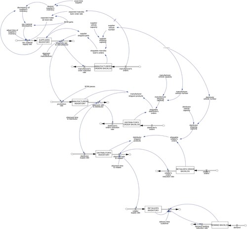
A.4. RL hyperparameter settings

Hyperparameters deviating from the default settings are set as follows in the optimisation. The batch size was set to b = 156, corresponding to the episode length, which is in turn representing the regarded time period of 156 weeks. The discount factor was set to $\gamma =0.9$. In each experimental run, the respective RL algorithm was trained for I = 1000 episodes and the results of the episode with the highest cumulative reward was saved for later evaluation. As learning rate α, an adaptive schedule with i indicating the current episode number was used: (A50) ${\alpha }_i=0.0003\ast {\mathrm{e}}^{\frac{I-i}{I}-1}$(A50)

A.5. Vensim optimisation settings

In the experiments, the following settings for the Vensim optimisation were used:

A.6. Experiment 1 (a) – level variables diagrams

Figure A2. Detailed inventory and backlog curves for experiment 1 (a).

Eight diagrams are presented, the progression of the level variables over time for both algorithms as well as for a disrupted and a non-disrupted simulation setting.

References

- Alves, J. C., and G. R. Mateus. 2022. “Multi-Echelon Supply Chains with Uncertain Seasonal Demands and Lead Times Using Deep Reinforcement Learning.” arXiv preprint arXiv:2201.04651.
- Aslam, T., and A. H. C. Ng. 2016. “Combining System Dynamics and Multi-Objective Optimization with Design Space Reduction.” Industrial Management & Data Systems 116 (2): 291–321. https://doi.org/10.1108/IMDS-05-2015-0215.
- Bottani, E., and R. Montanari. 2010. “Supply Chain Design and Cost Analysis Through Simulation.” International Journal of Production Research 48 (10): 2859–2886. https://doi.org/10.1080/00207540902960299.
- Campuzano, F., and J. Mula. 2011. Supply Chain Simulation: A System Dynamics Approach for Improving Performance. London, Dordrecht, Heidelberg, New York: Springer Science & Business Media.
- Degris, T., P. M. Pilarski, and R. S. Sutton. 2012. “Model-Free Reinforcement Learning with Continuous Action in Practice.” In 2012 American Control Conference (ACC), 2177–2182. IEEE.
- Dolgui, A., D. Ivanov, and B. Sokolov. 2018. “Ripple Effect in the Supply Chain: An Analysis and Recent Literature.” International Journal of Production Research 56 (1–2): 414–430. https://doi.org/10.1080/00207543.2017.1387680.
- El-Aal, A., M. A. El-Sharief, A. E. El-Deen, and A.-B. Nassr. 2010. “A Framework for Evaluating and Comparing Inventory Control Policies in Supply Chains.” JES. Journal of Engineering Sciences 38 (2): 449–465. https://doi.org/10.21608/jesaun.2010.124377.
- Esteso, A., D. Peidro, J. Mula, and M. Díaz-Madroñero. 2023. “Reinforcement Learning Applied to Production Planning and Control.” International Journal of Production Research 61 (16): 5772–5789. https://doi.org/10.1080/00207543.2022.2104180.
- Gadewadikar, J., and J. Marshall. 2023. “A Methodology for Parameter Estimation in System Dynamics Models Using Artificial Intelligence.” Systems Engineering 27 (2): 253–266.
- Ghadge, A., M. Er, D. Ivanov, and A. Chaudhuri. 2022. “Visualisation of Ripple Effect in Supply Chains Under Long-Term, Simultaneous Disruptions: A System Dynamics Approach.” International Journal of Production Research 60 (20): 6173–6186. https://doi.org/10.1080/00207543.2021.1987547.
- Golan, M. S., L. H. Jernegan, and I. Linkov. 2020. “Trends and Applications of Resilience Analytics in Supply Chain Modeling: Systematic Literature Review in the Context of the Covid-19 Pandemic.” Environment Systems and Decisions 40 (2): 222–243. https://doi.org/10.1007/s10669-020-09777-w.
- Gu, Q., and T. Gao. 2017. “Production Disruption Management for R/m Integrated Supply Chain Using System Dynamics Methodology.” International Journal of Sustainable Engineering 10 (1): 44–57. https://doi.org/10.1080/19397038.2016.1250838.
- Hayes, C. F., R. Rădulescu, E. Bargiacchi, J. Källström, M. Macfarlane, M. Reymond, T. Verstraeten, et al. 2022. “A Practical Guide to Multi-Objective Reinforcement Learning and Planning.” Autonomous Agents and Multi-Agent Systems 36 (1): 26. https://doi.org/10.1007/s10458-022-09552-y.
- Heidary, M. H., and A. Aghaie. 2019. “Risk Averse Sourcing in a Stochastic Supply Chain: A Simulation-Optimization Approach.” Computers & Industrial Engineering 130:62–74. https://doi.org/10.1016/j.cie.2019.02.023.
- Hubbs, C. D., H. D. Perez, O. Sarwar, N. V. Sahinidis, I. E. Grossmann, and J. M. Wassick. 2020. “Or-Gym: A Reinforcement Learning Library for Operations Research Problems.” arXiv preprint arXiv:2008.06319.
- Ivanov, D. 2017. “Simulation-Based Ripple Effect Modelling in the Supply Chain.” International Journal of Production Research 55 (7): 2083–2101. https://doi.org/10.1080/00207543.2016.1275873.
- Ivanov, D. 2019. “Disruption Tails and Revival Policies: A Simulation Analysis of Supply Chain Design and Production-Ordering Systems in the Recovery and Post-Disruption Periods.” Computers & Industrial Engineering 127:558–570. https://doi.org/10.1016/j.cie.2018.10.043.
- Ivanov, D., A. Dolgui, A. Das, and B. Sokolov. 2019. “Digital Supply Chain Twins: Managing the Ripple Effect, Resilience, and Disruption Risks by Data-Driven Optimization, Simulation, and Visibility.” In Handbook of Ripple Effects in the Supply Chain, 309–332. Cham, Switzerland: Springer.
- Ivanov, D., A. Dolgui, B. Sokolov, and M. Ivanova. 2017. “Literature Review on Disruption Recovery in the Supply Chain.” International Journal of Production Research 55 (20): 6158–6174. https://doi.org/10.1080/00207543.2017.1330572.
- Ivanov, D., B. Sokolov, I. Solovyeva, A. Dolgui, and F. Jie. 2016. “Dynamic Recovery Policies for Time-Critical Supply Chains Under Conditions of Ripple Effect.” International Journal of Production Research 54 (23): 7245–7258. https://doi.org/10.1080/00207543.2016.1161253.
- Jaenichen, F.-M., C. J. Liepold, A. Ismail, C. J. Martens, V. Dörrsam, and H. Ehm. 2021. “Simulating and Evaluating Supply Chain Disruptions Along an End-To-End Semiconductor Automotive Supply Chain.” In 2021 Winter Simulation Conference (WSC), 1–12. IEEE.
- Jafarnejad, A., M. Momeni, S. H. R. Hajiagha, and M. F. Khorshidi. 2019. “A Dynamic Supply Chain Resilience Model for Medical Equipment's Industry.” Journal of Modelling in Management 14 (3): 816–840.
- Katsaliaki, K., P. Galetsi, and S. Kumar. 2022. “Supply Chain Disruptions and Resilience: A Major Review and Future Research Agenda.” Annals of Operations Research 319: 965–1002. https://doi.org/10.1007/s10479-020-03912-1.
- Kegenbekov, Z., and I. Jackson. 2021. “Adaptive Supply Chain: Demand–supply Synchronization Using Deep Reinforcement Learning.” Algorithms 14 (8): 240. https://doi.org/10.3390/a14080240.
- Kurian, D. S., V. M. Pillai, A. Raut, and J. Gautham. 2022. “Deep Reinforcement Learning-Based Ordering Mechanism for Performance Optimization in Multi-Echelon Supply Chains.” Applied Stochastic Models in Business and Industry.
- Li, Y., and C. W. Zobel. 2020. “Exploring Supply Chain Network Resilience in the Presence of the Ripple Effect.” International Journal of Production Economics 228:107693. https://doi.org/10.1016/j.ijpe.2020.107693.
- Liu, M., Z. Liu, F. Chu, F. Zheng, and C. Chu. 2021. “A New Robust Dynamic Bayesian Network Approach for Disruption Risk Assessment Under the Supply Chain Ripple Effect.” International Journal of Production Research 59 (1): 265–285. https://doi.org/10.1080/00207543.2020.1841318.
- Liu, M., H. Tang, F. Chu, F. Zheng, and C. Chu. 2022. “A Reinforcement Learning Variable Neighborhood Search for the Robust Dynamic Bayesian Network Optimization Problem Under the Supply Chain Ripple Effect.” IFAC-PapersOnLine 55 (10): 1459–1464. https://doi.org/10.1016/j.ifacol.2022.09.596.
- Llaguno, A., J. Mula, and F. Campuzano-Bolarin. 2022. “State of the Art, Conceptual Framework and Simulation Analysis of the Ripple Effect on Supply Chains.” International Journal of Production Research 60 (6): 2044–2066. https://doi.org/10.1080/00207543.2021.1877842.
- Martin-Martinez, E., R. Samsó, J. Houghton, and J. Solé Ollé. 2022. “Pysd: System Dynamics Modeling in Python.” The Journal of Open Source Software 7 (78): 4329. https://doi.org/10.21105/joss.
- Mnih, V., A. P. Badia, M. Mirza, A. Graves, T. Lillicrap, T. Harley, D. Silver, and K. Kavukcuoglu. 2016. “Asynchronous Methods for Deep Reinforcement Learning.” In International Conference on Machine Learning, 1928–1937. PMLR.
- Moerland, T. M., J. Broekens, A. Plaat, and C. M. Jonker. 2023. “Model-Based Reinforcement Learning: A Survey.” Foundations and Trends
in Machine Learning 16 (1): 1–118. https://doi.org/10.1561/2200000086.
- Mortazavi, A., A. A. Khamseh, and P. Azimi. 2015. “Designing of An Intelligent Self-Adaptive Model for Supply Chain Ordering Management System.” Engineering Applications of Artificial Intelligence 37:207–220. https://doi.org/10.1016/j.engappai.2014.09.004.
- Olivares-Aguila, J., and W. ElMaraghy. 2021. “System Dynamics Modelling for Supply Chain Disruptions.” International Journal of Production Research 59 (6): 1757–1775. https://doi.org/10.1080/00207543.2020.1725171.
- Oroojlooyjadid, A., M. Nazari, L. V. Snyder, and M. Takáč. 2022. “A Deep Q-network for the Beer Game: Deep Reinforcement Learning for Inventory Optimization.” Manufacturing & Service Operations Management 24 (1): 285–304. https://doi.org/10.1287/msom.2020.0939.
- Perez, H. D., C. D. Hubbs, C. Li, and I. E. Grossmann. 2021. “Algorithmic Approaches to Inventory Management Optimization.” Processes 9 (1): 102. https://doi.org/10.3390/pr9010102.
- Raffin, A., A. Hill, A. Gleave, A. Kanervisto, M. Ernestus, and N. Dormann. 2021. “Stable-Baselines3: Reliable Reinforcement Learning Implementations.” The Journal of Machine Learning Research 22 (1): 12348–12355.
- Rahmandad, H., and S. Fallah-Fini. 2008. “Learning Control Policies in System Dynamics Models.” Systemdynamics.Org.
- Rolf, B., I. Jackson, M. Müller, S. Lang, T. Reggelin, and D. Ivanov. 2023. “A Review on Reinforcement Learning Algorithms and Applications in Supply Chain Management.” International Journal of Production Research 61 (20): 7151–7179. https://doi.org/10.1080/00207543.2022.2140221.
- Schmitt, T. G., S. Kumar, K. E. Stecke, F. W. Glover, and M. A. Ehlen. 2017. “Mitigating Disruptions in a Multi-Echelon Supply Chain Using Adaptive Ordering.” Omega 68:185–198. https://doi.org/10.1016/j.omega.2016.07.004.
- Schulman, J., F. Wolski, P. Dhariwal, A. Radford, and O. Klimov. 2017. “Proximal Policy Optimization Algorithms.” arXiv preprint arXiv:1707.06347.
- Sinha, D., V. Bagodi, and D. Dey. 2020. “The Supply Chain Disruption Framework Post Covid-19: A System Dynamics Model.” Foreign Trade Review 55 (4): 511–534. https://doi.org/10.1177/0015732520947904.
- Sutton, R. S., and A. G. Barto. 2018. Reinforcement Learning: An Introduction. Cambridge, MA: MIT press.
- Sutton, R. S., D. McAllester, S. Singh, and Y. Mansour. 1999. “Policy Gradient Methods for Reinforcement Learning with Function Approximation.” Advances in Neural Information Processing Systems 12: 1057–1063.
- Timme, S. G., and C. Williams-Timme. 2003. “The Real Cost of Holding Inventory.” Supply Chain Management Review 7 (4): 30–37. (July/August 2003), ILL.
- Tordecilla, R. D., A. A. Juan, J. R. Montoya-Torres, C. L. Quintero-Araujo, and J. Panadero. 2021. “Simulation-Optimization Methods for Designing and Assessing Resilient Supply Chain Networks Under Uncertainty Scenarios: A Review.” Simulation Modelling Practice and Theory 106:102166. https://doi.org/10.1016/j.simpat.2020.102166.
- Wang, T., X. Bao, I. Clavera, J. Hoang, Y. Wen, E. Langlois, S. Zhang, et al. 2019. “Benchmarking Model-Based Reinforcement Learning.” arXiv preprint arXiv:1907.02057.
- Wang, H., J. Tao, T. Peng, A. Brintrup, E. E. Kosasih, Y. Lu, R. Tang, and L. Hu. 2022. “Dynamic Inventory Replenishment Strategy for Aerospace Manufacturing Supply Chain: Combining Reinforcement Learning and Multi-Agent Simulation.” International Journal of Production Research 60 (13): 4117–4136. https://doi.org/10.1080/00207543.2021.2020927.
- Wang, X., S. Wang, X. Liang, D. Zhao, J. Huang, X. Xu, B. Dai, and Q. Miao. 2022. “Deep Reinforcement Learning: A Survey.” IEEE Transactions on Neural Networks and Learning Systems 35 (4): 5064–5078. https://doi.org/10.1109/TNNLS.2022.3207346.
- Yan, Y., A. H. Chow, C. P. Ho, Y.-H. Kuo, Q. Wu, and C. Ying. 2022. “Reinforcement Learning for Logistics and Supply Chain Management: Methodologies, State of the Art, and Future Opportunities.” Transportation Research Part E: Logistics and Transportation Review 162:102712. https://doi.org/10.1016/j.tre.2022.102712.
- Zhang, H., and T. Yu. 2020. “Taxonomy of Reinforcement Learning Algorithms.” In Deep Reinforcement Learning: Fundamentals, Research and Applications, 125–133. Singapore.
- Zhou, J., and X. Zhou. 2019. “Multi-Echelon Inventory Optimizations for Divergent Networks by Combining Deep Reinforcement Learning and Heuristics Improvement.” In 2019 12th International Symposium on Computational Intelligence and Design (ISCID), Vol. 1, 69–73. IEEE.
- Zhu, Q., H. Krikke, and M. C. Caniëls. 2021. “The Effects of Different Supply Chain Integration Strategies on Disruption Recovery: A System Dynamics Study on the Cheese Industry.” Logistics 5 (2): 19. https://doi.org/10.3390/logistics5020019.