High-order fully actuated system approaches: Part IV. Adaptive control and high-order backstepping

Abstract

Three types of high-order system models with parametric uncertainties are introduced, namely, the high-order fully actuated (HOFA) models, and the second- and high-order strict-feedback system (SFS) models, which possess a common full-actuation structure. Direct design approaches of adaptive stabilising controllers and adaptive tracking controllers of the HOFA models are firstly proposed based on the Lyapunov stability theory. Using the obtained result, direct second- and high-order backstepping methods for the designs of adaptive stabilising controllers of the second- and high-order SFSs with parametric uncertainties are also proposed. These approaches do not need to convert the high-order systems into first-order ones, and are thus more direct and effective. Furthermore, for a specific second- or higher-order SFS, applications of the proposed high-order backstepping methods need fewer steps than the usual first-order backstepping method, hence save much design and computation complexity.

Keywords:

• Adaptive control
• high-order fully-actuated systems
• strict-feedback systems
• back-stepping
• parametric uncertainties

1. Introduction

1.1. Adaptive control

Adaptive control is a control methodology capable of controlling systems with parametric uncertainties to ensure desired performance. Adaptation is often realised through an adaptive law which automatically adjusts the parameters of a feedback controller for a dynamical system with uncertain parameters, and guarantees desired stability behaviour. Due to the dramatic practical demands and wide theoretical challenges, adaptive control has attracted tremendous attention in the literature (see, e.g. the survey papers Kokotović, 1991; Tao, 2014).

Two aspects of early remarkable contributions in the field of adaptive control are self-tuning control and model reference adaptive control (MRAC). The fundamental theory, design techniques and applications of self-tuning control systems are widely reported in the literature (see Aström, 1980; Aström & Wittenmark, 1995; Goodwin & Sin, 1984; Mosca, 1995; Nassiri-Toussi & Ren, 1997). A main feature of an MRAC system is that the closed-loop control system is matched to a reference model system. Early works in MRAC include Chan and Goodwin (1982); Goodwin and Long (1980); Goodwin et al. (1980); Landau (1979); Monopoli and Hsing (1975).

For nonlinear adaptive control, significant progresses are also made. Firstly, adaptive control of uncertain nonlinear systems in certain parametrizable forms such as feedback linearizable (and parametrizable) systems, parametric-strict-feedback and output-feedback (canonical-form) systems, has achieved remarkable successes (see, e.g. Isidori, 1995; Kanellakopoulos et al., 1991; Kokotović et al., 1991; Krstić et al., 1995; Marino & Tomei, 1995; Sastry & Isidori, 1989). In Seto et al. (1994) and Seto and Baillieul (1994), design methods for several classes of nonlinear control systems with parametric uncertainties are presented, and it is shown how these methods may be applied without the need for linearising coordinate transformations. Secondly, nonlinear adaptive control designs based on backstepping control techniques for nonlinear systems with a cascade structure have gained much attention (see, e.g. Krstić et al., 1995; Zhou & Wen, 2008). Thirdly, adaptive control designs and analysis for continuous-time and discrete-time multivariable systems have achieved great advances (see, Astolfi et al., 2008; Ding, 2013; Fradkov et al., 1999; Tao, 2003). Finally, of those so-called universal approximators, neural networks and fuzzy functions have been widely employed for approximation-based adaptive control of some classes of complex uncertain nonlinear dynamical systems (e.g. Brown & Harris, 1994; Farrell & Polycarpou, 2006; Ge et al., 2001; Lewis et al., 2002; Spooner et al., 2002; Zhang & Liu, 2006). These have also significantly influenced different research areas of adaptive control, especially, adaptive control of nonlinear systems.

1.2. First- and high-order system approaches

Usage of the first-order state-space models can be traced back to the year of 1750, when Euler proposed the order-reduction method for solving a high-order nonhomogeneous ordinary differential equation (Cui, 2010; Morris, 1978). This preconceived fact has naturally led people to solve today's problems of state response analysis, state observation and estimation of a control system. For over half a century time of dominance, state-space models have been regarded as universal. Most control scientists and practitioners have been accustomed to convert any system encountered into a state-space representation. Like most achievements in control systems theory, results on adaptive control are also mainly restricted to the first-order state-space framework. However, the first-order state-space model, although is very suitable for state solutions, is not the best choice for dealing with the control problems (Duan, 2020a, 2020b, 2020d, 2020e, 2020f).

By generalising a corresponding physical concept, the high-order fully actuated (HOFA) model for a dynamical system is introduced in Duan (2020a) and Duan (2020d), together with the HOFA approaches for dynamical system control. It has been shown that the full-actuation feature provides a great deal of convenience and makes the control of a HOFA system extremely simple.

Due to the existence of the many well-known physical laws, such as, Newton's Law, Lagrangian Equation, Theorem of Linear and Angular Momentum, Kirchhoff's Current and Voltage Laws, etc., many practical systems are really originally modelled as second-order fully actuated systems (Duan, 2020a). In a system modelling process, once we get a series of subsystems in second-order system form using certain physical laws, on the one hand, we can further obtain a system in the first-order state-space form by variable extension, or equivalently, by defining a state vector; on the other hand, we can often finally derive a HOFA system through ways of variable elimination if the system is controllable in a certain sense (Duan, 2020a, 2020b, 2020c, 2020d, 2020e). Unfortunately, in the past half century, almost all of such fully actuated systems were converted into first-order state-space models in order to apply existing theories and methods for state-space systems, and the pay-off is that possible full-actuation feature is then destroyed, and problems which can be solved easily are left unsolved or incompletely solved.

Objectively speaking, there are indeed many under-actuated systems in the world (Fantoni & Lozano,2002), but most of them can be converted into higher-order fully actuated systems as long as they obey a certain kind of controllability property (Duan, 2020a,2020b, 2020c, 2020d, 2020e).

Like the state-space models for dynamical control systems, the HOFA system representation is also a model for control systems. The former is more suitable for deriving the state solution and observation, while the latter has been shown to be extremely convenient for dealing with the control of dynamical systems. As long as the nonlinearities are known, a controller can be sought which cancels the nonlinearities and hence makes the closed-loop system a constant linear one with an arbitrarily assignable eigenstructure.

In Duan (2020f), three types of uncertain high-order fully actuated (HOFA) nonlinear models are proposed, namely, a single HOFA model with nonlinear uncertainties, an uncertain second-order strict-feedback system (SFS) and an uncertain high-order SFS, and the relations among these types of models are also discussed. Then, a direct approach for the design of robust stabilising controllers and robust tracking controllers for an uncertain single HOFA model is proposed based on the Lyapunov stability theory, and the second- and high-order backstepping methods for the design of robust stabilising controllers and robust tracking controllers for the introduced second-order and high-order SFSs are also proposed.

The structure of this paper is a kind of parallel to that of Duan (2020f). Firstly, based on the Lyapunov stability theory, direct design approaches for adaptive stabilising controllers and adaptive tracking controllers of the HOFA models with unknown parameters are proposed, which guarantees that the state of the system converges glabally to zero and the estimation error of the unknown parameters remains bounded. Particularly, when the unknown parameters do not present, the designed controller produces a constant linear closed-loop system with an arbitrarily assignable eigenstructure. Secondly, based on the obtained design results on HOFA models with unknown parameters, direct second- and high-order backstepping methods for the designs of adaptive stabilising controllers of the second- and high-order SFSs with parametric uncertainties are also proposed. For a specific second- or higher-order system, the proposed high-order backstepping methods need fewer steps than the usual first-order backstepping method, hence save significant design and computation complexity. Another advantage of these approaches is that they also save the procedure to convert the high-order systems into first-order ones.

In the sequential sections, $I_n$ denotes the identity matrix, and $I_n^{{}^{\circ }}=\left[\begin{array}{ccc}0& 0& 1\\ 0& \text{.}\text{.}\text{.}& 0\\ 1& 0& 0\end{array}\right]\in {\mathbb{R}}^{n\times n}.$Moreover, for $x,x_i\in {\mathbb{R}}^m,$ and $A_i\in {\mathbb{R}}^{m\times m},$ $n_0,n_i\in \mathbb{N},n_0<n_i,$ $i=1,2,\dots ,n,$ as in Duan (2020f), the following symbols are used in the paper: $\begin{array}{rl}{x}^{(0\sim n)}& =\left[\begin{array}{c}x\\ \dot{x}\\ ⋮\\ x^{\left(n\right)}\end{array}\right],\\ x_{i\sim j}^{(0\sim n)}& =\left[\begin{array}{c}{x}_i^{(0\sim n)}\\ x_{i+1}^{(0\sim n)}\\ ⋮\\ x_j^{(0\sim n)}\end{array}\right],j\ge i,\\ x_k^{(n_0\sim n_k)}{|}_{k=i\sim j}& =\left[\begin{array}{c}{x}_i^{(n_0\sim n_i)}\\ x_{i+1}^{(n_0\sim n_{i+1})}\\ ⋮\\ x_j^{(n_0\sim n_j)}\end{array}\right],j\ge i,\\ A^{0\sim n-1}& =\left[A_0{A}_1\cdots A_{n-1}\right],\\ \mathrm{\Phi }\left(A^{0\sim n-1}\right)& =\left[\begin{array}{cccc}0& I& & \\ & & \ddots & \\ & & & I\\ -A_0& -A_1& \cdots & -A_{n-1}\end{array}\right].\end{array}$

2. High-order models with parametric uncertainties

In this paper, three types of high-order systems with parametric uncertainties are investigated.

2.1. A single HOFA model

Consider the following HOFA system with an unknown parameter vector: (1) $\begin{array}{r}{x}^{\left(n\right)}=H^{\mathrm{T}}\left(x^{\left(0\sim n-1\right)}\right)\theta +q\left(x^{\left(0\sim n-1\right)}\right)+L\left(x^{\left(0\sim n-1\right)}\right)u,\ast 3pt\end{array}$(1) where x, $u\in {\mathbb{R}}^r$ are the state vector and the control input vector, respectively, $\theta \in {\mathbb{R}}^m$ is an unknown constant vector, $q\left(x^{\left(0\sim n-1\right)}\right)\in {\mathbb{R}}^r$ is a sufficiently smooth vector function, $H\left(x^{\left(0\sim n-1\right)}\right)\in {\mathbb{R}}^{m\times r}$ and $L\left(x^{\left(0\sim n-1\right)}\right)\in {\mathbb{R}}^{r\times r}$ are two sufficiently smooth matrix functions, and $L\left(x^{\left(0\sim n-1\right)}\right)$ satisfies the following full-actuation condition:

Assumption A1

$detL\left(x^{\left(0\sim n-1\right)}\right)\ne 0,\mathrm{\forall }{x}^{\left(i\right)}\in {\mathbb{R}}^r,i=0,1,\dots ,n-1$.

The above HOFA system (1(1) $\begin{array}{r}{x}^{\left(n\right)}=H^{\mathrm{T}}\left(x^{\left(0\sim n-1\right)}\right)\theta +q\left(x^{\left(0\sim n-1\right)}\right)+L\left(x^{\left(0\sim n-1\right)}\right)u,\ast 3pt\end{array}$(1) ) can be easily mistaken as a very special type of systems, while as a matter of fact, it does represent a quite general model for ‘completely controllable’ systems, and can either be obtained through physical modelling, or through conversion from other types of models (Duan, 2020a, 2020b, 2020d, 2020e).

2.2. Second-order SFSs

Lagrangian Equations, Theorem of Linear and Angular Momentum, etc., are the common tools in modelling physical systems. In modelling using such physical laws, a set of differential equations of second-order are obtained. Due to such a phenomenon, we introduce the following second-order strict-feedback nonlinear system with unknown parameters: (2) $\left\{\begin{array}{l}{\ddot{x}}_1=f_1(x_1,{\dot{x}}_1){\vartheta }_1+g_1(x_1,{\dot{x}}_1)x_2\\ {\ddot{x}}_2=f_2\left(x_{1\sim 2}^{(0\sim 1)}\right){\vartheta }_2+g_2\left(x_{1\sim 2}^{(0\sim 1)}\right)x_3\\ ⋮\\ {\ddot{x}}_{n-1}=f_{n-1}\left(x_{1\sim n-1}^{(0\sim 1)}\right){\vartheta }_{n-1}+g_{n-1}\left(x_{1\sim n-1}^{(0\sim 1)}\right)x_n\\ {\ddot{x}}_n=f_n\left(x_{1\sim n}^{(0\sim 1)}\right){\vartheta }_n+g_n\left(x_{1\sim n}^{(0\sim 1)}\right)u,\end{array}\right.$(2) where $x_i\in \mathbb{R}$, $i=1,2,\dots ,n$ are the state variables, $u\in \mathbb{R}$ is the control input, ${\vartheta }_i\in \mathbb{R}$, $i=1,2,\dots ,n$ are a set of unknown constant scalar parameters, $f_i\left(x_{1\sim i}^{(0\sim 1)}\right),g_i\left(x_{1\sim i}^{(0\sim 1)}\right)\in \mathbb{R}$, $i=1,2,\dots ,n$ are two sets of sufficiently smooth scalar functions, and $g_i\left(x_{1\sim i}^{(0\sim 1)}\right)\in \mathbb{R}$, $i=1,2,\dots ,n$ satisfy the following full-actuation condition:

Assumption A2

$g_i\left(x_{1\sim i}^{(0\sim 1)}\right)\ne 0,\mathrm{\forall }{x}_i,{\dot{x}}_i\in \mathbb{R},i=1,2,\dots ,n$.

Besides physical modelling, many conventional first-order SFSs can also be converted into the above second-order form (2(2) $\left\{\begin{array}{l}{\ddot{x}}_1=f_1(x_1,{\dot{x}}_1){\vartheta }_1+g_1(x_1,{\dot{x}}_1)x_2\\ {\ddot{x}}_2=f_2\left(x_{1\sim 2}^{(0\sim 1)}\right){\vartheta }_2+g_2\left(x_{1\sim 2}^{(0\sim 1)}\right)x_3\\ ⋮\\ {\ddot{x}}_{n-1}=f_{n-1}\left(x_{1\sim n-1}^{(0\sim 1)}\right){\vartheta }_{n-1}+g_{n-1}\left(x_{1\sim n-1}^{(0\sim 1)}\right)x_n\\ {\ddot{x}}_n=f_n\left(x_{1\sim n}^{(0\sim 1)}\right){\vartheta }_n+g_n\left(x_{1\sim n}^{(0\sim 1)}\right)u,\end{array}\right.$(2) ).

Clearly, a companion form of the above SFS (2(2) $\left\{\begin{array}{l}{\ddot{x}}_1=f_1(x_1,{\dot{x}}_1){\vartheta }_1+g_1(x_1,{\dot{x}}_1)x_2\\ {\ddot{x}}_2=f_2\left(x_{1\sim 2}^{(0\sim 1)}\right){\vartheta }_2+g_2\left(x_{1\sim 2}^{(0\sim 1)}\right)x_3\\ ⋮\\ {\ddot{x}}_{n-1}=f_{n-1}\left(x_{1\sim n-1}^{(0\sim 1)}\right){\vartheta }_{n-1}+g_{n-1}\left(x_{1\sim n-1}^{(0\sim 1)}\right)x_n\\ {\ddot{x}}_n=f_n\left(x_{1\sim n}^{(0\sim 1)}\right){\vartheta }_n+g_n\left(x_{1\sim n}^{(0\sim 1)}\right)u,\end{array}\right.$(2) ) is the following: (3) $\left\{\begin{array}{l}{\ddot{x}}_1=f_1(x_1,{\dot{x}}_1){\vartheta }_1+g_1(x_1,{\dot{x}}_1){\dot{x}}_2\\ {\ddot{x}}_2=f_2\left(x_{1\sim 2}^{(0\sim 1)}\right){\vartheta }_2+g_2\left(x_{1\sim 2}^{(0\sim 1)}\right){\dot{x}}_3\\ ⋮\\ {\ddot{x}}_{n-1}=f_{n-1}\left(x_{1\sim n-1}^{(0\sim 1)}\right){\vartheta }_{n-1}+g_{n-1}\left(x_{1\sim n-1}^{(0\sim 1)}\right){\dot{x}}_n\\ {\ddot{x}}_n=f_n\left(x_{1\sim n}^{(0\sim 1)}\right){\vartheta }_n+g_n\left(x_{1\sim n}^{(0\sim 1)}\right)u.\end{array}\right.$(3)

2.3. High-order SFSs

A straight forward generalisation of the above second-order SFS (2(2) $\left\{\begin{array}{l}{\ddot{x}}_1=f_1(x_1,{\dot{x}}_1){\vartheta }_1+g_1(x_1,{\dot{x}}_1)x_2\\ {\ddot{x}}_2=f_2\left(x_{1\sim 2}^{(0\sim 1)}\right){\vartheta }_2+g_2\left(x_{1\sim 2}^{(0\sim 1)}\right)x_3\\ ⋮\\ {\ddot{x}}_{n-1}=f_{n-1}\left(x_{1\sim n-1}^{(0\sim 1)}\right){\vartheta }_{n-1}+g_{n-1}\left(x_{1\sim n-1}^{(0\sim 1)}\right)x_n\\ {\ddot{x}}_n=f_n\left(x_{1\sim n}^{(0\sim 1)}\right){\vartheta }_n+g_n\left(x_{1\sim n}^{(0\sim 1)}\right)u,\end{array}\right.$(2) ) is the following high-order (mixed-order) strict-feedback nonlinear system with unknown parameters: (4) $\left\{\begin{array}{rl}{x}_1^{\left(m_1\right)}& =f_1^{}\left(x_1^{(0\sim m_1-1)}\right){\vartheta }_1+g_1\left(x_1^{(0\sim m_1-1)}\right)x_2\\ x_2^{\left(m_2\right)}& =f_2^{}\left(x_i^{(0\sim m_i-1)}{|}_{i=1\sim 2}\right){\vartheta }_2\\ & +g_2\left(x_i^{(0\sim m_i-1)}{|}_{i=1\sim 2}\right)x_3\\ & ⋮\\ x_{n-1}^{\left(m_{n-1}\right)}& =f_{n-1}^{}\left(x_i^{(0\sim m_i-1)}{|}_{i=1\sim n-1}\right){\vartheta }_{n-1}\\ & +g_{n-1}\left(x_i^{(0\sim m_i-1)}{|}_{i=1\sim n-1}\right)x_n\\ x_n^{\left(m_n\right)}& =f_n^{}\left(x_i^{(0\sim m_i-1)}{|}_{i=1\sim n}\right){\vartheta }_n\\ & +g_n\left(x_i^{(0\sim m_i-1)}{|}_{i=1\sim n}\right)u,\end{array}\right.$(4) where $m_i,i=1,2,\dots ,n$ are a set of positive integers, and $f_k\left(x_i^{(0\sim m_i-1)}{|}_{i=1\sim k}\right)$, $g_k\left(x_i^{(0\sim m_i-1)}{|}_{i=1\sim k}\right)\in \mathbb{R}$, $k=1,2,\dots ,n$ are two sets of sufficiently smooth scalar functions satisfying the following full-actuation condition:

Assumption A3

$g_k\left(x_i^{(0\sim m_i-1)}{|}_{i=1\sim k}\right)\ne 0,\mathrm{\forall }{x}_i^{(0\sim m_i-1)}\in {\mathbb{R}}^{m_i},k=1,2,\dots ,n$.

Parallel to (3(3) $\left\{\begin{array}{l}{\ddot{x}}_1=f_1(x_1,{\dot{x}}_1){\vartheta }_1+g_1(x_1,{\dot{x}}_1){\dot{x}}_2\\ {\ddot{x}}_2=f_2\left(x_{1\sim 2}^{(0\sim 1)}\right){\vartheta }_2+g_2\left(x_{1\sim 2}^{(0\sim 1)}\right){\dot{x}}_3\\ ⋮\\ {\ddot{x}}_{n-1}=f_{n-1}\left(x_{1\sim n-1}^{(0\sim 1)}\right){\vartheta }_{n-1}+g_{n-1}\left(x_{1\sim n-1}^{(0\sim 1)}\right){\dot{x}}_n\\ {\ddot{x}}_n=f_n\left(x_{1\sim n}^{(0\sim 1)}\right){\vartheta }_n+g_n\left(x_{1\sim n}^{(0\sim 1)}\right)u.\end{array}\right.$(3) ), a companion form of the above SFS (4(4) $\left\{\begin{array}{rl}{x}_1^{\left(m_1\right)}& =f_1^{}\left(x_1^{(0\sim m_1-1)}\right){\vartheta }_1+g_1\left(x_1^{(0\sim m_1-1)}\right)x_2\\ x_2^{\left(m_2\right)}& =f_2^{}\left(x_i^{(0\sim m_i-1)}{|}_{i=1\sim 2}\right){\vartheta }_2\\ & +g_2\left(x_i^{(0\sim m_i-1)}{|}_{i=1\sim 2}\right)x_3\\ & ⋮\\ x_{n-1}^{\left(m_{n-1}\right)}& =f_{n-1}^{}\left(x_i^{(0\sim m_i-1)}{|}_{i=1\sim n-1}\right){\vartheta }_{n-1}\\ & +g_{n-1}\left(x_i^{(0\sim m_i-1)}{|}_{i=1\sim n-1}\right)x_n\\ x_n^{\left(m_n\right)}& =f_n^{}\left(x_i^{(0\sim m_i-1)}{|}_{i=1\sim n}\right){\vartheta }_n\\ & +g_n\left(x_i^{(0\sim m_i-1)}{|}_{i=1\sim n}\right)u,\end{array}\right.$(4) ) is the following: (5) $\left\{\begin{array}{rl}{x}_1^{\left(m_1\right)}& =f_1^{}\left(x_1^{(0\sim m_1-1)}\right){\vartheta }_1+g_1\left(x_1^{(0\sim m_1-1)}\right){\dot{x}}_2\\ x_2^{\left(m_2\right)}& =f_2^{}\left(x_i^{(0\sim m_i-1)}{|}_{i=1\sim 2}\right){\vartheta }_2\\ & +g_2\left(x_i^{(0\sim m_i-1)}{|}_{i=1\sim 2}\right){\dot{x}}_3\\ & ⋮\\ x_{n-1}^{\left(m_{n-1}\right)}& =f_{n-1}^{}\left(x_i^{(0\sim m_i-1)}{|}_{i=1\sim n-1}\right){\vartheta }_{n-1}\\ & +g_{n-1}\left(x_i^{(0\sim m_i-1)}{|}_{i=1\sim n-1}\right){\dot{x}}_n\\ x_n^{\left(m_n\right)}& =f_n^{}\left(x_i^{(0\sim m_i-1)}{|}_{i=1\sim n}\right){\vartheta }_n\\ & +g_n\left(x_i^{(0\sim m_i-1)}{|}_{i=1\sim n}\right)u.\end{array}\right.$(5) In Duan (2020f), the relations among three types of high-order models with uncertainties are discussed, while the above three types high-order models with unknown parameters have similar relations.

3. Adaptive stabilising and tracking control

In order to establish the control law of the HOFA system (1(1) $\begin{array}{r}{x}^{\left(n\right)}=H^{\mathrm{T}}\left(x^{\left(0\sim n-1\right)}\right)\theta +q\left(x^{\left(0\sim n-1\right)}\right)+L\left(x^{\left(0\sim n-1\right)}\right)u,\ast 3pt\end{array}$(1) ) with unknown parameters, we need the following preparations.

When the matrix $A^{0\sim n-1}$ is so chosen that the matrix $\mathrm{\Phi }\left(A^{0\sim n-1}\right)$ is stable, it follows from the well-known Lyapunov Theorem that there exists a positive definite matrix $P\left(A^{0\sim n-1}\right)$ satisfying (6) $\begin{array}{rl}& {\mathrm{\Phi }}_{}^{\mathrm{T}}\left(A^{0\sim n-1}\right)P\left(A^{0\sim n-1}\right)+P\left(A^{0\sim n-1}\right)\mathrm{\Phi }\left(A^{0\sim n-1}\right)\\ & \le -I_{nr}.\end{array}$(6) Partition $P\left(A^{0\sim n-1}\right)$ as (7) $\begin{array}{r}P\left(A^{0\sim n-1}\right)=\left[P_1^{}{P}_2^{}\cdots P_n^{}\right],P_i^{}\in {\mathbb{R}}^{nr\times r}.\end{array}$(7) For convenience, we introduce the following notation which is frequently used in the paper: (8) $P_L\left(A^{0\sim n-1}\right)\triangleq P\left(A^{0\sim n-1}\right)\left[\begin{array}{c}0\\ I_r\end{array}\right]=P_n.$(8)

3.1. Adaptive stabilisation

Regarding the control of the HOFA system (1(1) $\begin{array}{r}{x}^{\left(n\right)}=H^{\mathrm{T}}\left(x^{\left(0\sim n-1\right)}\right)\theta +q\left(x^{\left(0\sim n-1\right)}\right)+L\left(x^{\left(0\sim n-1\right)}\right)u,\ast 3pt\end{array}$(1) ) with unknown parameters, we have the following theorem.

Theorem 3.1

Suppose that Assumption A1 holds. Let $A_i\in {\mathbb{R}}^{r\times r},i=0,1,\dots ,n-1$ be a set of matrices such that the matrix $\mathrm{\Phi }\left(A^{0\sim n-1}\right)$ is stable, and $P_L\left(A^{0\sim n-1}\right)$ be given by (6(6) $\begin{array}{rl}& {\mathrm{\Phi }}_{}^{\mathrm{T}}\left(A^{0\sim n-1}\right)P\left(A^{0\sim n-1}\right)+P\left(A^{0\sim n-1}\right)\mathrm{\Phi }\left(A^{0\sim n-1}\right)\\ & \le -I_{nr}.\end{array}$(6) )–(8(8) $P_L\left(A^{0\sim n-1}\right)\triangleq P\left(A^{0\sim n-1}\right)\left[\begin{array}{c}0\\ I_r\end{array}\right]=P_n.$(8) ). Then, for any unknown constant vector $\theta \in {\mathbb{R}}^m,$ there exists an adaptive control law (9) $\left\{\begin{array}{rl}\dot{\hat{\theta }}& =H\left(x^{\left(0\sim n-1\right)}\right)P_L^{\mathrm{T}}\left(A^{0\sim n-1}\right)x^{\left(0\sim n-1\right)}\\ u& =-L^{-1}\left(x^{\left(0\sim n-1\right)}\right)\left({A^{0\sim n-1}{x}^{\left(0\sim n-1\right)}+u}^{\ast }\right)\\ u^{\ast }& =H^{\mathrm{T}}\left(x^{\left(0\sim n-1\right)}\right)\hat{\theta }+q\left(x^{\left(0\sim n-1\right)}\right),\end{array}\right.$(9) for the system (1(1) $\begin{array}{r}{x}^{\left(n\right)}=H^{\mathrm{T}}\left(x^{\left(0\sim n-1\right)}\right)\theta +q\left(x^{\left(0\sim n-1\right)}\right)+L\left(x^{\left(0\sim n-1\right)}\right)u,\ast 3pt\end{array}$(1) ) such that the states of the closed-loop system satisfy

1. $x^{\left(0\sim n-1\right)}\to 0,t\to \mathrm{\infty };$

2. $\parallel \theta -\hat{\theta }\parallel$ is bounded.

Proof.

Substituting the control law (9(9) $\left\{\begin{array}{rl}\dot{\hat{\theta }}& =H\left(x^{\left(0\sim n-1\right)}\right)P_L^{\mathrm{T}}\left(A^{0\sim n-1}\right)x^{\left(0\sim n-1\right)}\\ u& =-L^{-1}\left(x^{\left(0\sim n-1\right)}\right)\left({A^{0\sim n-1}{x}^{\left(0\sim n-1\right)}+u}^{\ast }\right)\\ u^{\ast }& =H^{\mathrm{T}}\left(x^{\left(0\sim n-1\right)}\right)\hat{\theta }+q\left(x^{\left(0\sim n-1\right)}\right),\end{array}\right.$(9) ) into (1(1) $\begin{array}{r}{x}^{\left(n\right)}=H^{\mathrm{T}}\left(x^{\left(0\sim n-1\right)}\right)\theta +q\left(x^{\left(0\sim n-1\right)}\right)+L\left(x^{\left(0\sim n-1\right)}\right)u,\ast 3pt\end{array}$(1) ), gives a closed-loop system composed of $\dot{\hat{\theta }}=H\left(x^{\left(0\sim n-1\right)}\right)P_L^{\mathrm{T}}\left(A^{0\sim n-1}\right)x^{\left(0\sim n-1\right)},$and (10) $x^{\left(n\right)}+A^{0\sim n-1}{x}^{\left(0\sim n-1\right)}=H^{\mathrm{T}}\left(x^{\left(0\sim n-1\right)}\right)\tilde{\theta },$(10) where (11) $\tilde{\theta }=\theta -\hat{\theta }.$(11) The part of closed-loop system (10(10) $x^{\left(n\right)}+A^{0\sim n-1}{x}^{\left(0\sim n-1\right)}=H^{\mathrm{T}}\left(x^{\left(0\sim n-1\right)}\right)\tilde{\theta },$(10) ) can be expressed in the following state-space form: (12) $\begin{array}{rl}{\dot{x}}^{\left(0\sim n-1\right)}& =\mathrm{\Phi }\left(A^{0\sim n-1}\right)x^{\left(0\sim n-1\right)}\\ & +\left[\begin{array}{c}{0}_{(n-1)r}\\ H^{\mathrm{T}}\left(x^{(0\sim n-1)}\right)\tilde{\theta }\end{array}\right].\end{array}$(12)

Since $A_i\in {\mathbb{R}}^{r\times r},i=0,1,\dots ,n-1$ are a set of matrices such that $\mathrm{\Phi }\left(A^{0\sim n-1}\right)$ is stable, there exists a positive definite matrix $P\left(A^{0\sim n-1}\right)$ satisfying (6(6) $\begin{array}{rl}& {\mathrm{\Phi }}_{}^{\mathrm{T}}\left(A^{0\sim n-1}\right)P\left(A^{0\sim n-1}\right)+P\left(A^{0\sim n-1}\right)\mathrm{\Phi }\left(A^{0\sim n-1}\right)\\ & \le -I_{nr}.\end{array}$(6) ). Therefore, the following Lyapunov function can be selected for system (12(12) $\begin{array}{rl}{\dot{x}}^{\left(0\sim n-1\right)}& =\mathrm{\Phi }\left(A^{0\sim n-1}\right)x^{\left(0\sim n-1\right)}\\ & +\left[\begin{array}{c}{0}_{(n-1)r}\\ H^{\mathrm{T}}\left(x^{(0\sim n-1)}\right)\tilde{\theta }\end{array}\right].\end{array}$(12) ): $V={\left(x^{\left(0\sim n-1\right)}\right)}^{\mathrm{T}}P\left(A^{0\sim n-1}\right)x^{\left(0\sim n-1\right)}+{\tilde{\theta }}^{\mathrm{T}}\tilde{\theta }.$In view of (6(6) $\begin{array}{rl}& {\mathrm{\Phi }}_{}^{\mathrm{T}}\left(A^{0\sim n-1}\right)P\left(A^{0\sim n-1}\right)+P\left(A^{0\sim n-1}\right)\mathrm{\Phi }\left(A^{0\sim n-1}\right)\\ & \le -I_{nr}.\end{array}$(6) ), the first equation in (9(9) $\left\{\begin{array}{rl}\dot{\hat{\theta }}& =H\left(x^{\left(0\sim n-1\right)}\right)P_L^{\mathrm{T}}\left(A^{0\sim n-1}\right)x^{\left(0\sim n-1\right)}\\ u& =-L^{-1}\left(x^{\left(0\sim n-1\right)}\right)\left({A^{0\sim n-1}{x}^{\left(0\sim n-1\right)}+u}^{\ast }\right)\\ u^{\ast }& =H^{\mathrm{T}}\left(x^{\left(0\sim n-1\right)}\right)\hat{\theta }+q\left(x^{\left(0\sim n-1\right)}\right),\end{array}\right.$(9) ), and also $\dot{\tilde{\theta }}=\dot{\theta }-\dot{\hat{\theta }}=-\dot{\hat{\theta }},$we have $\begin{array}{rl}\dot{V}& ={\left({\dot{x}}^{\left(0\sim n-1\right)}\right)}^{\mathrm{T}}P{x}^{\left(0\sim n-1\right)}+{\left(x^{\left(0\sim n-1\right)}\right)}^{\mathrm{T}}P{\dot{x}}^{\left(0\sim n-1\right)}\\ & +{\dot{\tilde{\theta }}}^{\mathrm{T}}\tilde{\theta }+{\tilde{\theta }}^{\mathrm{T}}\dot{\tilde{\theta }}\\ & ={\left(\mathrm{\Phi }{x}^{\left(0\sim n-1\right)}+\left[\begin{array}{c}{0}_{(n-1)r}\\ H^{\mathrm{T}}\left(x^{\left(0\sim n-1\right)}\right)\tilde{\theta }\end{array}\right]\right)}^{\mathrm{T}}P{x}^{\left(0\sim n-1\right)}\\ & +{\left(x^{\left(0\sim n-1\right)}\right)}^{\mathrm{T}}\\ & \times P\left(\mathrm{\Phi }{x}^{\left(0\sim n-1\right)}+\left[\begin{array}{c}{0}_{(n-1)r}\\ H^{\mathrm{T}}\left(x^{\left(0\sim n-1\right)}\right)\tilde{\theta }\end{array}\right]\right)\\ & -2{\dot{\hat{\theta }}}^{\mathrm{T}}\tilde{\theta }\\ & ={\left(x^{\left(0\sim n-1\right)}\right)}^{\mathrm{T}}\left({\mathrm{\Phi }}_{}^{\mathrm{T}}P+P\mathrm{\Phi }\right)x^{\left(0\sim n-1\right)}-2{\dot{\hat{\theta }}}^{\mathrm{T}}\tilde{\theta }\\ & +2{\left(x^{\left(0\sim n-1\right)}\right)}^{\mathrm{T}}P\left(A^{0\sim n-1}\right)\left[\begin{array}{c}{0}_{(n-1)r}\\ H^{\mathrm{T}}\left(x^{(0\sim n-1)}\right)\tilde{\theta }\end{array}\right]\\ & \le -{\left(x^{\left(0\sim n-1\right)}\right)}^{\mathrm{T}}{x}^{\left(0\sim n-1\right)}\\ & +2\left[{\left(x^{\left(0\sim n-1\right)}\right)}^{\mathrm{T}}{P}_L\left(A^{0\sim n-1}\right)\right.\\ & \times \left.H^{\mathrm{T}}\left(x^{\left(0\sim n-1\right)}\right)-{\dot{\hat{\theta }}}^{\mathrm{T}}\right]\tilde{\theta }\\ & =-{∥x^{\left(0\sim n-1\right)}∥}^2.\end{array}$Thus the conclusion of the theorem holds following from the Lyapunov Theorem.

3.2. Adaptive tracking

Let $x^{\ast }\left(t\right)\in {\mathbb{R}}^r$ be a reference signal to be tracked by $x\left(t\right)$, and let $z=x-x^{\ast }.$Then (13) $z^{\left(i\right)}=x^{\left(i\right)}-{\left(x^{\ast }\right)}^{\left(i\right)},i=0,1,\dots ,n,$(13) and $H\left(x^{\left(0\sim n-1\right)}\right)$, $q\left(x^{\left(0\sim n-1\right)}\right)$ and $L\left(x^{\left(0\sim n-1\right)}\right)$ can be transformed into functions with respect to $z^{(0\sim n-1)}$ and t, that is, (14) $\left\{\begin{array}{r}H\left(x^{\left(0\sim n-1\right)}\right)=H\left(z^{\left(0\sim n-1\right)},t\right)\\ q\left(x^{\left(0\sim n-1\right)}\right)=q\left(z^{\left(0\sim n-1\right)},t\right)\\ L\left(x^{\left(0\sim n-1\right)}\right)=L\left(z^{\left(0\sim n-1\right)},t\right).\end{array}\right.$(14) Thus the system (1(1) $\begin{array}{r}{x}^{\left(n\right)}=H^{\mathrm{T}}\left(x^{\left(0\sim n-1\right)}\right)\theta +q\left(x^{\left(0\sim n-1\right)}\right)+L\left(x^{\left(0\sim n-1\right)}\right)u,\ast 3pt\end{array}$(1) ) turns into (15) $\begin{array}{rl}{z}^{\left(n\right)}& =H^{\mathrm{T}}\left(z^{\left(0\sim n-1\right)},t\right)\theta +q\left(z^{\left(0\sim n-1\right)},t\right)\\ & +L\left(z^{\left(0\sim n-1\right)},t\right)u-{\left(x^{\ast }\right)}^{\left(n\right)}.\end{array}$(15) Applying Theorem 3.1 to the above system, we can obtain the following robust stabilising controller $\begin{array}{rl}\dot{\hat{\theta }}& =H(z^{\left(0\sim n-1\right)},t)P_L^{\mathrm{T}}\left(A^{0\sim n-1}\right)z^{\left(0\sim n-1\right)}\\ u& =-L^{-1}\left(z^{\left(0\sim n-1\right)},t\right)\left({A^{0\sim n-1}{z}^{\left(0\sim n-1\right)}+u}^{\ast }\right)\\ u^{\ast }& =H^{\mathrm{T}}(z^{\left(0\sim n-1\right)},t)\hat{\theta }+q(z^{\left(0\sim n-1\right)},t)-{\left(x^{\ast }\right)}^{\left(n\right)}.\end{array}$Using the relations in (13(13) $z^{\left(i\right)}=x^{\left(i\right)}-{\left(x^{\ast }\right)}^{\left(i\right)},i=0,1,\dots ,n,$(13) )–(14(14) $\left\{\begin{array}{r}H\left(x^{\left(0\sim n-1\right)}\right)=H\left(z^{\left(0\sim n-1\right)},t\right)\\ q\left(x^{\left(0\sim n-1\right)}\right)=q\left(z^{\left(0\sim n-1\right)},t\right)\\ L\left(x^{\left(0\sim n-1\right)}\right)=L\left(z^{\left(0\sim n-1\right)},t\right).\end{array}\right.$(14) ) again, gives the adaptive tracking control law for the original system (1(1) $\begin{array}{r}{x}^{\left(n\right)}=H^{\mathrm{T}}\left(x^{\left(0\sim n-1\right)}\right)\theta +q\left(x^{\left(0\sim n-1\right)}\right)+L\left(x^{\left(0\sim n-1\right)}\right)u,\ast 3pt\end{array}$(1) ), as follows.

Theorem 3.2

Suppose that the system (1(1) $\begin{array}{r}{x}^{\left(n\right)}=H^{\mathrm{T}}\left(x^{\left(0\sim n-1\right)}\right)\theta +q\left(x^{\left(0\sim n-1\right)}\right)+L\left(x^{\left(0\sim n-1\right)}\right)u,\ast 3pt\end{array}$(1) ) satisfies Assumption A1. Let $A_i\in {\mathbb{R}}^{r\times r},i=0,1,\dots ,n-1$ be a set of matrices such that $\mathrm{\Phi }\left(A^{0\sim n-1}\right)$ is stable, and $P_L\left(A^{0\sim n-1}\right)$ be given by (6(6) $\begin{array}{rl}& {\mathrm{\Phi }}_{}^{\mathrm{T}}\left(A^{0\sim n-1}\right)P\left(A^{0\sim n-1}\right)+P\left(A^{0\sim n-1}\right)\mathrm{\Phi }\left(A^{0\sim n-1}\right)\\ & \le -I_{nr}.\end{array}$(6) )–(8(8) $P_L\left(A^{0\sim n-1}\right)\triangleq P\left(A^{0\sim n-1}\right)\left[\begin{array}{c}0\\ I_r\end{array}\right]=P_n.$(8) ). Then, the following control law $\begin{array}{rl}\dot{\hat{\theta }}& =H\left(x^{\left(0\sim n-1\right)}\right)P_L^{\mathrm{T}}\left(A^{0\sim n-1}\right)\\ & \times \left(x^{\left(0\sim n-1\right)}-{\left(x^{\ast }\right)}^{\left(0\sim n-1\right)}\right)\\ u& =-L^{-1}\left(x^{\left(0\sim n-1\right)}\right)\left({A^{0\sim n-1}{x}^{\left(0\sim n-1\right)}+u}^{\ast }\right)\\ u^{\ast }& =H^{\mathrm{T}}\left(x^{\left(0\sim n-1\right)}\right)\hat{\theta }+q\left(x^{\left(0\sim n-1\right)}\right)+u_0\left(x^{\ast }\right)\\ u_0\left(x^{\ast }\right)& =(x^{\ast }{)}^{\left(n\right)}-A^{0\sim n-1}(x^{\ast }{)}^{\left(0\sim n-1\right)},\end{array}$when applied to system (1(1) $\begin{array}{r}{x}^{\left(n\right)}=H^{\mathrm{T}}\left(x^{\left(0\sim n-1\right)}\right)\theta +q\left(x^{\left(0\sim n-1\right)}\right)+L\left(x^{\left(0\sim n-1\right)}\right)u,\ast 3pt\end{array}$(1) ), guarantees the following:

1. $x^{\left(0\sim n-1\right)}-\left(x^{\ast }\right){}^{\left(0\sim n-1\right)}\to 0,t\to \mathrm{\infty };$

2. $\parallel \theta -\hat{\theta }\parallel$ is bounded.

Remark 3.1

The proposed method can be extended to some sub-fully actuated systems (Duan, 2020d). One of the natural ideas of doing this is to select properly a set of initial values and a reference signal $x^{\ast }\left(t\right)$ such that the solution of the system can pass safely around the ‘dangerous’ areas which possibly make the matrix $L\left(x^{(0\sim n-1)}\right)$ off-rank by following the ‘leading’ signal $x^{\ast }\left(t\right)$, so as to preserve the boundedness and realizability of the controller.

3.3. Solution of $A^{0\sim n-1}$ and $P\left(A^{0\sim n-1}\right)$

Regarding the solution of the matrix $A^{0\sim n-1}$ which makes $\mathrm{\Phi }\left(A^{0\sim n-1}\right)$ stable, we have the following result, which is the Corollary 1 in Duan (2020b) (see, also Duan, 2020a, 2020e, 2020f).

Proposition 3.3

For an arbitrarily chosen $F\in {\mathbb{R}}^{nr\times nr},$ all the matrix $A^{0\sim n-1}$ and the nonsingular matrix $V\in {\mathbb{R}}^{nr\times nr}$ satisfying $\mathrm{\Phi }\left(A^{0\sim n-1}\right)=VF{V}^{-1}$are given by $\begin{array}{rl}& A^{0\sim n-1}=-Z{F}^n{V}^{-1}\left(Z,F\right),\\ & V\left(Z,F\right)=\left[\begin{array}{c}Z\\ ZF\\ ⋮\\ Z{F}^{n-1}\end{array}\right],\end{array}$where $Z\in {\mathbb{R}}^{r\times nr}$ is an arbitrary parameter matrix satisfying $detV\left(Z,F\right)\ne 0.$

To meet the requirement, it suffices to choose a diagonal matrix F with negative diagonal elements. In the case that complex eigenvalues are expected, we may have such a block (16) $\left[\begin{array}{cc}-a& -b\\ b& -a\end{array}\right],$(16) with a and b being two positive scalars, included as a diagonal block in F.

Further, to solve the matrix $P\left(A^{0\sim n-1}\right)$ satisfying the Lyapunov matrix equation (6(6) $\begin{array}{rl}& {\mathrm{\Phi }}_{}^{\mathrm{T}}\left(A^{0\sim n-1}\right)P\left(A^{0\sim n-1}\right)+P\left(A^{0\sim n-1}\right)\mathrm{\Phi }\left(A^{0\sim n-1}\right)\\ & \le -I_{nr}.\end{array}$(6) ), we introduce the following notations related to a square matrix $\mathrm{\Phi }\in {\mathbb{R}}^{n\times n}$: $\begin{array}{rl}det\left(sI+\mathrm{\Phi }\right)& \triangleq \sum _{i=0}^n{c}_i^{\mathrm{\Phi }}{s}^i,\\ \mathrm{a}\mathrm{d}\mathrm{j}(sI+{\mathrm{\Phi }}^{\mathrm{T}})& \triangleq \sum _{i=0}^{n-1}{C}_i^{\mathrm{\Phi }}{s}^i.\end{array}$Then we have the following result which is simplified from Duan (2015, p. 356).

Proposition 3.4

If $\mathrm{\Phi }\in {\mathbb{R}}^{n\times n}$ is Hurwitz, then, for an arbitrary positive definite matrix $Q\in {\mathbb{R}}^{n\times n},$ the following Lyapunov equation ${\mathrm{\Phi }}^{\mathrm{T}}P+P\mathrm{\Phi }=-Q$has a unique solution given by (17) $P=-\sum _{i=0}^{n-1}{C}_i^{\mathrm{\Phi }}Q{P}_0^{-1}{\mathrm{\Phi }}^i,$(17) with (18) $P_0=\sum _{i=0}^n{c}_i^{\mathrm{\Phi }}{\mathrm{\Phi }}^i.$(18)

Clearly, there are quite some degrees of freedom in the selection of F, while on the other hand we also have the parameter matrix Z, which provides $r^{2}n$ degrees of freedom. All these degrees of freedom can be further utilised to achieve additional performance of the system (see, e.g. Duan, 1992, 1993; Duan et al., 2002, 2000; Duan & Zhao, 2020).

4. Backstepping for second-order SFSs

Based on Theorem 3.1, we can give a direct backstepping design method for the second-order SFS (2(2) $\left\{\begin{array}{l}{\ddot{x}}_1=f_1(x_1,{\dot{x}}_1){\vartheta }_1+g_1(x_1,{\dot{x}}_1)x_2\\ {\ddot{x}}_2=f_2\left(x_{1\sim 2}^{(0\sim 1)}\right){\vartheta }_2+g_2\left(x_{1\sim 2}^{(0\sim 1)}\right)x_3\\ ⋮\\ {\ddot{x}}_{n-1}=f_{n-1}\left(x_{1\sim n-1}^{(0\sim 1)}\right){\vartheta }_{n-1}+g_{n-1}\left(x_{1\sim n-1}^{(0\sim 1)}\right)x_n\\ {\ddot{x}}_n=f_n\left(x_{1\sim n}^{(0\sim 1)}\right){\vartheta }_n+g_n\left(x_{1\sim n}^{(0\sim 1)}\right)u,\end{array}\right.$(2) ) without turning the system into a conventional first-order SFS. To do this we need some preparations.

Suppose $A_i^{0\sim 1}\in {\mathbb{R}}^{1\times 2},i=1,2,\dots ,n$ are a set of matrices which make $\mathrm{\Phi }\left(A_i^{0\sim 1}\right)\in {\mathbb{R}}^{2\times 2},i=1,2,\dots ,n$ stable, and $P_i\left(A_i^{0\sim 1}\right)=\left[P_{iF}\left(A_i^{0\sim 1}\right)P_{iL}\left(A_i^{0\sim 1}\right)\right]\in {\mathbb{R}}^{2\times 2},$is the unique positive definite solution to the Lyapunov equation (19) $\begin{array}{r}{\mathrm{\Phi }}^{\mathrm{T}}\left(A_i^{0\sim 1}\right)P_i\left(A_i^{0\sim 1}\right)+P_i\left(A_i^{0\sim 1}\right)\mathrm{\Phi }\left(A_i^{0\sim 1}\right)=-I_2,\end{array}$(19) for $i=1,2,\dots ,n.$ Further, define, for $i=1,2,\dots ,n,$ ${\tilde{P}}_i\left(A_i^{0\sim 1}\right)=I_2^{{}^{\circ }}{P}_i^{\mathrm{T}}\left(A_i^{0\sim 1}\right),$and denote $\begin{array}{rl}{\tilde{P}}_i^{-1}\left(A_i^{0\sim 1}\right)& =\left[\begin{array}{c}{Q}_{i1}\left(A_i^{0\sim 1}\right)\\ Q_{i2}\left(A_i^{0\sim 1}\right)\end{array}\right]\\ & =\left[\begin{array}{c}{Q}_{i1}\left(A_i^{0\sim 1}\right)\\ Q_{iF}\left(A_i^{0\sim 1}\right)Q_{iL}\left(A_i^{0\sim 1}\right)\end{array}\right],\end{array}$where $Q_{iF}\left(A_i^{0\sim 1}\right)$ and $Q_{iL}\left(A_i^{0\sim 1}\right)$ are two scalars, then it can be easily shown that (20) $Q_{iL}\left(A_i^{0\sim 1}\right)\ne 0,i=1,2,\dots ,n.$(20) It is worth pointing out that all the variables introduced above are independent of the system (2(2) $\left\{\begin{array}{l}{\ddot{x}}_1=f_1(x_1,{\dot{x}}_1){\vartheta }_1+g_1(x_1,{\dot{x}}_1)x_2\\ {\ddot{x}}_2=f_2\left(x_{1\sim 2}^{(0\sim 1)}\right){\vartheta }_2+g_2\left(x_{1\sim 2}^{(0\sim 1)}\right)x_3\\ ⋮\\ {\ddot{x}}_{n-1}=f_{n-1}\left(x_{1\sim n-1}^{(0\sim 1)}\right){\vartheta }_{n-1}+g_{n-1}\left(x_{1\sim n-1}^{(0\sim 1)}\right)x_n\\ {\ddot{x}}_n=f_n\left(x_{1\sim n}^{(0\sim 1)}\right){\vartheta }_n+g_n\left(x_{1\sim n}^{(0\sim 1)}\right)u,\end{array}\right.$(2) ) and can all be easily obtained beforehand.

4.1. The first step

Let (21) $z_1^{(0\sim 1)}=x_1^{(0\sim 1)},$(21) and (22) $\begin{array}{r}{\tilde{P}}_2\left(A_2^{0\sim 1}\right)z_2^{(0\sim 1)}=x_2^{(0\sim 1)}-\left[\begin{array}{c}{\alpha }_1\\ 0\end{array}\right],\end{array}$(22) Then, in view of the symmetry property of $P_2\left(A_2^{0\sim 1}\right)$, the above equation can be equivalently decomposed into (23) $P_{2L}^{\mathrm{T}}\left(A_2^{0\sim 1}\right)z_2^{(0\sim 1)}=x_2-{\alpha }_1,$(23) and (24) $\begin{array}{r}{P}_{2F}^{\mathrm{T}}\left(A_2^{0\sim 1}\right)z_2^{(0\sim 1)}={\dot{x}}_2.\end{array}$(24) Thus, by using (21(21) $z_1^{(0\sim 1)}=x_1^{(0\sim 1)},$(21) ) and (23(23) $P_{2L}^{\mathrm{T}}\left(A_2^{0\sim 1}\right)z_2^{(0\sim 1)}=x_2-{\alpha }_1,$(23) ), the first equation in (2(2) $\left\{\begin{array}{l}{\ddot{x}}_1=f_1(x_1,{\dot{x}}_1){\vartheta }_1+g_1(x_1,{\dot{x}}_1)x_2\\ {\ddot{x}}_2=f_2\left(x_{1\sim 2}^{(0\sim 1)}\right){\vartheta }_2+g_2\left(x_{1\sim 2}^{(0\sim 1)}\right)x_3\\ ⋮\\ {\ddot{x}}_{n-1}=f_{n-1}\left(x_{1\sim n-1}^{(0\sim 1)}\right){\vartheta }_{n-1}+g_{n-1}\left(x_{1\sim n-1}^{(0\sim 1)}\right)x_n\\ {\ddot{x}}_n=f_n\left(x_{1\sim n}^{(0\sim 1)}\right){\vartheta }_n+g_n\left(x_{1\sim n}^{(0\sim 1)}\right)u,\end{array}\right.$(2) ) is transformed into (25) $\begin{array}{rl}{\ddot{z}}_1& =H_1^{\mathrm{T}}(z_1,{\dot{z}}_1){\theta }_1+L_1(z_1,{\dot{z}}_1)\\ & \times \left(P_{2L}^{\mathrm{T}}\left(A_2^{0\sim 1}\right)z_2^{(0\sim 1)}+{\alpha }_1\right),\end{array}$(25) where (26) $\begin{array}{l}{\theta }_1={\vartheta }_1\\ H_1^{\mathrm{T}}(z_1,{\dot{z}}_1)=f_1(z_1,{\dot{z}}_1)\\ L_1(z_1,{\dot{z}}_1)=g_1(z_1,{\dot{z}}_1).\end{array}$(26) Applying Theorem 3.1 to the above system (25(25) $\begin{array}{rl}{\ddot{z}}_1& =H_1^{\mathrm{T}}(z_1,{\dot{z}}_1){\theta }_1+L_1(z_1,{\dot{z}}_1)\\ & \times \left(P_{2L}^{\mathrm{T}}\left(A_2^{0\sim 1}\right)z_2^{(0\sim 1)}+{\alpha }_1\right),\end{array}$(25) ) gives the first virtual control law as (27) $\begin{array}{l}{\dot{\hat{\theta }}}_1=H_1(z_1,{\dot{z}}_1)P_{1L}^{\mathrm{T}}\left(A_1^{0\sim 1}\right)z_1^{(0\sim 1)}\\ {\alpha }_1=-L_1^{-1}(z_1,{\dot{z}}_1)\left(A_1^{0\sim 1}{z}_1^{(0\sim 1)}+H_1^{\mathrm{T}}(z{}_1,\dot{z}{}_1){\hat{\theta }}_1\right),\end{array}$(27) and a corresponding closed-loop subsystem resulted in by this control law is (28) ${\ddot{z}}_1+A_1^{0\sim 1}{z}_1^{(0\sim 1)}=H_1^{\mathrm{T}}(z_1,{\dot{z}}_1){\tilde{\theta }}_1+w_1,$(28) where (29) $w_1=L_1(z_1,{\dot{z}}_1)P_{2L}^{\mathrm{T}}\left(A_2^{0\sim 1}\right)z_2^{(0\sim 1)}.$(29)

4.2. The second step

The virtual control ${\alpha }_1$ is a function with respect to $z_1,{\dot{z}}_1$ and ${\hat{\theta }}_1$, that is, ${\alpha }_1={\alpha }_1(z_1,{\dot{z}}_1,{\hat{\theta }}_1).$In view of the expression of ${\ddot{x}}_1$ given in (2(2) $\left\{\begin{array}{l}{\ddot{x}}_1=f_1(x_1,{\dot{x}}_1){\vartheta }_1+g_1(x_1,{\dot{x}}_1)x_2\\ {\ddot{x}}_2=f_2\left(x_{1\sim 2}^{(0\sim 1)}\right){\vartheta }_2+g_2\left(x_{1\sim 2}^{(0\sim 1)}\right)x_3\\ ⋮\\ {\ddot{x}}_{n-1}=f_{n-1}\left(x_{1\sim n-1}^{(0\sim 1)}\right){\vartheta }_{n-1}+g_{n-1}\left(x_{1\sim n-1}^{(0\sim 1)}\right)x_n\\ {\ddot{x}}_n=f_n\left(x_{1\sim n}^{(0\sim 1)}\right){\vartheta }_n+g_n\left(x_{1\sim n}^{(0\sim 1)}\right)u,\end{array}\right.$(2) ) and that of ${\dot{\hat{\theta }}}_1$ given in (27(27) $\begin{array}{l}{\dot{\hat{\theta }}}_1=H_1(z_1,{\dot{z}}_1)P_{1L}^{\mathrm{T}}\left(A_1^{0\sim 1}\right)z_1^{(0\sim 1)}\\ {\alpha }_1=-L_1^{-1}(z_1,{\dot{z}}_1)\left(A_1^{0\sim 1}{z}_1^{(0\sim 1)}+H_1^{\mathrm{T}}(z{}_1,\dot{z}{}_1){\hat{\theta }}_1\right),\end{array}$(27) ), we can obtain (30) $\begin{array}{rl}{\dot{\alpha }}_1& =\frac{\mathrm{\partial }{\alpha }_1}{\mathrm{\partial }{z}_1}{\dot{z}}_1+\frac{\mathrm{\partial }{\alpha }_1}{\mathrm{\partial }{\dot{z}}_1}{\ddot{z}}_1+\frac{\mathrm{\partial }{\alpha }_1}{\mathrm{\partial }{\hat{\theta }}_1}{\dot{\hat{\theta }}}_1\\ & =\frac{\mathrm{\partial }{\alpha }_1}{\mathrm{\partial }{z}_1}{\dot{z}}_1+\frac{\mathrm{\partial }{\alpha }_1}{\mathrm{\partial }{\dot{z}}_1}{f}_1(z{}_1,{\dot{z}}_1){\vartheta }_1+\frac{\mathrm{\partial }{\alpha }_1}{\mathrm{\partial }{\dot{z}}_1}{g}_1(z_1,{\dot{z}}_1)x_2\\ & +\frac{\mathrm{\partial }{\alpha }_1}{\mathrm{\partial }{\hat{\theta }}_1}{H}_1(z_1,{\dot{z}}_1)P_{1L}^{\mathrm{T}}\left(A_1^{0\sim 1}\right)z_1^{(0\sim 1)}\\ & =h_1^{\mathrm{T}}\left(z_1^{(0\sim 1)}\right){\vartheta }_1+{\eta }_1\left(z_{1\sim 2}^{(0\sim 1)}\right),\end{array}$(30) where $\begin{array}{rl}{h}_1^{\mathrm{T}}\left(z_1^{(0\sim 1)}\right)& =\frac{\mathrm{\partial }{\alpha }_1}{\mathrm{\partial }{\dot{z}}_1}{f}_1(z_1,{\dot{z}}_1)\\ {\eta }_1\left(z_{1\sim 2}^{(0\sim 1)}\right)& =\frac{\mathrm{\partial }{\alpha }_1}{\mathrm{\partial }{z}_1}{\dot{z}}_1+\frac{\mathrm{\partial }{\alpha }_1}{\mathrm{\partial }{\dot{z}}_1}{g}_1(z_1,{\dot{z}}_1)x_2\\ & +\frac{\mathrm{\partial }{\alpha }_1}{\mathrm{\partial }{\hat{\theta }}_1}{H}_1(z_1,{\dot{z}}_1)P_{1L}^{\mathrm{T}}\left(A_1^{0\sim 1}\right)z_1^{(0\sim 1)}.\end{array}$On the other hand, we can obtain, from (22(22) $\begin{array}{r}{\tilde{P}}_2\left(A_2^{0\sim 1}\right)z_2^{(0\sim 1)}=x_2^{(0\sim 1)}-\left[\begin{array}{c}{\alpha }_1\\ 0\end{array}\right],\end{array}$(22) ), (31) $z_2^{(0\sim 1)}={\tilde{P}}_2^{-1}\left(A_2^{0\sim 1}\right)\left(x_2^{(0\sim 1)}-\left[\begin{array}{c}{\alpha }_1\\ 0\end{array}\right]\right),$(31) which gives $\begin{array}{rl}{\dot{z}}_2& =Q_{22}\left(A_2^{0\sim 1}\right)\left(x_2^{(0\sim 1)}-\left[\begin{array}{c}{\alpha }_1\\ 0\end{array}\right]\right)\\ & =Q_{2F}\left(A_2^{0\sim 1}\right)\left(x_2-{\alpha }_1\right)+Q_{2L}\left(A_2^{0\sim 1}\right){\dot{x}}_2^{}.\end{array}$Taking differentials of the above equation, and using (30(30) $\begin{array}{rl}{\dot{\alpha }}_1& =\frac{\mathrm{\partial }{\alpha }_1}{\mathrm{\partial }{z}_1}{\dot{z}}_1+\frac{\mathrm{\partial }{\alpha }_1}{\mathrm{\partial }{\dot{z}}_1}{\ddot{z}}_1+\frac{\mathrm{\partial }{\alpha }_1}{\mathrm{\partial }{\hat{\theta }}_1}{\dot{\hat{\theta }}}_1\\ & =\frac{\mathrm{\partial }{\alpha }_1}{\mathrm{\partial }{z}_1}{\dot{z}}_1+\frac{\mathrm{\partial }{\alpha }_1}{\mathrm{\partial }{\dot{z}}_1}{f}_1(z{}_1,{\dot{z}}_1){\vartheta }_1+\frac{\mathrm{\partial }{\alpha }_1}{\mathrm{\partial }{\dot{z}}_1}{g}_1(z_1,{\dot{z}}_1)x_2\\ & +\frac{\mathrm{\partial }{\alpha }_1}{\mathrm{\partial }{\hat{\theta }}_1}{H}_1(z_1,{\dot{z}}_1)P_{1L}^{\mathrm{T}}\left(A_1^{0\sim 1}\right)z_1^{(0\sim 1)}\\ & =h_1^{\mathrm{T}}\left(z_1^{(0\sim 1)}\right){\vartheta }_1+{\eta }_1\left(z_{1\sim 2}^{(0\sim 1)}\right),\end{array}$(30) ) and the second equation in (2(2) $\left\{\begin{array}{l}{\ddot{x}}_1=f_1(x_1,{\dot{x}}_1){\vartheta }_1+g_1(x_1,{\dot{x}}_1)x_2\\ {\ddot{x}}_2=f_2\left(x_{1\sim 2}^{(0\sim 1)}\right){\vartheta }_2+g_2\left(x_{1\sim 2}^{(0\sim 1)}\right)x_3\\ ⋮\\ {\ddot{x}}_{n-1}=f_{n-1}\left(x_{1\sim n-1}^{(0\sim 1)}\right){\vartheta }_{n-1}+g_{n-1}\left(x_{1\sim n-1}^{(0\sim 1)}\right)x_n\\ {\ddot{x}}_n=f_n\left(x_{1\sim n}^{(0\sim 1)}\right){\vartheta }_n+g_n\left(x_{1\sim n}^{(0\sim 1)}\right)u,\end{array}\right.$(2) ), produce $\begin{array}{rl}{\ddot{z}}_2& =Q_{2F}\left(A_2^{0\sim 1}\right)\left({\dot{x}}_2-{\dot{\alpha }}_1\right)+Q_{2L}\left(A_2^{0\sim 1}\right){\ddot{x}}_2\\ & =Q_{2F}\left(A_2^{0\sim 1}\right)\left({\dot{x}}_2-h_1^{\mathrm{T}}\left(z_1^{(0\sim 1)}\right){\vartheta }_1-{\eta }_1\left(z_{1\sim 2}^{(0\sim 1)}\right)\right)\\ & +Q_{2L}\left(A_2^{0\sim 1}\right)\left(f_2\left(x_{1\sim 2}^{(0\sim 1)}\right){\vartheta }_2+g_2\left(x_{1\sim 2}^{(0\sim 1)}\right)x_3\right),\end{array}$which gives (32) $\begin{array}{r}{\ddot{z}}_2=H_2^{\mathrm{T}}\left(z_{1\sim 2}^{(0\sim 1)}\right){\theta }_2+q_2\left(z_{1\sim 2}^{(0\sim 1)}\right)+L{}_2\left(z_{1\sim 2}^{(0\sim 1)}\right)x_3,\end{array}$(32) where (33) $\begin{array}{rl}{\theta }_2& =[{\vartheta }_1{\vartheta }_2{]}^{\mathrm{T}}\\ H_2\left(z_{1\sim 2}^{(0\sim 1)}\right)& =\left[\begin{array}{c}-Q_{2F}\left(A_2^{0\sim 1}\right)h_1^{}\left(z_1^{(0\sim 1)}\right)\\ Q_{2L}\left(A_2^{0\sim 1}\right)f_2\left(x_{1\sim 2}^{(0\sim 1)}\right)\end{array}\right]\\ L_2\left(z_{1\sim 2}^{(0\sim 1)}\right)& =Q_{2L}\left(A_2^{0\sim 1}\right)g_2\left(x_{1\sim 2}^{(0\sim 1)}\right)\\ q_2\left(z_{1\sim 2}^{(0\sim 1)}\right)& =Q_{2F}\left(A_2^{0\sim 1}\right)\left[{\dot{x}}_2-{\eta }_1\left(z_{1\sim 2}^{(0\sim 1)}\right)\right].\end{array}$(33) Further let (34) ${\tilde{P}}_3\left(A_3^{0\sim 1}\right)z_3^{(0\sim 1)}=x_3^{(0\sim 1)}-\left[\begin{array}{c}{\alpha }_2\\ 0\end{array}\right],$(34) which can be equivalently decomposed, in view of the symmetry property of $P_3\left(A_3^{0\sim 1}\right)$, into (35) $P_{3L}^{\mathrm{T}}\left(A_3^{0\sim 1}\right)z_3^{(0\sim 1)}=x_3-{\alpha }_2,$(35) and (36) $P_{3F}^{\mathrm{T}}\left(A_3^{0\sim 1}\right)z_3^{(0\sim 1)}={\dot{x}}_3.$(36) Substituting (35(35) $P_{3L}^{\mathrm{T}}\left(A_3^{0\sim 1}\right)z_3^{(0\sim 1)}=x_3-{\alpha }_2,$(35) ) into (32(32) $\begin{array}{r}{\ddot{z}}_2=H_2^{\mathrm{T}}\left(z_{1\sim 2}^{(0\sim 1)}\right){\theta }_2+q_2\left(z_{1\sim 2}^{(0\sim 1)}\right)+L{}_2\left(z_{1\sim 2}^{(0\sim 1)}\right)x_3,\end{array}$(32) ), yields (37) $\begin{array}{rl}{\ddot{z}}_2& =H_2^{\mathrm{T}}\left(z_{1\sim 2}^{(0\sim 1)}\right){\theta }_2+q_2\left(z_{1\sim 2}^{(0\sim 1)}\right)+L_2\left(z_{1\sim 2}^{(0\sim 1)}\right)\\ & \times \left(P_{3L}^{\mathrm{T}}\left(A_3^{0\sim 1}\right)z_3^{(0\sim 1)}+{\alpha }_2\right).\end{array}$(37) Applying Theorem 3.1 to the above system, gives the second virtual control law for the system as (38) $\begin{array}{rl}{\dot{\hat{\theta }}}_2& =H_2\left(z_{1\sim 2}^{(0\sim 1)}\right)P_{2L}^{\mathrm{T}}\left(A_2^{0\sim 1}\right)z_2^{(0\sim 1)}\\ {\alpha }_2& =-L_2^{-1}\left(z_{1\sim 2}^{(0\sim 1)}\right)\left[A_2^{0\sim 1}{z}_2^{(0\sim 1)}+{\alpha }_2^{\ast }\right]\\ {\alpha }_2^{\ast }& =H_2^{\mathrm{T}}\left(z_{1\sim 2}^{(0\sim 1)}\right){\hat{\theta }}_2+q_2\left(z_{1\sim 2}^{(0\sim 1)}\right)+v_1,\end{array}$(38) where (39) $v_1=L_1(z_1,{\dot{z}}_1)P_{1L}^{\mathrm{T}}\left(A_1^{0\sim 1}\right)z_1^{(0\sim 1)}.$(39) A corresponding closed-loop subsystem resulted in by this control law is (40) ${\ddot{z}}_2+A_2^{0\sim 1}{z}_2^{(0\sim 1)}=H_2^{\mathrm{T}}\left(z_{1\sim 2}^{(0\sim 1)}\right){\tilde{\theta }}_2+w_2-v_1,$(40) where (41) $w_2=L_2\left(z_{1\sim 2}^{(0\sim 1)}\right)P_{3L}^{\mathrm{T}}\left(A_3^{0\sim 1}\right)z_3^{(0\sim 1)}.$(41)

4.3. The third step

The variable ${\alpha }_2$ given in (38(38) $\begin{array}{rl}{\dot{\hat{\theta }}}_2& =H_2\left(z_{1\sim 2}^{(0\sim 1)}\right)P_{2L}^{\mathrm{T}}\left(A_2^{0\sim 1}\right)z_2^{(0\sim 1)}\\ {\alpha }_2& =-L_2^{-1}\left(z_{1\sim 2}^{(0\sim 1)}\right)\left[A_2^{0\sim 1}{z}_2^{(0\sim 1)}+{\alpha }_2^{\ast }\right]\\ {\alpha }_2^{\ast }& =H_2^{\mathrm{T}}\left(z_{1\sim 2}^{(0\sim 1)}\right){\hat{\theta }}_2+q_2\left(z_{1\sim 2}^{(0\sim 1)}\right)+v_1,\end{array}$(38) ) is a function with respect to $z_{1\sim 2}^{(0\sim 1)}$ and ${\hat{\theta }}_2$, that is, (42) ${\alpha }_2={\alpha }_2\left(z_{1\sim 2}^{(0\sim 1)},{\hat{\theta }}_2\right).$(42) Similar to the derivation of ${\dot{\alpha }}_1$ in the second step, by taking the differentials to the above equation, we can obtain (43) ${\dot{\alpha }}_2=h_2^{\mathrm{T}}\left(z_{1\sim 3}^{(0\sim 1)}\right){\theta }_2+{\eta }_2\left(z_{1\sim 3}^{(0\sim 1)}\right),$(43) where $h_2^{}\left(z_{1\sim 3}^{(0\sim 1)}\right)$ and ${\eta }_2\left(z_{1\sim 3}^{(0\sim 1)}\right)$ are a two-dimensional vector function and a scalar function, respectively.

On the other hand, we can obtain, from (34(34) ${\tilde{P}}_3\left(A_3^{0\sim 1}\right)z_3^{(0\sim 1)}=x_3^{(0\sim 1)}-\left[\begin{array}{c}{\alpha }_2\\ 0\end{array}\right],$(34) ), (44) $z_3^{(0\sim 1)}={\tilde{P}}_3^{-1}\left(A_3^{0\sim 1}\right)\left(x_3^{(0\sim 1)}-\left[\begin{array}{c}{\alpha }_2\\ 0\end{array}\right]\right),$(44) which gives ${\dot{z}}_3=Q_{3F}\left(A_3^{0\sim 1}\right)\left(x_3-{\alpha }_2\right)+Q_{3L}\left(A_3^{0\sim 1}\right){\dot{x}}_3^{}.$Taking differentials of the above equation, and using (43(43) ${\dot{\alpha }}_2=h_2^{\mathrm{T}}\left(z_{1\sim 3}^{(0\sim 1)}\right){\theta }_2+{\eta }_2\left(z_{1\sim 3}^{(0\sim 1)}\right),$(43) ) and the third equation in (2(2) $\left\{\begin{array}{l}{\ddot{x}}_1=f_1(x_1,{\dot{x}}_1){\vartheta }_1+g_1(x_1,{\dot{x}}_1)x_2\\ {\ddot{x}}_2=f_2\left(x_{1\sim 2}^{(0\sim 1)}\right){\vartheta }_2+g_2\left(x_{1\sim 2}^{(0\sim 1)}\right)x_3\\ ⋮\\ {\ddot{x}}_{n-1}=f_{n-1}\left(x_{1\sim n-1}^{(0\sim 1)}\right){\vartheta }_{n-1}+g_{n-1}\left(x_{1\sim n-1}^{(0\sim 1)}\right)x_n\\ {\ddot{x}}_n=f_n\left(x_{1\sim n}^{(0\sim 1)}\right){\vartheta }_n+g_n\left(x_{1\sim n}^{(0\sim 1)}\right)u,\end{array}\right.$(2) ), we obtain (45) $\begin{array}{r}{\ddot{z}}_3=H_3^{\mathrm{T}}\left(z_{1\sim 3}^{(0\sim 1)}\right){\theta }_3+q_3\left(z_{1\sim 3}^{(0\sim 1)}\right)+L_3\left(z_{1\sim 3}^{(0\sim 1)}\right)x_4,\end{array}$(45) where (46) $\begin{array}{rl}{\theta }_3& ={\left[{\vartheta }_1^{}{\vartheta }_2^{}{\vartheta }_3^{}\right]}^{\mathrm{T}}\\ H_3\left(z_{1\sim 3}^{(0\sim 1)}\right)& =\left[\begin{array}{c}-Q_{3F}\left(A_3^{0\sim 1}\right)h_2\left(z_{1\sim 3}^{(0\sim 1)}\right)\\ Q_{3L}\left(A_3^{0\sim 1}\right)f_3\left(x_{1\sim 3}^{(0\sim 1)}\right)\end{array}\right]\\ L_3\left(z_{1\sim 3}^{(0\sim 1)}\right)& =Q_{3L}\left(A_3^{0\sim 1}\right)g_3\left(x_{1\sim 3}^{(0\sim 1)}\right)\\ q_3\left(z_{1\sim 3}^{(0\sim 1)}\right)& =Q_{3F}\left(A_3^{0\sim 1}\right)\left[{\dot{x}}_3-{\eta }_2\left(z_{1\sim 3}^{(0\sim 1)}\right)\right].\end{array}$(46) Further, with the help of the transformation ${\tilde{P}}_4\left(A_4^{0\sim 1}\right)z_4^{(0\sim 1)}=x_4^{(0\sim 1)}-\left[\begin{array}{c}{\alpha }_3\\ 0\end{array}\right],$system (45(45) $\begin{array}{r}{\ddot{z}}_3=H_3^{\mathrm{T}}\left(z_{1\sim 3}^{(0\sim 1)}\right){\theta }_3+q_3\left(z_{1\sim 3}^{(0\sim 1)}\right)+L_3\left(z_{1\sim 3}^{(0\sim 1)}\right)x_4,\end{array}$(45) ) is represented as (47) $\begin{array}{rl}{\ddot{z}}_3& =H_3^{\mathrm{T}}\left(z_{1\sim 3}^{(0\sim 1)}\right){\theta }_3+q_3\left(z_{1\sim 3}^{(0\sim 1)}\right)+L_3\left(z_{1\sim 3}^{(0\sim 1)}\right)\\ & \times \left(P_{4L}^{\mathrm{T}}\left(A_4^{0\sim 1}\right)z_4^{(0\sim 1)}+{\alpha }_3\right).\end{array}$(47) Applying Theorem 3.1 to the above system, produces the third virtual control law for the system as (48) $\begin{array}{rl}{\dot{\hat{\theta }}}_3& =H_3\left(z_{1\sim 3}^{(0\sim 1)}\right)P_{3L}^{\mathrm{T}}\left(A_3^{0\sim 1}\right)z_3^{(0\sim 1)}\\ {\alpha }_3& =-L_3^{-1}\left(z_{1\sim 3}^{(0\sim 1)}\right)\left[A_3^{0\sim 1}{z}_3^{(0\sim 1)}+{\alpha }_3^{\ast }\right]\\ {\alpha }_3^{\ast }& =H_3^{\mathrm{T}}\left(z_{1\sim 3}^{(0\sim 1)}\right){\hat{\theta }}_3+q_3\left(z_{1\sim 3}^{(0\sim 1)}\right)+v_2,\end{array}$(48) where (49) $v_2=L_2\left(x_{1\sim 2}^{(0\sim 1)}\right)P_{2L}^{\mathrm{T}}\left(A_2^{0\sim 1}\right)z_2^{(0\sim 1)}.$(49) A closed-loop subsystem resulted in by this control law is (50) ${\ddot{z}}_3+A_3^{0\sim 1}{z}_3^{(0\sim 1)}=H_3^{\mathrm{T}}\left(z_{1\sim 3}^{(0\sim 1)}\right){\tilde{\theta }}_3+w_3-v_2,$(50) where (51) $w_3=L_3\left(z_{1\sim 3}^{(0\sim 1)}\right)P_{4L}^{\mathrm{T}}\left(A_4^{0\sim 1}\right)z_4^{(0\sim 1)}.$(51)

4.4. The n-th step

Suppose that the expressions of ${\alpha }_{n-1}$, ${\dot{\alpha }}_{n-1}$, $h_{n-1}\left(z_{1\sim n}^{(0\sim 1)}\right)$ and ${\eta }_{n-1}\left(z_{1\sim n}^{(0\sim 1)}\right)$ have all been obtained. Similar to the previous treatment, we can finally obtain (52) ${\ddot{z}}_n=H_n^{\mathrm{T}}\left(z_{1\sim n}^{(0\sim 1)}\right){\theta }_n+q_n\left(z_{1\sim n}^{(0\sim 1)}\right)+L_n\left(z_{1\sim n}^{(0\sim 1)}\right)u,$(52) where (53) $\begin{array}{rl}{\theta }_n& =[{\vartheta }_1^{}{\vartheta }_2^{}\cdots {\vartheta }_n^{}{]}^{\mathrm{T}}\\ H_n\left(z_{1\sim n}^{(0\sim 1)}\right)& =\left[\begin{array}{c}-Q_{nF}\left(A_n^{0\sim 1}\right)h_{n-1}\left(z_{1\sim n}^{(0\sim 1)}\right)\\ Q_{nL}\left(A_n^{0\sim 1}\right)f_n\left(x_{1\sim n}^{(0\sim 1)}\right)\end{array}\right]\\ L_n\left(z_{1\sim n}^{(0\sim 1)}\right)& =Q_{nL}\left(A_n^{0\sim 1}\right)g_n\left(x_{1\sim n}^{(0\sim 1)}\right)\\ q_n\left(z_{1\sim n}^{(0\sim 1)}\right)& =Q_{nF}\left(A_n^{0\sim 1}\right)\left[{\dot{x}}_n-{\eta }_{n-1}\left(z_{1\sim n}^{(0\sim 1)}\right)\right].\end{array}$(53) Therefore, by applying Theorem 3.1 to the above system (52(52) ${\ddot{z}}_n=H_n^{\mathrm{T}}\left(z_{1\sim n}^{(0\sim 1)}\right){\theta }_n+q_n\left(z_{1\sim n}^{(0\sim 1)}\right)+L_n\left(z_{1\sim n}^{(0\sim 1)}\right)u,$(52) ), the adaptive control law for the system (2(2) $\left\{\begin{array}{l}{\ddot{x}}_1=f_1(x_1,{\dot{x}}_1){\vartheta }_1+g_1(x_1,{\dot{x}}_1)x_2\\ {\ddot{x}}_2=f_2\left(x_{1\sim 2}^{(0\sim 1)}\right){\vartheta }_2+g_2\left(x_{1\sim 2}^{(0\sim 1)}\right)x_3\\ ⋮\\ {\ddot{x}}_{n-1}=f_{n-1}\left(x_{1\sim n-1}^{(0\sim 1)}\right){\vartheta }_{n-1}+g_{n-1}\left(x_{1\sim n-1}^{(0\sim 1)}\right)x_n\\ {\ddot{x}}_n=f_n\left(x_{1\sim n}^{(0\sim 1)}\right){\vartheta }_n+g_n\left(x_{1\sim n}^{(0\sim 1)}\right)u,\end{array}\right.$(2) ) can be finally designed as (54) $\begin{array}{rl}{\dot{\hat{\theta }}}_n& =H_n\left(z_{1\sim n}^{(0\sim 1)}\right)P_{nL}^{\mathrm{T}}\left(A_n^{0\sim 1}\right)z_n^{(0\sim 1)}\\ u& =-L_n^{-1}\left(z_{1\sim n}^{(0\sim 1)}\right)\left({A_n^{0\sim 1}{z}_n^{(0\sim 1)}+u}^{\ast }\right)\\ u^{\ast }& =H_n^{\mathrm{T}}\left(z_{1\sim n}^{(0\sim 1)}\right){\hat{\theta }}_n+q_n\left(z_{1\sim n}^{(0\sim 1)}\right)+v_{n-1},\end{array}$(54) where (55) $v_{n-1}=L_{n-1}\left(z_{1\sim n-1}^{(0\sim 1)}\right)P_{n-1,L}^{\mathrm{T}}\left(A_{n-1}^{0\sim 1}\right)z_{n-1}^{(0\sim 1)}.$(55) A closed-loop subsystem resulted in by this control law is (56) ${\ddot{z}}_n+A_n^{0\sim 1}{z}_n^{(0\sim 1)}=H_n^{\mathrm{T}}{\tilde{\theta }}_n-v_{n-1}.$(56)

4.5. The conclusion

Clearly, the above design process defines a transformaiton between $x_k^{\left(0\sim 1\right)}$ and $z_k^{\left(0\sim 1\right)},i=1,2,3,\dots ,n$, as (57) $\begin{array}{r}\begin{array}{rl}{z}_1^{(0\sim 1)}& =x_1^{(0\sim 1)},\\ {\tilde{P}}_i\left(A_i^{0\sim 1}\right)z_i^{(0\sim 1)}& =x_i^{(0\sim 1)}-\left[\begin{array}{c}{\alpha }_{i-1}\left(x_{1\sim i-1}\right)\\ 0\end{array}\right],\\ & i=2,3,\dots ,n,\end{array}\end{array}$(57) In order to prove the stability of the system designed by the above process, we define the following Lyapunov function (58) $V=\sum _{i=1}^n{V}_i,$(58) with (59) $V_i={\left(z_i^{\left(0\sim 1\right)}\right)}^{\mathrm{T}}P\left(A_i^{\left(0\sim 1\right)}\right)z_i^{\left(0\sim 1\right)}+{\tilde{\theta }}_i^{\mathrm{T}}{\tilde{\theta }}_i.$(59) Following the proof of Theorem 3.1, it is easy to obtain (60) $\begin{array}{rl}{\dot{V}}_1& \le -{∥z_1^{\left(0\sim 1\right)}∥}^2+2{\left(z_1^{\left(0\sim 1\right)}\right)}^{\mathrm{T}}{P}_{1L}^{}\left(A_1^{\left(0\sim 1\right)}\right)w_1\\ {\dot{V}}_2& \le -{∥z_2^{\left(0\sim 1\right)}∥}^2+2{\left(z_2^{\left(0\sim 1\right)}\right)}^{\mathrm{T}}{P}_{2L}^{}\left(A_2^{\left(0\sim 1\right)}\right)\\ & \times \left(w_2-v_1\right)\\ {\dot{V}}_3& \le -{∥z_3^{\left(0\sim 1\right)}∥}^2+2{\left(z_3^{\left(0\sim 1\right)}\right)}^{\mathrm{T}}{P}_{3L}^{}\left(A_3^{\left(0\sim 1\right)}\right)\\ & \times \left(w_3-v_2\right)\\ & ⋮\\ {\dot{V}}_{n-1}& \le -{∥z_{n-1}^{\left(0\sim 1\right)}∥}^2+2{\left(z_{n-1}^{\left(0\sim 1\right)}\right)}^{\mathrm{T}}{P}_{n-1,L}^{}\left(A_{n-1}^{\left(0\sim 1\right)}\right)\\ & \times \left(w_{n-1}-v_{n-2}\right)\\ {\dot{V}}_n& \le -{∥z_n^{\left(0\sim 1\right)}∥}^2+2{\left(z_n^{\left(0\sim 1\right)}\right)}^{\mathrm{T}}{P}_{nL}^{}\left(A_n^{\left(0\sim 1\right)}\right)\\ & \times \left(-v_{n-1}\right).\end{array}$(60) In view of (61) $\begin{array}{rl}{v}_i& =L_i\left(x_{1\sim i}^{(0\sim 1)}\right)P_{iL}^{\mathrm{T}}\left(A_i^{0\sim 1}\right)z_i^{(0\sim 1)}\\ w_i& =L_i\left(x_{1\sim i}^{(0\sim 1)}\right)P_{i+1,L}^{\mathrm{T}}\left(A_{i+1}^{0\sim 1}\right)z_{i+1}^{(0\sim 1)},\end{array}$(61) it can be easily verified that (62) $\begin{array}{rl}{\left(z_i^{\left(0\sim 1\right)}\right)}^{\mathrm{T}}{P}_{iL}^{}\left(A_i^{\left(0\sim 1\right)}\right)w_i& ={\left(z_{i+1}^{\left(0\sim 1\right)}\right)}^{\mathrm{T}}{P}_{i+1,L}^{}\left(A_{i+1}^{\left(0\sim 1\right)}\right)v_i\\ i& =1,2,\dots ,n-1.\end{array}$(62) Adding the equations in (60(60) $\begin{array}{rl}{\dot{V}}_1& \le -{∥z_1^{\left(0\sim 1\right)}∥}^2+2{\left(z_1^{\left(0\sim 1\right)}\right)}^{\mathrm{T}}{P}_{1L}^{}\left(A_1^{\left(0\sim 1\right)}\right)w_1\\ {\dot{V}}_2& \le -{∥z_2^{\left(0\sim 1\right)}∥}^2+2{\left(z_2^{\left(0\sim 1\right)}\right)}^{\mathrm{T}}{P}_{2L}^{}\left(A_2^{\left(0\sim 1\right)}\right)\\ & \times \left(w_2-v_1\right)\\ {\dot{V}}_3& \le -{∥z_3^{\left(0\sim 1\right)}∥}^2+2{\left(z_3^{\left(0\sim 1\right)}\right)}^{\mathrm{T}}{P}_{3L}^{}\left(A_3^{\left(0\sim 1\right)}\right)\\ & \times \left(w_3-v_2\right)\\ & ⋮\\ {\dot{V}}_{n-1}& \le -{∥z_{n-1}^{\left(0\sim 1\right)}∥}^2+2{\left(z_{n-1}^{\left(0\sim 1\right)}\right)}^{\mathrm{T}}{P}_{n-1,L}^{}\left(A_{n-1}^{\left(0\sim 1\right)}\right)\\ & \times \left(w_{n-1}-v_{n-2}\right)\\ {\dot{V}}_n& \le -{∥z_n^{\left(0\sim 1\right)}∥}^2+2{\left(z_n^{\left(0\sim 1\right)}\right)}^{\mathrm{T}}{P}_{nL}^{}\left(A_n^{\left(0\sim 1\right)}\right)\\ & \times \left(-v_{n-1}\right).\end{array}$(60) ) side by side, and using the relations in (62(62) $\begin{array}{rl}{\left(z_i^{\left(0\sim 1\right)}\right)}^{\mathrm{T}}{P}_{iL}^{}\left(A_i^{\left(0\sim 1\right)}\right)w_i& ={\left(z_{i+1}^{\left(0\sim 1\right)}\right)}^{\mathrm{T}}{P}_{i+1,L}^{}\left(A_{i+1}^{\left(0\sim 1\right)}\right)v_i\\ i& =1,2,\dots ,n-1.\end{array}$(62) ), yield (63) $\dot{V}\le -\sum _{k=1}^n{∥z_k^{\left(0\sim 1\right)}∥}^2.$(63) The above process proves the following conclusion.

Theorem 4.1

Let Assumption A2 hold, and $A_i^{0\sim 1}\in {\mathbb{R}}^{1\times 2},i=1,2,\dots ,n$ be a set of matrices such that $\mathrm{\Phi }\left(A_i^{0\sim 1}\right)\in {\mathbb{R}}^{2\times 2},i=1,2,\dots ,n$ are stable. Then, for any set of unknown constant parameters ${\vartheta }_i\in \mathbb{R},i=1,2,\dots ,n,$ the adaptive control law (54(54) $\begin{array}{rl}{\dot{\hat{\theta }}}_n& =H_n\left(z_{1\sim n}^{(0\sim 1)}\right)P_{nL}^{\mathrm{T}}\left(A_n^{0\sim 1}\right)z_n^{(0\sim 1)}\\ u& =-L_n^{-1}\left(z_{1\sim n}^{(0\sim 1)}\right)\left({A_n^{0\sim 1}{z}_n^{(0\sim 1)}+u}^{\ast }\right)\\ u^{\ast }& =H_n^{\mathrm{T}}\left(z_{1\sim n}^{(0\sim 1)}\right){\hat{\theta }}_n+q_n\left(z_{1\sim n}^{(0\sim 1)}\right)+v_{n-1},\end{array}$(54) ) for the second-order SFS (2(2) $\left\{\begin{array}{l}{\ddot{x}}_1=f_1(x_1,{\dot{x}}_1){\vartheta }_1+g_1(x_1,{\dot{x}}_1)x_2\\ {\ddot{x}}_2=f_2\left(x_{1\sim 2}^{(0\sim 1)}\right){\vartheta }_2+g_2\left(x_{1\sim 2}^{(0\sim 1)}\right)x_3\\ ⋮\\ {\ddot{x}}_{n-1}=f_{n-1}\left(x_{1\sim n-1}^{(0\sim 1)}\right){\vartheta }_{n-1}+g_{n-1}\left(x_{1\sim n-1}^{(0\sim 1)}\right)x_n\\ {\ddot{x}}_n=f_n\left(x_{1\sim n}^{(0\sim 1)}\right){\vartheta }_n+g_n\left(x_{1\sim n}^{(0\sim 1)}\right)u,\end{array}\right.$(2) ) guarantees that

1. $z_i^{(0\sim 1)}\to 0,t\to \mathrm{\infty },i=1,2,\dots ,n;$

2. $\parallel {\theta }_i-{\hat{\theta }}_i\parallel ,$ $i=1,2,\dots ,n$ are bounded.

It follows from the above theorem that $x_1\to 0,t\to \mathrm{\infty }$. However, if the state transformation (57(57) $\begin{array}{r}\begin{array}{rl}{z}_1^{(0\sim 1)}& =x_1^{(0\sim 1)},\\ {\tilde{P}}_i\left(A_i^{0\sim 1}\right)z_i^{(0\sim 1)}& =x_i^{(0\sim 1)}-\left[\begin{array}{c}{\alpha }_{i-1}\left(x_{1\sim i-1}\right)\\ 0\end{array}\right],\\ & i=2,3,\dots ,n,\end{array}\end{array}$(57) ) is a diffeomorphism from $x_{1\sim n}$ to $z_{1\sim n}$, and $x_{1\sim n}\left(0\right)=z_{1\sim n}\left(0\right)$, or equivalently, ${\alpha }_{i-1}\left(x_{1\sim i}\left(0\right)\right)=0,i=2,3,\dots ,n$, then we also have $x_i^{(0\sim 1)}\to 0,t\to \mathrm{\infty },i=1,2,\dots ,n.$

Remark 4.1

The above proposed second-order backstepping method can be easily modified to suit the other companion SFS (3(3) $\left\{\begin{array}{l}{\ddot{x}}_1=f_1(x_1,{\dot{x}}_1){\vartheta }_1+g_1(x_1,{\dot{x}}_1){\dot{x}}_2\\ {\ddot{x}}_2=f_2\left(x_{1\sim 2}^{(0\sim 1)}\right){\vartheta }_2+g_2\left(x_{1\sim 2}^{(0\sim 1)}\right){\dot{x}}_3\\ ⋮\\ {\ddot{x}}_{n-1}=f_{n-1}\left(x_{1\sim n-1}^{(0\sim 1)}\right){\vartheta }_{n-1}+g_{n-1}\left(x_{1\sim n-1}^{(0\sim 1)}\right){\dot{x}}_n\\ {\ddot{x}}_n=f_n\left(x_{1\sim n}^{(0\sim 1)}\right){\vartheta }_n+g_n\left(x_{1\sim n}^{(0\sim 1)}\right)u.\end{array}\right.$(3) ). As a matter of fact, for SFS (3(3) $\left\{\begin{array}{l}{\ddot{x}}_1=f_1(x_1,{\dot{x}}_1){\vartheta }_1+g_1(x_1,{\dot{x}}_1){\dot{x}}_2\\ {\ddot{x}}_2=f_2\left(x_{1\sim 2}^{(0\sim 1)}\right){\vartheta }_2+g_2\left(x_{1\sim 2}^{(0\sim 1)}\right){\dot{x}}_3\\ ⋮\\ {\ddot{x}}_{n-1}=f_{n-1}\left(x_{1\sim n-1}^{(0\sim 1)}\right){\vartheta }_{n-1}+g_{n-1}\left(x_{1\sim n-1}^{(0\sim 1)}\right){\dot{x}}_n\\ {\ddot{x}}_n=f_n\left(x_{1\sim n}^{(0\sim 1)}\right){\vartheta }_n+g_n\left(x_{1\sim n}^{(0\sim 1)}\right)u.\end{array}\right.$(3) ), we can simply take ${\tilde{P}}_i\left(A_i^{0\sim 1}\right)=P_i\left(A_i^{0\sim 1}\right),$ $i=1,2,\dots ,n,$ and in this case we also have theoretically $Q_{iL}\left(A_i^{0\sim 1}\right)\ne 0,$ $i=1,2,\dots ,n,$ which ensure $L_i\left(z_{1\sim i}^{\left(0\sim 1\right)}\right)\ne 0,$ $i=1,2,\dots ,n$.

5. Backstepping for high-order SFSs

Similar to the above section, we can also give, based on Theorem 3.1, a direct mixed-order backstepping method for the SFS (4(4) $\left\{\begin{array}{rl}{x}_1^{\left(m_1\right)}& =f_1^{}\left(x_1^{(0\sim m_1-1)}\right){\vartheta }_1+g_1\left(x_1^{(0\sim m_1-1)}\right)x_2\\ x_2^{\left(m_2\right)}& =f_2^{}\left(x_i^{(0\sim m_i-1)}{|}_{i=1\sim 2}\right){\vartheta }_2\\ & +g_2\left(x_i^{(0\sim m_i-1)}{|}_{i=1\sim 2}\right)x_3\\ & ⋮\\ x_{n-1}^{\left(m_{n-1}\right)}& =f_{n-1}^{}\left(x_i^{(0\sim m_i-1)}{|}_{i=1\sim n-1}\right){\vartheta }_{n-1}\\ & +g_{n-1}\left(x_i^{(0\sim m_i-1)}{|}_{i=1\sim n-1}\right)x_n\\ x_n^{\left(m_n\right)}& =f_n^{}\left(x_i^{(0\sim m_i-1)}{|}_{i=1\sim n}\right){\vartheta }_n\\ & +g_n\left(x_i^{(0\sim m_i-1)}{|}_{i=1\sim n}\right)u,\end{array}\right.$(4) ) without turning it into a conventional first-order SFS. To do this we also need some preparations.

Suppose $A_i^{0\sim m_i-1}\in {\mathbb{R}}^{1\times m_i},i=1,2,\dots ,n$ are a set of matrices which make $\mathrm{\Phi }\left(A_i^{0\sim m_i-1}\right)\in {\mathbb{R}}^{m_i\times m_i},i=1,2,\dots ,n$ stable, and $P_i\left(A_i^{0\sim m_i-1}\right)\in {\mathbb{R}}^{m_i\times m_i}$ is a positive definite solution to the Lyapunov inequality (64) $\begin{array}{rl}& {\mathrm{\Phi }}^{\mathrm{T}}\left(A_i^{0\sim m_i-1}\right)P_i\left(A_i^{0\sim m_i-1}\right)+P_i\left(A_i^{0\sim m_i-1}\right)\\ & \times \mathrm{\Phi }\left(A_i^{0\sim m_i-1}\right)\le -I_{m_i},\end{array}$(64) for $i=1,2,\dots ,n.$ Denote $\begin{array}{rl}{P}_i\left(A_i^{0\sim m_i-1}\right)& =\left[P_{iF}\left(A_i^{0\sim m_i-1}\right)\cdots \right.\\ & \left.P_{iL}\left(A_i^{0\sim m_i-1}\right)\right]\in {\mathbb{R}}^{m_i\times m_i},\end{array}$where $P_{iF}\left(A_i^{0\sim m_i-1}\right)$ and $P_{iL}\left(A_i^{0\sim m_i-1}\right)$ are the first and last column, respectively. Further, define, for $i=1,2,\dots ,n,$ ${\tilde{P}}_i\left(A_i^{0\sim m_i-1}\right)=I_{m_i}^{{}^{\circ }}{P}_i^{\mathrm{T}}\left(A_i^{0\sim m_i-1}\right),$and denote $\begin{array}{rl}& {\tilde{P}}_i^{-1}\left(A_i^{0\sim m_i-1}\right)\\ & =\left[\begin{array}{c}{Q}_{i1}\left(A_i^{0\sim m_i-1}\right)\\ Q_{i2}\left(A_i^{0\sim m_i-1}\right)\end{array}\right]\\ & =\left[\begin{array}{c}{Q}_{i1}\left(A_i^{0\sim m_i-1}\right)\\ Q_{iF}\left(A_i^{0\sim m_i-1}\right)Q_{iM}\left(A_i^{0\sim m_i-1}\right)Q_{iL}\left(A_i^{0\sim m_i-1}\right)\end{array}\right],\end{array}$where $Q_{iF}\left(A_i^{0\sim m_i-1}\right)$ and $Q_{iL}\left(A_i^{0\sim m_i-1}\right)$ are two scalars. Since $P_i\left(A_i^{0\sim m_i-1}\right)$ given by (64(64) $\begin{array}{rl}& {\mathrm{\Phi }}^{\mathrm{T}}\left(A_i^{0\sim m_i-1}\right)P_i\left(A_i^{0\sim m_i-1}\right)+P_i\left(A_i^{0\sim m_i-1}\right)\\ & \times \mathrm{\Phi }\left(A_i^{0\sim m_i-1}\right)\le -I_{m_i},\end{array}$(64) ) is not unique, we can properly choose a $P_i\left(A_i^{0\sim m_i-1}\right)$ such that (65) $Q_{iL}\left(A_i^{0\sim m_i-1}\right)\ne 0,i=1,2,\dots ,n.$(65) For simplicity, only the basic ideas and steps are given here.

5.1. The first step

Let (66) $z_1^{(0\sim m_1-1)}=x_1^{(0\sim m_1-1)},$(66) and (67) $\begin{array}{r}{\tilde{P}}_2\left(A_2^{0\sim m_2-1}\right)z_2^{(0\sim m_2-1)}=x_2^{(0\sim m_2-1)}-\left[\begin{array}{c}{\alpha }_1\\ 0\end{array}\right],\end{array}$(67) which produces, in view of the symmetry property of $P_2\left(A_2^{0\sim m_2-1}\right)$, (68) $P_{2L}^{\mathrm{T}}\left(A_2^{0\sim m_2-1}\right)z_2^{(0\sim m_2-1)}=x_2-{\alpha }_1.$(68) Thus by using (66(66) $z_1^{(0\sim m_1-1)}=x_1^{(0\sim m_1-1)},$(66) ) and (68(68) $P_{2L}^{\mathrm{T}}\left(A_2^{0\sim m_2-1}\right)z_2^{(0\sim m_2-1)}=x_2-{\alpha }_1.$(68) ), the first equation in (4(4) $\left\{\begin{array}{rl}{x}_1^{\left(m_1\right)}& =f_1^{}\left(x_1^{(0\sim m_1-1)}\right){\vartheta }_1+g_1\left(x_1^{(0\sim m_1-1)}\right)x_2\\ x_2^{\left(m_2\right)}& =f_2^{}\left(x_i^{(0\sim m_i-1)}{|}_{i=1\sim 2}\right){\vartheta }_2\\ & +g_2\left(x_i^{(0\sim m_i-1)}{|}_{i=1\sim 2}\right)x_3\\ & ⋮\\ x_{n-1}^{\left(m_{n-1}\right)}& =f_{n-1}^{}\left(x_i^{(0\sim m_i-1)}{|}_{i=1\sim n-1}\right){\vartheta }_{n-1}\\ & +g_{n-1}\left(x_i^{(0\sim m_i-1)}{|}_{i=1\sim n-1}\right)x_n\\ x_n^{\left(m_n\right)}& =f_n^{}\left(x_i^{(0\sim m_i-1)}{|}_{i=1\sim n}\right){\vartheta }_n\\ & +g_n\left(x_i^{(0\sim m_i-1)}{|}_{i=1\sim n}\right)u,\end{array}\right.$(4) ) is turned into (69) $\begin{array}{rl}{z}_1^{\left(m_1\right)}& =H_1^{\mathrm{T}}\left(z_1^{(0\sim m_1-1)}\right){\theta }_1+L_1\left(z_1^{(0\sim m_1-1)}\right)\\ & \times \left(P_{2L}^{\mathrm{T}}\left(A_2^{0\sim m_2-1}\right)z_2^{(0\sim m_2-1)}+{\alpha }_1\right),\end{array}$(69) where (70) $\begin{array}{rl}{\theta }_1& ={\vartheta }_1\\ H_1^{\mathrm{T}}\left(z_1^{(0\sim m_1-1)}\right)& =f_1\left(z_1^{(0\sim m_1-1)}\right)\\ L_1\left(z_1^{(0\sim m_1-1)}\right)& =g_1\left(z_1^{(0\sim m_1-1)}\right),\end{array}$(70) then, by applying Theorem 3.1 to system (69(69) $\begin{array}{rl}{z}_1^{\left(m_1\right)}& =H_1^{\mathrm{T}}\left(z_1^{(0\sim m_1-1)}\right){\theta }_1+L_1\left(z_1^{(0\sim m_1-1)}\right)\\ & \times \left(P_{2L}^{\mathrm{T}}\left(A_2^{0\sim m_2-1}\right)z_2^{(0\sim m_2-1)}+{\alpha }_1\right),\end{array}$(69) ), the first virtual control law can be designed as (71) $\begin{array}{rl}{\dot{\hat{\theta }}}_1& =H_1\left(z_1^{(0\sim m_1-1)}\right)P_{1L}^{\mathrm{T}}\left(A_1^{0\sim m_1-1}\right)z_1^{(0\sim m_1-1)}\\ {\alpha }_1& =-L_1^{-1}\left(z_1^{(0\sim m_1-1)}\right)\left(A_1^{0\sim m_1-1}{z}_1^{(0\sim m_1-1)}\right.\\ & +\left.H_1^{\mathrm{T}}\left(z_1^{(0\sim m_1-1)}\right){\hat{\theta }}_1\right),\end{array}$(71) and a closed-loop subsystem resulted in by this control law is (72) $\begin{array}{r}{z}_1^{\left(m_1\right)}+A_1^{0\sim m_1-1}{z}_1^{(0\sim m_1-1)}=H_1^{\mathrm{T}}\left(z_1^{(0\sim m_1-1)}\right){\tilde{\theta }}_1+w_1,\end{array}$(72) where (73) $w_1=L_1\left(z_1^{(0\sim m_1-1)}\right)P_{2L}^{\mathrm{T}}\left(A_2^{0\sim m_2-1}\right)z_2^{(0\sim m_2-1)}.$(73)

5.2. The second step

The virtual control ${\alpha }_1$ is a function with respect to $z_1^{(0\sim m_1-1)}$ and ${\hat{\theta }}_1$, that is, ${\alpha }_1={\alpha }_1\left(z_1^{(0\sim m_1-1)},{\hat{\theta }}_1\right).$Using the expression of ${\ddot{x}}_1$ given in (4(4) $\left\{\begin{array}{rl}{x}_1^{\left(m_1\right)}& =f_1^{}\left(x_1^{(0\sim m_1-1)}\right){\vartheta }_1+g_1\left(x_1^{(0\sim m_1-1)}\right)x_2\\ x_2^{\left(m_2\right)}& =f_2^{}\left(x_i^{(0\sim m_i-1)}{|}_{i=1\sim 2}\right){\vartheta }_2\\ & +g_2\left(x_i^{(0\sim m_i-1)}{|}_{i=1\sim 2}\right)x_3\\ & ⋮\\ x_{n-1}^{\left(m_{n-1}\right)}& =f_{n-1}^{}\left(x_i^{(0\sim m_i-1)}{|}_{i=1\sim n-1}\right){\vartheta }_{n-1}\\ & +g_{n-1}\left(x_i^{(0\sim m_i-1)}{|}_{i=1\sim n-1}\right)x_n\\ x_n^{\left(m_n\right)}& =f_n^{}\left(x_i^{(0\sim m_i-1)}{|}_{i=1\sim n}\right){\vartheta }_n\\ & +g_n\left(x_i^{(0\sim m_i-1)}{|}_{i=1\sim n}\right)u,\end{array}\right.$(4) ) and that of ${\dot{\hat{\theta }}}_1$ given in (71(71) $\begin{array}{rl}{\dot{\hat{\theta }}}_1& =H_1\left(z_1^{(0\sim m_1-1)}\right)P_{1L}^{\mathrm{T}}\left(A_1^{0\sim m_1-1}\right)z_1^{(0\sim m_1-1)}\\ {\alpha }_1& =-L_1^{-1}\left(z_1^{(0\sim m_1-1)}\right)\left(A_1^{0\sim m_1-1}{z}_1^{(0\sim m_1-1)}\right.\\ & +\left.H_1^{\mathrm{T}}\left(z_1^{(0\sim m_1-1)}\right){\hat{\theta }}_1\right),\end{array}$(71) ), we obtain (74) $\begin{array}{rl}{\dot{\alpha }}_1& =\sum _{i=0}^{m_1-2}\frac{\mathrm{\partial }{\alpha }_1}{\mathrm{\partial }{z}_1^{\left(i\right)}}{z}_1^{(i+1)}+\frac{\mathrm{\partial }{\alpha }_1}{\mathrm{\partial }{z}_1^{(m_1-1)}}{z}_1^{\left(m_1\right)}+\frac{\mathrm{\partial }{\alpha }_1}{\mathrm{\partial }{\hat{\theta }}_1}{\dot{\hat{\theta }}}_1\\ & =\sum _{i=0}^{m_1-2}\frac{\mathrm{\partial }{\alpha }_1}{\mathrm{\partial }{z}_1^{\left(i\right)}}{z}_1^{(i+1)}+\frac{\mathrm{\partial }{\alpha }_1}{\mathrm{\partial }{z}_1^{(m_1-1)}}{f}_1^{}\left(z_1^{(0\sim m_1-1)}\right){\vartheta }_1\\ & +\frac{\mathrm{\partial }{\alpha }_1}{\mathrm{\partial }{z}_1^{(m_1-1)}}{g}_1\left(z_1^{(0\sim m_1-1)}\right)x_2\\ & +\frac{\mathrm{\partial }{\alpha }_1}{\mathrm{\partial }{\hat{\theta }}_1}{H}_1\left(z_1^{(0\sim m_1-1)}\right)P_{1L}^{\mathrm{T}}\left(A_1^{0\sim m_1-1}\right)z_1^{(0\sim m_1-1)}\\ & =h_1^{\mathrm{T}}\left(z_1^{(0\sim m_1-1)}\right){\vartheta }_1+{\eta }_1\left(z_i^{(0\sim m_i-1)}{|}_{i=1\sim 2}\right),\end{array}$(74) where $\begin{array}{rl}& h_1^{\mathrm{T}}\left(z_1^{(0\sim m_1-1)}\right)=\frac{\mathrm{\partial }{\alpha }_1}{\mathrm{\partial }{z}_1^{(m_1-1)}}{f}_1^{}\left(z_1^{(0\sim m_1-1)}\right)\\ & {\eta }_1\left(z_i^{(0\sim m_i-1)}{|}_{i=1\sim 2}\right)\\ & =\sum _{i=0}^{m_1-2}\frac{\mathrm{\partial }{\alpha }_1}{\mathrm{\partial }{z}_1^{\left(i\right)}}{z}_1^{(i+1)}+\frac{\mathrm{\partial }{\alpha }_1}{\mathrm{\partial }{z}_1^{(m_1-1)}}{g}_1\left(z_1^{(0\sim m_1-1)}\right)x_2\\ & +\frac{\mathrm{\partial }{\alpha }_1}{\mathrm{\partial }{\hat{\theta }}_1}{H}_1\left(z_1^{(0\sim m_1-1)}\right)P_{1L}^{\mathrm{T}}\left(A_1^{0\sim m_1-1}\right)z_1^{(0\sim m_1-1)}.\end{array}$On the other hand, we can obtain, from (22(22) $\begin{array}{r}{\tilde{P}}_2\left(A_2^{0\sim 1}\right)z_2^{(0\sim 1)}=x_2^{(0\sim 1)}-\left[\begin{array}{c}{\alpha }_1\\ 0\end{array}\right],\end{array}$(22) ), (75) $\begin{array}{rl}{z}_2^{(0\sim m_2-1)}& ={\tilde{P}}_2^{-1}\left(A_2^{0\sim m_2-1}\right)\\ & \times \left(x_2^{(0\sim m_2-1)}-\left[\begin{array}{c}{\alpha }_1\\ 0\end{array}\right]\right),\end{array}$(75) which gives $\begin{array}{rl}{z}_2^{(m_2-1)}& =Q_{22}\left(A_2^{0\sim m_2-1}\right)\left(x_2^{(0\sim m_2-1)}-\left[\begin{array}{c}{\alpha }_1\\ 0\end{array}\right]\right)\\ & =Q_{2F}\left(A_2^{0\sim m_2-1}\right)\left(x_2-{\alpha }_1\right)\\ & +Q_{2M}\left(A_2^{0\sim m_2-1}\right)x_2^{(1\sim m_2-2)}\\ & +Q_{2L}\left(A_2^{0\sim m_2-1}\right)x_2^{(m_2-1)}.\end{array}$Taking differentials of the above equation, and using (74(74) $\begin{array}{rl}{\dot{\alpha }}_1& =\sum _{i=0}^{m_1-2}\frac{\mathrm{\partial }{\alpha }_1}{\mathrm{\partial }{z}_1^{\left(i\right)}}{z}_1^{(i+1)}+\frac{\mathrm{\partial }{\alpha }_1}{\mathrm{\partial }{z}_1^{(m_1-1)}}{z}_1^{\left(m_1\right)}+\frac{\mathrm{\partial }{\alpha }_1}{\mathrm{\partial }{\hat{\theta }}_1}{\dot{\hat{\theta }}}_1\\ & =\sum _{i=0}^{m_1-2}\frac{\mathrm{\partial }{\alpha }_1}{\mathrm{\partial }{z}_1^{\left(i\right)}}{z}_1^{(i+1)}+\frac{\mathrm{\partial }{\alpha }_1}{\mathrm{\partial }{z}_1^{(m_1-1)}}{f}_1^{}\left(z_1^{(0\sim m_1-1)}\right){\vartheta }_1\\ & +\frac{\mathrm{\partial }{\alpha }_1}{\mathrm{\partial }{z}_1^{(m_1-1)}}{g}_1\left(z_1^{(0\sim m_1-1)}\right)x_2\\ & +\frac{\mathrm{\partial }{\alpha }_1}{\mathrm{\partial }{\hat{\theta }}_1}{H}_1\left(z_1^{(0\sim m_1-1)}\right)P_{1L}^{\mathrm{T}}\left(A_1^{0\sim m_1-1}\right)z_1^{(0\sim m_1-1)}\\ & =h_1^{\mathrm{T}}\left(z_1^{(0\sim m_1-1)}\right){\vartheta }_1+{\eta }_1\left(z_i^{(0\sim m_i-1)}{|}_{i=1\sim 2}\right),\end{array}$(74) ) and the second equation in (2(2) $\left\{\begin{array}{l}{\ddot{x}}_1=f_1(x_1,{\dot{x}}_1){\vartheta }_1+g_1(x_1,{\dot{x}}_1)x_2\\ {\ddot{x}}_2=f_2\left(x_{1\sim 2}^{(0\sim 1)}\right){\vartheta }_2+g_2\left(x_{1\sim 2}^{(0\sim 1)}\right)x_3\\ ⋮\\ {\ddot{x}}_{n-1}=f_{n-1}\left(x_{1\sim n-1}^{(0\sim 1)}\right){\vartheta }_{n-1}+g_{n-1}\left(x_{1\sim n-1}^{(0\sim 1)}\right)x_n\\ {\ddot{x}}_n=f_n\left(x_{1\sim n}^{(0\sim 1)}\right){\vartheta }_n+g_n\left(x_{1\sim n}^{(0\sim 1)}\right)u,\end{array}\right.$(2) ), yield (76) $\begin{array}{rl}{z}_2^{\left(m_2\right)}& =Q_{2F}\left(A_2^{0\sim m_2-1}\right)\left({\dot{x}}_2-{\dot{\alpha }}_1\right)\\ & +Q_{2M}\left(A_2^{0\sim m_2-1}\right){\dot{x}}_2^{(1\sim m_2-2)}\\ & +Q_{2L}\left(A_2^{0\sim m_2-1}\right)x_2^{\left(m_2\right)}\\ & =-Q_{2F}\left(A_2^{0\sim m_2-1}\right)h_1^{\mathrm{T}}\left(z_1^{(0\sim m_1-1)}\right){\vartheta }_1\\ & +Q_{2L}\left(A_2^{0\sim m_2-1}\right)f_2^{}\left(x_i^{(0\sim m_i-1)}{|}_{i=1,2}\right){\vartheta }_2\\ & +Q_{2F}\left(A_2^{0\sim m_2-1}\right)\\ & \times \left({\dot{x}}_2-{\eta }_1\left(z_i^{(0\sim m_i-1)}{|}_{i=1\sim 2}\right)\right)\\ & +Q_{2M}\left(A_2^{0\sim m_2-1}\right){\dot{x}}_2^{(1\sim m_2-2)}\\ & +Q_{2L}\left(A_2^{0\sim m_2-1}\right)g_2\left(x_i^{(0\sim m_i-1)}{|}_{i=1,2}\right)x_3\\ & =H_2^{\mathrm{T}}\left(z_i^{(0\sim m_i-1)}{|}_{i=1,2}\right){\theta }_2+q_2\left(z_i^{(0\sim m_i-1)}{|}_{i=1,2}\right)\\ & +L{}_2\left(z_i^{(0\sim m_i-1)}{|}_{i=1,2}\right)x_3,\end{array}$(76) where (77) $\begin{array}{rl}& {\theta }_2=[{\vartheta }_1{\vartheta }_2{]}^{\mathrm{T}}\\ & H_2\left(z_i^{(0\sim m_i-1)}{|}_{i=1\sim 2}\right)\\ & =\left[\begin{array}{c}-Q_{2F}\left(A_2^{0\sim m_2-1}\right)h_1^{}\left(z_1^{(0\sim m_1-1)}\right)\\ Q_{2L}\left(A_2^{0\sim m_2-1}\right)f_2^{}\left(x_i^{(0\sim m_i-1)}{|}_{i=1\sim 2}\right)\end{array}\right]\\ & L_2\left(z_i^{(0\sim m_i-1)}{|}_{i=1\sim 2}\right)\\ & =Q_{2L}\left(A_2^{0\sim m_2-1}\right)g_2\left(x_i^{(0\sim m_i-1)}{|}_{i=1\sim 2}\right)\\ & q_2\left(z_i^{(0\sim m_i-1)}{|}_{i=1\sim 2}\right)\\ & =Q_{2F}\left(A_2^{0\sim m_2-1}\right)\\ & \times \left({\dot{x}}_2-{\eta }_1\left(z_i^{(0\sim m_i-1)}{|}_{i=1\sim 2}\right)\right)\\ & +Q_{2M}\left(A_2^{0\sim m_2-1}\right){\dot{x}}_2^{(1\sim m_2-2)}.\end{array}$(77) Further let (78) $\begin{array}{r}{\tilde{P}}_3\left(A_3^{0\sim m_3-1}\right)z_3^{(0\sim m_3-1)}=x_3^{(0\sim m_3-1)}-\left[\begin{array}{c}{\alpha }_2\\ 0\end{array}\right],\end{array}$(78) then we have, in view of the symmetry property of $P_3\left(A_3^{0\sim m_3-1}\right)$, (79) $P_{3L}^{\mathrm{T}}\left(A_3^{0\sim m_3-1}\right)z_3^{(0\sim m_3-1)}=x_3-{\alpha }_2.$(79) Substituting the above (79(79) $P_{3L}^{\mathrm{T}}\left(A_3^{0\sim m_3-1}\right)z_3^{(0\sim m_3-1)}=x_3-{\alpha }_2.$(79) ) into (76(76) $\begin{array}{rl}{z}_2^{\left(m_2\right)}& =Q_{2F}\left(A_2^{0\sim m_2-1}\right)\left({\dot{x}}_2-{\dot{\alpha }}_1\right)\\ & +Q_{2M}\left(A_2^{0\sim m_2-1}\right){\dot{x}}_2^{(1\sim m_2-2)}\\ & +Q_{2L}\left(A_2^{0\sim m_2-1}\right)x_2^{\left(m_2\right)}\\ & =-Q_{2F}\left(A_2^{0\sim m_2-1}\right)h_1^{\mathrm{T}}\left(z_1^{(0\sim m_1-1)}\right){\vartheta }_1\\ & +Q_{2L}\left(A_2^{0\sim m_2-1}\right)f_2^{}\left(x_i^{(0\sim m_i-1)}{|}_{i=1,2}\right){\vartheta }_2\\ & +Q_{2F}\left(A_2^{0\sim m_2-1}\right)\\ & \times \left({\dot{x}}_2-{\eta }_1\left(z_i^{(0\sim m_i-1)}{|}_{i=1\sim 2}\right)\right)\\ & +Q_{2M}\left(A_2^{0\sim m_2-1}\right){\dot{x}}_2^{(1\sim m_2-2)}\\ & +Q_{2L}\left(A_2^{0\sim m_2-1}\right)g_2\left(x_i^{(0\sim m_i-1)}{|}_{i=1,2}\right)x_3\\ & =H_2^{\mathrm{T}}\left(z_i^{(0\sim m_i-1)}{|}_{i=1,2}\right){\theta }_2+q_2\left(z_i^{(0\sim m_i-1)}{|}_{i=1,2}\right)\\ & +L{}_2\left(z_i^{(0\sim m_i-1)}{|}_{i=1,2}\right)x_3,\end{array}$(76) ), yields $\begin{array}{rl}{z}_2^{\left(m_2\right)}& =H_2^{\mathrm{T}}\left(z_i^{(0\sim m_i-1)}{|}_{i=1\sim 2}\right){\theta }_2\\ & +q_2\left(z_i^{(0\sim m_i-1)}{|}_{i=1\sim 2}\right)\end{array}$ (80) $\begin{array}{rl}& +L{}_2\left(z_i^{(0\sim m_i-1)}{|}_{i=1\sim 2}\right)\\ & \times \left(P_{3L}^{\mathrm{T}}\left(A_3^{0\sim m_3-1}\right)z_3^{(0\sim m_3-1)}+{\alpha }_2\right),\end{array}$(80) By applying Theorem 3.1 to the above system, the second virtual control law for the system can be designed as (81) $\begin{array}{rl}{\dot{\hat{\theta }}}_2& =H_2\left(z_i^{(0\sim m_i-1)}{|}_{i=1\sim 2}\right)P_{2L}^{\mathrm{T}}\left(A_2^{0\sim m_2-1}\right)z_2^{(0\sim m_2-1)}\\ {\alpha }_2& =-L_2^{-1}\left(z_i^{(0\sim m_i-1)}{|}_{i=1\sim 2}\right)\\ & \times \left[A_2^{0\sim m_2-1}{z}_2^{(0\sim m_2-1)}+{\alpha }_2^{\ast }\right]\\ {\alpha }_2^{\ast }& =H_2^{\mathrm{T}}\left(z_i^{(0\sim m_i-1)}{|}_{i=1\sim 2}\right){\hat{\theta }}_2\\ & +q_2\left(z_i^{(0\sim m_i-1)}{|}_{i=1\sim 2}\right)+v_1,\end{array}$(81) where (82) $v_1=L_1\left(z_1^{(0\sim m_1-1)}\right)P_{1L}^{\mathrm{T}}\left(A_1^{0\sim m_1-1}\right)z_1^{(0\sim m_1-1)}.$(82) A corresponding closed-loop subsystem resulted in by this control law is (83) $\begin{array}{rl}& z_2^{\left(m_2\right)}+A_2^{0\sim m_2-1}{z}_2^{(0\sim m_2-1)}\\ & =H_2^{\mathrm{T}}\left(z_i^{(0\sim m_i-1)}{|}_{i=1\sim 2}\right){\tilde{\theta }}_2+w_2-v_1,\end{array}$(83) where (84) $\begin{array}{r}{w}_2=L_2\left(z_i^{(0\sim m_i-1)}{|}_{i=1\sim 2}\right)P_{3L}^{\mathrm{T}}\left(A_3^{0\sim m_3-1}\right)z_3^{(0\sim m_3-1)}.\end{array}$(84)

5.3. The n-th step

Suppose that the expressions of ${\alpha }_{n-1}$, ${\dot{\alpha }}_{n-1}$, $h_{n-1}\left(x_i^{(0\sim m_i-1)}|{}_{i=1\sim n}\right)$ and ${\eta }_{n-1}\left(x_i^{(0\sim m_i-1)}{|}_{i=1\sim n}\right)$ have all been obtained. Similar to the previous operation, we can obtain (85) $\begin{array}{rl}{z}_n^{\left(m_n\right)}& =H_n^{\mathrm{T}}\left(z_i^{(0\sim m_i-1)}{|}_{i=1\sim n}\right){\theta }_n\\ & +q_n\left(z_i^{(0\sim m_i-1)}{|}_{i=1\sim n}\right)\\ & +L_n\left(z_i^{(0\sim m_i-1)}{|}_{i=1\sim n}\right)u,\end{array}$(85) where (86) $\begin{array}{rl}& {\theta }_n=[{\vartheta }_1{\vartheta }_2\cdots {\vartheta }_n{]}^{\mathrm{T}}\\ & H_n\left(z_i^{(0\sim m_i-1)}{|}_{i=1\sim n}\right)\\ & =\left[\begin{array}{c}-Q_{nF}\left(A_n^{0\sim m_n-1}\right)h_{n-1}\left(z_i^{(0\sim m_i-1)}{|}_{i=1\sim n}\right)\\ Q_{nL}\left(A_n^{0\sim m_n-1}\right)f_n\left(x_i^{(0\sim m_i-1)}{|}_{i=1\sim n}\right)\end{array}\right]\\ & L_n\left(z_i^{(0\sim m_i-1)}{|}_{i=1\sim n}\right)\\ & =Q_{nL}\left(A_n^{0\sim m_n-1}\right)g_n\left(x_i^{(0\sim m_i-1)}{|}_{i=1\sim n}\right)\\ & q_n\left(z_i^{(0\sim m_i-1)}{|}_{i=1\sim n}\right)\\ & =Q_{nF}\left(A_n^{0\sim m_n-1}\right)\left({\dot{x}}_n-{\eta }_{n-1}\left(z_i^{(0\sim m_i-1)}{|}_{i=1\sim n}\right)\right)\\ & +Q_{nM}\left(A_n^{0\sim m_n-1}\right){\dot{x}}_n^{(1\sim m_n-2)}.\end{array}$(86) Therefore, by applying Theorem 3.1 to system (85(85) $\begin{array}{rl}{z}_n^{\left(m_n\right)}& =H_n^{\mathrm{T}}\left(z_i^{(0\sim m_i-1)}{|}_{i=1\sim n}\right){\theta }_n\\ & +q_n\left(z_i^{(0\sim m_i-1)}{|}_{i=1\sim n}\right)\\ & +L_n\left(z_i^{(0\sim m_i-1)}{|}_{i=1\sim n}\right)u,\end{array}$(85) ), the control law for the system can be finally designed as (87) $\begin{array}{rl}{\dot{\hat{\theta }}}_n& =H_n{P}_{nL}^{\mathrm{T}}\left(A_n^{0\sim m_n-1}\right)z_n^{(0\sim m_n-1)}\\ u& =-L_n^{-1}\left(A_n^{0\sim m_n-1}{z}_n^{(0\sim m_n-1)}+u^{\ast }\right)\\ u^{\ast }& =H_n^{\mathrm{T}}{\hat{\theta }}_n+q_n+v_{n-1},\end{array}$(87) where (88) $v_{n-1}=L_{n-1}{P}_{n-1,L}^{\mathrm{T}}\left(A_{n-1}^{0\sim m_{n-1}-1}\right)z_{n-1}^{(0\sim m_{n-1}-1)}.$(88) A closed-loop subsystem resulted in by this control law is (89) $z_n^{\left(m_n\right)}+A_n^{0\sim m_n-1}{z}_n^{(0\sim m_n-1)}=H_n^{\mathrm{T}}{\tilde{\theta }}_n-v_{n-1}.$(89)

5.4. The conclusion

It should be noted that the above procedure also defines a state transformation between $z_i^{(0\sim m_i-1)}$ and $x_i^{(0\sim m_i-1)}$ in the form of (90) $\begin{array}{l}{z}_1^{(0\sim m_1-1)}=x_1^{(0\sim m_1-1)},\\ {\tilde{P}}_i\left(A_i^{0\sim m_i-1}\right)z_i^{(0\sim m_i-1)}=x_i^{(0\sim m_i-1)}-\left[\begin{array}{c}{\alpha }_{i-1}\\ 0\end{array}\right],\\ i=2,3,\dots ,n,\end{array}$(90) where ${\alpha }_{i-1}={\alpha }_{i-1}\left(x_k^{(0\sim m_k-1)}{|}_{k=1\sim i-1}\right)$. Similar to the proof of Theorem 4.1, we can also obtain the following conclusion which gives a property of the transformed states $z_i^{(0\sim m_i-1)},i=1,2,\dots ,n$.

Theorem 5.1

Let Assumption A3 hold, and $A_i^{0\sim m_i-1}\in \mathbb{R}{}^{1\times m_i},i=1,2,\dots ,n$ be a set of matrices which make $\mathrm{\Phi }\left(A_i^{0\sim m_i-1}\right),i=1,2,\dots ,n$ stable. Then, for any set of unknown constant parameters ${\vartheta }_i\in \mathbb{R},i=1,2,\dots ,n,$ the adaptive control law (87(87) $\begin{array}{rl}{\dot{\hat{\theta }}}_n& =H_n{P}_{nL}^{\mathrm{T}}\left(A_n^{0\sim m_n-1}\right)z_n^{(0\sim m_n-1)}\\ u& =-L_n^{-1}\left(A_n^{0\sim m_n-1}{z}_n^{(0\sim m_n-1)}+u^{\ast }\right)\\ u^{\ast }& =H_n^{\mathrm{T}}{\hat{\theta }}_n+q_n+v_{n-1},\end{array}$(87) ) for the system (4(4) $\left\{\begin{array}{rl}{x}_1^{\left(m_1\right)}& =f_1^{}\left(x_1^{(0\sim m_1-1)}\right){\vartheta }_1+g_1\left(x_1^{(0\sim m_1-1)}\right)x_2\\ x_2^{\left(m_2\right)}& =f_2^{}\left(x_i^{(0\sim m_i-1)}{|}_{i=1\sim 2}\right){\vartheta }_2\\ & +g_2\left(x_i^{(0\sim m_i-1)}{|}_{i=1\sim 2}\right)x_3\\ & ⋮\\ x_{n-1}^{\left(m_{n-1}\right)}& =f_{n-1}^{}\left(x_i^{(0\sim m_i-1)}{|}_{i=1\sim n-1}\right){\vartheta }_{n-1}\\ & +g_{n-1}\left(x_i^{(0\sim m_i-1)}{|}_{i=1\sim n-1}\right)x_n\\ x_n^{\left(m_n\right)}& =f_n^{}\left(x_i^{(0\sim m_i-1)}{|}_{i=1\sim n}\right){\vartheta }_n\\ & +g_n\left(x_i^{(0\sim m_i-1)}{|}_{i=1\sim n}\right)u,\end{array}\right.$(4) ) guarantees that

1. $z_i^{(0\sim m_i-1)}\to 0,$ $t\to \mathrm{\infty },$ $i=1,2,\dots ,n;$

2. $\parallel {\theta }_i-{\hat{\theta }}_i\parallel ,$ $i=1,2,\dots ,n$ are bounded.

Since $z_1=x_1$, we have $x_1^{(0\sim m_1-1)}\to 0,t\to \mathrm{\infty }.$In order to let $x_1\left(t\right)$ track asymptotically some sufficiently smooth reference signal $x_1^{\ast }\left(t\right)$, it suffices to substitute, in the second- or high-order methods of backstepping, the equation (21(21) $z_1^{(0\sim 1)}=x_1^{(0\sim 1)},$(21) ) or (66(66) $z_1^{(0\sim m_1-1)}=x_1^{(0\sim m_1-1)},$(66) ) by $z_1^{(0\sim 1)}=x_1^{(0\sim 1)}-{\left(x_1^{\ast }\right)}^{(0\sim 1)},$or $z_1^{(0\sim m_1-1)}=x_1^{(0\sim m_1-1)}-{\left(x_1^{\ast }\right)}^{(0\sim m_1-1)},$and then deal with the terms related to the reference signal $x_1^{\ast }\left(t\right)$ properly in the sequential processes.

In description, the above backstepping method of high-order systems appears to be much more complicated. Yet it should be noted that in many specific engineering applications, $m_i$, $i=1,2,\dots ,n$ often take the values of 1 and 2, and in such applications, the mixed-order backstepping method is in fact simpler than the second-order backstepping method.

Remark 5.1

The above proposed mixed-order backstepping method can also be easily modified to suit the other companion SFS (5(5) $\left\{\begin{array}{rl}{x}_1^{\left(m_1\right)}& =f_1^{}\left(x_1^{(0\sim m_1-1)}\right){\vartheta }_1+g_1\left(x_1^{(0\sim m_1-1)}\right){\dot{x}}_2\\ x_2^{\left(m_2\right)}& =f_2^{}\left(x_i^{(0\sim m_i-1)}{|}_{i=1\sim 2}\right){\vartheta }_2\\ & +g_2\left(x_i^{(0\sim m_i-1)}{|}_{i=1\sim 2}\right){\dot{x}}_3\\ & ⋮\\ x_{n-1}^{\left(m_{n-1}\right)}& =f_{n-1}^{}\left(x_i^{(0\sim m_i-1)}{|}_{i=1\sim n-1}\right){\vartheta }_{n-1}\\ & +g_{n-1}\left(x_i^{(0\sim m_i-1)}{|}_{i=1\sim n-1}\right){\dot{x}}_n\\ x_n^{\left(m_n\right)}& =f_n^{}\left(x_i^{(0\sim m_i-1)}{|}_{i=1\sim n}\right){\vartheta }_n\\ & +g_n\left(x_i^{(0\sim m_i-1)}{|}_{i=1\sim n}\right)u.\end{array}\right.$(5) ). As a matter of fact, for SFS (5(5) $\left\{\begin{array}{rl}{x}_1^{\left(m_1\right)}& =f_1^{}\left(x_1^{(0\sim m_1-1)}\right){\vartheta }_1+g_1\left(x_1^{(0\sim m_1-1)}\right){\dot{x}}_2\\ x_2^{\left(m_2\right)}& =f_2^{}\left(x_i^{(0\sim m_i-1)}{|}_{i=1\sim 2}\right){\vartheta }_2\\ & +g_2\left(x_i^{(0\sim m_i-1)}{|}_{i=1\sim 2}\right){\dot{x}}_3\\ & ⋮\\ x_{n-1}^{\left(m_{n-1}\right)}& =f_{n-1}^{}\left(x_i^{(0\sim m_i-1)}{|}_{i=1\sim n-1}\right){\vartheta }_{n-1}\\ & +g_{n-1}\left(x_i^{(0\sim m_i-1)}{|}_{i=1\sim n-1}\right){\dot{x}}_n\\ x_n^{\left(m_n\right)}& =f_n^{}\left(x_i^{(0\sim m_i-1)}{|}_{i=1\sim n}\right){\vartheta }_n\\ & +g_n\left(x_i^{(0\sim m_i-1)}{|}_{i=1\sim n}\right)u.\end{array}\right.$(5) ), we can simply take ${\tilde{P}}_i\left(A_i^{0\sim m_i-1}\right)=P_i\left(A_i^{0\sim m_i-1}\right),i=1,2,\dots ,n,$ and in this case we also have theoretically $Q_{iL}\left(A_i^{0\sim m_i-1}\right)\ne 0,i=1,2,\dots ,n,$ since $Q_{iL}\left(A_i^{0\sim m_i-1}\right)$ can now be shown to be a diagonal element of a positive definite matrix.

Remark 5.2

It is commonly known that the method of backstepping can hardly be applicable to a SFS with many subsystems due to the well-known ‘differential explosion’ problem. Such a problem of course applies to the newly proposed second- and high-order methods of backstepping. Nevertheless, for a specific system physically modelled by, e.g. Lagrangian Equation, a second-order method of backstepping needs only half of the steps of the first-order method of backstepping, and also saves the process of converting the second-order system into a first-order one. Therefore, the method of high-order (or mixed-order) backstepping is generally simpler than the normal first-order method of backstepping.

6. Illustrative example

Applications of the proposed adaptive HOFA approach to some practical systems will be investigated elsewhere. In this section, we only consider a simple illustrative example (Kokotović & Arcak, 2001, p. 649), which was originally presented by Kokotović and Kanellakopoulos (1990): (91) $\begin{array}{l}{\dot{x}}_1=\theta x_1^2+x_2\\ {\dot{x}}_2=x_3\\ {\dot{x}}_3=u,\end{array}$(91) where all variables are scalar ones, θ is an unknown parameter with a true value of 0.8. According to Kokotović and Arcak (2001, p. 649), the real difficulties were encountered in the ‘bench-mark problem’. Global stabilisation and convergence were finally achieved with the first, overparametrized version of adaptive backstepping by Kanellakopoulos et al. (1991) and Kokotović et al. (1991), which also employed the nonlinear damping of Feuer and Morse (1978). Jiang and Praly (1991) reduced the overparametrization on one-half, and the tuning function method of Krstić et al. (1992) completely removed it.

6.1. The HOFA model and the controller

Following the result in Duan (2020e), it can be shown that the system (91(91) $\begin{array}{l}{\dot{x}}_1=\theta x_1^2+x_2\\ {\dot{x}}_2=x_3\\ {\dot{x}}_3=u,\end{array}$(91) ) is equivalent to the following third-order fully actuated system: (92) $\stackrel{⃛}{z}=2\left({\dot{z}}^2+z\ddot{z}\right)\theta +u,$(92) while the original states of the system (91(91) $\begin{array}{l}{\dot{x}}_1=\theta x_1^2+x_2\\ {\dot{x}}_2=x_3\\ {\dot{x}}_3=u,\end{array}$(91) ) are given by the following transformation (93) $\begin{array}{l}{x}_1=z\\ x_2=\dot{z}-\theta z^2\\ x_3=\ddot{z}-2\theta z\dot{z}.\end{array}$(93) Corresponding to the form of (1(1) $\begin{array}{r}{x}^{\left(n\right)}=H^{\mathrm{T}}\left(x^{\left(0\sim n-1\right)}\right)\theta +q\left(x^{\left(0\sim n-1\right)}\right)+L\left(x^{\left(0\sim n-1\right)}\right)u,\ast 3pt\end{array}$(1) ), we have $\begin{array}{l}H\left(z^{(0\sim 2)}\right)=2\left({\dot{z}}^2+z\ddot{z}\right)\\ q\left(z^{(0\sim 2)}\right)=0\\ L\left(z^{(0\sim 2)}\right)=1,\end{array}$thus by Theorem 3.1 the adaptive stabilising controller for the system (92(92) $\stackrel{⃛}{z}=2\left({\dot{z}}^2+z\ddot{z}\right)\theta +u,$(92) ) is (94) $\begin{array}{rl}\stackrel{.}{\stackrel{ˆ}{\theta }}& =2\left({\dot{z}}^2+z\ddot{z}\right)P_L^{\mathrm{T}}\left(A^{0\sim 2}\right)z^{(0\sim 2)}\\ u& =-A^{0\sim 2}{z}^{(0\sim 2)}-2\left({\dot{z}}^2+z\ddot{z}\right)\hat{\theta }.\end{array}$(94)

6.2. Solution of $A^{0\sim 2}$ and $P_L^{}\left(A^{0\sim 2}\right)$

Choose (95) $F=\left[\begin{array}{ccc}-a& -b& 0\\ b& -a& 0\\ 0& 0& -c\end{array}\right],$(95) where a, b and c are three positive scalars. Obviously, the eigenvalues of the matrix F are $-a\pm \mathrm{j}b$ and $-c$. Further choosing $Z=\left[111\right],$by Proposition 3.3, we have (96) $\begin{array}{rl}V& =\left[\begin{array}{c}Z\\ ZF\\ Z{F}^2\end{array}\right]\\ & =\left[\begin{array}{ccc}1& 1& 1\\ -a+b& -a-b& -c\\ a^2-2ab-b^2& a^2+2ab-b^2& c^2\end{array}\right],\end{array}$(96) and (97) $A^{0\sim 2}=-Z{F}^3{V}^{-1}=-\frac{1}{\mathrm{\Delta }}\left[a_0{a}_1{a}_2\right],$(97) where (98) $\begin{array}{r}{a}_0=-c\left(a^2+b^2\right)\left(a^2-2ac+b^2+c^2\right)\\ a_1=\left(3a^2-2ac-b^2\right)c^2-{\left(a^2+b^2\right)}^2\\ a_2=-\left(2a+c\right)\left(a^2-2ac+b^2+c^2\right),\end{array}$(98) and (99) $\mathrm{\Delta }=a^2-4ac+2b^2+2c^2.$(99) Therefore, with the above obtained matrix $A^{0\sim 2},$ the following matrix $\mathrm{\Phi }\left(A^{0\sim 2}\right)=VF{V}^{-1}$also has eigenvalues $-a\pm \mathrm{j}b$ and $-c$.

Particularly choosing $a=b=c=1,$we have (100) $V=\left[\begin{array}{ccc}1& 1& 1\\ 0& -2& -1\\ -2& 2& 1\end{array}\right],$(100) and (101) $A^{0\sim 2}=\left[243\right].$(101) Associated with this matrix, it can be easily obtained that $c_0^{\mathrm{\Phi }}=-2,c_1^{\mathrm{\Phi }}=4,c_2^{\mathrm{\Phi }}=-3,c_3^{\mathrm{\Phi }}=1,$and $C_2^{\mathrm{\Phi }}=I_3,$ $\begin{array}{rl}{C}_0^{\mathrm{\Phi }}& =\left[\begin{array}{ccc}4& -2& 0\\ 3& 0& -2\\ 1& 0& 0\end{array}\right],\\ C_1^{\mathrm{\Phi }}& =\left[\begin{array}{ccc}-3& 0& 2\\ -1& -3& 4\\ 0& -1& 0\end{array}\right].\end{array}$Thus we further obtain $P_0=\left[\begin{array}{ccc}-4& 0& -6\\ 12& 20& 18\\ -36& -60& -34\end{array}\right],$and $P\left(A^{0\sim 2}\right)=\frac{1}{40}\left[\begin{array}{ccc}78& 56& 10\\ 56& 99& 19\\ 10& 19& 13\end{array}\right],$hence $P_L^{\mathrm{T}}\left(A^{0\sim 2}\right)=\frac{1}{40}\left[101913\right].$

6.3. Simulation results

Based on the above obtained $A^{0\sim 2}$ and $P_L^{\mathrm{T}}\left(A^{0\sim 2}\right)$, the adaptive controller of the system can be finally obtained as $\begin{array}{l}\stackrel{.}{\stackrel{ˆ}{\theta }}=\frac{1}{20}\left({\dot{z}}^2+z\ddot{z}\right)\left(10z+19\dot{z}+13\ddot{z}\right)\\ u=-\left(2z+4\dot{z}+3\ddot{z}\right)-2\left({\dot{z}}^2+z\ddot{z}\right)\hat{\theta }.\end{array}$In the simulation, two sets of initial values are considered:

Case A. $\hat{\theta }\left(0\right)=-1.0$, and $z\left(0\right)=3.0,\dot{z}\left(0\right)=1.0,\ddot{z}\left(0\right)=2.0,$which corresponds to $x_1\left(0\right)=3.0,x_2\left(0\right)=-6.2,x_3\left(0\right)=-\mathrm{2.8.}$Case B. $\hat{\theta }\left(0\right)=1.5,$ and $z\left(0\right)=3.5,\dot{z}\left(0\right)=-0.5,\ddot{z}\left(0\right)=-1.0,$which corresponds to $x_1\left(0\right)=3.5,x_2\left(0\right)=-10.3,x_3\left(0\right)=\mathrm{1.8.}$The simulation results are shown in Figures 1 and 2.

Figure 1. Simulation results for Case A.

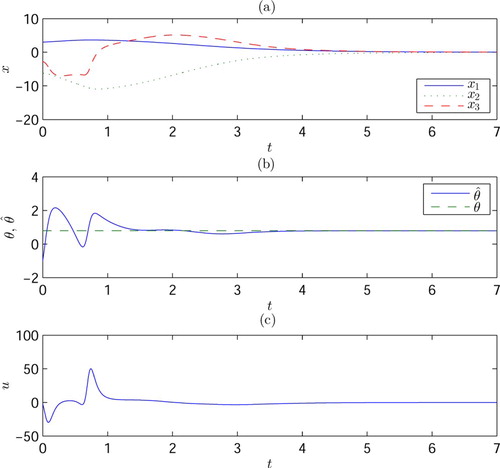
Figure 2. Simulation results for Case B.

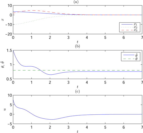
It can be observed from the simulation results that

1. the forms of the responses of this nonlinear system are quite different from that of a linear system;

2. the responses of the system depend more heavily on the initial values.

Due to paper length, treatment of this example system by second-order method of backstepping is omitted.

7. Conclusion

The paper proposes a HOFA approach for adaptive control of nonlinear systems with unknown parameters, and has demonstrated the following:

• Many nonlinear systems with an unknown parameter vector can be represented by either a single HOFA model with unknown parameters or second- and/or high-order SFSs with unknown parameters. As a result, the well-known first-order SFSs with unknown parameters, as well as the newly proposed second- and high-order uncertain SFSs with unknown parameters, are also system models closely related to uncertain HOFA models for nonlinear systems since each of their subsystem obey a full-actuation structure.

• Due to the full-actuation feature of the HOFA models, effective designs of adaptive controllers for nonlinear systems with unknown parameters are proposed. It is demonstrated by a benchmark problem that the HOFA approach turns out to be extremely simple and is not subject to the problem of over-parameterisation.

• For the cases of second- and high-order SFSs with unknown parameters, the designs turn out to be the generalised second- and high-order methods of backstepping for second- and high-order SFSs, correspondingly.

• The proposed approach possesses several merits, particularly, the state vectors converge globally to the origin, and in the case of a single HOFA model, the closed-loop system becomes a constant linear one with an arbitrarily assignable eigenstructure when the unknown parameters do not present.

The proposed second- and high-order methods of backstepping for second- and high-order SFSs can be further generalised to the case that both $x_i$ and ${\vartheta }_i,$ $i=1,2,\dots ,n$ are vectors.

Acknowledgments

The author is grateful to his Ph.D. students, Tianyi Zhao, Guangtai Tian, Qin Zhao, Xiubo Wang, etc., for helping him with reference selection and proofreading.

Disclosure statement

No potential conflict of interest was reported by the author.

Additional information

Funding

This work has been partially supported by the Major Program of National Natural Science Foundation of China [grant numbers 61690210, 61690212], the National Natural Science Foundation of China [grant number 61333003] and the Self-Planned Task of State Key Laboratory of Robotics and System (HIT) [grant number SKLRS201716A].

Notes on contributors

Guangren Duan

Guangren Duan received his Ph.D. degree in Control Systems Sciences from Harbin Institute of Technology, Harbin, P. R. China, in 1989. After a two-year post-doctoral experince at the same university, he became professor of control systems theory at that university in 1991. He is the founder and currently the Director of the Center for Control Theory and Guidance Technology at Harbin Institute of Technology. He visited the University of Hull, the University of Sheffield, and also the Queen's University of Belfast, UK, from December 1996 to October 2002, and has served as Member of the Science and Technology committee of the Chinese Ministry of Education, Vice President of the Control Theory and Applications Committee, Chinese Association of Automation (CAA), and Associate Editors of a few international journals. He is currently an Academician of the Chinese Academy of sciences, and Fellow of CAA, IEEE and IET. His main research interests include parametric control systems design, nonlinear systems, descriptor systems, spacecraft control and magnetic bearing control. He is the author and co-author of 5 books and over 270 SCI indexed publications.

References

- Astolfi, A., Karagiannis, D., & Ortega, R. (2008). Nonlinear and adaptive control with applications. Springer-Verlag.
- Aström, K. J. (1980). Design principles for self-tuning regulators. In Methods and applications in adaptive control. Springer.
- Aström, K. J., & Wittenmark, B. (1995). Adaptive control (2nd ed.). Addison-Wesley.
- Brown, M., & Harris, C. (1994). Neuro fuzzy adaptive modelling and control. Prentice Hall.
- Chan, S. W., & Goodwin, G. C. (1982). On the role of the interactor matrix in MIMO adaptive control. IEEE Transactions on Automatic Control, 27(6), 713–714. https://doi.org/10.1109/TAC.1982.1102960
- Cui, G. Y. (2010). Ordinary differential equations: Theory, modeling and development. Tsinghua University Press.
- Ding, Z. T. (2013). Nonlinear and adaptive control systems. IET.
- Duan, G. R. (1992). Simple algorithm for robust pole assignment in linear output feedback. IEE Proceedings D: Control Theory and Applications, 139(5), 465–470. https://doi.org/10.1049/ip-d.1992.0058
- Duan, G. R. (1993). Robust eigenstructure assignment via dynamical compensators. Automatica, 29(2), 469–474. https://doi.org/10.1016/0005-1098(93)90140-O
- Duan, G. R. (2015). Generalized Sylvester equations: Unified parametric solutions. CRC Press.
- Duan, G. R. (2020a). High-order system approaches – I. Full-actuation and parametric design. Acta Automatica Sinica, 46(7), 1333–1345. (in Chinese). https://doi.org/10.16383/j.aas.c200234
- Duan, G. R. (2020b). High-order system approaches – II. Controllability and fully-actuation. Acta Automatica Sinica, 46(8), 1571–1581. (in Chinese). https://doi.org/10.16383/j.aas.c200369
- Duan, G. R. (2020c). High-order system approaches – III. Super-observability and observer design. Acta Automatica Sinica, 46(9). (in Chinese). https://doi.org/10.16383/j.aas.c200370
- Duan, G. R. (2020d). High-order fully-actuated system approaches: I. Models and basic procedure. International Journal of System Sciences. https://doi.org/10.1080/00207721.2020.1829167
- Duan, G. R. (2020e). High-order fully-actuated system approaches: II. Generalized strict-feedback systems. International Journal of System Sciences. https://doi.org/10.1080/00207721.2020.1829168
- Duan, G. R. (2020f). High-order fully-actuated system approaches: III. Robust control and high-order backstepping. International Journal of System Sciences.
- Duan, G. R., Irwin, G. W., & Liu, G. P. (2002). Disturbance attenuation in linear systems via dynamical compensators: A parametric eigenstructure assignment approach. IEE Proceedings-Control Theory and Applications, 147(2), 129–136. https://doi.org/10.1049/ip-cta:20000135
- Duan, G. R., Liu, G. P., & Thompson, S. (2000). Disturbance attenuation in luenberger function observer designs – A parametric approach. IFAC Proceedings Volumes, 33(14), 41–46. https://doi.org/10.1016/S1474-6670(17)36202-X
- Duan, G. R., & Zhao, T. Y. (2020). Observer-based multi-objective parametric design for spacecraft with super flexible netted antennas. Science China Information Sciences, 63(172002), 1–21. https://doi.org/10.1007/s11432-020-2916-8
- Fantoni, I., & Lozano, R. (2002). Nonlinear control for underactuated mechanical systems. Springer-Verlag.
- Farrell, J. A., & Polycarpou, M. M. (2006). Adaptive approximation based control: Unifying neural, fuzzy, and traditional adaptive approximation approaches. John Wiley and Sons.
- Feuer, A., & Morse, A. S. (1978). Adaptive control of single-input single-output linear systems. IEEE Transactions on Automatic Control, 23(4), 557–569. https://doi.org/10.1109/TAC.1978.1101822
- Fradkov, A. L., Miroshnik, I. V., & Nikiforov, V. O. (1999). Nonlinear and adaptive control of complex systems. Springer.
- Ge, S. S., Hang, C. C., Lee, T. H., & Zhang, T. (2001). Stable adaptive neural network control. Kluwer Academic.
- Goodwin, G. C., & Long, R. S. (1980). Generalization of results on multivariable adaptive control. IEEE Transactions on Automatic Control, 25(6), 1241–1245. https://doi.org/10.1109/TAC.1980.1102523
- Goodwin, G. C., Ramadge, P. J., & Caines, P. E. (1980). Discrete-time multivariable adaptive control. IEEE Transactions on Automatic Control, 25(6), 449–456. https://doi.org/10.1109/TAC.1980.1102363
- Goodwin, G. C., & Sin, K. S. (1984). Adaptive filtering prediction and control. Prentice-Hall.
- Isidori, A. (1995). Nonlinear control systems (3rd ed.). Springer-Verlag.
- Jiang, Z. P., & Praly, L. (1991). Iterative designs of adaptive controllers for systems with nonlinear integrators. In Proceedings of the 30th IEEE Conference on Decision and Control (pp. 2482–2487).
- Kanellakopoulos, I., Kokotović , P. V., & Morse, A. S. (1991). Systematic design of adaptive controllers for feedback linearizable systems. IEEE Transactions on Automatic Control, 36(11), 1241–1253. https://doi.org/10.1109/9.100933
- Kokotović, P. V. (1991). Foundations of adaptive control. Springer-Verlag.
- Kokotović, P. V., & Arcak, M. (2001). Constructive nonlinear control: A historical perspective. Automatica, 37(5), 637–662. https://doi.org/10.1016/S0005-1098(01)00002-4
- Kokotović, P. V., Kanellakopoulos, I., & Morse, A. S. (1991). Adaptive feedback linearization of nonlinear systems. In Foundations of adaptive control (pp. 309–346). Springer.
- Kokotović, P. V., & Kanellakopoulos, I. (1990). Adaptive nonlinear control: A critical appraisal. In Proceedings of the Sixth Yale Workshop on Adaptive and Learning Systems (pp. 1–6).
- Krstić, M., Kanellakopoulos, I., & Kokotović, P. V. (1992). Adaptive nonlinear control without overparametrization. Systems and Control Letters, 19(3), 177–185. https://doi.org/10.1016/0167-6911(92)90111-5
- Krstić, M., Kanellakopoulos, I., & Kokotović, P. V. (1995). Nonlinear and adaptive control design. John Wiley and Sons.
- Landau, Y. D. (1979). Adaptive control: The model reference approaches. Marcel Dekker.
- Lewis, F. L., Campos, J., & Selmic, R. (2002). Frontiers in applied mathematics, neurofuzzy control of industrial systems with actuator nonlinearities. SIAM.
- Marino, R., & Tomei, P. (1995). Nonlinear control design: Geometric, adaptive and robust. Prentice-Hall.
- Monopoli, R. V., & Hsing, C. C. (1975). Parameter adaptive control of multivariable systems. International Journal of Control, 22(3), 313–327. https://doi.org/10.1080/00207177508922087
- Morris, K. (1978). Mathematical thought from ancient to modern times. Oxford University Press.
- Mosca, E. (1995). Optimal, predictive, and adaptive control. Prentice-Hall.
- Nassiri-Toussi, K., & Ren, W. (1997). Indirect adaptive pole-placement control of MIMO stochastic systems: self-tuning results. IEEE Transactions on Automatic Control, 42(1), 38–52. https://doi.org/10.1109/9.553686
- Sastry, S., & Isidori, A. (1989). Adaptive control of linearizable systems. IEEE Transactions on Automatic Control, 34(11), 1123–1131. https://doi.org/10.1109/9.40741
- Seto, D., Annaswamy, A., & Baillieul, J. (1994). Adaptive control of nonlinear systems with a triangular structure. IEEE Transactions on Automatic Control, 39(7), 1411–1428. https://doi.org/10.1109/9.299624
- Seto, D., & Baillieul, J. (1994). Control problems in super-articulated mechanical systems. IEEE Transactions on Automatic Control, 39(12), 2442–2453. https://doi.org/10.1109/9.362851
- Spooner, J. T., Maggiore, M., Ordsqez, R., & Passino, K. M. (2002). Stable adaptive control and estimation for nonlinear systems: Neural and fuzzy approximator techniques. John Wiley and Sons.
- Tao, G. (2003). Adaptive control design and analysis. John Wiley and Sons.
- Tao, G. (2014). Multivariable adaptive control: A survey. Automatica, 50(11), 2737–2764. https://doi.org/10.1016/j.automatica.2014.10.015
- Zhang, H. G., & Liu, D. R. (2006). Fuzzy modelling and fuzzy control. Birkhauser.
- Zhou, J., & Wen, C. (2008). Adaptive backstepping control of uncertain systems, nonsmooth nonlinerities, interactions or time-variations. Springer-Verlag.