
 ?Mathematical formulae have been encoded as MathML and are displayed in this HTML version using MathJax in order to improve their display. Uncheck the box to turn MathJax off. This feature requires Javascript. Click on a formula to zoom.
Abstract
Two types of high-order fully actuated (HOFA) system models subject to external disturbances are firstly introduced. For the type of HOFA systems with deterministic disturbances, the problem of disturbance attenuation via state feedback is treated. While for the type of HOFA systems with dynamical disturbances, the problem of asymptotic disturbance decoupling via output feedback is considered. Utilising the full-actuation feature of the HOFA systems, disturbance attenuation and decoupling controllers for the corresponding systems are conveniently designed such that constant linear closed-loop systems with designed disturbance rejection properties are resulted in. Parametric designs for both controllers are provided, and disturbance attenuation is achieved by establishing a parametric form of the closed-loop transfer function from the disturbance to the output, while the parametric form of the disturbance decoupling controller is derived based on a complete parametric solution to a type of generalised Sylvester equations (GSEs). As a consequence of the parameter approaches, additional performance requirements on the closed-loop systems can be also easily handled. An illustrative example demonstrates the effect of the proposed approach.
1. Introduction
Disturbance attenuation and decoupling are important issues in the field of control theory, and have attracted much attention of control scientists and engineers. As is claimed in Gao (Citation2014) that ‘the problem of automatic control is, in essence, that of disturbance rejection’.
1.1. A brief overview on disturbance rejection
In many applications, we encounter systems with completely unknown disturbances. In such applications, attenuation of the effect of the disturbances on the output of the system is desired.
1.1.1. Disturbance attenuation
There are many excellent results on disturbance attenuation in the history. In J. Huang (Citation1995), a robust control law is proposed for a type of uncertain nonlinear systems, which can realise local asymptotic tracking and disturbance rejection regardless of certain plant uncertainties. The similar problem is also considered for fully actuated passive mechanical systems in Jayawardhana and Weiss (Citation2008).
and
techniques are two of the mainstream methods to solve the problem of disturbance attenuation. In the celebrated works, Zhou et al. (Citation1994) and Doyle et al. (Citation1994), the mixed
and
performance control for linear systems is transformed into a problem of solving a type of Ricatti equations. Another type of solution is the linear matrix inequality (LMI) approach, the
and
control problems are treated by many scholars through solving a group of LMIs, and a great deal of systematic results are obtained (see Duan & Yu, Citation2013 and the references therein). Regarding nonlinear systems,
control problem is considered for the case of measurement output feedback in Isidori and Astolfi (Citation1992) and Ball et al. (Citation1993). Wang et al. (Citation2009) and Wang et al. (Citation2012) develop a robust
controller and a quantised
controller, respectively, for a class of nonlinear discrete time-delay stochastic systems with missing measurements.
Another type of approaches for disturbance attenuation in linear systems is the so-called parametric approaches. These include the case of model reference tracking (L. Huang et al., Citation2006), second-order systems (Duan & Huang, Citation2006), dynamic compensator (Duan et al., Citation2002) and Luenberger function observer (Duan et al., Citation2000a).
Adaptive control is also applied successfully to solve the disturbance rejection problem for certain type of uncertain nonlinear systems, e.g. Marino and Tomei (Citation2005), and the idea is also extended to some generalised high-order uncertain nonlinear systems in Sun et al. (Citation2017).
Active disturbance rejection control (ADRC) is another effective way to the problem of disturbance attenuation, and many valuable results are obtained in the past decades (see the review paper Y. Huang & Xue, Citation2014 and the references therein). Recently, the ADRC technique is applied to a type of uncertain time-delay nonlinear systems in Ran et al. (Citation2020), and a predictive ADRC law is presented, which makes the closed-loop system achieve local convergence under certain conditions.
1.1.2. Disturbance decoupling
Regarding disturbance decoupling, there are also many reported results. For linear systems, a series of systematic methods are presented in the book (Saberi et al., Citation2000). For nonlinear systems, the problem of disturbance decoupling maybe originally proposed and investigated in Huijberts et al. (Citation1992) by making an analogy with the dynamic input-output decoupling problem, and a local solution to this problem is obtained in the case that the system under consideration is invertible. The case of output feedback is further considered for continuous- and discrete-time nonlinear systems in Andiarti and Moog (Citation1996) and Kaldmae et al. (Citation2013), respectively. In Kaldmae et al. (Citation2018), the systems under consideration are generalised to a type of nonlinear hybrid ones, and sufficient conditions are given, under which there exists a dynamic measurement feedback such that the controlled output is completely decoupled from the disturbances. Some other types of nonlinear systems, such as switched systems (Zheng et al., Citation2005) and time-delay systems (Moog et al., Citation2000; Velasco et al., Citation1997), are also investigated in depth.
Parametric approaches have also been proposed for disturbance decoupling. For instance, Duan et al.(Citation1997) proposed a parametric design method for the problem of disturbance decoupling and simultaneously applied it to fault diagnosis. Moreover, disturbance decoupling problem of singular linear systems for the case of output feedback is also dealt with (Duan et al., Citation2000b).
Since disturbance decoupling may not be achieved in many practical situations, the concept of almost disturbance decoupling is proposed and investigated by certain scholars. The case of single-input single-output nonlinear systems is considered first in Marino et al. (Citation1989), and then the result is extended to multiple-input multiple-output nonlinear systems in Liu et al. (Citation2004). The output feedback case is investigated in Marino and Tomei (Citation2000), and some type of high-order nonlinear systems are treated in Qian and Lin (Citation2000).
It is well-known that, for many nonlinear systems, global stabilisation can be seldom achieved with the commonly used state-space models of the dynamical systems, while disturbance attenuation and decoupling are generally dependent on the stabilisation of the system. Therefore, many disturbance attenuation and decoupling results for nonlinear control systems, such as J. Huang (Citation1995), Isidori and Astolfi (Citation1992) and Ran et al. (Citation2020), can only be obtained in a local sense.
1.2. The HOFA system approaches
A common fact lies in the above mentioned results on disturbance attenuation and decoupling is that they all fall into the general framework of first-order state-space approaches. For over half a century time of dominance, state-space models have been regarded as universal. Most control scientists and practitioners have been accustomed to convert any system encountered into a state-space representation. Like most other achievements in control systems theory, almost all results on disturbance rejection in the literature are based on the first-order state-space models. However, as argued and demonstrated in Duan (Citation2021a, Citation2021b, Citation2021c, Citation2020a, Citation2020b, Citation2020c,Citation2020d, Citation2021d), the first-order state-space model, although is very suitable for state solutions, is not the best choice for dealing with the control problems.
In Duan (Citation2021a, Citation2020a), the type of HOFA models for dynamical systems is introduced, together with the HOFA approaches for dynamical system control. Like the state-space models for dynamical control systems, a HOFA model serves as also a general representation of a control system. Generally speaking, the former is more suitable for deriving the state solution and observation, while the latter has been shown to be extremely convenient and effective for dealing with the control of dynamical systems (Duan, Citation2020b, Citation2020c, Citation2020d, Citation2021d), the full-actuation feature of a HOFA model provides a great deal of convenience and also significant improvement on the designed results. As long as the nonlinearities in the system are known, a controller can be sought which cancels the nonlinearities and hence makes the closed-loop system a constant linear one with an arbitrarily assignable eigenstructure.
In this paper, an HOFA approach for disturbance attenuation and decoupling is proposed. It is well known that the problem of disturbance rejection heavily depends on the stabilisation of the systems, while for many nonlinear systems global stabilisation can be seldom achieved with the commonly used state-space model representation of the dynamical systems. Utilising the full-actuation feature of the HOFA models, the problem of disturbance attenuation and decoupling in a nonlinear system can be converted into a problem of disturbance attenuation and decoupling in a linear system. Hence the ideas in the parametric approaches for disturbance attenuation and decoupling in linear systems (see, e.g. Duan & Huang, Citation2006; Duan et al., Citation2002, Citation1997; L. Huang et al., Citation2006), can be effectively applied. Along this general line, the problem of disturbance attenuation and asymptotic disturbance decoupling in nonlinear HOFA systems is completely solved, and parametric solutions to the problems of disturbance attenuation and asymptotical decoupling are proposed.
The contribution of the paper is composed of two aspects. Firstly, based on a parametric state feedback controller for HOFA systems, a parametric form of the norm of the transfer function, from the disturbance to the output of the closed-loop system, is established, and minimisation of the
norm of the transfer function is then readily realised. Secondly, using complete parametric solutions to a type of nonhomogeneous generalised Sylvester equations (GSEs), a parametric approach is also established for asymptotic disturbance decoupling in an HOFA system with a dynamical disturbance.
In the sequential sections, denotes the identity matrix,
and
denote the determinant and adjoint matrix of a matrix A, respectively. For
and
as in Duan (Citation2020c), the following symbols are used in the paper:
The paper is organised into six sections. In the next section the two types of HOFA models with disturbances are introduced, and in Sections 3 and 4 the problems of disturbance attenuation and decoupling are investigated, respectively. Section 5 presents an illustrative example, followed by a brief concluding remark.
2. HOFA models
In this section, two types of HOFA models for dynamical systems with disturbances are proposed on the basis of a type of uncertain HOFA models introduced in the Part II of the series (Duan, Citation2020b).
2.1. Uncertain HOFA models
Consider the following HOFA model introduced in Duan (Citation2020b):
(1)
(1)
where
is an integer, x,
are the state vector and the control input vector, respectively,
may represent a parameter vector, an external variable vector, a time-delayed state vector, an unmodeled dynamic state vector, etc.;
is a known sufficiently smooth vector function, while
is an unknown term,
is a sufficiently smooth matrix function satisfying the following full-actuation condition:
Assumption A1 .
From appearance, the above Assumption A1 seems to be strict. While as a matter of fact, the above HOFA system (Equation1(1)
(1) ) represents a quite general model for ‘completely controllable’ systems, and can either be obtained through physical modelling, or through conversion from other types of models (Duan, Citation2021a,Citation2021b, Citation2020a, Citation2020b, Citation2020c, Citation2020d, Citation2021d).
As a demonstration, let us restate that the following uncertain strict-feedback system can be converted into the form of (Equation1(1)
(1) ):
(2)
(2)
where
,
are the state vectors,
is the control input,
and
,
are sufficiently smooth vector functions, and
,
are a set of nonsingular matrices. According to the Theorem 3.1 or 3.6 in Duan (Citation2020b), we have the following simplified result.
Proposition 2.1
The above strict-feedback system (Equation2(2)
(2) ), with
,
being nonsingular, can be transformed into the form of
(3)
(3)
with
, and
(4)
(4)
(5)
(5)
(6)
(6)
where
and in (Equation5
(5)
(5) ) and (Equation6
(6)
(6) ) the
and their derivatives are all given or determined by certain transformation (see the Theorem 3.1 in Duan, Citation2020b).
Similarly, it can be shown via the Theorems 3.2, 3.3 and 3.6 in Duan (Citation2020b) that the second- and high-order strict-feedback systems proposed in Duan (Citation2020b), with uncertainties properly added, can be also converted into the form of the HOFA system (Equation1(1)
(1) ).
2.2. HOFA models with deterministic disturbances
Now let us consider the case where is a deterministic external disturbance. In such a case we may assume
(7)
(7)
where
is an external disturbance, depending only on time t,
is a known constant distribution matrix. Therefore, the uncertain system (Equation1
(1)
(1) ) becomes the following one with a deterministic disturbance:
(8)
(8)
Again, the above HOFA system (Equation8
(8)
(8) ) can be either obtained through physical modelling (see the two examples in Duan (Citation2020b), and also the example in the Section 5 of this present paper), or through conversion from other types of models (Duan, Citation2021a, Citation2021b, Citation2020a, Citation2020b).
Parallelly, taking
in (Equation2
(2)
(2) ), where
and
are the external disturbances and the constant distribution matrices, respectively, gives the following strict-feedback system with disturbances:
(9)
(9)
Following the above Proposition 2.1, we can convert the above strict-feedback system into a HOFA system in the form of
(10)
(10)
with
and
being given by (Equation4
(4)
(4) ) and (Equation5
(5)
(5) ), respectively, and
being determined by (Equation6
(6)
(6) ) as
(11)
(11)
Similarly, it can be shown via the Theorems 3.2, 3.3 and 3.6 in Duan (Citation2021a, Citation2021b, Citation2020a, Citation2020b) that the second- and high-order strict-feedback systems proposed in Duan (Citation2021a, Citation2021b, Citation2020a, Citation2020b), with disturbances added, can be also converted into the form of (Equation8
(8)
(8) ).
Remark 2.1
It is clearly seen from (Equation11(11)
(11) ) that some constant disturbances, slope disturbances, etc., may automatically disappear when the HOFA system method is used for design. Therefore, the HOFA system approach itself has certain ‘natural’ anti-disturbance characteristics. In certain situations, the control of a system subject to disturbances can be turned in a control problem free of disturbances (see the examples in Duan (Citation2021a, Citation2021b, Citation2020a, Citation2020b)).
2.3. HOFA models with dynamical disturbances
Inspired by the form of (Equation11(11)
(11) ), we introduce the following HOFA model with a disturbance:
(12)
(12)
where the disturbance
is generated by some exogenous system
(13)
(13)
which can be also expressed into the following state-space form:
(14)
(14)
Here we mention that
is generally assumed to be not Hurwitz, since otherwise the disturbance
will eventually die out automatically.
Example 2.2
Let us consider the disturbance
where c and ω are two positive scalars. Note that
this particular disturbance can be modelled by
which can be express as
(15)
(15)
with
(16)
(16)
The model (Equation15
(15)
(15) ) and (Equation16
(16)
(16) ) can be also equivalently expressed in the following state-space form:
with
Remark 2.2
For the HOFA model (Equation8(8)
(8) ) with a deterministic disturbance and the HOFA model (Equation12
(12)
(12) ) and (Equation13
(13)
(13) ) with a dynamical disturbance, many practical examples exist at least for the second-order system case. For the HOFA model (Equation8
(8)
(8) ) with a deterministic disturbance, we aim to consider the problem of disturbance attenuation since no further information about the disturbance is known. For the HOFA model (Equation12
(12)
(12) ) and (Equation13
(13)
(13) ) with a dynamical disturbance, we can realise asymptotical disturbance decoupling based on the dynamical model of the disturbance.
3. Disturbance attenuation
Adding an output equation to the system (Equation8(8)
(8) ), gives the following HOFA model:
(17)
(17)
where
is the system output,
is a constant measurement matrix.
In this section, we will consider the disturbance attenuation problem in the above system (Equation17(17)
(17) ).
3.1. Problem statement
For the above high-order system (Equation17(17)
(17) ) with a disturbance
, if we design the following control law
(18)
(18)
then it can be easily verified that the closed-loop system is
(19)
(19)
which can be also rewritten, more compactly, as
(20)
(20)
Further denote
(21)
(21)
the above Equation (Equation20
(20)
(20) ) can be also equivalently transformed into the following state-space form
(22)
(22)
The above deduction states a very important fact: once a nonlinear system is represented into a HOFA model, a controller for the system can be easily designed using the full-actuation feature of the HOFA model such that the closed-loop system becomes a constant linear one subject to the same disturbance. Hence the disturbance attenuation problem for a nonlinear HOFA system is turned into one for a linear system.
With the above preparation, the disturbance attenuation problem to be considered in this section is to design the matrix such that the above linear system (Equation22
(22)
(22) ) has an anti-disturbance property. This can be stated as follows.
Problem 3.1
For a given HOFA system (Equation17(17)
(17) ), determine the coefficient matrix
in the control law (Equation18
(18)
(18) ) such that
(23)
(23)
is minimised, where
is the transfer function from d to y defined by
(24)
(24)
Since problem (Equation23(23)
(23) )–(Equation24
(24)
(24) ) is a standard
or
problem for linear systems, many existing methods can be readily applied, e.g. the Ricatti equation approach (Doyle et al., Citation1994; Zhou et al., Citation1994), and the LMI approach (see, e.g.Duan & Yu, Citation2013). In this section, we will present a complete parametric approach for the
problem. The idea is to first establish a complete parametric solution of
, and then to give a parametric expression of
based on the parameters Z and F existing in the general parametric solution of
.
3.2. Preliminaries
To derive our main results, three preliminary results are needed. The first one is about the solution to the following GSE:
(25)
(25)
Lemma 3.1
For an arbitrarily selected matrix all the matrices
and
satisfying the above equation (Equation25
(25)
(25) ) are given by
(26)
(26)
where
is an arbitrary parameter matrix.
The above result can be easily proven using the Theorem 4.3 in Duan (Citation2015, p. 120), about the parametric solution to a general GSE.
The second preliminary result gives an analytical expression of the norm of a transfer function in terms of solutions to Lyapunov matrix equations (see, e.g. the Lemma 5.1 in Duan and Yu (Citation2013, p. 140)).
Lemma 3.2
Let ,
,
and A be Hurwitz. Then
where
and
are the unique positive definite solutions to the following Lyapunov equations
and
respectively.
Introduce the following notations related to a square matrix :
Then we have the following result which is simplified from the Theorem 9.2 in Duan (Citation2015, p. 356).
Lemma 3.3
If is Hurwitz, then, for an arbitrary positive definite matrix
the following Lyapunov equation
has a unique solution given by
(27)
(27)
with
(28)
(28)
3.3. Parametric solution
Now let us turn to consider the solution to the problem.
3.3.1. Explicit solution of 
Regarding a parametric solution of the coefficient matrix in the controller (Equation18
(18)
(18) ), we have the following result.
Theorem 3.4
For an arbitrarily selected matrix all the matrices
and
satisfying
and
(29)
(29)
are given by
(30)
(30)
and (Equation26
(26)
(26) ), with
being a parameter matrix satisfying
(31)
(31)
Proof.
Write Equation (Equation29(29)
(29) ) as
(32)
(32)
Further, introducing the variable
(33)
(33)
and in view of
(34)
(34)
we can convert equivalently the above equation (Equation32
(32)
(32) ) into the form of (Equation25
(25)
(25) ). Therefore, it follows from Lemma 3.1 that all the matrices V and W are given by (Equation26
(26)
(26) ), and equation (Equation30
(30)
(30) ) can then be further solved from (Equation33
(33)
(33) ).
Remark 3.1
The above theorem clearly establishes a general parametric solution of the controller (Equation18(18)
(18) ), which arbitrarily assigns the desired eigenstructure of the closed-loop system (Equation22
(22)
(22) ). It is actually a result on eigenstructure assignment in the linear system
which is termed as the ‘basic problem’ in Duan (Citation2021a) (see, also the Corollary 1 in Duan (Citation2020b), or refer to Duan (Citation2020b, Citation2020c)),
3.3.2. Parametric expression of
Based on Lemmas 3.2 and 3.3, and Theorem 3.4, the following result can be obtained, which gives a parametric expression of the norm of the transfer function (Equation24
(24)
(24) ).
Theorem 3.5
Let be a given Hurwitz matrix, and
and
are determined by
(35)
(35)
and
(36)
(36)
respectively. If the control law for the HOFA system (Equation17
(17)
(17) ) is taken as (Equation18
(18)
(18) ), with
being given by (Equation30
(30)
(30) ), then we have
(37)
(37)
where V is given by (Equation26
(26)
(26) ), and
(38)
(38)
with
(39)
(39)
Proof.
When the control law (Equation18(18)
(18) ), with
chosen as in (Equation30
(30)
(30) ), applied to system (Equation17
(17)
(17) ), the closed-loop system can be obtained and rewritten in the state-space form (Equation22
(22)
(22) ). It follows from Theorem 3.4 that (Equation29
(29)
(29) ) holds. Thus, substituting (Equation29
(29)
(29) ) into (Equation24
(24)
(24) ), yields
(40)
(40)
Considering that the matrix F is Hurwitz, there exists unique positive definite solutions
and
satisfying the following Lyapunov equations
(41)
(41)
and
(42)
(42)
respectively. According to Lemma 3.3, the matrices
and
given by (Equation38
(38)
(38) ) – (Equation39
(39)
(39) ) are, respectively, the solutions to the Lyapunov equations (Equation41
(41)
(41) ) and (Equation42
(42)
(42) ). Therefore, it follows from Lemma 3.2 that
is given by (Equation37
(37)
(37) )–(Equation39
(39)
(39) ). The proof is then completed.
With the help of the above two theorems, solution to the disturbance problem in system (Equation17(17)
(17) ) via the controller (Equation18
(18)
(18) ) can then be solved by optimising the design parameters F and Z to minimise
. Clearly, an advantage of the parametric approach is that it is easy to have additional indices to be comprehensively optimised together with this
index.
In applications, it suffices to choose F to be a diagonal matrix with negative diagonal elements. In the case that complex eigenvalues are expected, we may have such a block
(43)
(43)
with a and b being two positive scalars, included as a diagonal block in F.
Clearly, there are quite some degrees of freedom in the selection of F, while on the other hand we also have the parameter matrix Z, which provides degrees of freedom. All these degrees of freedom can be further utilised to achieve additional performance of the system (see, e.g.Duan, Citation1992a, Citation1993b; Duan et al., Citation2002, Citation2000a; Duan & Zhao, Citation2020).
4. Asymptotic disturbance decoupling
Adding two output equations to the system (Equation12(12)
(12) ), and replacing the state
in the system by the measured output
, gives the following HOFA system:
(44)
(44)
where
is the measured output,
is the regulated output,
and
are the coefficient matrices of appropriate dimensions, and the disturbance
is generated by the exogenous system (Equation13
(13)
(13) ), or equivalently, the state-space system (Equation14
(14)
(14) ).
In this section, asymptotic disturbance decoupling in the above system (Equation44(44)
(44) ) is considered via dynamical output feedback. The aim is to find a control law, employing the feedback of the measured output
for the given HOFA system (Equation44
(44)
(44) ) with the disturbance d generated by the exogenous system (Equation13
(13)
(13) ), such that the following asymptotic output regulation requirement
(45)
(45)
is met for arbitrary initial values
and
.
To solve this problem, we also need some preliminary results.
4.1. Preliminary results
Let us first state a result about disturbance attenuation in linear systems.
4.1.1. Disturbance decoupling in linear systems
Consider the following linear system
(46)
(46)
where
and
are the state and the control input, respectively;
and
are the measured output and the regulated output, respectively;
is the disturbance generated by the following exogenous system
(47)
(47)
where the matrix S is usually not Hurwitz since otherwise the disturbance w dies out itself. Furthermore, the system coefficient matrices are assumed to satisfy the following conditions.
Condition C1 The matrix pair is stabilisable.
Condition C2 The matrix pair is detectable, where
The following lemma is a simplified version of the Theorem 2.4.1 in Saberi et al. (Citation2000, p. 25) (see, also the Theorem 2.6 in Duan (Citation2015, p.51)), which gives a basic output regulation result for the linear system (Equation46(46)
(46) ).
Lemma 4.1
Suppose that the system (Equation46(46)
(46) ) satisfies Conditions C1–C2. Let the control law for the system be designed as
(48)
(48)
where
and
are arbitrary matrices making
(49)
(49)
both Hurwitz; Γ and Π are the solutions to the following matrix equations:
(50)
(50)
(51)
(51)
Then,
| (1) | the following closed-loop system is internally asymptotically stable
| ||||
| (2) | the following asymptotic output regulation requirement
| ||||
4.1.2. Solution to a GSE
In this subsection, let us give a general parametric solution to the following nonhomogeneous GSE:
(54)
(54)
Lemma 4.2
Let
. Then all the matrices
and
satisfying Equation(Equation54
(54)
(54) ) are given by
(55)
(55)
where
is an arbitrary parameter matrix.
Proof.
Obviously, the homogeneous equation of the above GSE (Equation54(54)
(54) ) is Equation (Equation25
(25)
(25) ). Let
be a general solution to the homogeneous GSE (Equation25
(25)
(25) ), and
be a particular solution to the above GSE (Equation54
(54)
(54) ), then it is easily known that the general solution
to the above nonhomogeneous equation (Equation54
(54)
(54) ) is given by
(56)
(56)
It follows from Lemma 3.1 that a general solution to the homogeneous GSE (Equation25
(25)
(25) ) is given by (Equation26
(26)
(26) ). Further, it can be easily verified that a particular solution to the above nonhomogeneous GSE (Equation54
(54)
(54) ) is given by
(57)
(57)
Therefore, the general solution (Equation55
(55)
(55) ) immediately follows from (Equation26
(26)
(26) ), (Equation56
(56)
(56) ) and (Equation57
(57)
(57) ).
4.2. Parametric solution
It is obvious that is controllable. Further denote
(58)
(58)
then we also need the following assumption:
Assumption A2 The matrix pair defined by (Equation58
(58)
(58) ) is detectable.
Let us introduce the following control law for the HOFA system (Equation44(44)
(44) ):
(59)
(59)
where
(60)
(60)
and
(61)
(61)
with
and
being some parameter matrices. Applying Lemmas 3.1, 4.1 and 4.2, we can obtain the following result.
Theorem 4.3
Let the HOFA system (Equation44(44)
(44) ), with the disturbance
generated by (Equation13
(13)
(13) ), satisfies Assumption A1. If the control law is taken as (Equation59
(59)
(59) )–(Equation61
(61)
(61) ), with the parameter matrices
,
and
satisfying the following conditions:
| (1) |
| ||||
| (2) | the parameter | ||||
| (3) | the parameter | ||||
Proof.
If we take the following control law
(66)
(66)
then the corresponding closed-loop system is given by
(67)
(67)
The above Equation (Equation67
(67)
(67) ) can be also equivalently rewritten in the following state-space form:
(68)
(68)
It is noted that the above (Equation68
(68)
(68) ) is now a constant linear system. Applying Lemma 4.1 to the above system (Equation68
(68)
(68) ), we can design the following controller v to meet the asymptotic output regulation requirement (Equation45
(45)
(45) ):
(69)
(69)
where the matrices
and
satisfy the first condition in the theorem,
makes the matrix
stable, while Π and Γ are two matrices satisfying the following two equations
(70)
(70)
and
(71)
(71)
Combining the above controller (Equation69
(69)
(69) ) with (Equation66
(66)
(66) ), gives the controller (Equation59
(59)
(59) ). Further, it is easy to see that the following three facts hold:
according to Theorem 3.4 that the matrix
applying Lemma 4.2, with F and R substituted by
with the matrices Π and Γ given by (Equation61
With the above three facts, we immediately have the conclusion of the theorem.
Remark 4.1
The above theorem has provided a parametric approach for the problem of disturbance decoupling in the HOFA system (Equation17(17)
(17) ). The design degrees of freedom are explicitly given by the parameters
and
which can be further properly selected to meet additional performance requirements of the closed-loop system. It should be also noted that explicit parametric solutions of
and
satisfying the first condition in the above Theorem 4.5 can be also readily established using state feedback eigenstructure assignment results for linear systems (see, Duan, Citation1992b, Citation1993a, Citation1998, Citation2004, Citation2005). We point out that there exist usually also certain degrees of freedom in the solution of
and
satisfying the first condition in the theorem, and the case of dynamic state feedback will be further addressed in the next subsection.
4.3. Case of dynamical state feedback
In the case of we have
, and the controller (Equation59
(59)
(59) ) turns into a dynamical state feedback controller. In this subsection, we aim to further give a parametric solution to the design of
and
satisfying the first condition in Theorem 4.3 in the case of dynamical state feedback.
Firstly, let us give a necessary and sufficient condition for the observability (detectability) of the matrix pair defined by
(72)
(72)
Theorem 4.4
The matrix pair defined by (Equation72
(72)
(72) ) is observable (detectable) if and only if
is observable (detectable).
Proof.
In view of the expression of given in (Equation21
(21)
(21) ), we have
(73)
(73)
(74)
(74)
This implies
(75)
(75)
(76)
(76)
Therefore, the conclusion holds according to the well-known PBH criterion.
If the matrix pair is observable, then it follows from Duan (Citation2015) that there exists a pair of polynomial matrices
and
satisfying the following generalised right-coprime factorisation (RCF):
(77)
(77)
If we denote
and
(78)
(78)
then
and
can be written in the form of
(79)
(79)
With the above preparations, the following result can be stated.
Theorem 4.5
Suppose that and
are given by (Equation72
(72)
(72) ) and
is observable. Let
and
be a pair of right coprime polynomial matrices in the form of (Equation79
(79)
(79) ) and satisfy the RCF (Equation77
(77)
(77) ), and
be a given Hurwitz matrix. Then all the gain matrices
and
and the nonsingular matrix T satisfying
(80)
(80)
can be given by
(81)
(81)
where
(82)
(82)
and
is a parameter matrix satisfying
(83)
(83)
Proof.
If we take
(84)
(84)
and
(85)
(85)
then it can be easily verified using the relation (Equation77
(77)
(77) ) that
(86)
(86)
Further note that
(87)
(87)
and
are clearly right coprime since
and
are right coprime. Thus the above (Equation86
(86)
(86) ) is a generalised RCF of the matrix pair
.
In view of (Equation82(82)
(82) ),
and
can be obviously rewritten into the form of
(88)
(88)
and
(89)
(89)
respectively. Thus it follows from the Theorems 2.1 and 4.3 in Duan (Citation2015) that all the matrices
and
satisfying (Equation80
(80)
(80) ) can be given by (Equation81
(81)
(81) ), where
is a parameter matrix satisfying the constraint (Equation83
(83)
(83) ). Then the proof is completed.
Remark 4.2
Note that, in the case of
(90)
(90)
the above theorem gives a parametric approach to design the gains
and
satisfying the first condition in Theorem 4.3. Combining Theorems 4.3 and 4.5 gives a complete parametric approach for asymptotic disturbance decoupling via dynamical state feedback. The complete explicit degrees of freedom are composed of the parameters
and
and
i = 0, 1, 2. These degrees of freedom can be further properly utilised to achieve additional system performance requirements (see, e.g.Duan, Citation1992a, Citation1993b; Duan et al., Citation2002, Citation2000a; Duan & Zhao, Citation2020).
Remark 4.3
This whole series of papers are only providing a demonstration of the HOFA approaches, while control of sub-fully actuated systems will remain to be a main future investigation topic. Certain ideas about the control of sub-fully actuated systems have been mentioned in the previous papers, and some examples will be presented in the forthcoming Part VII (Duan, Citation2021e). Eventually, disturbance attenuation and decoupling in sub-fully actuated systems will be certainly one of the research topics investigated in the future.
5. Illustrative example
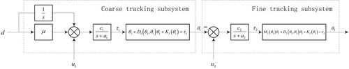
Let us consider a coarse-fine tracking system shown in Figure , the design objective is to attenuate (or decouple) the effect of the disturbance d, and let the final angle track a constant reference signal (which can be set to zero without loss of generality). The function of the coarse system is to acquisite the object and provide a ‘good’ input for the fine system.
Figure 1. The coarse-fine tracking system.
5.1. The HOFA model
According to Figure , the original model of the coarse tracking subsystem can be set up as
(91)
(91)
Taking differentials to the second equation in (Equation91
(91)
(91) ), gives
(92)
(92) Substituting the above Equation (Equation92
(92)
(92) ), together with the second equation in (Equation91
(91)
(91) ), into the first one in (Equation91
(91)
(91) ), yields the HOFA model for the coarse subsystem as
(93)
(93)
where
(94)
(94)
Parallelly, the original model for the fine tracking system is given by
(95)
(95)
Through a similar process, the HOFA model for the fine subsystem can be also obtained, as
(96)
(96)
where
(97)
(97)
with
(98)
(98)
Defining
(99)
(99)
and combining (Equation93
(93)
(93) ) and (Equation96
(96)
(96) ), give the following entire HOFA model for the whole system:
(100)
(100)
where
(101)
(101)
(102)
(102)
(103)
(103)
In the rest of this section, we assume
and
(104)
(104)
5.2. Disturbance attenuation
In this subsection, it is required that the effect of the disturbance d on the angle is as small as possible, thus the output equation is assumed to be
(105)
(105)
Therefore, the system to be considered is
(106)
(106)
where
is given by (Equation103
(103)
(103) ), and
(107)
(107)
The control law for system (Equation106
(106)
(106) ) is designed as
(108)
(108)
and the corresponding closed-loop system can be written as
(109)
(109)
which can be also written in the following state-space form:
(110)
(110)
where
(111)
(111)
5.2.1. Parameterisation of
Choose
(112)
(112)
where
and
. Then it follows from Theorem 3.4 that all the matrix
and the nonsingular matrix
satisfying
(113)
(113)
are given by
(114)
(114)
(115)
(115)
where
(116)
(116)
(117)
(117)
(118)
(118)
and
(119)
(119)
is a parameter matrix satisfying
(120)
(120)
5.2.2. Parameter optimisation
It follows from Theorem 3.5 that the norm of the transfer function
(121)
(121)
is given by
(122)
(122)
where
(123)
(123)
with
(124)
(124)
and the variables
and
are determined by
(125)
(125)
and
(126)
(126)
In order to give simultaneously a smaller control input, we also include the norm of the coefficient matrix
in the optimisation index, and this leads to the following index
(127)
(127)
where
and
are the selected weight factors. Solving the following optimisation problem
(128)
(128)
with
(129)
(129)
we obtain a sub-optimal solution as
(130)
(130)
and
(131)
(131)
Corresponding to these optimised values, the set of closed-loop poles are
(132)
(132)
and
(133)
(133)
5.2.3. Comparative simulation results
Let the initial values be taken as
(134)
(134)
(135)
(135)
In order to clearly see the effect of disturbance attenuation, we have take a large disturbance d as
(136)
(136)
Then the simulation of the system is carried out, and the results are shown in Figures and .
Figure 2. The regulated angles.
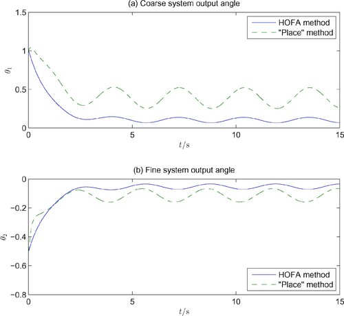
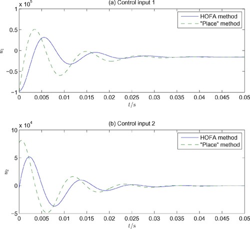
Figure 3. The control inputs.
In view of
(137)
(137)
pole assignment methods can be also applied to design the coefficient matrix
in the control law (Equation108
(108)
(108) ). For comparison, we also obtained another solution of
using the ‘place’ function. To make a fair comparison, the closed-loop poles are taken as in (Equation132
(132)
(132) ), and the gain matrix
is obtained as
(138)
(138)
Simulation corresponding to the above solution is also carried out, and the results are also shown in Figures and for comparison. It is clearly seen that the proposed approach is much more effective in the sense of disturbance attenuation and control effort consumption.
5.3. Asymptotic disturbance decoupling
In this subsection, the measurement output and the regulated output are assumed to be
(139)
(139)
and
(140)
(140)
respectively. These correspond to
(141)
(141)
Taking the above two output equations into consideration, we obtain the following HOFA system:
(142)
(142)
where
(143)
(143)
The disturbance d is assumed to be generated by the following exogenous system
(144)
(144)
with
(145)
(145)
5.3.1. Design of Π and Γ
According to Theorem 4.3, a parametric expression of the matrices Π and Γ in the control law (Equation59(59)
(59) ) can be given by
(146)
(146)
with the real parameter matrix
(147)
(147)
satisfying
(148)
(148)
Solving the above constraint (Equation148
(148)
(148) ), gives
(149)
(149)
thus Z can be taken as
(150)
(150)
Substituting (Equation150
(150)
(150) ) into (Equation146
(146)
(146) ), gives
(151)
(151)
5.3.2. Other parameters
A general parametric solution of the matrix is given by (Equation60
(60)
(60) ). For simplicity, here only a specific solution is given, as
(152)
(152)
where
(153)
(153)
(154)
(154)
The corresponding set of eigenvalues is
(155)
(155)
The parametric solutions of the gain matrices
and
can be obtained using Theorem 4.5. Again, for simplicity only a specific pair of solutions are given, as follows:
(156)
(156)
(157)
(157)
In such a case, the set of eigenvalues of
is
(158)
(158)
5.3.3. Simulation results
According to Theorem 4.3, the control law is finally designed as
(159)
(159)
where Π and Γ are given by (Equation151
(151)
(151) ),
is given by (Equation152
(152)
(152) ) – (Equation154
(154)
(154) ), and
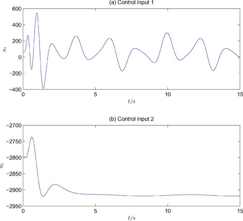
and
are given by (Equation156
(156)
(156) ) and (Equation157
(157)
(157) ), respectively.
When the initial values of the angles are taken as
(160)
(160)
with other system initial values being zeros, simulation results are carried out and shown in Figures and . It is clearly seen that
approaches to zero with a quite accurate precision in spite of the big sine disturbance. The magnitudes of the control inputs are relatively large because they need to take the burden to cancel the big nonlinearities in the system.
Figure 4. The regulated angles.
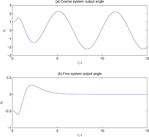
Figure 5. The control inputs.
6. Conclusion
In a wide sense, the problem of automatic control is to realise disturbance rejection. Disturbance rejection has remained a long-standing difficult problem in control systems design. Particularly, for nonlinear systems the problem appears even harder, since it heavily depends on the stabilisation of the systems, while it is well-known that, for many nonlinear systems, global stabilisation can be seldom achieved with the commonly used state-space model representation of the dynamical systems.
It has been shown in this series of papers that many dynamical control systems can be represented by a HOFA model. It is demonstrated in this paper that, with the proposed HOFA approaches, the problems of disturbance attenuation and decoupling in a nonlinear system can be conveniently converted into corresponding ones in a linear system. Based on this great feature, parametric approaches for disturbance attenuation and decoupling in nonlinear systems are easily proposed.
For disturbance attenuation, it is shown that a parametric state feedback controller exists, with which the norm of the disturbance-to-output transfer function of the closed-loop system can be also established and hence minimised. For asymptotic disturbance decoupling, it is shown that a parametric solution can be well-established by using complete parametric solutions to a type of homogeneous and nonhomogeneous generalised Sylvester matrix equations.
The proposed results and methodology can be further generalised in several directions. Particularly, disturbance compensation based on disturbance estimators is also worth investigation, disturbance rejection problems for discrete-time systems and time-delay systems can be also similarly treated. Like the treatment in Parts III and IV of the series, method of high-order backstepping can be also proposed for high-order strict-feedback systems with disturbances. Furthermore, disturbance rejection in sub-fully actuated systems certainly remains to be a very important future research topic.
Acknowledgments
The author is grateful to his Ph.D. students Guangtai Tian, Qin Zhao, Xiubo Wang, Weizhen Liu, Kaixin Cui, etc., for helping him with reference selection and proofreading. His particular thanks go to his student Tianyi Zhao for helping him working out the example.
Disclosure statement
No potential conflict of interest was reported by the author(s).
Additional information
Funding
Notes on contributors
Guangren Duan
Guangren Duan received his Ph.D. degree in Control Systems Sciences from Harbin Institute of Technology, Harbin, P. R. China, in 1989. After a two-year post-doctoral experince at the same university, he became professor of control systems theory at that university in 1991. He is the founder and currently the Director of the Center for Control Theory and Guidance Technology at Harbin Institute of Technology. He visited the University of Hull, the University of Sheffield, and also the Queen's University of Belfast, UK, from December 1996 to October 2002, and has served as Member of the Science and Technology committee of the Chinese Ministry of Education, Vice President of the Control Theory and Applications Committee, Chinese Association of Automation (CAA), and Associate Editors of a few international journals. He is currently an Academician of the Chinese Academy of sciences, and Fellow of CAA, IEEE and IET. His main research interests include parametric control systems design, nonlinear systems, descriptor systems, spacecraft control and magnetic bearing control. He is the author and co-author of 5 books and over 270 SCI indexed publications.
References
- Andiarti, R., & Moog, C. H. (1996). Output feedback disturbance decoupling in nonlinear systems. IEEE Transactions on Automatic Control, 41(11), 1683–1689. https://doi.org/https://doi.org/10.1109/9.544009
- Ball, J. A., Helton, J. W., & Walker, M. L. (1993). H∞ control for nonlinear-systems with output-feedback. IEEE Transactions on Automatic Control, 38(4), 546–559. https://doi.org/https://doi.org/10.1109/9.250523
- Duan, G. R. (1992a). Simple algorithm for robust pole assignment in linear output feedback. IEE Proceedings D Control Theory and Applications, 139(5), 465–470. https://doi.org/https://doi.org/10.1049/ip-d.1992.0058
- Duan, G. R. (1992b). Solution to matrix equation AV+BW=EV F and eigenstructure assignment for descriptor systems. Automatica, 28(3), 639–642. https://doi.org/https://doi.org/10.1016/0005-1098(92)90191-H
- Duan, G. R. (1993a). Solutions of the equation AV + BW = V F and their application to eigenstructure assignment in linear-systems. IEEE Transactions on Automatic Control, 38(2), 276–280. https://doi.org/https://doi.org/10.1109/9.250470
- Duan, G. R. (1993b). Robust eigenstructure assignment via dynamical compensators. Automatica, 29(2), 469–474. https://doi.org/https://doi.org/10.1016/0005-1098(93)90140-O
- Duan, G. R. (1998). Eigenstructure assignment and response analysis in descriptor linear systems with state feedback control. International Journal of Control, 69(5), 663–694. https://doi.org/https://doi.org/10.1080/002071798222622
- Duan, G. R. (2004). Parametric eigenstructure assignment in second-order descriptor linear systems. IEEE Transactions on Automatic Control, 49(10), 1789–1795. https://doi.org/https://doi.org/10.1109/TAC.2004.835580
- Duan, G. R. (2005). Parametric approaches for eigenstructure assignment in high-order linear systems. International Journal of Control Automation and Systems, 3(3), 419–429.
- Duan, G. R. (2015). Generalized Sylvester equations: Unified parametric solutions. CRC Press.
- Duan, G. R. (2020a). High-order fully actuated system approaches: Part I. Models and basic procedure. International Journal of System Sciences. https://doi.org/https://doi.org/10.1080/00207721.2020.1829167
- Duan, G. R. (2020b). High-order fully actuated system approaches: Part II. Generalized strict-feedback systems. International Journal of System Sciences. https://doi.org/https://doi.org/10.1080/00207721.2020.1829168
- Duan, G. R. (2020c). High-order fully actuated system approaches: Part III. Robust control and high-order backstepping. International Journal of System Sciences. https://doi.org/https://doi.org/10.1080/00207721.2020.1849863
- Duan, G. R. (2020d). High-order fully actuated system approaches: Part IV. Adaptive control and high-order backstepping. International Journal of System Sciences. https://doi.org/https://doi.org/10.1080/00207721.2020.1849864
- Duan, G. R. (2021a). High-order system approaches: I. Full-actuation and parametric design. Acta Automatica Sinica, 46(7), 1333–1345 (in Chinese). https://doi.org/https://doi.org/10.1080/00207721.2020.1829167
- Duan, G. R. (2021b). High-order system approaches: II. Controllability and fully-actuation. Acta Automatica Sinica, 46(8), 1571–1581 (in Chinese). https://doi.org/https://doi.org/10.16383/j.aas.c200369
- Duan, G. R. (2021c). High-order system approaches: III. observability and observer design. Acta Automatica Sinica, 46(9), 1885–1895 (in Chinese). https://doi.org/https://doi.org/10.1080/00207721.2020.1849863
- Duan, G. R. (2021d). High-order fully actuated system approaches: Part V. Robust adaptive control. International Journal of System Sciences.
- Duan, G. R. (2021e). HOFA system approaches: VII. Controllability, stabilizability and parametric designs. International Journal of System Sciences.
- Duan, G. R., & Huang, L. (2006). Disturbance attenuation in model following designs of a class of second-order systems: A parametric approach. In 2006 SICE-ICASE international joint conference, Busan, South Korea (pp. 5662–5667). IEEE Press.
- Duan, G. R., Irwin, G. W., & Liu, G. P. (2002). Disturbance attenuation in linear systems via dynamical compensators: A parametric eigenstructure assignment approach. IEE Proceedings – Control Theory and Applications, 147(2), 129–136. https://doi.org/https://doi.org/10.1049/ip-cta:20000135
- Duan, G. R., Liu, G. P., & Thompson, S. (2000a). Disturbance attenuation in Luenberger function observer designs: A parametric approach. IFAC Proceedings Volumes, 33(14), 41–46. https://doi.org/https://doi.org/10.1016/S1474-6670(17)36202-X
- Duan, G. R., Liu, G. P., & Thompson, S. (2000b). Disturbance decoupling in descriptor systems via output feedback: A parametric eigenstructure assignment approach. In Proceedings of the 39th IEEE conference on decision and control, Sydney, NSW (pp. 3660–3665). IEEE Press.
- Duan, G. R., Patton, R. J., Chen, J., & Chen, Z. (1997). A parametric approach for robust fault detection in linear systems with unknown disturbances. IFAC Proceedings Volumes, 30(18), 307–311. https://doi.org/https://doi.org/10.1016/S1474-6670(17)42419-0
- Duan, G. R., & Yu, H. H. (2013). LMIs in control systems: Analysis, design and applications. CRC Press.
- Duan, G. R., & Zhao, T. Y. (2020). Observer-based multi-objective parametric design for spacecraft with super flexible netted antennas. Science China Information Sciences, 63(7), 172002. https://doi.org/https://doi.org/10.1007/s11432-020-2916-8
- Doyle, J. C., Zhou, K., Glover, K., & Bodenheimer, B. (1994). Mixed H2 and performance objectives II: Optimal control. IEEE Transactions on Automatic Control, 39(8), 1575–1587. https://doi.org/https://doi.org/10.1109/9.310031
- Gao, Z. (2014). On the centrality of disturbance rejection in automatic control. ISA Transactions, 53(4), 850–857. https://doi.org/https://doi.org/10.1016/j.isatra.2013.09.012
- Huang, J. (1995). Asymptotic tracking and disturbance rejection in uncertain nonlinear systems. IEEE Transactions on Automatic Control, 40(6), 1118–1122. https://doi.org/https://doi.org/10.1109/9.388697
- Huang, L., Wei, Y. Y., & Duan, G. R. (2006). Disturbance attenuation in model following designs: A parametric approach. In 2006 Chinese control conference, Harbin, China (pp. 812–815). IEEE Press.
- Huang, Y., & Xue, W. C. (2014). Active disturbance rejection control: Methodology and theoretical analysis. ISA Transactions, 53(4), 963–976. https://doi.org/https://doi.org/10.1016/j.isatra.2014.03.003
- Huijberts, H. J. C., Nijmeijer, H., & van der wegen, L. L. M. (1992). Dynamic disturbance decoupling for nonlinear systems. SIAM Journal on Control and Optimization, 30(2), 336–349. https://doi.org/https://doi.org/10.1137/0330021
- Isidori, A., & Astolfi, A. (1992). Disturbance attenuation and Hinfty-control via measurement feedback in nonlinear-systems. IEEE Transactions on Automatic Control, 37(9), 1283–1293. https://doi.org/https://doi.org/10.1109/9.159566
- Jayawardhana, B., & Weiss, G. (2008). Tracking and disturbance rejection for fully actuated mechanical systems. Automatica, 44(11), 2863–2868. https://doi.org/https://doi.org/10.1016/j.automatica.2008.03.030
- Kaldmae, A., Kotta, U., Shumsky, A., & Zhirabok, A. (2013). Measurement feedback disturbance decoupling in discrete-time nonlinear systems. Automatica, 49(9), 2887–2891. https://doi.org/https://doi.org/10.1016/j.automatica.2013.06.013
- Kaldmae, A., Kotta, U., Shumsky, A., & Zhirabok, A. (2018). Disturbance decoupling in nonlinear hybrid systems. Nonlinear Analysis: Hybrid Systems, 28(2), 42–53. https://doi.org/https://doi.org/10.1016/j.nahs.2017.11.001
- Liu, X. P., Jutan, A., & Rohani, S. (2004). Almost disturbance decoupling of MIMO nonlinear systems and application to chemical processes. Automatica, 40(3), 465–471. https://doi.org/https://doi.org/10.1016/j.automatica.2003.10.019
- Marino, R., Respondek, W., & van der Schaft, A. J. (1989). Almost disturbance decoupling for single-input single-output nonlinear systems. IEEE Transactions on Automatic Control, 34(9), 1013–1017. https://doi.org/https://doi.org/10.1109/9.35821
- Marino, R., & Tomei, P. (2000). Adaptive output feedback tracking with almost disturbance decoupling for a class of nonlinear systems. Automatica, 36(12), 1871–1877. https://doi.org/https://doi.org/10.1016/S0005-1098(00)00109-6
- Marino, R., & Tomei, P. (2005). Adaptive tracking and disturbance rejection for uncertain nonlinear systems. IEEE Transactions on Automatic Control, 50(1), 90–95. https://doi.org/https://doi.org/10.1109/TAC.2004.841132
- Moog, C. H., Castro-Linares, R., Velasco-Villa, M., & Marquez-Martinez, L. A. (2000). The disturbance decoupling problem for time-delay nonlinear systems. IEEE Transactions on Automatic Control, 45(2), 305–309. https://doi.org/https://doi.org/10.1109/9.839954
- Qian, C. J., & Lin, W. (2000). Almost disturbance decoupling for a class of high-order nonlinear systems. IEEE Transactions on Automatic Control, 45(6), 1208–1214. https://doi.org/https://doi.org/10.1109/9.863608
- Ran, M. P., Wang, Q., Dong, C. Y., & Xie, L. H. (2020). Active disturbance rejection control for uncertain time-delay nonlinear systems. Automatica, 112(18), 108692. https://doi.org/https://doi.org/10.1016/j.automatica.2019.108692
- Saberi, A, Stoorvogel, A. A., & Sannuti, P. (2000). Control of linear systems with regulation and input constraints. Springer.
- Sun, Z. Y., Zhang, C. H., & Wang, Z. (2017). Adaptive disturbance attenuation for generalized high-order uncertain nonlinear systems. Automatica, 80, 102–109. https://doi.org/https://doi.org/10.1016/j.automatica.2017.02.036
- Velasco, M., Alvarez, J. A., & Castro, R. (1997). Disturbance decoupling for time delay systems. International Journal of Robust and Nonlinear Control, 7(9), 847–864. https://doi.org/https://doi.org/10.1002/(ISSN)1099-1239
- Wang, Z. D., Ho, D. W. C., Liu, Y. R., & Liu, X. H. (2009). Robust H∞ control for a class of nonlinear discrete time-delay stochastic systems with missing measurements. Automatica, 45(3), 684–691. https://doi.org/https://doi.org/10.1016/j.automatica.2008.10.025
- Wang, Z. D., Shen, B., Shu, H. S., & Wei, G. L. (2012). Quantized H∞ control for nonlinear stochastic time-delay systems with missing measurements. IEEE Transactions on Automatic Control, 57(6), 1431–1444. https://doi.org/https://doi.org/10.1109/TAC.2011.2176362
- Zheng, L., Cheng, D., & Li, C. (2005). Disturbance decoupling of switched nonlinear systems. IEE Proceedings - Control Theory and Applications, 152(1), 49–54. https://doi.org/https://doi.org/10.1049/ip-cta:20051120
- Zhou, K., Glover, K., Bodenheimer, B., & Doyle, J. C. (1994). Mixed H2 and H∞ performance objectives: I. Robust performance analysis. IEEE Transactions on Automatic Control, 39(8), 1564–1574. https://doi.org/https://doi.org/10.1109/9.310030