High-order fully actuated system approaches: part VII. Controllability, stabilisability and parametric designs

Abstract

In this paper, high-order fully actuated (HOFA) models with multiple orders for general dynamical control systems are firstly proposed, for which controllers can be easily designed such that the closed-loop systems are constant linear ones with completely assignable eigenstructures. Based on this special feature of the type of HOFA models, controllability of general dynamical control systems is proposed. It is revealed that a general dynamical control system can be represented by a controllable subsystem described by a HOFA model, and an extra uncontrollable one or supplementary one. While a general dynamical control system is called stabilisable if its uncontrollable (autonomous) subsystem does not exist, or is stable in a certain sense. Finally, two parametric design approaches for control of the type of general HOFA models are proposed, which provide all the design degrees of freedom. Several examples, including ones of sub-fully actuated systems, are treated, which demonstrate the effect of the proposed theories.

Keywords:

• High-order fully actuated systems
• controllability
• stabilisability
• parametric designs
• eigenstructure assignment

1. Introduction

Controllability reflects the nature of a dynamical control system, and is a very important issue in control system analysis.

1.1. Problems related to controllability

Controllability analysis for linear control systems is mature, and the results are neat and elegant. While for controllability analysis in nonlinear control systems, the results are far from satisfactory.

Firstly, for linear systems, the concept of controllability is clear and unique, while for nonlinear systems, there are many definitions, such as global controllability (Klamka, 1975b; Mirza & Womack, 1972; Vidyasag, 1972), local controllability (Klamka, 1975a), relative controllability (Klamka, 1976), closed controllability (Sun, 2010), strong controllability and weak controllability (Chen & Qin, 1987), vibrational controllability (Bellman et al., 1986), norm-controllability (Müller et al., 2015), N-step controllability and asymptotical controllability (Clarke et al., 1997; Hanba, 2017). Some of these definitions are proposed for the various special types of nonlinear systems according to one's needs.

Secondly, for relative general nonlinear systems, controllability seems to be a problem that never deserves a necessary and sufficient condition. Existing necessary and sufficient conditions for controllability are only obtained for certain very special types of systems, e.g. systems with strict symmetry structure (Jing & Hu, 1996), special bilinear systems (Tie et al., 2011), two-dimensional affine systems (Sun, 2007), triangular systems (Celikovsky, 2000; Celikovsky & Nijmeijer, 1997), and single-input systems (Zheng et al., 2001).

Thirdly, for controllability analysis in nonlinear systems, too much abstract mathematics is used, for instance, the Lie algebra, differential geometry, manifold theory, and field theory. Of course, there is nothing wrong, but encouraged, to apply profound mathematics to solve scientific problems, but with most of such work on controllability analysis of nonlinear systems, not only the intermediate deduction steps, but also the final results are presented in terms of such abstract and profound mathematical terminologies and notations. Such results by no means can be used by the majority of the control theory community, not to say the group of control engineers.

Fourthly, the concept of controllability is only defined for systems described by state-space models, because it is defined based on the concept of state vectors of state-space systems. What is more, this concept is kept within the closed frame of the state-space approaches, and can not be generalised to suit systems in other forms. Take a linear system in an input–output representation for example. It is well-known that such a system has a state-space realisation, and it is natural to define the controllability of a linear system in an input–output form via its state-space realisations. However, the problem is that, the system may have on one hand a controllable realisation, while on the other hand an uncontrollable realisation. This clearly gives an ambiguity. If minimal realisations of the systems were used to define the controllability of such systems, then all systems would be controllable since all minimal realisations are controllable. In this case there would not be the need of defining. This is certainly a problem since, to our general understanding, any control system in whatever form should deserve a concept of controllability.

Fifthly, it is expected that controllability analysis helps control systems design, as it is in the case of linear systems. While for nonlinear control systems, certain concepts of controllability along the traditional Kalman stream may not help the design. Such a fact is discovered by R. W. Brocket as early as 1983. More specifically, it is put in Brocket (1983), ‘Whereas it might have been suspected that controllability would insure the existence of a stabilising control law, Theorem 1 uses a degree-theoretic argument to show this is far from being the case'. Additionally, Brocket (1983) also ‘provides a counter example to the oft repeated conjecture asserting that a reasonable form of local controllability implies the existence of a stabilizing control law’. Do these facts lead us to suspect whether some of these concepts of controllability are defined properly?

1.2. Reasons

To conclude, for nonlinear systems the various concepts of controllability in the state-space mainstream are generally not working well enough. Based on a thorough review of the results on nonlinear systems theory, Casti (1982) made the following statements:

All current indications point toward the conclusion that seeking a completely general theory of nonlinear systems is somewhat akin to the search for the Holy Grail: a relatively harmless activity full of many pleasant surprises and mild disappointments, but ultimately unrewarding.

While as a matter of fact, among all aspects of progresses in nonlinear systems theory, controllability analysis is the least. By now 40 years have past, on controllability of nonlinear control systems, there have not been much essential advances.

Then here is the question, why is it the case?

The answer would be generally that nonlinear systems are too complicated and the state of this art has just reflected what it should be. But is the direction right?

Controllability was originally defined by Kalman (1960) (see, also Kalman, 1959), and today's various definitions of controllability, although vary in certain ways, are still following the same line of that given by Kalman. The concept is defined, in nature, using the solution (response) of the system. For linear systems, we have an elegant formula for the state response. As a consequence, beautiful results for controllability of linear systems are proposed. However, for a nonlinear system, it is impossible to give explicit analytical closed-form solutions for the system states, and this naturally prevents us from obtaining general useful and meaningful criteria for controllability of nonlinear systems.

Based on the Kalman-like definitions of controllability in the state-space framework, essential advances in controllability analysis of nonlinear control systems await further breakthroughs in analytical solutions of general nonlinear differential equations. While the latter seems no time to come due to its well-recognised difficulty. Filled with disappointments, Casti (1982) suggested that ‘A far more profitable path to follow is to concentrate upon special classes of nonlinear problems, usually motivated by applications, and to use the structure inherent in these classes as a guide to useful (i.e. applicable) results'. In short, it is in vain to attempt proposing relatively general nonlinear control systems theories. Such a point was well accepted, so no wonder most of the results today on nonlinear systems theory are focused on special types of systems.

State-space approaches for control systems analysis and designs were formally proposed by Kalman (1960). While the idea can really be traced back to 1750, when Euler invented the variable extension method for solving high-order differential equations by converting the equation into a first-order one (Klein, 1990). The problem solved then is really today's problem of state response analysis.

State-space models concentrate on the state vectors, and are originally helpful to state solutions, as early demonstrated by Euler. In today's control systems theory, they are also effective and convenient to handle problems closely related with the state vector, such as state observers designs, and state filtering and smoothing. However, for problems of controller designs, the state-space models may not provide much convenience, and hence may not be the best choice. Following the lead of Kalman (1960), control scientists in the past half century have naturally adopted the state-space approaches to investigate controllability analysis, together with most of the other nonlinear control problems. However, since controllability is a problem very closely related to the problem of control, we might wonder if state-space approaches are the right methodology for controllability analysis?

1.3. Fully actuated system approaches

Physically, a fully actuated system is regarded to be a second-order mechanical system, which has a control actuator for each freedom. For such a system, a controller can be easily designed to cancel the nonlinearities in the system and thus results in a constant linear closed-loop system (Duan, 2020a, 2021a). Unfortunately, this set of fully actuated systems, although possess such a superior advantage, have not attracted much attention of the control scientists, since they are generally considered to be only a small minority of control systems.

Very recently, it was discovered that the physical concept of full actuation can be mathematically generalised to describe a variety of control systems, and most under actuated systems can also be converted into fully actuated ones. Particularly, it has been proven that, linear controllable systems (Duan, 2020b), feedback linearisable systems (Duan, 2020a), strict-feedback systems (Duan, 2020a, 2021b), and some other more general type of nonlinear systems (Duan, 2021a), can all be converted equivalently into high-order fully actuated (HOFA) systems. This discovery motivates the very effective and simple HOFA approaches for control systems analysis and design. Now in this present paper, a different but more meaningful form of general HOFA systems is proposed and investigated.

With a HOFA model, as in the case of second-order mechanical systems, a controller can be easily designed such that a linear closed-loop system with a completely assignable eigenstructure is obtained. Such a phenomenon, in essence, fully represents the meaning of controllability. Based on this phenomenon, controllability of a general nonlinear system is proposed in Duan (2020b). In this present paper, the concept of controllability is further modified to suit the general system case. Meantime, by proposing the uncontrollable subsystem and the supplementary subsystem, stabilisability and strong stabilisability of a general nonlinear system are also defined. According to the proposed theory, any nonlinear system can be modelled by a controllable subsystem represented by a HOFA model, together with an extra uncontrollable one (if exists) or a supplementary one (if exists). Based on this structure, a nonlinear system is defined to be stabilisable if its uncontrollable subsystem does not exist or is stable in a certain sense, and is defined to be strongly stabilisable if a system composed of a HOFA subsystem and a supplementary subsystem is stabilisable in a certain sense by a linearising controller designed only for the HOFA subsystem.

Parallel to the last part in Duan (2021a), two complete parametric designs of the newly proposed HOFA model are presented. One is the decoupled design, and the other is the coupled one. In both designs, a controller is constructed such that the closed-loop system is a constant linear one with an arbitrarily assignable eigenstructure. General parametric forms for the designed feedback controller as well as the closed-loop system are established. The degrees of freedom existing in both designs are also calculated.

In the sequential sections, $I_n$ denotes the identity matrix, $\varnothing$ denotes the null set, and $\mathrm{\Omega }\mathrm{\setminus }\mathrm{\Theta }$ represents the complement of the set Θ in set Ω. Furthermore, $det\left(A\right)$ and $\mathrm{a}\mathrm{d}\mathrm{j}\left(A\right)$ denote the determinant and the adjoint matrix of a matrix A, respectively. For $x,x_i\in {\mathbb{R}}^m,$ and $A_i\in {\mathbb{R}}^{m\times m},$ $n_0,n_i\in \mathbb{N},n_0<n_i,$ $i=1,2,\dots ,n,$ as in Duan (2021c), the following symbols are used in the paper: $\begin{array}{rl}& x^{(n_1\sim n_2)}=\left[\begin{array}{c}{x}^{\left(n_1\right)}\\ x^{\left(n_1+1\right)}\\ ⋮\\ x^{\left(n_2\right)}\end{array}\right],n_1\le n_2,\\ & x_{i\sim j}^{(n_1\sim n_2)}=\left[\begin{array}{c}{x}_i^{(n_1\sim n_2)}\\ x_{i+1}^{(n_1\sim n_2)}\\ ⋮\\ x_j^{(n_1\sim n_2)}\end{array}\right],i\le j,n_1\le n_2,\\ & x_k^{\left(n_k\right)}{|}_{k=i\sim j}=\left[\begin{array}{c}{x}_i^{\left(n_i\right)}\\ x_{i+1}^{\left(n_{i+1}\right)}\\ ⋮\\ x_j^{\left(n_j\right)}\end{array}\right],i\le j,\\ & x_k^{(n_0\sim n_k)}{|}_{k=i\sim j}=\left[\begin{array}{c}{x}_i^{(n_0\sim n_i)}\\ x_{i+1}^{(n_0\sim n_{i+1})}\\ ⋮\\ x_j^{(n_0\sim n_j)}\end{array}\right],j\ge i,\\ & A_{0\sim n-1}=\left[\begin{array}{cccc}{A}_0& A_1& \cdots & A_{n-1}\end{array}\right],\\ & \mathrm{\Phi }\left(A_{0\sim n-1}\right)=\left[\begin{array}{cccc}0& I& & \\ & & \ddots & \\ & & & I\\ -A_0& -A_1& \cdots & -A_{n-1}\end{array}\right].\end{array}$The paper is organised into seven sections. In the next section, more general HOFA models of dynamical control systems are introduced and investigated, and in Sections 3 and 4, the concepts of controllability and stabilisability of general dynamical control systems are proposed, respectively. Section 5 further presents two parametric design approaches for the proposed general HOFA models. Two examples are further presented in Section 6, followed by a brief concluding remark in Section 7.

2. General HOFA models

In Duan (2020a) (see also Duan, 2021a), a type of HOFA models are proposed in the following form (1) $E{x}^{\left(n\right)}=f(x^{(0\sim n-1)},\zeta )+B(x^{(0\sim n-1)},\zeta )u,$(1) where $n\ge 1$ is an integer, x and $u\in {\mathbb{R}}^r$ are the state vector and the system input vector, respectively, $\zeta \in {\mathbb{R}}^p$ is an external vector, $E\in {\mathbb{R}}^{r\times r}$ is a constant matrix, which is usually the identity matrix, but may be sometimes singular, $f(x^{(0\sim n-1)},\zeta )\in {\mathbb{R}}^r$ is a sufficiently differentiable vector function, and $B(x^{(0\sim n-1)},\zeta )\in {\mathbb{R}}^{r\times r}$ is a matrix function. When $B(x^{(0\sim n-1)},\zeta )$ is nonsingular for all $\zeta \in {\mathbb{R}}^p,t\ge 0,$ and $x^{\left(i\right)}\in {\mathrm{\Omega }}_i\subset {\mathbb{R}}^r,i=0,1,\dots ,n-1$, the above system (1(1) $E{x}^{\left(n\right)}=f(x^{(0\sim n-1)},\zeta )+B(x^{(0\sim n-1)},\zeta )u,$(1) ) is called fully actuated on $\mathrm{\Omega }={\mathrm{\Omega }}_0\times {\mathrm{\Omega }}_1\times \cdots \times {\mathrm{\Omega }}_{n-1}.$ In the case of ${\mathrm{\Omega }}_i={\mathbb{R}}^r,i=0,1,\dots ,n-1$, the system (1(1) $E{x}^{\left(n\right)}=f(x^{(0\sim n-1)},\zeta )+B(x^{(0\sim n-1)},\zeta )u,$(1) ) is called (globally) fully actuated (Duan, 2020b).

Clearly, the HOFA system (1(1) $E{x}^{\left(n\right)}=f(x^{(0\sim n-1)},\zeta )+B(x^{(0\sim n-1)},\zeta )u,$(1) ) appears in a descriptor system form. In this section, let us propose a different but more meaningful description of HOFA systems.

2.1. Motivations

Before presenting the new form of general HOFA models with multiple orders, let us first mention two aspects of motivations for proposing the general form.

2.1.1. The linear system case

Consider a linear system in the following state-space form (2) $\dot{x}=Ax+Bu,$(2) where $x\in {\mathbb{R}}^n$ and $u\in {\mathbb{R}}^r$ are the state vector and input vector, respectively, and $A\in {\mathbb{R}}^{n\times n},$ and $B\in {\mathbb{R}}^{n\times r}$ are the coefficient matrices. It is proven in Duan (2020b) (see Theorem 2 therein) that the linear system (2(2) $\dot{x}=Ax+Bu,$(2) ) is controllable if and only if it can be equivalently converted into a linear HOFA system in the form of (3) $A_{\mu }{z}^{\left(\mu \right)}+A_{\mu -1}{z}^{\left(\mu -1\right)}+\cdots A_1\dot{z}+A_{0}z=\tilde{B}u,$(3) where z is a vector of r dimension, $A_i\in {\mathbb{R}}^{r\times r},\text{ı}=0,1,\dots ,\mu ,$ are the coefficient matrices, and (4) $\tilde{B}=\left[\begin{array}{ccccc}1& b_{12}& b_{13}& \cdots & b_{1r}\\ 0& 1& b_{23}& \cdots & b_{2r}\\ 0& 0& 1& \cdots & b_{3r}\\ ⋮& ⋮& ⋮& \ddots & ⋮\\ 0& 0& 0& \cdots & 1\end{array}\right].$(4) Since some of the matrices $A_i,$ and particularly $A_{\mu },$ may be singular, the above system (3(3) $A_{\mu }{z}^{\left(\mu \right)}+A_{\mu -1}{z}^{\left(\mu -1\right)}+\cdots A_1\dot{z}+A_{0}z=\tilde{B}u,$(3) ) can be generally written in the following form: (5) $\left[\begin{array}{c}{x}_1^{\left({\mu }_1\right)}\\ x_2^{\left({\mu }_2\right)}\\ ⋮\\ x_{\eta }^{\left({\mu }_{\eta }\right)}\end{array}\right]=\left[\begin{array}{c}{L}_1\left(x_k^{\left(0\sim {\mu }_k-1\right)}{|}_{k=1\sim \eta }\right)\\ L_2\left(x_k^{\left(0\sim {\mu }_k-1\right)}{|}_{k=1\sim \eta }\right)\\ ⋮\\ L_{\eta }\left(x_k^{\left(0\sim {\mu }_k-1\right)}{|}_{k=1\sim \eta }\right)\end{array}\right]+\hat{B}u,$(5) where ${\mu }_k,k=1,2,\dots ,\eta ,$ are a set of integers, $x_k,=1,2,\dots ,\eta ,$ are a set of vectors of proper dimensions, and $L_k(\cdot ),k=1,2,\dots ,\eta ,$ are a set of linear functions.

2.1.2. The nonlinear system case

In 1989, a controllability canonical form for a type of nonlinear systems was proposed in Li and Gao (1989). It is shown in Duan (2020b) that this controllability canonical form can be equivalently converted into a HOFA system in the form of (1(1) $E{x}^{\left(n\right)}=f(x^{(0\sim n-1)},\zeta )+B(x^{(0\sim n-1)},\zeta )u,$(1) ), while it can be discovered in the proof of Theorem 4 in Duan (2020b) that this canonical form is in fact equivalent to a system in the following form (6) $\left[\begin{array}{c}{x}_1^{\left({\mu }_1\right)}\\ x_2^{\left({\mu }_2\right)}\\ ⋮\\ x_{\eta }^{\left({\mu }_{\eta }\right)}\end{array}\right]=\left[\begin{array}{c}{f}_1\left(x_k^{\left(0\sim {\mu }_k-1\right)}{|}_{k=1\sim \eta },t\right)\\ f_2\left(x_k^{\left(0\sim {\mu }_k-1\right)}{|}_{k=1\sim \eta },t\right)\\ ⋮\\ f_{\eta }\left(x_k^{\left(0\sim {\mu }_k-1\right)}{|}_{k=1\sim \eta },t\right)\end{array}\right]+\hat{B}u,$(6) where $f_k(\cdot ),k=1,2,\dots ,\eta ,$ are a set of nonlinear functions.

Very recently, it is shown in Duan (2021a) that a relatively general type of nonlinear systems can be equivalently converted, under certain conditions, into the following form: (7) $\begin{array}{rl}\left[\begin{array}{c}{x}_1^{\left({\mu }_1\right)}\\ x_2^{\left({\mu }_2\right)}\end{array}\right]& =\left[\begin{array}{c}{f}_1\left(x_k^{\left(0\sim {\mu }_k-1\right)}{|}_{k=1\sim 2},t\right)\\ f_2\left(x_k^{\left(0\sim {\mu }_k-1\right)}{|}_{k=1\sim 2},t\right)\end{array}\right]\\ & +B\left(x_k^{\left(0\sim {\mu }_k-1\right)}{|}_{k=1\sim 2},t\right)u,\end{array}$(7) where $B(x_k^{(0\sim {\mu }_k-1)}{|}_{k=1\sim 2},t)$ is a nonsingular matrix for all $x_k^{(0\sim {\mu }_k-1)},k=1,2,$ and $t\ge 0.$

2.2. General HOFA models

Due to the above motivations, we can give the following general form of an affine HOFA model with multiple orders: (8) $\begin{array}{rl}\left[\begin{array}{c}{x}_1^{\left({\mu }_1\right)}\\ x_2^{\left({\mu }_2\right)}\\ ⋮\\ x_{\eta }^{\left({\mu }_{\eta }\right)}\end{array}\right]& =\left[\begin{array}{c}{f}_1\left(x_k^{\left(0\sim {\mu }_k-1\right)}{|}_{k=1\sim \eta },\zeta ,t\right)\\ f_2\left(x_k^{\left(0\sim {\mu }_k-1\right)}{|}_{k=1\sim \eta },\zeta ,t\right)\\ ⋮\\ f_{\eta }\left(x_k^{\left(0\sim {\mu }_k-1\right)}{|}_{k=1\sim \eta },\zeta ,t\right)\end{array}\right]\\ & +B\left(\cdot \right)u,\end{array}$(8) where $\zeta \in {\mathbb{R}}^p$ is an external vector, ${\mu }_k,=1,2,\dots ,\eta ,$ are a set of integers, $x_k\in {\mathbb{R}}^{r_k},k=1,2,\dots ,\eta ,$ are a set of vectors of proper dimensions, with $r_k,k=1,2,\dots ,\eta ,$ being a set of distinct integers satisfying (9) $r_1+r_2+\cdots +r_{\eta }=r.$(9) Further, $f_k(\cdot )\in {\mathbb{R}}^{r_k},k=1,2,\dots ,\eta ,$ are a set of nonlinear vector functions, and $B\left(\cdot \right)=B\left(x_k^{\left(0\sim {\mu }_k-1\right)}{|}_{k=1\sim \eta },\zeta ,t\right)\in {\mathbb{R}}^{r\times r}$is a nonlinear matrix function of $x_k^{(0\sim {\mu }_k-1)}{|}_{k=1\sim \eta },\zeta ,$ and t>0.

If we denote $\begin{array}{rl}& f\left(x_k^{\left(0\sim {\mu }_k-1\right)}{|}_{k=1\sim \eta },\zeta ,t\right)\\ & =\left[\begin{array}{c}{f}_1\left(x_k^{\left(0\sim {\mu }_k-1\right)}{|}_{k=1\sim \eta },\zeta ,t\right)\\ f_2\left(x_k^{\left(0\sim {\mu }_k-1\right)}{|}_{k=1\sim \eta },\zeta ,t\right)\\ ⋮\\ f_{\eta }\left(x_k^{\left(0\sim {\mu }_k-1\right)}{|}_{k=1\sim \eta },\zeta ,t\right)\end{array}\right],\end{array}$then the HOFA system can be compactly written as (10) $x_k^{\left({\mu }_k\right)}{|}_{k=1\sim \eta }=f\left(x_k^{\left(0\sim {\mu }_k-1\right)}{|}_{k=1\sim \eta },\zeta ,t\right)+B\left(\cdot \right)u.$(10) Clearly, in the case of $\eta =1$, the above HOFA model (8(8) $\begin{array}{rl}\left[\begin{array}{c}{x}_1^{\left({\mu }_1\right)}\\ x_2^{\left({\mu }_2\right)}\\ ⋮\\ x_{\eta }^{\left({\mu }_{\eta }\right)}\end{array}\right]& =\left[\begin{array}{c}{f}_1\left(x_k^{\left(0\sim {\mu }_k-1\right)}{|}_{k=1\sim \eta },\zeta ,t\right)\\ f_2\left(x_k^{\left(0\sim {\mu }_k-1\right)}{|}_{k=1\sim \eta },\zeta ,t\right)\\ ⋮\\ f_{\eta }\left(x_k^{\left(0\sim {\mu }_k-1\right)}{|}_{k=1\sim \eta },\zeta ,t\right)\end{array}\right]\\ & +B\left(\cdot \right)u,\end{array}$(8) ), or (10(10) $x_k^{\left({\mu }_k\right)}{|}_{k=1\sim \eta }=f\left(x_k^{\left(0\sim {\mu }_k-1\right)}{|}_{k=1\sim \eta },\zeta ,t\right)+B\left(\cdot \right)u.$(10) ), reduces to the form of (1(1) $E{x}^{\left(n\right)}=f(x^{(0\sim n-1)},\zeta )+B(x^{(0\sim n-1)},\zeta )u,$(1) ) with E = I, which is proposed in Duan (2020a) (see, also Duan, 2021a). When nonlinear uncertainties, unknown parameters and disturbances are added to this basic HOFA model, robust and adaptive control as well as disturbance rejection control have been investigated in Duan (2020d, 2020e, 2021c, 2021d).

Let ${\mathrm{\Omega }}_{ki}\subset {\mathbb{R}}^{r_k},i=0,1,\dots ,{\mu }_k-1,$ $k=1,2,\dots ,\eta$, be a set of open sets, and define (11) $\left\{\begin{array}{l}{\mathrm{\Omega }}_k={\mathrm{\Omega }}_{k0}\times {\mathrm{\Omega }}_{k1}\times \cdots \times {\mathrm{\Omega }}_{k,{\mu }_k-1}\subset {\mathbb{R}}^{r_k{\mu }_k}\\ \mathrm{\Omega }={\mathrm{\Omega }}_0\times {\mathrm{\Omega }}_1\times \cdots \times {\mathrm{\Omega }}_{\eta }\subset {\mathbb{R}}^{\varkappa },\end{array}\right.$(11) where (12) $\varkappa =\sum _{i=1}^{\eta }{r}_k{\mu }_k.$(12) Then the following three relations are obviously equivalent:

1. $x_k^{\left(i\right)}\in {\mathrm{\Omega }}_{ki}\subset {\mathbb{R}}^{r_k},\text{ı}=0,1,\dots ,{\mu }_k-1,k=1,2,\dots ,\eta ;$

2. $x_k^{(0\sim {\mu }_k-1)}\in {\mathrm{\Omega }}_k\subset {\mathbb{R}}^{r_k{\mu }_k},k=1,2,\dots ,\eta$; and

3. $x_k^{(0\sim {\mu }_k-1)}{|}_{k=1\sim \eta }\in \mathrm{\Omega }\subset {\mathbb{R}}^{\varkappa }.$

With the above preparation, let us introduce the following definition.

Definition 2.1

If $x_k^{(0\sim {\mu }_k-1)}{|}_{k=1\sim \eta }\in {\mathbb{R}}^{\varkappa }$ satisfies (13) $\begin{array}{rl}& detB\left(x_k^{\left(0\sim {\mu }_k-1\right)}{|}_{k=1\sim \eta },\zeta ,t\right)=0\text{ or }\mathrm{\infty },\\ & \mathrm{\exists }\zeta \in {\mathbb{R}}^p,t\ge 0,\end{array}$(13) then it is called a singular point of system (8(8) $\begin{array}{rl}\left[\begin{array}{c}{x}_1^{\left({\mu }_1\right)}\\ x_2^{\left({\mu }_2\right)}\\ ⋮\\ x_{\eta }^{\left({\mu }_{\eta }\right)}\end{array}\right]& =\left[\begin{array}{c}{f}_1\left(x_k^{\left(0\sim {\mu }_k-1\right)}{|}_{k=1\sim \eta },\zeta ,t\right)\\ f_2\left(x_k^{\left(0\sim {\mu }_k-1\right)}{|}_{k=1\sim \eta },\zeta ,t\right)\\ ⋮\\ f_{\eta }\left(x_k^{\left(0\sim {\mu }_k-1\right)}{|}_{k=1\sim \eta },\zeta ,t\right)\end{array}\right]\\ & +B\left(\cdot \right)u,\end{array}$(8) ).

Let $\mathbb{S}$ be the set of all singular points of system (8(8) $\begin{array}{rl}\left[\begin{array}{c}{x}_1^{\left({\mu }_1\right)}\\ x_2^{\left({\mu }_2\right)}\\ ⋮\\ x_{\eta }^{\left({\mu }_{\eta }\right)}\end{array}\right]& =\left[\begin{array}{c}{f}_1\left(x_k^{\left(0\sim {\mu }_k-1\right)}{|}_{k=1\sim \eta },\zeta ,t\right)\\ f_2\left(x_k^{\left(0\sim {\mu }_k-1\right)}{|}_{k=1\sim \eta },\zeta ,t\right)\\ ⋮\\ f_{\eta }\left(x_k^{\left(0\sim {\mu }_k-1\right)}{|}_{k=1\sim \eta },\zeta ,t\right)\end{array}\right]\\ & +B\left(\cdot \right)u,\end{array}$(8) ), that is, (14) $\mathbb{S}=\left\{x_k^{\left(0\sim {\mu }_k-1\right)}{|}_{k=1\sim \eta }|\text{ (13) holds}\right\}.$(14) Then we call (15) $\mathbb{F}={\mathbb{R}}^{\varkappa }\mathrm{\setminus }\mathbb{S}$(15) the set of feasible points of system (8(8) $\begin{array}{rl}\left[\begin{array}{c}{x}_1^{\left({\mu }_1\right)}\\ x_2^{\left({\mu }_2\right)}\\ ⋮\\ x_{\eta }^{\left({\mu }_{\eta }\right)}\end{array}\right]& =\left[\begin{array}{c}{f}_1\left(x_k^{\left(0\sim {\mu }_k-1\right)}{|}_{k=1\sim \eta },\zeta ,t\right)\\ f_2\left(x_k^{\left(0\sim {\mu }_k-1\right)}{|}_{k=1\sim \eta },\zeta ,t\right)\\ ⋮\\ f_{\eta }\left(x_k^{\left(0\sim {\mu }_k-1\right)}{|}_{k=1\sim \eta },\zeta ,t\right)\end{array}\right]\\ & +B\left(\cdot \right)u,\end{array}$(8) ).

Based on the above notations and Definition 1 in Duan (2020a), or Definition 2.1 in Duan (2021a), we can impose the following modified definition for fully actuated systems.

Definition 2.2

Given system (8(8) $\begin{array}{rl}\left[\begin{array}{c}{x}_1^{\left({\mu }_1\right)}\\ x_2^{\left({\mu }_2\right)}\\ ⋮\\ x_{\eta }^{\left({\mu }_{\eta }\right)}\end{array}\right]& =\left[\begin{array}{c}{f}_1\left(x_k^{\left(0\sim {\mu }_k-1\right)}{|}_{k=1\sim \eta },\zeta ,t\right)\\ f_2\left(x_k^{\left(0\sim {\mu }_k-1\right)}{|}_{k=1\sim \eta },\zeta ,t\right)\\ ⋮\\ f_{\eta }\left(x_k^{\left(0\sim {\mu }_k-1\right)}{|}_{k=1\sim \eta },\zeta ,t\right)\end{array}\right]\\ & +B\left(\cdot \right)u,\end{array}$(8) ) and the above sets ${\mathrm{\Omega }}_{ki}\subset {\mathbb{R}}^{r_k},i=0,1,\dots ,{\mu }_k-1,$ $k=1,2,\dots ,\eta$, and Ω defined by (11(11) $\left\{\begin{array}{l}{\mathrm{\Omega }}_k={\mathrm{\Omega }}_{k0}\times {\mathrm{\Omega }}_{k1}\times \cdots \times {\mathrm{\Omega }}_{k,{\mu }_k-1}\subset {\mathbb{R}}^{r_k{\mu }_k}\\ \mathrm{\Omega }={\mathrm{\Omega }}_0\times {\mathrm{\Omega }}_1\times \cdots \times {\mathrm{\Omega }}_{\eta }\subset {\mathbb{R}}^{\varkappa },\end{array}\right.$(11) ),

• if $\mathbb{S}\cap \mathrm{\Omega }\mathbb{=}\varnothing$, that is, all points in Ω are feasible ones, then the system (8(8) $\begin{array}{rl}\left[\begin{array}{c}{x}_1^{\left({\mu }_1\right)}\\ x_2^{\left({\mu }_2\right)}\\ ⋮\\ x_{\eta }^{\left({\mu }_{\eta }\right)}\end{array}\right]& =\left[\begin{array}{c}{f}_1\left(x_k^{\left(0\sim {\mu }_k-1\right)}{|}_{k=1\sim \eta },\zeta ,t\right)\\ f_2\left(x_k^{\left(0\sim {\mu }_k-1\right)}{|}_{k=1\sim \eta },\zeta ,t\right)\\ ⋮\\ f_{\eta }\left(x_k^{\left(0\sim {\mu }_k-1\right)}{|}_{k=1\sim \eta },\zeta ,t\right)\end{array}\right]\\ & +B\left(\cdot \right)u,\end{array}$(8) ) is called completely fully actuated on Ω;

• if $\mathbb{S}\cap \mathrm{\Omega }$ is only a hyperplane in Ω, then the system (8(8) $\begin{array}{rl}\left[\begin{array}{c}{x}_1^{\left({\mu }_1\right)}\\ x_2^{\left({\mu }_2\right)}\\ ⋮\\ x_{\eta }^{\left({\mu }_{\eta }\right)}\end{array}\right]& =\left[\begin{array}{c}{f}_1\left(x_k^{\left(0\sim {\mu }_k-1\right)}{|}_{k=1\sim \eta },\zeta ,t\right)\\ f_2\left(x_k^{\left(0\sim {\mu }_k-1\right)}{|}_{k=1\sim \eta },\zeta ,t\right)\\ ⋮\\ f_{\eta }\left(x_k^{\left(0\sim {\mu }_k-1\right)}{|}_{k=1\sim \eta },\zeta ,t\right)\end{array}\right]\\ & +B\left(\cdot \right)u,\end{array}$(8) ) is called sub-fully actuated on Ω;

• if $\mathbb{S}\cap \mathrm{\Omega }$ is only a set of isolated points in Ω, then the system (8(8) $\begin{array}{rl}\left[\begin{array}{c}{x}_1^{\left({\mu }_1\right)}\\ x_2^{\left({\mu }_2\right)}\\ ⋮\\ x_{\eta }^{\left({\mu }_{\eta }\right)}\end{array}\right]& =\left[\begin{array}{c}{f}_1\left(x_k^{\left(0\sim {\mu }_k-1\right)}{|}_{k=1\sim \eta },\zeta ,t\right)\\ f_2\left(x_k^{\left(0\sim {\mu }_k-1\right)}{|}_{k=1\sim \eta },\zeta ,t\right)\\ ⋮\\ f_{\eta }\left(x_k^{\left(0\sim {\mu }_k-1\right)}{|}_{k=1\sim \eta },\zeta ,t\right)\end{array}\right]\\ & +B\left(\cdot \right)u,\end{array}$(8) ) is called almost fully actuated on Ω;

• if $\mathbb{S}\cap \mathrm{\Omega }$ is only a finite number of points in Ω, then the system (8(8) $\begin{array}{rl}\left[\begin{array}{c}{x}_1^{\left({\mu }_1\right)}\\ x_2^{\left({\mu }_2\right)}\\ ⋮\\ x_{\eta }^{\left({\mu }_{\eta }\right)}\end{array}\right]& =\left[\begin{array}{c}{f}_1\left(x_k^{\left(0\sim {\mu }_k-1\right)}{|}_{k=1\sim \eta },\zeta ,t\right)\\ f_2\left(x_k^{\left(0\sim {\mu }_k-1\right)}{|}_{k=1\sim \eta },\zeta ,t\right)\\ ⋮\\ f_{\eta }\left(x_k^{\left(0\sim {\mu }_k-1\right)}{|}_{k=1\sim \eta },\zeta ,t\right)\end{array}\right]\\ & +B\left(\cdot \right)u,\end{array}$(8) ) is called basically fully actuated on Ω;

• if $\mathbb{S}\mathbb{=}\varnothing$, that is, the system (8(8) $\begin{array}{rl}\left[\begin{array}{c}{x}_1^{\left({\mu }_1\right)}\\ x_2^{\left({\mu }_2\right)}\\ ⋮\\ x_{\eta }^{\left({\mu }_{\eta }\right)}\end{array}\right]& =\left[\begin{array}{c}{f}_1\left(x_k^{\left(0\sim {\mu }_k-1\right)}{|}_{k=1\sim \eta },\zeta ,t\right)\\ f_2\left(x_k^{\left(0\sim {\mu }_k-1\right)}{|}_{k=1\sim \eta },\zeta ,t\right)\\ ⋮\\ f_{\eta }\left(x_k^{\left(0\sim {\mu }_k-1\right)}{|}_{k=1\sim \eta },\zeta ,t\right)\end{array}\right]\\ & +B\left(\cdot \right)u,\end{array}$(8) ) does not have a singular point, then it is called (globally) fully actuated.

Furthermore, the system (8(8) $\begin{array}{rl}\left[\begin{array}{c}{x}_1^{\left({\mu }_1\right)}\\ x_2^{\left({\mu }_2\right)}\\ ⋮\\ x_{\eta }^{\left({\mu }_{\eta }\right)}\end{array}\right]& =\left[\begin{array}{c}{f}_1\left(x_k^{\left(0\sim {\mu }_k-1\right)}{|}_{k=1\sim \eta },\zeta ,t\right)\\ f_2\left(x_k^{\left(0\sim {\mu }_k-1\right)}{|}_{k=1\sim \eta },\zeta ,t\right)\\ ⋮\\ f_{\eta }\left(x_k^{\left(0\sim {\mu }_k-1\right)}{|}_{k=1\sim \eta },\zeta ,t\right)\end{array}\right]\\ & +B\left(\cdot \right)u,\end{array}$(8) ) is generally said to be fully actuated, if it is fully actuated on a certain set with dimension greater than 1.

In the case of $\mathbb{S}\mathbb{=}\varnothing$, we have (16) $\begin{array}{rl}& detB\left(x_k^{\left(0\sim {\mu }_k-1\right)}{|}_{k=1\sim \eta },\zeta ,t\right)\ne 0\text{ or }\mathrm{\infty },\\ & \mathrm{\forall }{x}_k^{\left(0\sim {\mu }_k-1\right)}{|}_{k=1\sim \eta }\in {\mathbb{R}}^{\varkappa },\zeta \in {\mathbb{R}}^p,t\ge 0.\end{array}$(16) Therefore, we can introduce the control vector transformation $B\left(x_k^{\left(0\sim {\mu }_k-1\right)}{|}_{k=1\sim \eta },\zeta ,t\right)u=\tilde{u},$and now the (globally) fully actuated system (8(8) $\begin{array}{rl}\left[\begin{array}{c}{x}_1^{\left({\mu }_1\right)}\\ x_2^{\left({\mu }_2\right)}\\ ⋮\\ x_{\eta }^{\left({\mu }_{\eta }\right)}\end{array}\right]& =\left[\begin{array}{c}{f}_1\left(x_k^{\left(0\sim {\mu }_k-1\right)}{|}_{k=1\sim \eta },\zeta ,t\right)\\ f_2\left(x_k^{\left(0\sim {\mu }_k-1\right)}{|}_{k=1\sim \eta },\zeta ,t\right)\\ ⋮\\ f_{\eta }\left(x_k^{\left(0\sim {\mu }_k-1\right)}{|}_{k=1\sim \eta },\zeta ,t\right)\end{array}\right]\\ & +B\left(\cdot \right)u,\end{array}$(8) ) can be written as (17) $\begin{array}{rl}& x_i^{\left({\mu }_i\right)}+f_i\left(x_k^{\left(0\sim {\mu }_k-1\right)}{|}_{k=1\sim \eta },\zeta ,t\right)={\tilde{u}}_i,\\ & i=1,2,\dots ,\eta ,\end{array}$(17) where ${\tilde{u}}_i,i=1,2,\dots ,\eta ,$ are defined by (18) $\tilde{u}=\left[\begin{array}{c}{\tilde{u}}_1\\ {\tilde{u}}_2\\ ⋮\\ {\tilde{u}}_{\eta }\end{array}\right],{\tilde{u}}_k\in {\mathbb{R}}^{r_k}.$(18) Parallel to the above affine HOFA system (8(8) $\begin{array}{rl}\left[\begin{array}{c}{x}_1^{\left({\mu }_1\right)}\\ x_2^{\left({\mu }_2\right)}\\ ⋮\\ x_{\eta }^{\left({\mu }_{\eta }\right)}\end{array}\right]& =\left[\begin{array}{c}{f}_1\left(x_k^{\left(0\sim {\mu }_k-1\right)}{|}_{k=1\sim \eta },\zeta ,t\right)\\ f_2\left(x_k^{\left(0\sim {\mu }_k-1\right)}{|}_{k=1\sim \eta },\zeta ,t\right)\\ ⋮\\ f_{\eta }\left(x_k^{\left(0\sim {\mu }_k-1\right)}{|}_{k=1\sim \eta },\zeta ,t\right)\end{array}\right]\\ & +B\left(\cdot \right)u,\end{array}$(8) ), we can also define the following non-affine one (refer to Definition 2 in Duan, 2020b): (19) $x_k^{\left({\mu }_k\right)}{|}_{k=1\sim \eta }=f\left(x_k^{\left(0\sim {\mu }_k-1\right)}{|}_{k=1\sim \eta },\zeta ,t\right)+g\left(\cdot \right),$(19) where $f(\cdot )\in {\mathbb{R}}^r$ and $g\left(\cdot \right)=g\left(x_k^{\left(0\sim {\mu }_k-1\right)}{|}_{k=1\sim \eta },\zeta ,t,u\right)\in {\mathbb{R}}^r$vector functions. If we denote (20) $\begin{array}{rl}& f\left(x_k^{\left(0\sim {\mu }_k-1\right)}{|}_{k=1\sim \eta },\zeta ,t\right)\\ & =\left[\begin{array}{c}{f}_1\left(x_k^{\left(0\sim {\mu }_k-1\right)}{|}_{k=1\sim \eta },\zeta ,t\right)\\ f_2\left(x_k^{\left(0\sim {\mu }_k-1\right)}{|}_{k=1\sim \eta },\zeta ,t\right)\\ ⋮\\ f_{\eta }\left(x_k^{\left(0\sim {\mu }_k-1\right)}{|}_{k=1\sim \eta },\zeta ,t\right)\end{array}\right],\end{array}$(20) $\begin{array}{rl}& g\left(x_k^{\left(0\sim {\mu }_k-1\right)}{|}_{k=1\sim \eta },\zeta ,t,u\right)\\ & =\left[\begin{array}{c}{g}_1\left(x_k^{\left(0\sim {\mu }_k-1\right)}{|}_{k=1\sim \eta },\zeta ,t,u\right)\\ g_2\left(x_k^{\left(0\sim {\mu }_k-1\right)}{|}_{k=1\sim \eta },\zeta ,t,u\right)\\ ⋮\\ g_{\eta }\left(x_k^{\left(0\sim {\mu }_k-1\right)}{|}_{k=1\sim \eta },\zeta ,t,u\right)\end{array}\right],\end{array}$with $f_i(\cdot ),g_i(\cdot )\in {\mathbb{R}}^{r_i},$ $i=1,2,\dots ,\eta$, then the system (19(19) $x_k^{\left({\mu }_k\right)}{|}_{k=1\sim \eta }=f\left(x_k^{\left(0\sim {\mu }_k-1\right)}{|}_{k=1\sim \eta },\zeta ,t\right)+g\left(\cdot \right),$(19) ) can be written as (21) $\begin{array}{rl}{x}_i^{\left({\mu }_i\right)}& =f_i\left(x_k^{\left(0\sim {\mu }_k-1\right)}{|}_{k=1\sim \eta },\zeta ,t\right)\\ & +g_i\left(x_k^{\left(0\sim {\mu }_k-1\right)}{|}_{k=1\sim \eta },\zeta ,t,u\right),\\ & i=1,2,\dots ,\eta .\end{array}$(21) Parallel to Definition 2.1, we can also give the following one.

Definition 2.3

Let $\mathbb{F}\subset {\mathbb{R}}^{\varkappa }$ be the largest set such that the following mapping (22) $\tilde{u}=g\left(x_k^{\left(0\sim {\mu }_k-1\right)}{|}_{k=1\sim \eta },\zeta ,t,u\right),$(22) forms a differential homeomorphism from u to $\tilde{u}$ for all $x_k^{(0\sim {\mu }_k-1)}{|}_{k=1\sim \eta }\in \mathbb{F}$, and $\zeta \in {\mathbb{R}}^p,t\ge 0$. Then the set $\mathbb{F}$ is called the set of feasible points of system (19(19) $x_k^{\left({\mu }_k\right)}{|}_{k=1\sim \eta }=f\left(x_k^{\left(0\sim {\mu }_k-1\right)}{|}_{k=1\sim \eta },\zeta ,t\right)+g\left(\cdot \right),$(19) ), and any $x_k^{(0\sim {\mu }_k-1)}{|}_{k=1\sim \eta }\in \mathbb{F}$ is called a feasible point of system (19(19) $x_k^{\left({\mu }_k\right)}{|}_{k=1\sim \eta }=f\left(x_k^{\left(0\sim {\mu }_k-1\right)}{|}_{k=1\sim \eta },\zeta ,t\right)+g\left(\cdot \right),$(19) ). Furthermore, the set $\mathbb{S}={\mathbb{R}}^{\varkappa }\mathrm{\setminus }\mathbb{F},$is called the set of singular points of system (19(19) $x_k^{\left({\mu }_k\right)}{|}_{k=1\sim \eta }=f\left(x_k^{\left(0\sim {\mu }_k-1\right)}{|}_{k=1\sim \eta },\zeta ,t\right)+g\left(\cdot \right),$(19) ), and any $x_k^{(0\sim {\mu }_k-1)}{|}_{k=1\sim \eta }\in \mathbb{S}$ is called a singular point of system (19(19) $x_k^{\left({\mu }_k\right)}{|}_{k=1\sim \eta }=f\left(x_k^{\left(0\sim {\mu }_k-1\right)}{|}_{k=1\sim \eta },\zeta ,t\right)+g\left(\cdot \right),$(19) ).

With $\mathbb{F}$ and $\mathbb{S}$ well-defined above, the full-actuation of system (19(19) $x_k^{\left({\mu }_k\right)}{|}_{k=1\sim \eta }=f\left(x_k^{\left(0\sim {\mu }_k-1\right)}{|}_{k=1\sim \eta },\zeta ,t\right)+g\left(\cdot \right),$(19) ) can be immediately given simply by replacing the system (8(8) $\begin{array}{rl}\left[\begin{array}{c}{x}_1^{\left({\mu }_1\right)}\\ x_2^{\left({\mu }_2\right)}\\ ⋮\\ x_{\eta }^{\left({\mu }_{\eta }\right)}\end{array}\right]& =\left[\begin{array}{c}{f}_1\left(x_k^{\left(0\sim {\mu }_k-1\right)}{|}_{k=1\sim \eta },\zeta ,t\right)\\ f_2\left(x_k^{\left(0\sim {\mu }_k-1\right)}{|}_{k=1\sim \eta },\zeta ,t\right)\\ ⋮\\ f_{\eta }\left(x_k^{\left(0\sim {\mu }_k-1\right)}{|}_{k=1\sim \eta },\zeta ,t\right)\end{array}\right]\\ & +B\left(\cdot \right)u,\end{array}$(8) ) in Definition 2.2 by system (19(19) $x_k^{\left({\mu }_k\right)}{|}_{k=1\sim \eta }=f\left(x_k^{\left(0\sim {\mu }_k-1\right)}{|}_{k=1\sim \eta },\zeta ,t\right)+g\left(\cdot \right),$(19) ).

Similarly, when the system (19(19) $x_k^{\left({\mu }_k\right)}{|}_{k=1\sim \eta }=f\left(x_k^{\left(0\sim {\mu }_k-1\right)}{|}_{k=1\sim \eta },\zeta ,t\right)+g\left(\cdot \right),$(19) ) is globally fully actuated, we have a differential homeomorphism from u to $\tilde{u}$, $\mathrm{\forall }{x}_k^{(0\sim {\mu }_k-1)}{|}_{k=1\sim \eta }\in {\mathbb{R}}^{\varkappa }$, $\zeta \in {\mathbb{R}}^p$, and $t\ge 0$, as $\tilde{u}=g\left(x_k^{\left(0\sim {\mu }_k-1\right)}{|}_{k=1\sim \eta },\zeta ,t,u\right).$In this case, the set of system in (21(21) $\begin{array}{rl}{x}_i^{\left({\mu }_i\right)}& =f_i\left(x_k^{\left(0\sim {\mu }_k-1\right)}{|}_{k=1\sim \eta },\zeta ,t\right)\\ & +g_i\left(x_k^{\left(0\sim {\mu }_k-1\right)}{|}_{k=1\sim \eta },\zeta ,t,u\right),\\ & i=1,2,\dots ,\eta .\end{array}$(21) ) can be also written as in (17(17) $\begin{array}{rl}& x_i^{\left({\mu }_i\right)}+f_i\left(x_k^{\left(0\sim {\mu }_k-1\right)}{|}_{k=1\sim \eta },\zeta ,t\right)={\tilde{u}}_i,\\ & i=1,2,\dots ,\eta ,\end{array}$(17) ).

Let us also point out that the above definition can be slightly modified to include the case of over-actuated systems. In the high-order system representations, over-actuated systems may be occasionally encountered. Such systems can be similarly treated as fully actuated ones in terms of control (refer to Remark 2.1 in Duan, 2021a).

Example 2.4

Attitude system of a flying vehicle

Let ϑ, ψ, and γ be respectively the pitch angle, the yaw angle, and the roll angle, which characterise the missile attitude, and let $M_x$, $M_y$, and $M_z$ be the roll moment, the yaw moment and the pitch moment, respectively. Denote (23) $x=\left[\begin{array}{c}\vartheta \\ \psi \\ \gamma \end{array}\right],u=\left[\begin{array}{c}{M}_x\\ M_y\\ M_z\end{array}\right],$(23) then the system model can be derived in the following form (Duan, 2014, see, also Duan, 2020f): (24) $\ddot{x}+D\left(x,\dot{x}\right)\dot{x}=B\left(x\right)u,$(24) where (25) $B\left(x\right)=\left[\begin{array}{ccc}0& \frac{\sin \gamma }{J_y}& \frac{\cos \gamma }{J_z}\\ 0& \frac{\cos \gamma }{J_y\cos \vartheta }& -\frac{\sin \gamma }{J_z\cos \vartheta }\\ \frac{1}{J_x}& -\frac{\tan \vartheta \cos \gamma }{J_y}& \frac{\tan \vartheta \sin \gamma }{J_z}\end{array}\right],$(25) here $J_x$, $J_y$, and $J_z$ are the rotary inertia of the missile corresponding to the body coordinates. For an expression of the matrix $D(x,\dot{x})$, please refer to Duan (2014) or Duan (2020f).

It can be easily verified that $detB\left(x\right)=-\frac{1}{J_x{J}_y{J}_z\cos \vartheta }.$Therefore, the set of singular points of the system (24(24) $\ddot{x}+D\left(x,\dot{x}\right)\dot{x}=B\left(x\right)u,$(24) )– (25(25) $B\left(x\right)=\left[\begin{array}{ccc}0& \frac{\sin \gamma }{J_y}& \frac{\cos \gamma }{J_z}\\ 0& \frac{\cos \gamma }{J_y\cos \vartheta }& -\frac{\sin \gamma }{J_z\cos \vartheta }\\ \frac{1}{J_x}& -\frac{\tan \vartheta \cos \gamma }{J_y}& \frac{\tan \vartheta \sin \gamma }{J_z}\end{array}\right],$(25) ) is $\mathbb{S}=\left\{\vartheta |\vartheta =\pm \frac{\left(2k+1\right)\pi }{2},k=0,1,2,\dots .\right\},$thus the system is almost fully actuated.

2.3. Modelling via mechanism

Once we face a physical control system with a clear mechanism, denoted by ${\mathrm{\Sigma }}_{\mathrm{p}\mathrm{h}\mathrm{y}\mathrm{s}\mathrm{i}\mathrm{c}\mathrm{a}\mathrm{l}}$ for convenience, to establish the model of the system, we need firstly to derive a set of basic equations.

2.3.1. Basic equations

To model a physical system via mechanism, we need to first derive a set of equations by applying certain physical principles governing the dynamics of the system. These include, but not limited to, the Newton's Law, the Theorem of Linear and Angular Momentum, the Lagrangian Equation, and the Kirchhoff's Law of Voltage or Current. This set of equations obtained by applying these laws are called basic equations. For convenience, let the basic equations be generally denoted by (26) ${\alpha }_i\left(z^{\left(0\sim n_1\right)},u^{\left(0\sim n_2\right)},t\right)=0,i=1,2,\dots ,\kappa ,$(26) where ${\alpha }_i(\cdot )$, $i=1,2,\dots ,\kappa ,$ are a set of vector functions (often scalar ones), z is a vector of dynamical variables in the system, while u is a vector of control variables. Let us particularly point out that, with the above mentioned physical laws, most of the established original set of basic equations in (26(26) ${\alpha }_i\left(z^{\left(0\sim n_1\right)},u^{\left(0\sim n_2\right)},t\right)=0,i=1,2,\dots ,\kappa ,$(26) ) are of second-order, that is, $n_1=2$, and $n_2\le 2$ (see Duan, 2020a).

Example 2.5

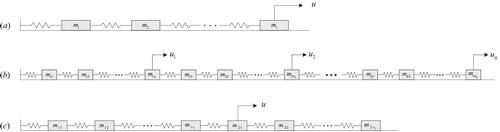
Multiple spring-mass systems

Consider the system (a) in Figure 1. By using the well-known Newton's Law, the set of basic equations of the system can be established as follows: (27) $\left\{\begin{array}{l}{m}_1{\ddot{x}}_1+c_1\left({\dot{x}}_1\right)+k_1{x}_1=k_2\left(x_2-x_1\right)\\ m_2{\ddot{x}}_2+c_2\left({\dot{x}}_2\right)+k_2\left(x_2-x_1\right)=k_3\left(x_3-x_2\right)\\ ⋮\\ m_{r-1}{\ddot{x}}_{r-1}+c_{r-1}\left({\dot{x}}_{r-1}\right)+k_{r-1}\left(x_{r-1}-x_{r-2}\right)\\ =k_r\left(x_r-x_{r-1}\right)\\ m_r{\ddot{x}}_r+c_r\left({\dot{x}}_r\right)+k_r\left(x_r-x_{r-1}\right)=u,\end{array}\right.$(27) where $m_i>0$ and $x_i$ are respectively the mass and the position of the ith moving object, $i=1,2,\dots ,r;$ $c_i\left({\dot{x}}_i\right),\text{ı}=1,2,\dots ,r,$ are a set of differentiable functions representing the friction forces, and $k_i>0,i=1,2,\dots ,r,$ are the spring coefficients.

Figure 1. Multiple spring-mass systems.

2.3.2. First- and high-order models

When a set of basic equations for a physical control system are obtained, we can further derive the desired type of models by rearranging the set of basic equations. There are basically two methods to fulfil this task, namely, the method of variable extension and the method of variable elimination. The former produces a first-order state-space model for a control system, while the latter gives a high-order model.

Due to the popularity of the state-space approaches, almost all models for physical control systems in the literature are finally converted into state-space forms, which are essentially a set of first-order differential equations. Since most of the original set of basic equations in (26(26) ${\alpha }_i\left(z^{\left(0\sim n_1\right)},u^{\left(0\sim n_2\right)},t\right)=0,i=1,2,\dots ,\kappa ,$(26) ) are of second-order, the state-space approach for modelling is essentially a method of variable extension. Without the extended variables, a set of high-order differential equations can be not at all equivalently turned into a set of first-order differential equations.

For over half a century of dominance, the state-space approaches have been completely accepted by the system and control community. State-space models have been taken universal. Control scientists and engineers have for long been so accustomed to establish a state-space model for any theoretical or practical system encountered, despite of the fact that, in most cases, the set of basic equations in (26(26) ${\alpha }_i\left(z^{\left(0\sim n_1\right)},u^{\left(0\sim n_2\right)},t\right)=0,i=1,2,\dots ,\kappa ,$(26) ) originally established by the physical laws are of second-order, and even may be already fully actuated.

It is not that state-space models are of the first priority, especially when dealing with the problem of control. It is not that high-order models have to be obtained from state-state models, while they should be directly obtained from the set of basic equations in the first place. Practically, most HOFA models should be obtained directly from the modelling process.

Example 2.6

Multiple spring-mass systems (Continued)

It is obvious that the set of basic equations in (27(27) $\left\{\begin{array}{l}{m}_1{\ddot{x}}_1+c_1\left({\dot{x}}_1\right)+k_1{x}_1=k_2\left(x_2-x_1\right)\\ m_2{\ddot{x}}_2+c_2\left({\dot{x}}_2\right)+k_2\left(x_2-x_1\right)=k_3\left(x_3-x_2\right)\\ ⋮\\ m_{r-1}{\ddot{x}}_{r-1}+c_{r-1}\left({\dot{x}}_{r-1}\right)+k_{r-1}\left(x_{r-1}-x_{r-2}\right)\\ =k_r\left(x_r-x_{r-1}\right)\\ m_r{\ddot{x}}_r+c_r\left({\dot{x}}_r\right)+k_r\left(x_r-x_{r-1}\right)=u,\end{array}\right.$(27) ) form a typical second-order strict-feedback system proposed in Duan (2021b). According to Theorem 3.2 in Duan (2021b), the above system (27(27) $\left\{\begin{array}{l}{m}_1{\ddot{x}}_1+c_1\left({\dot{x}}_1\right)+k_1{x}_1=k_2\left(x_2-x_1\right)\\ m_2{\ddot{x}}_2+c_2\left({\dot{x}}_2\right)+k_2\left(x_2-x_1\right)=k_3\left(x_3-x_2\right)\\ ⋮\\ m_{r-1}{\ddot{x}}_{r-1}+c_{r-1}\left({\dot{x}}_{r-1}\right)+k_{r-1}\left(x_{r-1}-x_{r-2}\right)\\ =k_r\left(x_r-x_{r-1}\right)\\ m_r{\ddot{x}}_r+c_r\left({\dot{x}}_r\right)+k_r\left(x_r-x_{r-1}\right)=u,\end{array}\right.$(27) ) can be equivalently converted into a HOFA system in the formof (28) $x_1^{\left(2r\right)}={\alpha }_a\left(x_1^{\left(0\sim 2r-1\right)}\right)+{\text{β}}_{a}u,$(28) where ${\alpha }_a\left(x_1^{(0\sim 2r-1)}\right)$ is a continuous function, and ${\text{β}}_a$ is a nonzero scalar. According to Theorem 3.2 in Duan (2021b), the other variables $x_i^{(0\sim 1)},\text{ı}=2,3,\dots ,r$, are determined by a differential homeomorphism between $x_1^{(0\sim 2r-1)}$ and $x_i^{(0\sim 1)},i=1,2,\dots ,r$.

The above (28(28) $x_1^{\left(2r\right)}={\alpha }_a\left(x_1^{\left(0\sim 2r-1\right)}\right)+{\text{β}}_{a}u,$(28) ) is obviously a HOFA model.

Based on the above fact, the spring-mass system (b) in Figure 1, with all the mass and the spring coefficient of each subsystem being greater than zero, can be equivalently converted into a HOFA model in the form of (29) $\left\{\begin{array}{l}{x}_{11}^{\left(2r_1\right)}={\alpha }_1\left(x_{11}^{\left(0\sim 2r_1-1\right)},x_{21}\right)+{\text{β}}_1{u}_1\\ x_{21}^{\left(2r_2\right)}={\alpha }_2\left(x_{11}^{\left(0\sim 2r_1-1\right)},x_{21}^{\left(0\sim 2r_2-1\right)},x_{31}\right)+{\text{β}}_2{u}_2\\ ⋮\\ x_{\eta 1}^{\left(2r_{\eta }\right)}={\alpha }_{\eta }\left(x_{k,1}^{\left(0\sim 2r_k-1\right)}{|}_{k=1\sim \eta }\right)+{\text{β}}_{\eta }{u}_{\eta },\end{array}\right.$(29) where ${\alpha }_i(\cdot )$ and ${\text{β}}_i$ are a nonlinear continuous function and a nonzero scalar, respectively, $i=1,2,\dots ,\eta$.

The above HOFA system (29(29) $\left\{\begin{array}{l}{x}_{11}^{\left(2r_1\right)}={\alpha }_1\left(x_{11}^{\left(0\sim 2r_1-1\right)},x_{21}\right)+{\text{β}}_1{u}_1\\ x_{21}^{\left(2r_2\right)}={\alpha }_2\left(x_{11}^{\left(0\sim 2r_1-1\right)},x_{21}^{\left(0\sim 2r_2-1\right)},x_{31}\right)+{\text{β}}_2{u}_2\\ ⋮\\ x_{\eta 1}^{\left(2r_{\eta }\right)}={\alpha }_{\eta }\left(x_{k,1}^{\left(0\sim 2r_k-1\right)}{|}_{k=1\sim \eta }\right)+{\text{β}}_{\eta }{u}_{\eta },\end{array}\right.$(29) ) is clearly in the form of (8(8) $\begin{array}{rl}\left[\begin{array}{c}{x}_1^{\left({\mu }_1\right)}\\ x_2^{\left({\mu }_2\right)}\\ ⋮\\ x_{\eta }^{\left({\mu }_{\eta }\right)}\end{array}\right]& =\left[\begin{array}{c}{f}_1\left(x_k^{\left(0\sim {\mu }_k-1\right)}{|}_{k=1\sim \eta },\zeta ,t\right)\\ f_2\left(x_k^{\left(0\sim {\mu }_k-1\right)}{|}_{k=1\sim \eta },\zeta ,t\right)\\ ⋮\\ f_{\eta }\left(x_k^{\left(0\sim {\mu }_k-1\right)}{|}_{k=1\sim \eta },\zeta ,t\right)\end{array}\right]\\ & +B\left(\cdot \right)u,\end{array}$(8) ).

3. Controllability

Controllability and stabilisability are two very important concepts in control systems theory. In this section we first investigate the controllability of general dynamical control systems.

3.1. A control feature of HOFA models

The following important fact about the control of the fully actuated system (8(8) $\begin{array}{rl}\left[\begin{array}{c}{x}_1^{\left({\mu }_1\right)}\\ x_2^{\left({\mu }_2\right)}\\ ⋮\\ x_{\eta }^{\left({\mu }_{\eta }\right)}\end{array}\right]& =\left[\begin{array}{c}{f}_1\left(x_k^{\left(0\sim {\mu }_k-1\right)}{|}_{k=1\sim \eta },\zeta ,t\right)\\ f_2\left(x_k^{\left(0\sim {\mu }_k-1\right)}{|}_{k=1\sim \eta },\zeta ,t\right)\\ ⋮\\ f_{\eta }\left(x_k^{\left(0\sim {\mu }_k-1\right)}{|}_{k=1\sim \eta },\zeta ,t\right)\end{array}\right]\\ & +B\left(\cdot \right)u,\end{array}$(8) ) or (10(10) $x_k^{\left({\mu }_k\right)}{|}_{k=1\sim \eta }=f\left(x_k^{\left(0\sim {\mu }_k-1\right)}{|}_{k=1\sim \eta },\zeta ,t\right)+B\left(\cdot \right)u.$(10) ) can be easily verified.

Proposition 3.1

Let $\mathrm{\Omega }\subset {\mathbb{R}}^{\varkappa }$ be a desired open set, and $\mathbb{F}\subset {\mathbb{R}}^{\varkappa }$ be the set of feasible points of the system (8(8) $\begin{array}{rl}\left[\begin{array}{c}{x}_1^{\left({\mu }_1\right)}\\ x_2^{\left({\mu }_2\right)}\\ ⋮\\ x_{\eta }^{\left({\mu }_{\eta }\right)}\end{array}\right]& =\left[\begin{array}{c}{f}_1\left(x_k^{\left(0\sim {\mu }_k-1\right)}{|}_{k=1\sim \eta },\zeta ,t\right)\\ f_2\left(x_k^{\left(0\sim {\mu }_k-1\right)}{|}_{k=1\sim \eta },\zeta ,t\right)\\ ⋮\\ f_{\eta }\left(x_k^{\left(0\sim {\mu }_k-1\right)}{|}_{k=1\sim \eta },\zeta ,t\right)\end{array}\right]\\ & +B\left(\cdot \right)u,\end{array}$(8) ), whose dimension is greater than 1. Further, let $[A_i{]}_{0\sim {\mu }_i-1}\in {\mathbb{R}}^{r_i\times {\mu }_i{r}_i},i=1,2,\dots ,\eta ,$ be a set of arbitrarily given matrices. Then the following controller (30) $\left\{\begin{array}{l}u=-B^{-1}\left(\cdot \right)\left(\left[\begin{array}{c}{\left[A_1\right]}_{0\sim {\mu }_1-1}{x}_1^{\left(0\sim {\mu }_1-1\right)}\\ {\left[A_2\right]}_{0\sim {\mu }_2-1}{x}_2^{\left(0\sim {\mu }_2-1\right)}\\ ⋮\\ {\left[A_{\eta }\right]}_{0\sim {\mu }_{\eta }-1}{x}_{\eta }^{\left(0\sim {\mu }_{\eta }-1\right)}\end{array}\right]+u^{\ast }\right)\\ u^{\ast }=f\left(x_k^{\left(0\sim {\mu }_k-1\right)}{|}_{k=1\sim \eta },\zeta ,t\right)-v,\end{array}\right.$(30) for system (8(8) $\begin{array}{rl}\left[\begin{array}{c}{x}_1^{\left({\mu }_1\right)}\\ x_2^{\left({\mu }_2\right)}\\ ⋮\\ x_{\eta }^{\left({\mu }_{\eta }\right)}\end{array}\right]& =\left[\begin{array}{c}{f}_1\left(x_k^{\left(0\sim {\mu }_k-1\right)}{|}_{k=1\sim \eta },\zeta ,t\right)\\ f_2\left(x_k^{\left(0\sim {\mu }_k-1\right)}{|}_{k=1\sim \eta },\zeta ,t\right)\\ ⋮\\ f_{\eta }\left(x_k^{\left(0\sim {\mu }_k-1\right)}{|}_{k=1\sim \eta },\zeta ,t\right)\end{array}\right]\\ & +B\left(\cdot \right)u,\end{array}$(8) ) produces the following constant linear closed-loop system (31) $x_k^{\left({\mu }_k\right)}+[A_k{]}_{0\sim {\mu }_k-1}{x}_k^{\left(0\sim {\mu }_k-1\right)}=v_k,k=1,2,\dots ,\eta ,$(31) with $v_k,$ $k=1,2,\dots ,\eta ,$ being defined by (32) $v=\left[\begin{array}{c}{v}_1\\ v_2\\ ⋮\\ v_{\eta }\end{array}\right],v_k\in {\mathbb{R}}^{r_k},$(32) provided that the states of the above closed-loop system (31(31) $x_k^{\left({\mu }_k\right)}+[A_k{]}_{0\sim {\mu }_k-1}{x}_k^{\left(0\sim {\mu }_k-1\right)}=v_k,k=1,2,\dots ,\eta ,$(31) ) satisfy (33) $x_k^{\left(0\sim {\mu }_k-1\right)}{|}_{k=1\sim \eta }\in \mathbb{F}.$(33)

Remark 3.1

For the more general fully actuated system (19(19) $x_k^{\left({\mu }_k\right)}{|}_{k=1\sim \eta }=f\left(x_k^{\left(0\sim {\mu }_k-1\right)}{|}_{k=1\sim \eta },\zeta ,t\right)+g\left(\cdot \right),$(19) ), a result similar to Proposition 3.1 still holds. In this case, the controller can be obtained using the differential homeomorphism property of the mapping $\tilde{u}=g(x_k^{(0\sim {\mu }_k-1)}{|}_{k=1\sim \eta },\zeta ,t,u),$ as (34) $\left\{\begin{array}{l}u=g^{-1}\left(x_k^{\left(0\sim {\mu }_k-1\right)}{|}_{k=1\sim \eta },\zeta ,t,\tilde{u}\right)\\ \tilde{u}=-\left(\left[\begin{array}{c}{\left[A_1\right]}_{0\sim {\mu }_1-1}{x}_1^{\left(0\sim {\mu }_1-1\right)}\\ {\left[A_2\right]}_{0\sim {\mu }_2-1}{x}_2^{\left(0\sim {\mu }_2-1\right)}\\ ⋮\\ {\left[A_{\eta }\right]}_{0\sim {\mu }_{\eta }-1}{x}_{\eta }^{\left(0\sim {\mu }_{\eta }-1\right)}\end{array}\right]+u^{\ast }\right)\\ u^{\ast }=f\left(x_k^{\left(0\sim {\mu }_k-1\right)}{|}_{k=1\sim \eta },\zeta ,t\right)-v,\end{array}\right.$(34) and the same closed-loop system as in (31(31) $x_k^{\left({\mu }_k\right)}+[A_k{]}_{0\sim {\mu }_k-1}{x}_k^{\left(0\sim {\mu }_k-1\right)}=v_k,k=1,2,\dots ,\eta ,$(31) ) is achieved.

Since the closed-loop system (31(31) $x_k^{\left({\mu }_k\right)}+[A_k{]}_{0\sim {\mu }_k-1}{x}_k^{\left(0\sim {\mu }_k-1\right)}=v_k,k=1,2,\dots ,\eta ,$(31) ) is linear, for convenience we call the controller in the form of (30(30) $\left\{\begin{array}{l}u=-B^{-1}\left(\cdot \right)\left(\left[\begin{array}{c}{\left[A_1\right]}_{0\sim {\mu }_1-1}{x}_1^{\left(0\sim {\mu }_1-1\right)}\\ {\left[A_2\right]}_{0\sim {\mu }_2-1}{x}_2^{\left(0\sim {\mu }_2-1\right)}\\ ⋮\\ {\left[A_{\eta }\right]}_{0\sim {\mu }_{\eta }-1}{x}_{\eta }^{\left(0\sim {\mu }_{\eta }-1\right)}\end{array}\right]+u^{\ast }\right)\\ u^{\ast }=f\left(x_k^{\left(0\sim {\mu }_k-1\right)}{|}_{k=1\sim \eta },\zeta ,t\right)-v,\end{array}\right.$(30) ), or (34(34) $\left\{\begin{array}{l}u=g^{-1}\left(x_k^{\left(0\sim {\mu }_k-1\right)}{|}_{k=1\sim \eta },\zeta ,t,\tilde{u}\right)\\ \tilde{u}=-\left(\left[\begin{array}{c}{\left[A_1\right]}_{0\sim {\mu }_1-1}{x}_1^{\left(0\sim {\mu }_1-1\right)}\\ {\left[A_2\right]}_{0\sim {\mu }_2-1}{x}_2^{\left(0\sim {\mu }_2-1\right)}\\ ⋮\\ {\left[A_{\eta }\right]}_{0\sim {\mu }_{\eta }-1}{x}_{\eta }^{\left(0\sim {\mu }_{\eta }-1\right)}\end{array}\right]+u^{\ast }\right)\\ u^{\ast }=f\left(x_k^{\left(0\sim {\mu }_k-1\right)}{|}_{k=1\sim \eta },\zeta ,t\right)-v,\end{array}\right.$(34) ), a linearising controller for the HOFA system (8(8) $\begin{array}{rl}\left[\begin{array}{c}{x}_1^{\left({\mu }_1\right)}\\ x_2^{\left({\mu }_2\right)}\\ ⋮\\ x_{\eta }^{\left({\mu }_{\eta }\right)}\end{array}\right]& =\left[\begin{array}{c}{f}_1\left(x_k^{\left(0\sim {\mu }_k-1\right)}{|}_{k=1\sim \eta },\zeta ,t\right)\\ f_2\left(x_k^{\left(0\sim {\mu }_k-1\right)}{|}_{k=1\sim \eta },\zeta ,t\right)\\ ⋮\\ f_{\eta }\left(x_k^{\left(0\sim {\mu }_k-1\right)}{|}_{k=1\sim \eta },\zeta ,t\right)\end{array}\right]\\ & +B\left(\cdot \right)u,\end{array}$(8) ). When expanded, each subsystem in the above linear closed-loop system (31(31) $x_k^{\left({\mu }_k\right)}+[A_k{]}_{0\sim {\mu }_k-1}{x}_k^{\left(0\sim {\mu }_k-1\right)}=v_k,k=1,2,\dots ,\eta ,$(31) ) can be written as $\begin{array}{rl}& x_k^{\left({\mu }_k\right)}+[A_k{]}_{{\mu }_k-1}{x}^{\left({\mu }_k-1\right)}\\ & +\cdots +[A_k{]}_1\dot{x}+[A_k{]}_{0}x=v_k,\end{array}$whose eigen-polynomial matrix obviously is $\begin{array}{rl}{P}_k\left(s\right)& =I_{r_k}{s}^{{\mu }_k}+[A_k{]}_{{\mu }_k-1}{s}^{{\mu }_k-1}\\ & +\cdots +[A_k{]}_{1}s+[A_k{]}_0.\end{array}$Due to the arbitrariness of the series of matrices $[A_k{]}_i,\text{ı}=0,1,\dots ,{\mu }_k-1$, $k=1,2,\dots ,\eta ,$ the eigen-polynomial matrices of each subsystem in the linear closed-loop system (31(31) $x_k^{\left({\mu }_k\right)}+[A_k{]}_{0\sim {\mu }_k-1}{x}_k^{\left(0\sim {\mu }_k-1\right)}=v_k,k=1,2,\dots ,\eta ,$(31) ) can be arbitrarily assigned. Therefore, a linear closed-loop system with desired performance can be obtained by properly selecting these matrices. Particularly, the closed-loop eigenvalues can be arbitrarily assigned by properly selecting these matrices. Such a property of HOFA systems totally reveals the meaning of controllability of control systems.

3.2. Definition of controllability

Introduce the following general nonlinear system (35) $F\left(z^{\left(0\sim n\right)},u,t\right)=0,$(35) where $F(\cdot )$ is a vector function of appropriate dimension, and z and u are respectively the state and input vectors of appropriate dimensions, n is an integer. Regarding the controllability of the system (35(35) $F\left(z^{\left(0\sim n\right)},u,t\right)=0,$(35) ), we propose the following definition.

Definition 3.2

The dynamical system (35(35) $F\left(z^{\left(0\sim n\right)},u,t\right)=0,$(35) ) is called

• completely controllable if it can be equivalently converted into a globally fully actuated system in the form of (8(8) $\begin{array}{rl}\left[\begin{array}{c}{x}_1^{\left({\mu }_1\right)}\\ x_2^{\left({\mu }_2\right)}\\ ⋮\\ x_{\eta }^{\left({\mu }_{\eta }\right)}\end{array}\right]& =\left[\begin{array}{c}{f}_1\left(x_k^{\left(0\sim {\mu }_k-1\right)}{|}_{k=1\sim \eta },\zeta ,t\right)\\ f_2\left(x_k^{\left(0\sim {\mu }_k-1\right)}{|}_{k=1\sim \eta },\zeta ,t\right)\\ ⋮\\ f_{\eta }\left(x_k^{\left(0\sim {\mu }_k-1\right)}{|}_{k=1\sim \eta },\zeta ,t\right)\end{array}\right]\\ & +B\left(\cdot \right)u,\end{array}$(8) ) or (19(19) $x_k^{\left({\mu }_k\right)}{|}_{k=1\sim \eta }=f\left(x_k^{\left(0\sim {\mu }_k-1\right)}{|}_{k=1\sim \eta },\zeta ,t\right)+g\left(\cdot \right),$(19) );

• almost completely controllable if it can be equivalently converted into an almost fully actuated system in the form of (8(8) $\begin{array}{rl}\left[\begin{array}{c}{x}_1^{\left({\mu }_1\right)}\\ x_2^{\left({\mu }_2\right)}\\ ⋮\\ x_{\eta }^{\left({\mu }_{\eta }\right)}\end{array}\right]& =\left[\begin{array}{c}{f}_1\left(x_k^{\left(0\sim {\mu }_k-1\right)}{|}_{k=1\sim \eta },\zeta ,t\right)\\ f_2\left(x_k^{\left(0\sim {\mu }_k-1\right)}{|}_{k=1\sim \eta },\zeta ,t\right)\\ ⋮\\ f_{\eta }\left(x_k^{\left(0\sim {\mu }_k-1\right)}{|}_{k=1\sim \eta },\zeta ,t\right)\end{array}\right]\\ & +B\left(\cdot \right)u,\end{array}$(8) ) or (19(19) $x_k^{\left({\mu }_k\right)}{|}_{k=1\sim \eta }=f\left(x_k^{\left(0\sim {\mu }_k-1\right)}{|}_{k=1\sim \eta },\zeta ,t\right)+g\left(\cdot \right),$(19) );

• basically completely controllable if it can be equivalently converted into a basically fully actuated system in the form of (8(8) $\begin{array}{rl}\left[\begin{array}{c}{x}_1^{\left({\mu }_1\right)}\\ x_2^{\left({\mu }_2\right)}\\ ⋮\\ x_{\eta }^{\left({\mu }_{\eta }\right)}\end{array}\right]& =\left[\begin{array}{c}{f}_1\left(x_k^{\left(0\sim {\mu }_k-1\right)}{|}_{k=1\sim \eta },\zeta ,t\right)\\ f_2\left(x_k^{\left(0\sim {\mu }_k-1\right)}{|}_{k=1\sim \eta },\zeta ,t\right)\\ ⋮\\ f_{\eta }\left(x_k^{\left(0\sim {\mu }_k-1\right)}{|}_{k=1\sim \eta },\zeta ,t\right)\end{array}\right]\\ & +B\left(\cdot \right)u,\end{array}$(8) ) or (19(19) $x_k^{\left({\mu }_k\right)}{|}_{k=1\sim \eta }=f\left(x_k^{\left(0\sim {\mu }_k-1\right)}{|}_{k=1\sim \eta },\zeta ,t\right)+g\left(\cdot \right),$(19) ); and

• controllable on a set $\mathrm{\Omega }\subset {\mathbb{R}}^{\varkappa }$, $\varkappa =\sum _{i=1}^{\eta }{r}_k{\mu }_k,$ if it can be equivalently converted into a system in the form of (8(8) $\begin{array}{rl}\left[\begin{array}{c}{x}_1^{\left({\mu }_1\right)}\\ x_2^{\left({\mu }_2\right)}\\ ⋮\\ x_{\eta }^{\left({\mu }_{\eta }\right)}\end{array}\right]& =\left[\begin{array}{c}{f}_1\left(x_k^{\left(0\sim {\mu }_k-1\right)}{|}_{k=1\sim \eta },\zeta ,t\right)\\ f_2\left(x_k^{\left(0\sim {\mu }_k-1\right)}{|}_{k=1\sim \eta },\zeta ,t\right)\\ ⋮\\ f_{\eta }\left(x_k^{\left(0\sim {\mu }_k-1\right)}{|}_{k=1\sim \eta },\zeta ,t\right)\end{array}\right]\\ & +B\left(\cdot \right)u,\end{array}$(8) ) or (19(19) $x_k^{\left({\mu }_k\right)}{|}_{k=1\sim \eta }=f\left(x_k^{\left(0\sim {\mu }_k-1\right)}{|}_{k=1\sim \eta },\zeta ,t\right)+g\left(\cdot \right),$(19) ), which is fully actuated on Ω.

Furthermore, the dynamical system (35(35) $F\left(z^{\left(0\sim n\right)},u,t\right)=0,$(35) ) is generally called controllable if it is controllable at least on a set with dimension greater than one.

The above definition obviously contains Definition 3 in Duan (2020b) as a special case. With this definition, it is obvious that

• all dynamical control systems, not only those in state-space representations, possess the concepts of controllability;

• the problem of controllability analysis and the problem of control are now highly consistent in the sense that, once the controllability of a system is verified by obtaining the HOFA model of the system, the design problem is then easily solved in view of Proposition 3.1.

Now let us consider again modelling a physical system ${\mathrm{\Sigma }}_{\mathrm{p}\mathrm{h}\mathrm{y}\mathrm{s}\mathrm{i}\mathrm{c}\mathrm{a}\mathrm{l}}$ by mechanism. To be more strict, let us impose the following assumption:

Assumption A1

The considered physical system ${\mathrm{\Sigma }}_{\mathrm{p}\mathrm{h}\mathrm{y}\mathrm{s}\mathrm{i}\mathrm{c}\mathrm{a}\mathrm{l}},$ with basic equations in (26(26) ${\alpha }_i\left(z^{\left(0\sim n_1\right)},u^{\left(0\sim n_2\right)},t\right)=0,i=1,2,\dots ,\kappa ,$(26) ), has r number of independent and functioning control variables.

As mentioned above, once we obtain the basic equations in (26(26) ${\alpha }_i\left(z^{\left(0\sim n_1\right)},u^{\left(0\sim n_2\right)},t\right)=0,i=1,2,\dots ,\kappa ,$(26) ) by mechanism for a physical system ${\mathrm{\Sigma }}_{\mathrm{p}\mathrm{h}\mathrm{y}\mathrm{s}\mathrm{i}\mathrm{c}\mathrm{a}\mathrm{l}}$, on one hand one can obtain a state-space model by the method of variable extension, while on the other hand one can get a high-order model for the system by the method of variable elimination. As a result, the state-space model obtained by the method of variable extension contains the maximum number of independent scalar equations, while the number of scalar equations in a high-order model obtained by the method of variable elimination gets fewer as the order of the model goes higher.

Now the questions is, how few can the scalar equations in a finally obtained high-order model be? There must be a smallest number of scalar equations in such a finally obtained high-order model. On one side, the number of scalar equations is generally not less than r since otherwise the system would have fewer than r control variables, and this would contradict with Assumption A1. On the other side, the number of scalar equations is getting close to r as the process of variable elimination goes. For a system which is ‘completely controllable’, in the sense that the whole set of control variables fully determine the dynamics of the system, the smallest number of scalar equations in the finally obtained high-order model becomes r, in this case a HOFA model for the system ${\mathrm{\Sigma }}_{\mathrm{p}\mathrm{h}\mathrm{y}\mathrm{s}\mathrm{i}\mathrm{c}\mathrm{a}\mathrm{l}}$ is derived.

To summarise, we immediately have the following fact.

Proposition 3.3

Let (26(26) ${\alpha }_i\left(z^{\left(0\sim n_1\right)},u^{\left(0\sim n_2\right)},t\right)=0,i=1,2,\dots ,\kappa ,$(26) ) be the set of basic equations of the original physical system ${\mathrm{\Sigma }}_{\mathrm{p}\mathrm{h}\mathrm{y}\mathrm{s}\mathrm{i}\mathrm{c}\mathrm{a}\mathrm{l}}$ satisfying Assumption A1. Further, assume that the set of control variables of system ${\mathrm{\Sigma }}_{\mathrm{p}\mathrm{h}\mathrm{y}\mathrm{s}\mathrm{i}\mathrm{c}\mathrm{a}\mathrm{l}}$ fully determine the dynamics of the system. Then the set of basic equations in (26(26) ${\alpha }_i\left(z^{\left(0\sim n_1\right)},u^{\left(0\sim n_2\right)},t\right)=0,i=1,2,\dots ,\kappa ,$(26) ) can be further converted into a HOFA model in the form of (8(8) $\begin{array}{rl}\left[\begin{array}{c}{x}_1^{\left({\mu }_1\right)}\\ x_2^{\left({\mu }_2\right)}\\ ⋮\\ x_{\eta }^{\left({\mu }_{\eta }\right)}\end{array}\right]& =\left[\begin{array}{c}{f}_1\left(x_k^{\left(0\sim {\mu }_k-1\right)}{|}_{k=1\sim \eta },\zeta ,t\right)\\ f_2\left(x_k^{\left(0\sim {\mu }_k-1\right)}{|}_{k=1\sim \eta },\zeta ,t\right)\\ ⋮\\ f_{\eta }\left(x_k^{\left(0\sim {\mu }_k-1\right)}{|}_{k=1\sim \eta },\zeta ,t\right)\end{array}\right]\\ & +B\left(\cdot \right)u,\end{array}$(8) ) or (19(19) $x_k^{\left({\mu }_k\right)}{|}_{k=1\sim \eta }=f\left(x_k^{\left(0\sim {\mu }_k-1\right)}{|}_{k=1\sim \eta },\zeta ,t\right)+g\left(\cdot \right),$(19) ) by applying the method of variable elimination.

The fact mentioned in the above Proposition 3.3 has been demonstrated by many examples (see those in Duan, 2020d, 2020e, 2021a, 2021b, 2021c, 2021d). While in the case where the considered system ${\mathrm{\Sigma }}_{\mathrm{p}\mathrm{h}\mathrm{y}\mathrm{s}\mathrm{i}\mathrm{c}\mathrm{a}\mathrm{l}}$ or (26(26) ${\alpha }_i\left(z^{\left(0\sim n_1\right)},u^{\left(0\sim n_2\right)},t\right)=0,i=1,2,\dots ,\kappa ,$(26) ) is not controllable, its model appears to be more complicated.

According to the above definition, the system presented in Example 2.4 is clearly an almost completely controllable one. Following the above Proposition 3.1, a controller can be properly designed to produce a constant linear system. Therefore, with a choice of proper set of initial values, the amplitude of the pitch angle ϑ can be kept well within $(-\pi /2,\pi /2)$. Hence the designed control system works (see Duan, 2014 for detail). To further demonstrate the approach, let us present another simple example.

Example 3.4

Consider the following system (36) $\left\{\begin{array}{l}\ddot{x}=\mathrm{t}\mathrm{g}\theta ,\left|\theta \right|<\frac{\pi }{2}\\ \ddot{\theta }=u,\end{array}\right.$(36) where u is a scalar input. Using the first equation in (36(36) $\left\{\begin{array}{l}\ddot{x}=\mathrm{t}\mathrm{g}\theta ,\left|\theta \right|<\frac{\pi }{2}\\ \ddot{\theta }=u,\end{array}\right.$(36) ), we obtain (37) $\theta =\mathrm{a}\mathrm{r}\mathrm{c}\mathrm{t}\mathrm{g}\left(\ddot{x}\right),$(37) from which we can easily derive (38) $\dot{\theta }=\frac{1}{1+{\ddot{x}}^2}\stackrel{⃛}{x},$(38) and further (39) $\begin{array}{rl}\ddot{\theta }& ={\left(\frac{1}{1+{\ddot{x}}^2}\right)}^{\mathrm{\prime }}\stackrel{⃛}{x}+\frac{1}{1+{\ddot{x}}^2}{x}^{\left(4\right)}\\ & =\frac{1}{1+{\ddot{x}}^2}{x}^{\left(4\right)}-\frac{2}{{\left(1+{\ddot{x}}^2\right)}^2}\ddot{x}{\stackrel{⃛}{x}}^2.\end{array}$(39) Substituting the above equation into the second equation in (36(36) $\left\{\begin{array}{l}\ddot{x}=\mathrm{t}\mathrm{g}\theta ,\left|\theta \right|<\frac{\pi }{2}\\ \ddot{\theta }=u,\end{array}\right.$(36) ), yields (40) $x^{\left(4\right)}-\frac{2}{1+{\ddot{x}}^2}\ddot{x}{\stackrel{⃛}{x}}^2=\left(1+{\ddot{x}}^2\right)u.$(40) This is the HOFA model of system (36(36) $\left\{\begin{array}{l}\ddot{x}=\mathrm{t}\mathrm{g}\theta ,\left|\theta \right|<\frac{\pi }{2}\\ \ddot{\theta }=u,\end{array}\right.$(36) ). Note that $1+{\ddot{x}}^2\ne 0$, the above system (40(40) $x^{\left(4\right)}-\frac{2}{1+{\ddot{x}}^2}\ddot{x}{\stackrel{⃛}{x}}^2=\left(1+{\ddot{x}}^2\right)u.$(40) ) is globally fully actuated, hence the system (36(36) $\left\{\begin{array}{l}\ddot{x}=\mathrm{t}\mathrm{g}\theta ,\left|\theta \right|<\frac{\pi }{2}\\ \ddot{\theta }=u,\end{array}\right.$(36) ) is completely controllable.

For control of the above HOFA system (40(40) $x^{\left(4\right)}-\frac{2}{1+{\ddot{x}}^2}\ddot{x}{\stackrel{⃛}{x}}^2=\left(1+{\ddot{x}}^2\right)u.$(40) ), we can follow the standard procedure, and choose (41) $u=-\frac{1}{1+{\ddot{x}}^2}\left(\frac{2}{1+{\ddot{x}}^2}\ddot{x}{\stackrel{⃛}{x}}^2+\sum _{i=0}^3{a}_i{x}^{\left(i\right)}-v\right),$(41) where $a_i,i=0,1,2,3,$ are some real scalars, and v is an external scalar input. Then the closed-loop system is (42) $x^{\left(4\right)}+\sum _{i=0}^3{a}_i{x}^{\left(i\right)}=v,$(42) where $a_i,i=0,1,2,3,$ can be properly chosen such that the above system possesses a set of desired poles. Therefore, all $x^{\left(i\right)},\text{ı}=0,1,2,3,$ are determined by the above system, and $\theta ,\dot{\theta }$ and $\ddot{\theta }$ are then determined by (37(37) $\theta =\mathrm{a}\mathrm{r}\mathrm{c}\mathrm{t}\mathrm{g}\left(\ddot{x}\right),$(37) )–(39(39) $\begin{array}{rl}\ddot{\theta }& ={\left(\frac{1}{1+{\ddot{x}}^2}\right)}^{\mathrm{\prime }}\stackrel{⃛}{x}+\frac{1}{1+{\ddot{x}}^2}{x}^{\left(4\right)}\\ & =\frac{1}{1+{\ddot{x}}^2}{x}^{\left(4\right)}-\frac{2}{{\left(1+{\ddot{x}}^2\right)}^2}\ddot{x}{\stackrel{⃛}{x}}^2.\end{array}$(39) ), with the restriction of $\left|\theta \right|<\frac{\pi }{2}$.

To end this section, let us re-examine the multiple spring-mass systems treated in Examples 2.5 and 2.6.

Example 3.5

Multiple spring-mass systems (Continued)

By our definition of controllability, it follows from Examples 2.5 and 2.6 that the systems (a) and (b) in Figure 1 are both completely controllable when the friction forces and spring forces on each moving object are different from zero.

Now, let us further consider the system (c) in Figure 1. Again, the basic equations can be easily established by using Newton's Law as (43) $\left\{\begin{array}{l}{m}_{11}{\ddot{x}}_{11}+c_{11}\left({\dot{x}}_{11}\right)+k_{11}{x}_{11}=k_{12}\left(x_{12}-x_{11}\right)\\ m_{12}{\ddot{x}}_{12}+c_{12}\left({\dot{x}}_{12}\right)+k_{12}\left(x_{12}-x_{11}\right)\\ =k_{13}\left(x_{13}-x_{12}\right)\\ ⋮\\ m_{1r_1}{\ddot{x}}_{1r_1}+c_{1r_1}\left({\dot{x}}_{1r_1}\right)+k_{1r_1}\left(x_{1r_1}-x_{1,r_1-1}\right)\\ =k_{21}\left(x_{21}-x_{1r_1}\right),\end{array}\right.$(43) and (44) $\left\{\begin{array}{l}{m}_{21}{\ddot{x}}_{21}+c_{21}\left({\dot{x}}_{21}\right)+k_{21}\left(x_{21}-x_{1r_1}\right)\\ =k_{22}\left(x_{22}-x_{21}\right)+u\\ m_{22}{\ddot{x}}_{22}+c_{22}\left({\dot{x}}_{22}\right)+k_{22}\left(x_{22}-x_{21}\right)\\ =k_{23}\left(x_{23}-x_{22}\right)\\ ⋮\\ m_{2r_2}{\ddot{x}}_{2r_2}+c_{2r_2}\left({\dot{x}}_{2r_2}\right)+k_{2r_2}\left(x_{2r_2}-x_{2,r_2-1}\right)=0\end{array}\right.$(44) where $m_{ij}>0$ and $x_{ij}$ are the mass and the position of the $(i,j)$th object, $j=1,2,\dots ,r_i,$ $i=1,2;$ $c_{ij}\left({\dot{x}}_{ij}\right)$, $j=1,2,\dots ,r_i,$ $i=1,2,$ are a set of differential functions representing the friction forces, and $k_{ij}>0,$ $j=1,2,\dots ,r_i$, i = 1, 2, are the spring coefficients.

Rewriting the equations in (44(44) $\left\{\begin{array}{l}{m}_{21}{\ddot{x}}_{21}+c_{21}\left({\dot{x}}_{21}\right)+k_{21}\left(x_{21}-x_{1r_1}\right)\\ =k_{22}\left(x_{22}-x_{21}\right)+u\\ m_{22}{\ddot{x}}_{22}+c_{22}\left({\dot{x}}_{22}\right)+k_{22}\left(x_{22}-x_{21}\right)\\ =k_{23}\left(x_{23}-x_{22}\right)\\ ⋮\\ m_{2r_2}{\ddot{x}}_{2r_2}+c_{2r_2}\left({\dot{x}}_{2r_2}\right)+k_{2r_2}\left(x_{2r_2}-x_{2,r_2-1}\right)=0\end{array}\right.$(44) ) by reversing the orders of the equations, we obtain (45) $\left\{\begin{array}{l}{m}_{2r_2}{\ddot{x}}_{2r_2}+c_{2r_2}\left({\dot{x}}_{2r_2}\right)+k_{2r_2}{x}_{2r_2}=k_{2r_2}{x}_{2,r_2-1}\\ m_{2,r_2-1}{\ddot{x}}_{2,r_2-1}+c_{2,r_2-1}\left({\dot{x}}_{2,r_2-1}\right)\\ +k_{2,r_2-1}\left(x_{2,r_2-1}-x_{2,r_2-2}\right)\\ =k_{2r_2}\left(x_{2r_2}-x_{2,r_2-1}\right)\\ ⋮\\ m_{21}{\ddot{x}}_{21}+c_{21}\left({\dot{x}}_{21}\right)+k_{21}\left(x_{21}-x_{1r_1}\right)\\ =k_{22}\left(x_{22}-x_{21}\right)+u,\end{array}\right.$(45) which also forms a typical second-order strict-feedback system proposed in Duan (2021b). Again, according to Theorem 3.2 in Duan (2021b), the above system (45(45) $\left\{\begin{array}{l}{m}_{2r_2}{\ddot{x}}_{2r_2}+c_{2r_2}\left({\dot{x}}_{2r_2}\right)+k_{2r_2}{x}_{2r_2}=k_{2r_2}{x}_{2,r_2-1}\\ m_{2,r_2-1}{\ddot{x}}_{2,r_2-1}+c_{2,r_2-1}\left({\dot{x}}_{2,r_2-1}\right)\\ +k_{2,r_2-1}\left(x_{2,r_2-1}-x_{2,r_2-2}\right)\\ =k_{2r_2}\left(x_{2r_2}-x_{2,r_2-1}\right)\\ ⋮\\ m_{21}{\ddot{x}}_{21}+c_{21}\left({\dot{x}}_{21}\right)+k_{21}\left(x_{21}-x_{1r_1}\right)\\ =k_{22}\left(x_{22}-x_{21}\right)+u,\end{array}\right.$(45) ) can be equivalently converted into a HOFA system in the form of (46) $x_{2,r_2}^{\left(2r_2\right)}={\alpha }_0\left(x_{2,r_2}^{\left(0\sim 2r_2-1\right)}\right)+{\text{β}}_0\left(u+k_{21}{x}_{1,r_1}\right),$(46) where ${\alpha }_0\left(x_{2,r_2}^{(0\sim 2r_2-1)}\right)$ is a continuous function, and ${\text{β}}_0$ is a nonzero scalar. Now, combining (43(43) $\left\{\begin{array}{l}{m}_{11}{\ddot{x}}_{11}+c_{11}\left({\dot{x}}_{11}\right)+k_{11}{x}_{11}=k_{12}\left(x_{12}-x_{11}\right)\\ m_{12}{\ddot{x}}_{12}+c_{12}\left({\dot{x}}_{12}\right)+k_{12}\left(x_{12}-x_{11}\right)\\ =k_{13}\left(x_{13}-x_{12}\right)\\ ⋮\\ m_{1r_1}{\ddot{x}}_{1r_1}+c_{1r_1}\left({\dot{x}}_{1r_1}\right)+k_{1r_1}\left(x_{1r_1}-x_{1,r_1-1}\right)\\ =k_{21}\left(x_{21}-x_{1r_1}\right),\end{array}\right.$(43) ) with the above (46(46) $x_{2,r_2}^{\left(2r_2\right)}={\alpha }_0\left(x_{2,r_2}^{\left(0\sim 2r_2-1\right)}\right)+{\text{β}}_0\left(u+k_{21}{x}_{1,r_1}\right),$(46) ), gives the following set of equations describing the system (c) in Figure 1: (47) $\left\{\begin{array}{l}{m}_{11}{\ddot{x}}_{11}+c_{11}\left({\dot{x}}_{11}\right)+k_{11}{x}_{11}=k_{12}\left(x_{12}-x_{11}\right)\\ m_{12}{\ddot{x}}_{12}+c_{12}\left({\dot{x}}_{12}\right)+k_{12}\left(x_{12}-x_{11}\right)\\ =k_{13}\left(x_{13}-x_{12}\right)\\ ⋮\\ m_{1r_1}{\ddot{x}}_{1r_1}+c_{1r_1}\left({\dot{x}}_{1r_1}\right)+k_{1r_1}\left(x_{1r_1}-x_{1,r_1-1}\right)\\ =k_{21}\left(x_{21}-x_{1r_1}\right)\\ x_{2,r_2}^{\left(2r_2\right)}={\alpha }_0\left(x_{2,r_2}^{\left(0\sim 2r_2-1\right)}\right)+{\text{β}}_0\left(u+k_{21}{x}_{1,r_1}\right).\end{array}\right.$(47) It is easily recognised that the above system (47(47) $\left\{\begin{array}{l}{m}_{11}{\ddot{x}}_{11}+c_{11}\left({\dot{x}}_{11}\right)+k_{11}{x}_{11}=k_{12}\left(x_{12}-x_{11}\right)\\ m_{12}{\ddot{x}}_{12}+c_{12}\left({\dot{x}}_{12}\right)+k_{12}\left(x_{12}-x_{11}\right)\\ =k_{13}\left(x_{13}-x_{12}\right)\\ ⋮\\ m_{1r_1}{\ddot{x}}_{1r_1}+c_{1r_1}\left({\dot{x}}_{1r_1}\right)+k_{1r_1}\left(x_{1r_1}-x_{1,r_1-1}\right)\\ =k_{21}\left(x_{21}-x_{1r_1}\right)\\ x_{2,r_2}^{\left(2r_2\right)}={\alpha }_0\left(x_{2,r_2}^{\left(0\sim 2r_2-1\right)}\right)+{\text{β}}_0\left(u+k_{21}{x}_{1,r_1}\right).\end{array}\right.$(47) ) is a mixed-order strict-feedback system, proposed in Duan (2021b). According to Theorem 3.3 in Duan (2021b), the above system (47(47) $\left\{\begin{array}{l}{m}_{11}{\ddot{x}}_{11}+c_{11}\left({\dot{x}}_{11}\right)+k_{11}{x}_{11}=k_{12}\left(x_{12}-x_{11}\right)\\ m_{12}{\ddot{x}}_{12}+c_{12}\left({\dot{x}}_{12}\right)+k_{12}\left(x_{12}-x_{11}\right)\\ =k_{13}\left(x_{13}-x_{12}\right)\\ ⋮\\ m_{1r_1}{\ddot{x}}_{1r_1}+c_{1r_1}\left({\dot{x}}_{1r_1}\right)+k_{1r_1}\left(x_{1r_1}-x_{1,r_1-1}\right)\\ =k_{21}\left(x_{21}-x_{1r_1}\right)\\ x_{2,r_2}^{\left(2r_2\right)}={\alpha }_0\left(x_{2,r_2}^{\left(0\sim 2r_2-1\right)}\right)+{\text{β}}_0\left(u+k_{21}{x}_{1,r_1}\right).\end{array}\right.$(47) ) can be equivalently converted into a HOFA system in the form of $x_{11}^{\left(2\left(r_1+r_2\right)\right)}={\alpha }_b\left(x_{11}^{\left(0\sim 2\left(r_1+r_2\right)-1\right)}\right)+{\text{β}}_{b}u,$where ${\alpha }_b\left(x_{11}^{(0\sim 2(r_1+r_2)-1)}\right)$ is a continuous function, and ${\text{β}}_b$ is a nonzero scalar.

Therefore, the system (c) in Figure 1 is also completely controllable.

Based on the above conclusions, we can further deduce the following conclusion: the system (b) in Figure 1, with the mass and the spring coefficient of each subsystem being greater than zero, is completely controllable if and only if at least one of the forces $u_i,\text{ı}=1,2,\dots ,\eta ,$ is not constantly zero.

4. Stabilisability

Like controllability, stabilisability is also one of the most important concepts in control systems theory. This section further looks into the problem of stabilisability.

4.1. Type I systems

As addressed in Section 2.3, corresponding to the method of variable extension with which a state-space model can be established, there is also the method of variable elimination, with which a high-order differential equation model can be established.

In the case that the considered system ${\mathrm{\Sigma }}_{\mathrm{p}\mathrm{h}\mathrm{y}\mathrm{s}\mathrm{i}\mathrm{c}\mathrm{a}\mathrm{l}}$ or (26(26) ${\alpha }_i\left(z^{\left(0\sim n_1\right)},u^{\left(0\sim n_2\right)},t\right)=0,i=1,2,\dots ,\kappa ,$(26) ) is not controllable, besides a HOFA subsystem, the model of the system also contains an extra autonomous subsystem. More specifically, let us give the following proposition.

Proposition 4.1

Consider the system represented by (26(26) ${\alpha }_i\left(z^{\left(0\sim n_1\right)},u^{\left(0\sim n_2\right)},t\right)=0,i=1,2,\dots ,\kappa ,$(26) ), or the original physical system ${\mathrm{\Sigma }}_{\mathrm{p}\mathrm{h}\mathrm{y}\mathrm{s}\mathrm{i}\mathrm{c}\mathrm{a}\mathrm{l}},$ satisfying Assumption A1. If the system is not controllable, then it may possess a high-order system model consisting of (48) $\begin{array}{rl}{x}_k^{\left({\mu }_k\right)}{|}_{k=1\sim \eta }& =f\left(x_k^{\left(0\sim {\mu }_k-1\right)}{|}_{k=1\sim \eta },\right.\\ & \left.y_k^{\left(0\sim {\gamma }_k-1\right)}{|}_{k=1\sim \xi },\zeta ,t\right)\\ & +B\left(x_k^{\left(0\sim {\mu }_k-1\right)}{|}_{k=1\sim \eta },\right.\\ & \left.y_k^{\left(0\sim {\gamma }_k-1\right)}{|}_{k=1\sim \xi },\zeta ,t\right)u,\end{array}$(48) and (49) $y_k^{\left({\gamma }_k\right)}{|}_{k=1\sim \xi }=g\left(y_k^{\left(0\sim {\gamma }_k-1\right)}{|}_{k=1\sim \xi },\zeta ,t\right),$(49) where $\zeta \in {\mathbb{R}}^p$ is an external vector, ${\gamma }_k,=1,2,\dots ,\xi ,$ are a set of integers, $y_k,k=1,2,\dots ,\xi ,$ are a set of vectors of proper dimensions, $f(\cdot )$ and $g(\cdot )$ are two nonlinear vector functions, while the variables in (48(48) $\begin{array}{rl}{x}_k^{\left({\mu }_k\right)}{|}_{k=1\sim \eta }& =f\left(x_k^{\left(0\sim {\mu }_k-1\right)}{|}_{k=1\sim \eta },\right.\\ & \left.y_k^{\left(0\sim {\gamma }_k-1\right)}{|}_{k=1\sim \xi },\zeta ,t\right)\\ & +B\left(x_k^{\left(0\sim {\mu }_k-1\right)}{|}_{k=1\sim \eta },\right.\\ & \left.y_k^{\left(0\sim {\gamma }_k-1\right)}{|}_{k=1\sim \xi },\zeta ,t\right)u,\end{array}$(48) ) are as stated before. It is required that $y_k^{(0\sim {\gamma }_k-1)}{|}_{k=1\sim \xi }$ and $x_k^{(0\sim {\mu }_k-1)}{|}_{k=1\sim \eta }$ are independent from each other, and the following full-actuation condition (50) $detB\left(x_k^{\left(0\sim {\mu }_k-1\right)}{|}_{k=1\sim \eta },y_k^{\left(0\sim {\gamma }_k-1\right)}{|}_{k=1\sim \xi },\zeta ,t\right)\ne 0,$(50) is met for $x_k^{(0\sim {\mu }_k-1)}{|}_{k=1\sim \eta }\in \mathbb{F},$ arbitrary $\zeta \in {\mathbb{R}}^p,t\ge 0$ and arbitrary solution $y_k^{(0\sim {\gamma }_k-1)}{|}_{k=1\sim \xi }$ to the system (49(49) $y_k^{\left({\gamma }_k\right)}{|}_{k=1\sim \xi }=g\left(y_k^{\left(0\sim {\gamma }_k-1\right)}{|}_{k=1\sim \xi },\zeta ,t\right),$(49) ).

Clearly, there is another version of the above proposition corresponding to the HOFA model (19(19) $x_k^{\left({\mu }_k\right)}{|}_{k=1\sim \eta }=f\left(x_k^{\left(0\sim {\mu }_k-1\right)}{|}_{k=1\sim \eta },\zeta ,t\right)+g\left(\cdot \right),$(19) ). Moreover, an extreme special case of the above system (48(48) $\begin{array}{rl}{x}_k^{\left({\mu }_k\right)}{|}_{k=1\sim \eta }& =f\left(x_k^{\left(0\sim {\mu }_k-1\right)}{|}_{k=1\sim \eta },\right.\\ & \left.y_k^{\left(0\sim {\gamma }_k-1\right)}{|}_{k=1\sim \xi },\zeta ,t\right)\\ & +B\left(x_k^{\left(0\sim {\mu }_k-1\right)}{|}_{k=1\sim \eta },\right.\\ & \left.y_k^{\left(0\sim {\gamma }_k-1\right)}{|}_{k=1\sim \xi },\zeta ,t\right)u,\end{array}$(48) )–(49(49) $y_k^{\left({\gamma }_k\right)}{|}_{k=1\sim \xi }=g\left(y_k^{\left(0\sim {\gamma }_k-1\right)}{|}_{k=1\sim \xi },\zeta ,t\right),$(49) ) is the following: (51) $\left\{\begin{array}{l}{x}^{\left(\mu \right)}=f\left(x^{\left(0\sim \mu -1\right)},y^{\left(0\sim \gamma -1\right)},\zeta ,t\right)\\ +B\left(x^{\left(0\sim \mu -1\right)},y^{\left(0\sim \gamma -1\right)},\zeta ,t\right)u\\ y^{\left(\gamma \right)}=g\left(y^{\left(0\sim \gamma -1\right)},\zeta ,t\right).\end{array}\right.$(51) The extra subsystem (49(49) $y_k^{\left({\gamma }_k\right)}{|}_{k=1\sim \xi }=g\left(y_k^{\left(0\sim {\gamma }_k-1\right)}{|}_{k=1\sim \xi },\zeta ,t\right),$(49) ) is obviously an isolated autonomous one since $y_k^{(0\sim {\gamma }_k-1)}{|}_{k=1\sim \xi }$ and $x_k^{(0\sim {\mu }_k-1)}{|}_{k=1\sim \eta }$ are independent from each other. Based on the above Proposition 4.1, we can now introduce the following definition.

Definition 4.2

A dynamical control system ${\mathrm{\Sigma }}_{\mathrm{p}\mathrm{h}\mathrm{y}\mathrm{s}\mathrm{i}\mathrm{c}\mathrm{a}\mathrm{l}}$ or (26(26) ${\alpha }_i\left(z^{\left(0\sim n_1\right)},u^{\left(0\sim n_2\right)},t\right)=0,i=1,2,\dots ,\kappa ,$(26) ) is said to be of type I if it is equivalent to a system described by (48(48) $\begin{array}{rl}{x}_k^{\left({\mu }_k\right)}{|}_{k=1\sim \eta }& =f\left(x_k^{\left(0\sim {\mu }_k-1\right)}{|}_{k=1\sim \eta },\right.\\ & \left.y_k^{\left(0\sim {\gamma }_k-1\right)}{|}_{k=1\sim \xi },\zeta ,t\right)\\ & +B\left(x_k^{\left(0\sim {\mu }_k-1\right)}{|}_{k=1\sim \eta },\right.\\ & \left.y_k^{\left(0\sim {\gamma }_k-1\right)}{|}_{k=1\sim \xi },\zeta ,t\right)u,\end{array}$(48) ) and (49(49) $y_k^{\left({\gamma }_k\right)}{|}_{k=1\sim \xi }=g\left(y_k^{\left(0\sim {\gamma }_k-1\right)}{|}_{k=1\sim \xi },\zeta ,t\right),$(49) ). In this case the extra system (49(49) $y_k^{\left({\gamma }_k\right)}{|}_{k=1\sim \xi }=g\left(y_k^{\left(0\sim {\gamma }_k-1\right)}{|}_{k=1\sim \xi },\zeta ,t\right),$(49) ) is called the uncontrollable subsystem, and the variable $y_k\left(t\right),k=1,2,\dots ,\xi ,$ are called the uncontrolled variables. Furthermore, the whole system is called stabilisable in a certain sense if the uncontrollable subsystem (49(49) $y_k^{\left({\gamma }_k\right)}{|}_{k=1\sim \xi }=g\left(y_k^{\left(0\sim {\gamma }_k-1\right)}{|}_{k=1\sim \xi },\zeta ,t\right),$(49) ) is stable in certain sense.

It is well-known that linear systems have controllability decompositions. More specifically, a linear system in a state-space representation (2(2) $\dot{x}=Ax+Bu,$(2) ) can be equivalently decomposed into a controllable subsystem (52) ${\dot{x}}_1=A_1{x}_1+A_{12}{x}_2+B_{1}u,$(52) and an uncontrollable subsystem (53) ${\dot{x}}_2=A_2{x}_2.$(53) Furthermore, the system (2(2) $\dot{x}=Ax+Bu,$(2) ) is called stabilisable if and only if the controllable subsystem (53(53) ${\dot{x}}_2=A_2{x}_2.$(53) ) is stable. Obviously, the above proposition and definition are in an extent consistent with the linear system case.

Remark 4.1

The stability of the subsystem (49(49) $y_k^{\left({\gamma }_k\right)}{|}_{k=1\sim \xi }=g\left(y_k^{\left(0\sim {\gamma }_k-1\right)}{|}_{k=1\sim \xi },\zeta ,t\right),$(49) ), when it is nonlinear, is more complicated. It could be globally stable or locally stable, and could be asymptotically stable or critically stable. Furthermore, the equilibrium status may be also complicated. It is the stability of this subsystem that determines the stability of the whole closed-loop system. We mention that a well accepted stability of the subsystem (49(49) $y_k^{\left({\gamma }_k\right)}{|}_{k=1\sim \xi }=g\left(y_k^{\left(0\sim {\gamma }_k-1\right)}{|}_{k=1\sim \xi },\zeta ,t\right),$(49) ) is that it gives bounded $y^{(0\sim p)}\left(t\right)$ for arbitrary initial value $y^{(0\sim p)}\left(0\right)$ and $\zeta \in {\mathbb{R}}^p,t\ge 0$.

Remark 4.2

For control of the type I system consisting of subsystems (48(48) $\begin{array}{rl}{x}_k^{\left({\mu }_k\right)}{|}_{k=1\sim \eta }& =f\left(x_k^{\left(0\sim {\mu }_k-1\right)}{|}_{k=1\sim \eta },\right.\\ & \left.y_k^{\left(0\sim {\gamma }_k-1\right)}{|}_{k=1\sim \xi },\zeta ,t\right)\\ & +B\left(x_k^{\left(0\sim {\mu }_k-1\right)}{|}_{k=1\sim \eta },\right.\\ & \left.y_k^{\left(0\sim {\gamma }_k-1\right)}{|}_{k=1\sim \xi },\zeta ,t\right)u,\end{array}$(48) ) and (49(49) $y_k^{\left({\gamma }_k\right)}{|}_{k=1\sim \xi }=g\left(y_k^{\left(0\sim {\gamma }_k-1\right)}{|}_{k=1\sim \xi },\zeta ,t\right),$(49) ), there are also cases which do not require the stability of the subsystem (49(49) $y_k^{\left({\gamma }_k\right)}{|}_{k=1\sim \xi }=g\left(y_k^{\left(0\sim {\gamma }_k-1\right)}{|}_{k=1\sim \xi },\zeta ,t\right),$(49) ). For instance, in a general dynamical disturbance decoupling problem, the subsystem (49(49) $y_k^{\left({\gamma }_k\right)}{|}_{k=1\sim \xi }=g\left(y_k^{\left(0\sim {\gamma }_k-1\right)}{|}_{k=1\sim \xi },\zeta ,t\right),$(49) ) may present the disturbance model which generates the disturbance $y\left(t\right),$ while the control purpose is to control the subsystem (48(48) $\begin{array}{rl}{x}_k^{\left({\mu }_k\right)}{|}_{k=1\sim \eta }& =f\left(x_k^{\left(0\sim {\mu }_k-1\right)}{|}_{k=1\sim \eta },\right.\\ & \left.y_k^{\left(0\sim {\gamma }_k-1\right)}{|}_{k=1\sim \xi },\zeta ,t\right)\\ & +B\left(x_k^{\left(0\sim {\mu }_k-1\right)}{|}_{k=1\sim \eta },\right.\\ & \left.y_k^{\left(0\sim {\gamma }_k-1\right)}{|}_{k=1\sim \xi },\zeta ,t\right)u,\end{array}$(48) ) such that a system output $z=C{x}_k^{\left(0\sim {\mu }_k-1\right)}{|}_{k=1\sim \eta }$with C being a proper constant matrix, is decoupled from the effect of $y\left(t\right)$. For a simplified formulation of such a problem, one can refer to Duan (2020e).

Example 4.3

Consider the following system (54) $\left\{\begin{array}{l}\ddot{x}=\dot{x}+\sin \left(x-y\right)+u\\ \ddot{y}=\dot{y}+u,\end{array}\right.$(54) where u is a scalar control input. Introducing the variable transformation $z=x-y,$we can equivalently convert the system (54(54) $\left\{\begin{array}{l}\ddot{x}=\dot{x}+\sin \left(x-y\right)+u\\ \ddot{y}=\dot{y}+u,\end{array}\right.$(54) ) into the following form: (55) $\left\{\begin{array}{l}\ddot{x}=\dot{x}+\sin z+u\\ \ddot{z}=\dot{z}+\sin z,\end{array}\right.$(55) which is clearly a type I system since the second subsystem in (55(55) $\left\{\begin{array}{l}\ddot{x}=\dot{x}+\sin z+u\\ \ddot{z}=\dot{z}+\sin z,\end{array}\right.$(55) ) is autonomous. Note that the uncontrollable subsystem in (55(55) $\left\{\begin{array}{l}\ddot{x}=\dot{x}+\sin z+u\\ \ddot{z}=\dot{z}+\sin z,\end{array}\right.$(55) ) can be easily proved to be unstable, the original system (54(54) $\left\{\begin{array}{l}\ddot{x}=\dot{x}+\sin \left(x-y\right)+u\\ \ddot{y}=\dot{y}+u,\end{array}\right.$(54) ) is not stabilisable.

4.2. Type II systems

To begin with, let us first consider the linear system case.

Example 4.4

Consider a special type of linear systems in the form of (56) $\left\{\begin{array}{l}\dot{x}=A_{1}x+u\\ \dot{y}=A_{2}y+B_{2}u,\end{array}\right.$(56) where the vectors x and u are of r dimension, y is a vector of m dimension, and the matrices $A_1,A_2$ and $B_2$ are constant ones of appropriate dimensions.

We intend to show that, although the first subsystem in (56(56) $\left\{\begin{array}{l}\dot{x}=A_{1}x+u\\ \dot{y}=A_{2}y+B_{2}u,\end{array}\right.$(56) ) is fully actuated, and the second one may be controllable, the whole system (56(56) $\left\{\begin{array}{l}\dot{x}=A_{1}x+u\\ \dot{y}=A_{2}y+B_{2}u,\end{array}\right.$(56) ) may still be uncontrollable. For simplicity, let us show this for the unfavourable case of m = r and $B_2=I_r$.

Since $\begin{array}{rl}& \mathrm{r}\mathrm{a}\mathrm{n}\mathrm{k}\left[\begin{array}{ccc}sI-A_1& 0& I\\ 0& sI-A_2& I\end{array}\right]\\ & =\mathrm{r}\mathrm{a}\mathrm{n}\mathrm{k}\left[\begin{array}{ccc}0& 0& I\\ -\left(sI-A_1\right)& sI-A_2& 0\end{array}\right]\\ & =r+\mathrm{r}\mathrm{a}\mathrm{n}\mathrm{k}\left[\begin{array}{cc}sI-A_1& sI-A_2\end{array}\right],\end{array}$it follows from the PBH criterion that the system is controllable if and only if $\mathrm{e}\mathrm{i}\mathrm{g}\left(A_1\right)\cap \mathrm{e}\mathrm{i}\mathrm{g}\left(A_2\right)\ne \varnothing ,$where $\mathrm{e}\mathrm{i}\mathrm{g}\left(A\right)$ represents the eigenvalues of the matrix A.

The above deduction states that we do have a small portion of systems, in the form of (56(56) $\left\{\begin{array}{l}\dot{x}=A_{1}x+u\\ \dot{y}=A_{2}y+B_{2}u,\end{array}\right.$(56) ), which are not controllable. According to linear systems theory, an arbitrary uncontrollable system in the form of (56(56) $\left\{\begin{array}{l}\dot{x}=A_{1}x+u\\ \dot{y}=A_{2}y+B_{2}u,\end{array}\right.$(56) ) can be decomposed into the form of (52(52) ${\dot{x}}_1=A_1{x}_1+A_{12}{x}_2+B_{1}u,$(52) )–(53(53) ${\dot{x}}_2=A_2{x}_2.$(53) ). Nevertheless, equivalently converting a nonlinear uncontrollable system (26(26) ${\alpha }_i\left(z^{\left(0\sim n_1\right)},u^{\left(0\sim n_2\right)},t\right)=0,i=1,2,\dots ,\kappa ,$(26) ) into a type I system sometimes turns out to be a very difficult problem. Such a fact motivates us to give the following proposition.

Proposition 4.5

Let the system represented by (26(26) ${\alpha }_i\left(z^{\left(0\sim n_1\right)},u^{\left(0\sim n_2\right)},t\right)=0,i=1,2,\dots ,\kappa ,$(26) ), or the original physical system ${\mathrm{\Sigma }}_{\mathrm{p}\mathrm{h}\mathrm{y}\mathrm{s}\mathrm{i}\mathrm{c}\mathrm{a}\mathrm{l}},$ satisfy Assumption A1. Then it may possess a high-order system model consisting of a HOFA model in the form of (48(48) $\begin{array}{rl}{x}_k^{\left({\mu }_k\right)}{|}_{k=1\sim \eta }& =f\left(x_k^{\left(0\sim {\mu }_k-1\right)}{|}_{k=1\sim \eta },\right.\\ & \left.y_k^{\left(0\sim {\gamma }_k-1\right)}{|}_{k=1\sim \xi },\zeta ,t\right)\\ & +B\left(x_k^{\left(0\sim {\mu }_k-1\right)}{|}_{k=1\sim \eta },\right.\\ & \left.y_k^{\left(0\sim {\gamma }_k-1\right)}{|}_{k=1\sim \xi },\zeta ,t\right)u,\end{array}$(48) ) and an extra subsystem of the form (57) $y_k^{\left({\gamma }_k\right)}{|}_{k=1\sim \xi }=g\left(y_k^{\left(0\sim {\gamma }_k-1\right)}{|}_{k=1\sim \xi },\zeta ,t,u\right),$(57) where the variables are as stated before.

Different from the extra subsystem (49(49) $y_k^{\left({\gamma }_k\right)}{|}_{k=1\sim \xi }=g\left(y_k^{\left(0\sim {\gamma }_k-1\right)}{|}_{k=1\sim \xi },\zeta ,t\right),$(49) ), the subsystem (57(57) $y_k^{\left({\gamma }_k\right)}{|}_{k=1\sim \xi }=g\left(y_k^{\left(0\sim {\gamma }_k-1\right)}{|}_{k=1\sim \xi },\zeta ,t,u\right),$(57) ) shares the common control vector u with the HOFA system (48(48) $\begin{array}{rl}{x}_k^{\left({\mu }_k\right)}{|}_{k=1\sim \eta }& =f\left(x_k^{\left(0\sim {\mu }_k-1\right)}{|}_{k=1\sim \eta },\right.\\ & \left.y_k^{\left(0\sim {\gamma }_k-1\right)}{|}_{k=1\sim \xi },\zeta ,t\right)\\ & +B\left(x_k^{\left(0\sim {\mu }_k-1\right)}{|}_{k=1\sim \eta },\right.\\ & \left.y_k^{\left(0\sim {\gamma }_k-1\right)}{|}_{k=1\sim \xi },\zeta ,t\right)u,\end{array}$(48) ). An affine form of the above system (57(57) $y_k^{\left({\gamma }_k\right)}{|}_{k=1\sim \xi }=g\left(y_k^{\left(0\sim {\gamma }_k-1\right)}{|}_{k=1\sim \xi },\zeta ,t,u\right),$(57) ) is obviously given by (58) $\begin{array}{rl}{y}_k^{\left({\gamma }_k\right)}{|}_{k=1\sim \xi }& =g\left(y_k^{\left(0\sim {\gamma }_k-1\right)}{|}_{k=1\sim \xi },\zeta ,t\right)\\ & +H\left(y_k^{\left(0\sim {\gamma }_k-1\right)}{|}_{k=1\sim \xi },\zeta ,t\right)Lu,\end{array}$(58) where L is some constant matrix of full-row rank, and $H(\cdot )$ is a matrix of appropriate dimensions and is not necessarily nonsingular or even square.

Corresponding to systems of type I, we further give the following definition.

Definition 4.6

A dynamical system described by (48(48) $\begin{array}{rl}{x}_k^{\left({\mu }_k\right)}{|}_{k=1\sim \eta }& =f\left(x_k^{\left(0\sim {\mu }_k-1\right)}{|}_{k=1\sim \eta },\right.\\ & \left.y_k^{\left(0\sim {\gamma }_k-1\right)}{|}_{k=1\sim \xi },\zeta ,t\right)\\ & +B\left(x_k^{\left(0\sim {\mu }_k-1\right)}{|}_{k=1\sim \eta },\right.\\ & \left.y_k^{\left(0\sim {\gamma }_k-1\right)}{|}_{k=1\sim \xi },\zeta ,t\right)u,\end{array}$(48) ) and (57(57) $y_k^{\left({\gamma }_k\right)}{|}_{k=1\sim \xi }=g\left(y_k^{\left(0\sim {\gamma }_k-1\right)}{|}_{k=1\sim \xi },\zeta ,t,u\right),$(57) ) is called a type II system. In this case, the system (48(48) $\begin{array}{rl}{x}_k^{\left({\mu }_k\right)}{|}_{k=1\sim \eta }& =f\left(x_k^{\left(0\sim {\mu }_k-1\right)}{|}_{k=1\sim \eta },\right.\\ & \left.y_k^{\left(0\sim {\gamma }_k-1\right)}{|}_{k=1\sim \xi },\zeta ,t\right)\\ & +B\left(x_k^{\left(0\sim {\mu }_k-1\right)}{|}_{k=1\sim \eta },\right.\\ & \left.y_k^{\left(0\sim {\gamma }_k-1\right)}{|}_{k=1\sim \xi },\zeta ,t\right)u,\end{array}$(48) ) is called the primary subsystem, while the system (49(49) $y_k^{\left({\gamma }_k\right)}{|}_{k=1\sim \xi }=g\left(y_k^{\left(0\sim {\gamma }_k-1\right)}{|}_{k=1\sim \xi },\zeta ,t\right),$(49) ) is called the supplementary subsystem. If a dynamical control system ${\mathrm{\Sigma }}_{\mathrm{p}\mathrm{h}\mathrm{y}\mathrm{s}\mathrm{i}\mathrm{c}\mathrm{a}\mathrm{l}}$ or (26(26) ${\alpha }_i\left(z^{\left(0\sim n_1\right)},u^{\left(0\sim n_2\right)},t\right)=0,i=1,2,\dots ,\kappa ,$(26) ) is equivalent to a type II system, then the type II system is called a type II realisation of the original system ${\mathrm{\Sigma }}_{\mathrm{p}\mathrm{h}\mathrm{y}\mathrm{s}\mathrm{i}\mathrm{c}\mathrm{a}\mathrm{l}}$ or (26(26) ${\alpha }_i\left(z^{\left(0\sim n_1\right)},u^{\left(0\sim n_2\right)},t\right)=0,i=1,2,\dots ,\kappa ,$(26) ).

Corresponding to (51(51) $\left\{\begin{array}{l}{x}^{\left(\mu \right)}=f\left(x^{\left(0\sim \mu -1\right)},y^{\left(0\sim \gamma -1\right)},\zeta ,t\right)\\ +B\left(x^{\left(0\sim \mu -1\right)},y^{\left(0\sim \gamma -1\right)},\zeta ,t\right)u\\ y^{\left(\gamma \right)}=g\left(y^{\left(0\sim \gamma -1\right)},\zeta ,t\right).\end{array}\right.$(51) ), an extreme special form of the above type II system is (59) $\left\{\begin{array}{l}{x}^{\left(\mu \right)}=f\left(x^{\left(0\sim \mu -1\right)},y^{\left(0\sim \gamma -1\right)},\zeta ,t\right)\\ +B\left(x^{\left(0\sim \mu -1\right)},y^{\left(0\sim \gamma -1\right)},\zeta ,t\right)u\\ y^{\left(\gamma \right)}=g\left(y^{\left(0\sim \gamma -1\right)},\zeta ,t,u\right).\end{array}\right.$(59) It is important to remind that, in general, a type II system described by (48(48) $\begin{array}{rl}{x}_k^{\left({\mu }_k\right)}{|}_{k=1\sim \eta }& =f\left(x_k^{\left(0\sim {\mu }_k-1\right)}{|}_{k=1\sim \eta },\right.\\ & \left.y_k^{\left(0\sim {\gamma }_k-1\right)}{|}_{k=1\sim \xi },\zeta ,t\right)\\ & +B\left(x_k^{\left(0\sim {\mu }_k-1\right)}{|}_{k=1\sim \eta },\right.\\ & \left.y_k^{\left(0\sim {\gamma }_k-1\right)}{|}_{k=1\sim \xi },\zeta ,t\right)u,\end{array}$(48) ) and (49(49) $y_k^{\left({\gamma }_k\right)}{|}_{k=1\sim \xi }=g\left(y_k^{\left(0\sim {\gamma }_k-1\right)}{|}_{k=1\sim \xi },\zeta ,t\right),$(49) ) may be either controllable or uncontrollable, bearing in mind that the controllable ones can be further equivalently converted into HOFA systems.

For a type II system described by (48(48) $\begin{array}{rl}{x}_k^{\left({\mu }_k\right)}{|}_{k=1\sim \eta }& =f\left(x_k^{\left(0\sim {\mu }_k-1\right)}{|}_{k=1\sim \eta },\right.\\ & \left.y_k^{\left(0\sim {\gamma }_k-1\right)}{|}_{k=1\sim \xi },\zeta ,t\right)\\ & +B\left(x_k^{\left(0\sim {\mu }_k-1\right)}{|}_{k=1\sim \eta },\right.\\ & \left.y_k^{\left(0\sim {\gamma }_k-1\right)}{|}_{k=1\sim \xi },\zeta ,t\right)u,\end{array}$(48) ) and (57(57) $y_k^{\left({\gamma }_k\right)}{|}_{k=1\sim \xi }=g\left(y_k^{\left(0\sim {\gamma }_k-1\right)}{|}_{k=1\sim \xi },\zeta ,t,u\right),$(57) ), following our standard procedure, we can design a controller based on only its HOFA subsystem, as follows: (60) $u=-B^{-1}\left(\cdot \right)\left(\left[\begin{array}{c}{\left[A_1\right]}_{0\sim {\mu }_1-1}{x}_1^{\left(0\sim {\mu }_1-1\right)}\\ {\left[A_2\right]}_{0\sim {\mu }_2-1}{x}_2^{\left(0\sim {\mu }_2-1\right)}\\ ⋮\\ {\left[A_{\eta }\right]}_{0\sim {\mu }_{\eta }-1}{x}_{\eta }^{\left(0\sim {\mu }_{\eta }-1\right)}\end{array}\right]+f\left(\cdot \right)\right),$(60) where, $\begin{array}{rl}f\left(\cdot \right)& =f\left(x_k^{\left(0\sim {\mu }_k-1\right)}{|}_{k=1\sim \eta },y^{\left(0\sim p-1\right)},\zeta ,t\right)\\ B\left(\cdot \right)& =B\left(x_k^{\left(0\sim {\mu }_k-1\right)}{|}_{k=1\sim \eta },y^{\left(0\sim p-1\right)},\zeta ,t\right),\end{array}$and $[A_i{]}_{0\sim {\mu }_i-1}\in {\mathbb{R}}^{r_i\times {\mu }_i{r}_i},i=1,2,\dots ,\eta$, are a set of arbitrarily given matrices.

Definition 4.7

A type II system consisting of (48(48) $\begin{array}{rl}{x}_k^{\left({\mu }_k\right)}{|}_{k=1\sim \eta }& =f\left(x_k^{\left(0\sim {\mu }_k-1\right)}{|}_{k=1\sim \eta },\right.\\ & \left.y_k^{\left(0\sim {\gamma }_k-1\right)}{|}_{k=1\sim \xi },\zeta ,t\right)\\ & +B\left(x_k^{\left(0\sim {\mu }_k-1\right)}{|}_{k=1\sim \eta },\right.\\ & \left.y_k^{\left(0\sim {\gamma }_k-1\right)}{|}_{k=1\sim \xi },\zeta ,t\right)u,\end{array}$(48) ) and (57(57) $y_k^{\left({\gamma }_k\right)}{|}_{k=1\sim \xi }=g\left(y_k^{\left(0\sim {\gamma }_k-1\right)}{|}_{k=1\sim \xi },\zeta ,t,u\right),$(57) ) is called strongly stabilisable if it can be stabilised by a controller in the form of (60(60) $u=-B^{-1}\left(\cdot \right)\left(\left[\begin{array}{c}{\left[A_1\right]}_{0\sim {\mu }_1-1}{x}_1^{\left(0\sim {\mu }_1-1\right)}\\ {\left[A_2\right]}_{0\sim {\mu }_2-1}{x}_2^{\left(0\sim {\mu }_2-1\right)}\\ ⋮\\ {\left[A_{\eta }\right]}_{0\sim {\mu }_{\eta }-1}{x}_{\eta }^{\left(0\sim {\mu }_{\eta }-1\right)}\end{array}\right]+f\left(\cdot \right)\right),$(60) ).

Recall Proposition 3.1, the type II system consisting of (48(48) $\begin{array}{rl}{x}_k^{\left({\mu }_k\right)}{|}_{k=1\sim \eta }& =f\left(x_k^{\left(0\sim {\mu }_k-1\right)}{|}_{k=1\sim \eta },\right.\\ & \left.y_k^{\left(0\sim {\gamma }_k-1\right)}{|}_{k=1\sim \xi },\zeta ,t\right)\\ & +B\left(x_k^{\left(0\sim {\mu }_k-1\right)}{|}_{k=1\sim \eta },\right.\\ & \left.y_k^{\left(0\sim {\gamma }_k-1\right)}{|}_{k=1\sim \xi },\zeta ,t\right)u,\end{array}$(48) ) and (57(57) $y_k^{\left({\gamma }_k\right)}{|}_{k=1\sim \xi }=g\left(y_k^{\left(0\sim {\gamma }_k-1\right)}{|}_{k=1\sim \xi },\zeta ,t,u\right),$(57) ) is strongly stabilisable if and only if there exist a set of matrices $[A_i{]}_{0\sim {\mu }_i-1}\in {\mathbb{R}}^{r_i\times {\mu }_i{r}_i},i=1,2,\dots ,\eta$, such that the following closed-loop system (61) $\left\{\begin{array}{l}{x}_k^{\left({\mu }_k\right)}+[A_k{]}_{0\sim {\mu }_k-1}{x}_k^{\left(0\sim {\mu }_k-1\right)}=0,\\ k=1,2,\dots ,\eta ,\\ y_k^{\left({\gamma }_k\right)}{|}_{k=1\sim \xi }=g\left(y_k^{\left(0\sim {\gamma }_k-1\right)}{|}_{k=1\sim \xi },\zeta ,t,u\right),\end{array}\right.$(61) with $x_k^{(0\sim {\mu }_k-1)}{|}_{k=1\sim \eta }\in \mathbb{F}$ and $u\left(t\right)$ substituted by (60(60) $u=-B^{-1}\left(\cdot \right)\left(\left[\begin{array}{c}{\left[A_1\right]}_{0\sim {\mu }_1-1}{x}_1^{\left(0\sim {\mu }_1-1\right)}\\ {\left[A_2\right]}_{0\sim {\mu }_2-1}{x}_2^{\left(0\sim {\mu }_2-1\right)}\\ ⋮\\ {\left[A_{\eta }\right]}_{0\sim {\mu }_{\eta }-1}{x}_{\eta }^{\left(0\sim {\mu }_{\eta }-1\right)}\end{array}\right]+f\left(\cdot \right)\right),$(60) ), is stable in a certain sense. Verification via this closed-loop system may involve the following four steps:

Step 1. Solve $x_k^{(0\sim {\mu }_k-1)},$ $k=1,2,\dots ,\eta$, from the first η linear equations in (61(61) $\left\{\begin{array}{l}{x}_k^{\left({\mu }_k\right)}+[A_k{]}_{0\sim {\mu }_k-1}{x}_k^{\left(0\sim {\mu }_k-1\right)}=0,\\ k=1,2,\dots ,\eta ,\\ y_k^{\left({\gamma }_k\right)}{|}_{k=1\sim \xi }=g\left(y_k^{\left(0\sim {\gamma }_k-1\right)}{|}_{k=1\sim \xi },\zeta ,t,u\right),\end{array}\right.$(61) ) with totally or partially undetermined $[A_i{]}_{0\sim {\mu }_i-1},i=1,2,\dots ,\eta$;

Step 2. Convert the controller in (60(60) $u=-B^{-1}\left(\cdot \right)\left(\left[\begin{array}{c}{\left[A_1\right]}_{0\sim {\mu }_1-1}{x}_1^{\left(0\sim {\mu }_1-1\right)}\\ {\left[A_2\right]}_{0\sim {\mu }_2-1}{x}_2^{\left(0\sim {\mu }_2-1\right)}\\ ⋮\\ {\left[A_{\eta }\right]}_{0\sim {\mu }_{\eta }-1}{x}_{\eta }^{\left(0\sim {\mu }_{\eta }-1\right)}\end{array}\right]+f\left(\cdot \right)\right),$(60) ) into the form of $u=\hat{u}(y^{(0\sim p)},\zeta ,t)$ based on the results in step 1;

Step 3. Obtain the equation (62) $y_k^{\left({\gamma }_k\right)}{|}_{k=1\sim \xi }=\hat{g}\left(y_k^{\left(0\sim {\gamma }_k-1\right)}{|}_{k=1\sim \xi },\zeta ,t\right),$(62) by substituting $u=\hat{u}(y^{(0\sim p)},\zeta ,t)$ into the second equation in (61(61) $\left\{\begin{array}{l}{x}_k^{\left({\mu }_k\right)}+[A_k{]}_{0\sim {\mu }_k-1}{x}_k^{\left(0\sim {\mu }_k-1\right)}=0,\\ k=1,2,\dots ,\eta ,\\ y_k^{\left({\gamma }_k\right)}{|}_{k=1\sim \xi }=g\left(y_k^{\left(0\sim {\gamma }_k-1\right)}{|}_{k=1\sim \xi },\zeta ,t,u\right),\end{array}\right.$(61) ); and

Step 4. Determine the parameter matrices $[A_i{]}_{0\sim {\mu }_i-1},i=1,2,\dots ,\eta$ to make the above system (62(62) $y_k^{\left({\gamma }_k\right)}{|}_{k=1\sim \xi }=\hat{g}\left(y_k^{\left(0\sim {\gamma }_k-1\right)}{|}_{k=1\sim \xi },\zeta ,t\right),$(62) ) stable.

Remark 4.3

Obviously, the type II realisation of a dynamical control system ${\mathrm{\Sigma }}_{\mathrm{p}\mathrm{h}\mathrm{y}\mathrm{s}\mathrm{i}\mathrm{c}\mathrm{a}\mathrm{l}}$ or (26(26) ${\alpha }_i\left(z^{\left(0\sim n_1\right)},u^{\left(0\sim n_2\right)},t\right)=0,i=1,2,\dots ,\kappa ,$(26) ) is not unique. A main task to realise stabilisation of the system is to obtain a strongly stabilisable type II realisation. Once such a realisation is sought, as a consequence the system can be realised by designing a linearising controller for the HOFA subsystem only.

5. Parametric designs

It is clearly seen from Sections 3 and 4 that the following facts hold:

1. control of a controllable system is nothing but a problem of controlling a HOFA system (8(8) $\begin{array}{rl}\left[\begin{array}{c}{x}_1^{\left({\mu }_1\right)}\\ x_2^{\left({\mu }_2\right)}\\ ⋮\\ x_{\eta }^{\left({\mu }_{\eta }\right)}\end{array}\right]& =\left[\begin{array}{c}{f}_1\left(x_k^{\left(0\sim {\mu }_k-1\right)}{|}_{k=1\sim \eta },\zeta ,t\right)\\ f_2\left(x_k^{\left(0\sim {\mu }_k-1\right)}{|}_{k=1\sim \eta },\zeta ,t\right)\\ ⋮\\ f_{\eta }\left(x_k^{\left(0\sim {\mu }_k-1\right)}{|}_{k=1\sim \eta },\zeta ,t\right)\end{array}\right]\\ & +B\left(\cdot \right)u,\end{array}$(8) ) or (19(19) $x_k^{\left({\mu }_k\right)}{|}_{k=1\sim \eta }=f\left(x_k^{\left(0\sim {\mu }_k-1\right)}{|}_{k=1\sim \eta },\zeta ,t\right)+g\left(\cdot \right),$(19) );

2. control of a system of type I is also totally determined by a problem of controlling a HOFA system (8(8) $\begin{array}{rl}\left[\begin{array}{c}{x}_1^{\left({\mu }_1\right)}\\ x_2^{\left({\mu }_2\right)}\\ ⋮\\ x_{\eta }^{\left({\mu }_{\eta }\right)}\end{array}\right]& =\left[\begin{array}{c}{f}_1\left(x_k^{\left(0\sim {\mu }_k-1\right)}{|}_{k=1\sim \eta },\zeta ,t\right)\\ f_2\left(x_k^{\left(0\sim {\mu }_k-1\right)}{|}_{k=1\sim \eta },\zeta ,t\right)\\ ⋮\\ f_{\eta }\left(x_k^{\left(0\sim {\mu }_k-1\right)}{|}_{k=1\sim \eta },\zeta ,t\right)\end{array}\right]\\ & +B\left(\cdot \right)u,\end{array}$(8) ) or (19(19) $x_k^{\left({\mu }_k\right)}{|}_{k=1\sim \eta }=f\left(x_k^{\left(0\sim {\mu }_k-1\right)}{|}_{k=1\sim \eta },\zeta ,t\right)+g\left(\cdot \right),$(19) ); and

3. control of a strongly stabilisable system of type II is mainly a problem of controlling a HOFA system (8(8) $\begin{array}{rl}\left[\begin{array}{c}{x}_1^{\left({\mu }_1\right)}\\ x_2^{\left({\mu }_2\right)}\\ ⋮\\ x_{\eta }^{\left({\mu }_{\eta }\right)}\end{array}\right]& =\left[\begin{array}{c}{f}_1\left(x_k^{\left(0\sim {\mu }_k-1\right)}{|}_{k=1\sim \eta },\zeta ,t\right)\\ f_2\left(x_k^{\left(0\sim {\mu }_k-1\right)}{|}_{k=1\sim \eta },\zeta ,t\right)\\ ⋮\\ f_{\eta }\left(x_k^{\left(0\sim {\mu }_k-1\right)}{|}_{k=1\sim \eta },\zeta ,t\right)\end{array}\right]\\ & +B\left(\cdot \right)u,\end{array}$(8) ) or (19(19) $x_k^{\left({\mu }_k\right)}{|}_{k=1\sim \eta }=f\left(x_k^{\left(0\sim {\mu }_k-1\right)}{|}_{k=1\sim \eta },\zeta ,t\right)+g\left(\cdot \right),$(19) ), together with a problem of solving the variables $y^{(0\sim p-1)}$ from (57(57) $y_k^{\left({\gamma }_k\right)}{|}_{k=1\sim \xi }=g\left(y_k^{\left(0\sim {\gamma }_k-1\right)}{|}_{k=1\sim \xi },\zeta ,t,u\right),$(57) ) with $u\left(t\right)$ determined by the HOFA subsystem.

Therefore, in this section, let us further provide parametric approaches for the control of the HOFA system (8(8) $\begin{array}{rl}\left[\begin{array}{c}{x}_1^{\left({\mu }_1\right)}\\ x_2^{\left({\mu }_2\right)}\\ ⋮\\ x_{\eta }^{\left({\mu }_{\eta }\right)}\end{array}\right]& =\left[\begin{array}{c}{f}_1\left(x_k^{\left(0\sim {\mu }_k-1\right)}{|}_{k=1\sim \eta },\zeta ,t\right)\\ f_2\left(x_k^{\left(0\sim {\mu }_k-1\right)}{|}_{k=1\sim \eta },\zeta ,t\right)\\ ⋮\\ f_{\eta }\left(x_k^{\left(0\sim {\mu }_k-1\right)}{|}_{k=1\sim \eta },\zeta ,t\right)\end{array}\right]\\ & +B\left(\cdot \right)u,\end{array}$(8) ).

With the following control vector transformation (63) $\begin{array}{rl}u& =-B^{-1}\left(x_k^{\left(0\sim {\mu }_k-1\right)}{|}_{k=1\sim \eta },\zeta ,t\right)\\ & \times \left[f\left(x_k^{\left(0\sim {\mu }_k-1\right)}{|}_{k=1\sim \eta },\zeta ,t\right)-v\right],\end{array}$(63) the system (8(8) $\begin{array}{rl}\left[\begin{array}{c}{x}_1^{\left({\mu }_1\right)}\\ x_2^{\left({\mu }_2\right)}\\ ⋮\\ x_{\eta }^{\left({\mu }_{\eta }\right)}\end{array}\right]& =\left[\begin{array}{c}{f}_1\left(x_k^{\left(0\sim {\mu }_k-1\right)}{|}_{k=1\sim \eta },\zeta ,t\right)\\ f_2\left(x_k^{\left(0\sim {\mu }_k-1\right)}{|}_{k=1\sim \eta },\zeta ,t\right)\\ ⋮\\ f_{\eta }\left(x_k^{\left(0\sim {\mu }_k-1\right)}{|}_{k=1\sim \eta },\zeta ,t\right)\end{array}\right]\\ & +B\left(\cdot \right)u,\end{array}$(8) ) is turned into a set of linear systems (64) $x_k^{\left({\mu }_k\right)}=v_k,k=1,2,\dots ,\eta ,$(64) which can also be written in the following state-space form: (65) $\begin{array}{rl}{\dot{x}}_k^{\left(0\sim {\mu }_k-1\right)}& ={\mathrm{\Phi }}_k\left(0_{0\sim {\mu }_k-1}\right)x_k^{\left(0\sim {\mu }_k-1\right)}+B_{kc}{v}_k,\\ & k=1,2,\dots ,\eta ,\end{array}$(65) where, by our notations, (66) $\begin{array}{rl}{\mathrm{\Phi }}_k\left(0_{0\sim {\mu }_k-1}\right)& =\left[\begin{array}{cccc}0& I_{r_k}& \cdots & 0\\ 0& 0& \ddots & ⋮\\ ⋮& ⋮& \cdots & I_{r_k}\\ 0& 0& \cdots & 0\end{array}\right],\\ B_{kc}& =\left[\begin{array}{c}0\\ ⋮\\ 0\\ I_{r_k}\end{array}\right].\end{array}$(66)

5.1. Decoupled design

The transformed system (65(65) $\begin{array}{rl}{\dot{x}}_k^{\left(0\sim {\mu }_k-1\right)}& ={\mathrm{\Phi }}_k\left(0_{0\sim {\mu }_k-1}\right)x_k^{\left(0\sim {\mu }_k-1\right)}+B_{kc}{v}_k,\\ & k=1,2,\dots ,\eta ,\end{array}$(65) ) is composed of a set of decoupled subsystems, hence a natural idea is to control each of the subsystems separately.

Let the feedback control law for the kth subsystem in (65(65) $\begin{array}{rl}{\dot{x}}_k^{\left(0\sim {\mu }_k-1\right)}& ={\mathrm{\Phi }}_k\left(0_{0\sim {\mu }_k-1}\right)x_k^{\left(0\sim {\mu }_k-1\right)}+B_{kc}{v}_k,\\ & k=1,2,\dots ,\eta ,\end{array}$(65) ) be (67) $v_k=-[A_k{]}_{0\sim {\mu }_k-1}{x}_k^{\left(0\sim {\mu }_k-1\right)},$(67) then the kth closed-loop subsystem can be easily verified to be (68) ${\dot{x}}_k^{\left(0\sim {\mu }_k-1\right)}={\mathrm{\Phi }}_k\left([A_k{]}_{0\sim {\mu }_k-1}\right)x_k^{\left(0\sim {\mu }_k-1\right)},$(68) where (69) ${\mathrm{\Phi }}_k\left([A_k{]}_{0\sim {\mu }_k-1}\right)={\mathrm{\Phi }}_k\left(0_{0\sim {\mu }_k-1}\right)-B_{kc}[A_k{]}_{0\sim {\mu }_k-1}.$(69) Therefore, the control of each subsystem in (65(65) $\begin{array}{rl}{\dot{x}}_k^{\left(0\sim {\mu }_k-1\right)}& ={\mathrm{\Phi }}_k\left(0_{0\sim {\mu }_k-1}\right)x_k^{\left(0\sim {\mu }_k-1\right)}+B_{kc}{v}_k,\\ & k=1,2,\dots ,\eta ,\end{array}$(65) ) becomes the ‘standard problem’ formulated in Duan (2020a), and hence can be readily solved. Using Corollary 1 in Duan (2020b) (or refer to Duan, 2020a, 2021b, 2021c), we immediately have the following result.

Theorem 5.1

Let $k\in \{1,2,\dots ,\eta \}$. Then, for an arbitrarily selected matrix $F_k\in {\mathbb{R}}^{{\mu }_k{r}_k\times {\mu }_k{r}_k},$ all the matrices $[A_k{]}_{0\sim {\mu }_k-1}$ and $V_k\in {\mathbb{R}}^{{\mu }_k{r}_k\times {\mu }_k{r}_k}$ satisfying $det{V}_k\ne 0$ and (70) ${\mathrm{\Phi }}_k\left([A_k{]}_{0\sim {\mu }_k-1}\right)=V_k{F}_k{V}_k^{-1}$(70) are given by (71) $[A_k{]}_{0\sim {\mu }_k-1}=-Z_k{F}_k^{{\mu }_k}{V}_k^{-1}\left(Z_k,F_k\right),$(71) and (72) $V_k=V_k\left(Z_k,F_k\right)=\left[\begin{array}{c}{Z}_k\\ Z_k{F}_k\\ ⋮\\ Z_k{F}_k^{{\mu }_k-1}\end{array}\right],$(72) with $Z_k\in {\mathbb{R}}^{r_k\times {\mu }_k{r}_k}$ being a parameter matrix satisfying (73) $det{V}_k\left(Z_k,F_k\right)\ne 0.$(73)

The above theorem clearly establishes a general parametric solution of the controller for each subsystem in (65(65) $\begin{array}{rl}{\dot{x}}_k^{\left(0\sim {\mu }_k-1\right)}& ={\mathrm{\Phi }}_k\left(0_{0\sim {\mu }_k-1}\right)x_k^{\left(0\sim {\mu }_k-1\right)}+B_{kc}{v}_k,\\ & k=1,2,\dots ,\eta ,\end{array}$(65) ), which arbitrarily assigns the desired eigenstructure of the closed-loop subsystem (68(68) ${\dot{x}}_k^{\left(0\sim {\mu }_k-1\right)}={\mathrm{\Phi }}_k\left([A_k{]}_{0\sim {\mu }_k-1}\right)x_k^{\left(0\sim {\mu }_k-1\right)},$(68) ). Further, let $\begin{array}{rl}& F=\mathrm{b}\mathrm{l}\mathrm{o}\mathrm{c}\mathrm{k}\mathrm{d}\mathrm{i}\mathrm{a}\mathrm{g}\left(F_1,F_2,\dots ,F_{\eta }\right),\\ & V=\mathrm{b}\mathrm{l}\mathrm{o}\mathrm{c}\mathrm{k}\mathrm{d}\mathrm{i}\mathrm{a}\mathrm{g}\left(V_1,V_2,\dots ,V_{\eta }\right),\end{array}$the whole closed-loop system can be obtained as (74) ${\dot{x}}_k^{\left(0\sim {\mu }_k-1\right)}{|}_{k=1\sim \eta }=\left(VF{V}^{-1}\right)x_k^{\left(0\sim {\mu }_k-1\right)}{|}_{k=1\sim \eta },$(74) which has a clear arbitrarily assignable eigenstructure. Particularly, the closed-loop eigenvalues (or poles) are given by the eigenvalues of the matrix F, or equivalently, given by the eigenvalues of $F_k,$ $k=1,2,\dots ,\eta$. The design degrees of freedom provided in the whole design are composed of two parts, the first part lies in the choice of the matrix F, and the second part is given by $Z_k\in {\mathbb{R}}^{r_k\times {\mu }_k{r}_k},$ $k=1,2,\dots ,\eta$, which accounts (75) $d_{\mathrm{f}\mathrm{r}\mathrm{e}\mathrm{e}\mathrm{d}\mathrm{o}\mathrm{m}}^{\mathrm{d}}={\mu }_1{r}_1^2+{\mu }_2{r}_2^2+\cdots +{\mu }_{\eta }{r}_{\eta }^2.$(75) These degrees of freedom can be properly utilised to achieve additional system performance (see, e.g. Duan, 1992, 1993; Duan et al., 2000, 2002, and Duan & Zhao, 2020).

5.2. Coupled design

The coupled design relies on the following preliminary result.

5.2.1. A technical lemma

Consider the linear system (2(2) $\dot{x}=Ax+Bu,$(2) ) again. When a controller for the system is chosen as $u=Kx,$the closed-loop system is obtained as $\dot{x}=\left(A+BK\right)x.$If the matrix pair $(A,B)$ is controllable, we then have from the well-known PHB criterion, (76) $\mathrm{r}\mathrm{a}\mathrm{n}\mathrm{k}\left[sI-AB\right]=n,\mathrm{\forall }s\in \mathbb{C}.$(76) Then, according to Duan (2015, Chapter 3), there exist a pair of right coprime polynomial matrices $N\left(s\right)\in {\mathbb{R}}^{n\times r}\left[s\right]$ and $D\left(s\right)\in {\mathbb{R}}^{r\times r}\left[s\right]$ satisfying the following right coprime factorisation (RCF): (77) ${\left(sI-A\right)}^{-1}B=N\left(s\right)D^{-1}\left(s\right).$(77) If we denote $D\left(s\right)=\left[d_{ij}\right(s\left)\right]$ and $\omega =max\left\{\mathrm{deg}\left(d_{ij}\left(s\right)\right),i,j=1,2,\dots ,r\right\},$then $N\left(s\right)$ and $D\left(s\right)$ can be written in the form of (78) $\left\{\begin{array}{l}N\left(s\right)=\sum _{i=0}^{\omega }{N}_i{s}^i,N_i\in {\mathbb{R}}^{n\times r},\\ D\left(s\right)=\sum _{i=0}^{\omega }{D}_i{s}^i,D_i\in {\mathbb{R}}^{r\times r}.\end{array}\right.$(78) Using Theorems 2.1 and 4.3 in Duan (2015), we immediately have the following result.

Lemma 5.2

Let $(A,B)$ be controllable, and $N\left(s\right)$ and $D\left(s\right)$ be a pair of right coprime polynomial matrices given by (78(78) $\left\{\begin{array}{l}N\left(s\right)=\sum _{i=0}^{\omega }{N}_i{s}^i,N_i\in {\mathbb{R}}^{n\times r},\\ D\left(s\right)=\sum _{i=0}^{\omega }{D}_i{s}^i,D_i\in {\mathbb{R}}^{r\times r}.\end{array}\right.$(78) ) and satisfy the RCF (77(77) ${\left(sI-A\right)}^{-1}B=N\left(s\right)D^{-1}\left(s\right).$(77) ). Then, for an arbitrarily chosen $F\in {\mathbb{R}}^{n\times n},$ all the matrices $K\in {\mathbb{R}}^{r\times n}$ and $V\in {\mathbb{R}}^{n\times n}$ satisfying $detV\ne 0$ and $A+BK=VF{V}^{-1},$are given by (79) $\left\{\begin{array}{l}K=W{V}^{-1}\\ V=N_{0}Z+N_{1}ZF+\cdots +N_{\omega }Z{F}^{\omega }\\ W=D_{0}Z+D_{1}ZF+\cdots +D_{\omega }Z{F}^{\omega },\end{array}\right.$(79) where $Z\in {\mathbb{R}}^{r\times n}$ is an arbitrary parameter matrix satisfying the following constraint: (80) $det\left(N_{0}Z+N_{1}ZF+\cdots +N_{\omega }Z{F}^{\omega }\right)\ne 0.$(80)

The parameter matrix Z in the above result represents the design degrees of freedom in the design.

5.2.2. The parametric solution

Define $A=\mathrm{b}\mathrm{l}\mathrm{o}\mathrm{c}\mathrm{k}\mathrm{d}\mathrm{i}\mathrm{a}\mathrm{g}\left({\mathrm{\Phi }}_k\left(0_{0\sim {\mu }_k-1}\right),k=1,2,\dots ,\eta \right),$ $B=\mathrm{b}\mathrm{l}\mathrm{o}\mathrm{c}\mathrm{k}\mathrm{d}\mathrm{i}\mathrm{a}\mathrm{g}\left(B_{kc},k=1,2,\dots ,\eta \right),$then the set of systems in (65(65) $\begin{array}{rl}{\dot{x}}_k^{\left(0\sim {\mu }_k-1\right)}& ={\mathrm{\Phi }}_k\left(0_{0\sim {\mu }_k-1}\right)x_k^{\left(0\sim {\mu }_k-1\right)}+B_{kc}{v}_k,\\ & k=1,2,\dots ,\eta ,\end{array}$(65) ) can be more compactly written as (81) ${\dot{x}}_k^{\left(0\sim {\mu }_k-1\right)}{|}_{k=1\sim \eta }=A{x}_k^{\left(0\sim {\mu }_k-1\right)}{|}_{k=1\sim \eta }+Bv.$(81) For the above extended system, we aim to provide a parametric approach for the design of the following feedback controller (82) $v=K{x}_k^{\left(0\sim {\mu }_k-1\right)}{|}_{k=1\sim \eta }.$(82) Based on the above Lemma 5.2, a design procedure can be immediately provided.

Step 1. Choose (83) $N_k\left(s\right)=\left[\begin{array}{c}{I}_{r_k}\\ I_{r_k}s\\ ⋮\\ I_{r_k}{s}^{{\mu }_k-1}\end{array}\right],D_k\left(s\right)=I_{r_k}{s}^{{\mu }_k}.$(83) It is clear that $N_k\left(s\right)$ and $D_k\left(s\right)$ are right coprime, and satisfy the RCF $\begin{array}{rl}& {\left[s{I}_{{\mu }_k{r}_k}-{\mathrm{\Phi }}_k\left(0_{0\sim {\mu }_k-1}\right)\right]}^{-1}{B}_{kc}=N_k\left(s\right)D_k^{-1}\left(s\right),\\ & k=1,2,\dots ,\eta .\end{array}$

Step 2. Define (84) $\left\{\begin{array}{l}N\left(s\right)=\mathrm{b}\mathrm{l}\mathrm{o}\mathrm{c}\mathrm{k}\mathrm{d}\mathrm{i}\mathrm{a}\mathrm{g}\left(N_k\left(s\right),k=1,2,\dots ,\eta \right)\\ D\left(s\right)=\mathrm{b}\mathrm{l}\mathrm{o}\mathrm{c}\mathrm{k}\mathrm{d}\mathrm{i}\mathrm{a}\mathrm{g}\left(D_k\left(s\right),k=1,2,\dots ,\eta \right).\end{array}\right.$(84) It can be verified that $N\left(s\right)$ and $D\left(s\right)$ are right coprime and satisfy the RCF (77(77) ${\left(sI-A\right)}^{-1}B=N\left(s\right)D^{-1}\left(s\right).$(77) ).

Step 3. Solve, according to (79(79) $\left\{\begin{array}{l}K=W{V}^{-1}\\ V=N_{0}Z+N_{1}ZF+\cdots +N_{\omega }Z{F}^{\omega }\\ W=D_{0}Z+D_{1}ZF+\cdots +D_{\omega }Z{F}^{\omega },\end{array}\right.$(79) ), the general parametric expressions of the matrices $K\in {\mathbb{R}}^{r\times \varkappa }$ and $V\in {\mathbb{R}}^{\varkappa \times \varkappa },$ with r and ϰ defined by (9(9) $r_1+r_2+\cdots +r_{\eta }=r.$(9) ) and (12(12) $\varkappa =\sum _{i=1}^{\eta }{r}_k{\mu }_k.$(12) ), respectively, remembering that the parameter matrix $Z\in {\mathbb{R}}^{r\times \varkappa }$ needs to satisfy a constraint in the form of (80(80) $det\left(N_{0}Z+N_{1}ZF+\cdots +N_{\omega }Z{F}^{\omega }\right)\ne 0.$(80) ).

Despite of the freedom existing in the choice of the matrix F, the degrees of freedom existing in the above design are represented by the parameter matrix $Z\in {\mathbb{R}}^{r\times \varkappa }.$ In view of the dimension of the parameter matrix Z, the degrees of freedom provided by the coupled design are $d_{\mathrm{f}\mathrm{r}\mathrm{e}\mathrm{e}\mathrm{d}\mathrm{o}\mathrm{m}}^{\mathrm{c}}=\sum _{k=1}^{\eta }{r}_k\sum _{i=1}^{\eta }{r}_i{\mu }_i.$

Remark 5.1

The decoupled control design is obviously very simple, while the advantage of the coupled design is that it provides much more degrees of freedom. This can be clearly seen from $\begin{array}{rl}{d}_{\mathrm{f}\mathrm{r}\mathrm{e}\mathrm{e}\mathrm{d}\mathrm{o}\mathrm{m}}^{\mathrm{c}}-d_{\mathrm{f}\mathrm{r}\mathrm{e}\mathrm{e}\mathrm{d}\mathrm{o}\mathrm{m}}^{\mathrm{d}}& =\sum _{k=1}^{\eta }\left(\sum _{i=1}^{\eta }{r}_k{r}_i{\mu }_i-r_k^2{\mu }_k\right)\\ & =\sum _{k=1}^{\eta }\sum _{\begin{array}{c}i=1\\ i\ne k\end{array}}^{\eta }{r}_k{r}_i{\mu }_i.\end{array}$When properly utilised, these extra degrees of freedom can make the system perform much better.

6. Examples

In this section, let us consider the two examples in Brocket (1983) to demonstrate our approach.

6.1. Strong stabilisation

Firstly, let us demonstrate the strong stabilisability theory with an example, whose equilibrium at the origin has been shown by Brocket (1983) to be not locally asymptotically stabilisable.

Example 6.1

Consider the following nonlinear system (Brocket, 1983) (85) $\left\{\begin{array}{l}\dot{x}=u\\ \dot{y}=v\\ \dot{z}=yu-xv,\end{array}\right.$(85) where u and v are scalar control inputs. Introducing the following state transformation (86) $\left\{\begin{array}{l}\tilde{x}=x\\ \tilde{y}=y\\ \tilde{z}=z+xy,\end{array}\right.$(86) we have $\begin{array}{rl}\stackrel{.}{\stackrel{~}{z}}& =\dot{z}+{\left(xy\right)}^{\mathrm{\prime }}\\ & =yu-xv+\dot{x}y+x\dot{y}\\ & =yu-xv+uy+xv\\ & =2yu.\end{array}$Then, under transformation (86(86) $\left\{\begin{array}{l}\tilde{x}=x\\ \tilde{y}=y\\ \tilde{z}=z+xy,\end{array}\right.$(86) ), the above system (85(85) $\left\{\begin{array}{l}\dot{x}=u\\ \dot{y}=v\\ \dot{z}=yu-xv,\end{array}\right.$(85) ) is turned into (87) $\left\{\begin{array}{l}\stackrel{.}{\stackrel{~}{x}}=u\\ \stackrel{.}{\stackrel{~}{y}}=v\\ \stackrel{.}{\stackrel{~}{z}}=2\tilde{y}u.\end{array}\right.$(87)

Clearly, the above system can be converted into a type II system which consists of the following primary fully actuated subsystem (88) $\left[\begin{array}{c}\stackrel{.}{\stackrel{~}{y}}\\ \stackrel{.}{\stackrel{~}{z}}\end{array}\right]=\left[\begin{array}{cc}1& 0\\ 0& 2\tilde{y}\end{array}\right]\left[\begin{array}{c}v\\ u\end{array}\right],$(88) and the following supplementary one (89) $\stackrel{.}{\stackrel{~}{x}}=u.$(89) By the above suggested procedure, the control variables v and u can be chosen as follows: (90) $v=-a_1\tilde{y},u=-\frac{1}{2\tilde{y}}{a}_2\tilde{z},$(90) where $a_i,i=1,2$, are two positive scalars. Thus the closed-loop system is (91) $\stackrel{.}{\stackrel{~}{y}}=-a_1\tilde{y},\stackrel{.}{\stackrel{~}{z}}=-a_2\tilde{z},$(91) which gives $\tilde{y}=c_0{\mathrm{e}}^{-a_{1}t},\tilde{z}=d_0{\mathrm{e}}^{-a_{2}t},$where $c_0=\tilde{y}\left(0\right)$ and $d_0=\tilde{z}\left(0\right)$ are the system initial values.

Clearly, to ensure $\tilde{y}\left(t\right)\ne 0,t>0,$ it is necessary and sufficient to choose $c_0>0$. Therefore, the controller (90(90) $v=-a_1\tilde{y},u=-\frac{1}{2\tilde{y}}{a}_2\tilde{z},$(90) ) works when $c_0>0$. Note that $\begin{array}{rl}u& =-\frac{a_2{d}_0{\mathrm{e}}^{-a_{2}t}}{2c_0{\mathrm{e}}^{-a_{1}t}}\\ & =-\frac{a_2{d}_0}{2c_0}{\mathrm{e}}^{-\left(a_2-a_1\right)t},\end{array}$we have, when $a_1\ne a_2,$ $\begin{array}{rl}\tilde{x}& ={\int }_0^{t}u\left(\sigma \right)\mathrm{d}\sigma +{\tilde{x}}_0\\ & =-\frac{a_2{d}_0}{2c_0}{\int }_0^t{\mathrm{e}}^{-\left(a_2-a_1\right)\sigma }\mathrm{d}\sigma +{\tilde{x}}_0\\ & =\frac{a_2{d}_0}{2c_0\left(a_2-a_1\right)}\left[{\mathrm{e}}^{-\left(a_2-a_1\right)t}-1\right]+{\tilde{x}}_0,\end{array}$where ${\tilde{x}}_0=\tilde{x}\left(0\right)$ is the initial value. Therefore, (92) $\begin{array}{rl}& \underset{t\to \mathrm{\infty }}{lim}\tilde{x}\left(t\right)\\ & =\left\{\begin{array}{ll}\mathrm{\infty },& \text{ when }{a}_2\le a_1\\ -\frac{a_2{d}_0}{2c_0\left(a_2-a_1\right)}+{\tilde{x}}_0,& \text{ when }{a}_2>a_1,\end{array}\right..\end{array}$(92) That is, the controller (90(90) $v=-a_1\tilde{y},u=-\frac{1}{2\tilde{y}}{a}_2\tilde{z},$(90) ) stabilises the system if and only if $a_2$ is chosen to be greater than $a_1,$ and the initial value $\tilde{y}\left(0\right)$ is chosen to be greater than zero.

For the case of $a_1=1,a_2=2$, simulation of the designed control system has been carried out and shown in Figure 2, where the initial values are taken as $x\left(0\right)=-15,y\left(0\right)=10,z\left(0\right)=-20.$

Figure 2. Simulation results for Example 6.1.

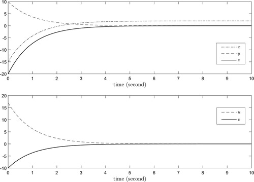
Remark 6.1

It is pointed in Brocket (1983) that for this example system there does not exist a continuous control law which asymptotically stabilises the system at the origin. On one side, the above treatment supports this fact more clearly in two ways. Firstly, the design requires $c_0=\tilde{y}\left(0\right)>0.$ Secondly, note $a_2>0,$ we have from (92(92) $\begin{array}{rl}& \underset{t\to \mathrm{\infty }}{lim}\tilde{x}\left(t\right)\\ & =\left\{\begin{array}{ll}\mathrm{\infty },& \text{ when }{a}_2\le a_1\\ -\frac{a_2{d}_0}{2c_0\left(a_2-a_1\right)}+{\tilde{x}}_0,& \text{ when }{a}_2>a_1,\end{array}\right..\end{array}$(92) ) $\underset{t\to \mathrm{\infty }}{lim}\tilde{x}\left(t\right)\ne 0$ when ${\tilde{x}}_0\ne 0$ and $d_0=\tilde{z}\left(0\right)\ne 0$. While on the other side, the above treatment gives an ‘almost’ globally stabilising controller, with a clearly asymptotical behaviour of all the system variables.

Remark 6.2

We have to mention an important issue, that is, the stability achieved in this example, or generally the stability achieved with the HOFA approaches when the system is sub-fully actuated, is different from the usual definition of stability since constraints on the initial values, for instance, $c_0=\tilde{y}\left(0\right)>0$ in this example system, are often imposed. We remark that this kind of stability is, to an great extent, practically acceptable, and will be further addressed elsewhere.

6.2. Parametric design

Now let us use the second example in Brocket (1983) to demonstrate our parametric design technique for HOFA models.

Example 6.2

Consider the following nonlinear system (Brocket, 1983) (93) $\left\{\begin{array}{l}\dot{x}=u\\ \dot{y}=v\\ \dot{z}=xy.\end{array}\right.$(93) When $y\ne 0,$ we have from the third equation in (93(93) $\left\{\begin{array}{l}\dot{x}=u\\ \dot{y}=v\\ \dot{z}=xy.\end{array}\right.$(93) ) (94) $x=\frac{\dot{z}}{y}.$(94) Taking the derivative of the third equation in (93(93) $\left\{\begin{array}{l}\dot{x}=u\\ \dot{y}=v\\ \dot{z}=xy.\end{array}\right.$(93) ), and using the above relation (94(94) $x=\frac{\dot{z}}{y}.$(94) ), give (95) $\ddot{z}=yu+\frac{\dot{z}}{y}v.$(95) Finally, by combining (95(95) $\ddot{z}=yu+\frac{\dot{z}}{y}v.$(95) ) and the second equation in (93(93) $\left\{\begin{array}{l}\dot{x}=u\\ \dot{y}=v\\ \dot{z}=xy.\end{array}\right.$(93) ), we obtain the following sub-fully actuated model for the system (96) $\left[\begin{array}{c}\ddot{z}\\ \dot{y}\end{array}\right]=\left[\begin{array}{cc}y& \frac{\dot{z}}{y}\\ 0& 1\end{array}\right]\left[\begin{array}{c}u\\ v\end{array}\right],$(96) whose set of feasible points is $\mathbb{F}=\left\{\left.\left[\begin{array}{c}x\\ y\\ z\end{array}\right]\right|y\ne 0\right\}.$Therefore, the system (93(93) $\left\{\begin{array}{l}\dot{x}=u\\ \dot{y}=v\\ \dot{z}=xy.\end{array}\right.$(93) ) is controllable on $\mathbb{F}$.

6.2.1. Control with external inputs

By the decoupled design approach, a controller for the system can be designed as (97) $\begin{array}{rl}\left[\begin{array}{c}u\\ v\end{array}\right]& =-{\left[\begin{array}{cc}y& \frac{\dot{z}}{y}\\ 0& 1\end{array}\right]}^{-1}\\ & \times \left(\left[\begin{array}{c}{a}_{0}z+a_1\dot{z}\\ \text{β}y\end{array}\right]-\left[\begin{array}{c}{u}_0\\ v_0\end{array}\right]\right),\end{array}$(97) where $a_0,a_1$ and β are three scalars, and $u_0$ and $v_0$ are some external inputs. The closed-loop system is (98) $\left\{\begin{array}{l}\ddot{z}+a_1\dot{z}+a_{0}z=u_0\\ \dot{y}+\text{β}y=v_0.\end{array}\right.$(98) Remember that the feasibility condition is $y\left(t\right)\ne 0$. By examining the second equation in (98(98) $\left\{\begin{array}{l}\ddot{z}+a_1\dot{z}+a_{0}z=u_0\\ \dot{y}+\text{β}y=v_0.\end{array}\right.$(98) ), we can easily obtain the following obvious relation (99) $y\left(t\right)\ne 0,\text{ if }y\left(0\right)v_0\left(0\right)>0.$(99) Based on this, the following result for the above design can be immediately obtained.

Proposition 6.3

Let $a_0,a_1$ and β be positive scalars, $u_0\left(t\right)$ and $v_0\left(t\right)$ be continuous and bounded, and $v_0\left(t\right)$ satisfy the following condition (100) $\left|v_0\left(t\right)\right|\ge \gamma ,\mathrm{\forall }t\ge 0,$(100) for some $\gamma >0$. Then the controller (97(97) $\begin{array}{rl}\left[\begin{array}{c}u\\ v\end{array}\right]& =-{\left[\begin{array}{cc}y& \frac{\dot{z}}{y}\\ 0& 1\end{array}\right]}^{-1}\\ & \times \left(\left[\begin{array}{c}{a}_{0}z+a_1\dot{z}\\ \text{β}y\end{array}\right]-\left[\begin{array}{c}{u}_0\\ v_0\end{array}\right]\right),\end{array}$(97) ) is bounded $($feasible$)$ if the initial condition $y_0=y\left(0\right)$ is chosen different from zero and has the same sign as $v_0\left(0\right),$ that is (101) $y_0{v}_0\left(0\right)>0.$(101)

It is understandable that signal tracking can be further easily considered by properly selecting the external signals $u_0\left(t\right)$ and $v_0\left(t\right).$ The above proposition tells us that signal tracking in such a system can be realised ‘almost’ globally. What is more, the system variables y and z are governed by a linear system, while the system variable x given by (94(94) $x=\frac{\dot{z}}{y}.$(94) ) can be easily reasoned to be bounded.

6.2.2. Control without external inputs

In the following, let us consider, as in Brocket (1983), stabilisation of the equilibrium at the origin, hence we assume now $u_0\left(t\right)=v_0\left(t\right)\equiv 0$. In this case the controller (97(97) $\begin{array}{rl}\left[\begin{array}{c}u\\ v\end{array}\right]& =-{\left[\begin{array}{cc}y& \frac{\dot{z}}{y}\\ 0& 1\end{array}\right]}^{-1}\\ & \times \left(\left[\begin{array}{c}{a}_{0}z+a_1\dot{z}\\ \text{β}y\end{array}\right]-\left[\begin{array}{c}{u}_0\\ v_0\end{array}\right]\right),\end{array}$(97) ) turns into (102) $\left\{\begin{array}{l}u=-\frac{1}{y}\left(z{a}_0+\left(a_1-\text{β}\right)\dot{z}\right)\\ v=-y\text{β},\end{array}\right.$(102) and the corresponding closed-loop system becomes (103) $\left\{\begin{array}{l}\ddot{z}+a_1\dot{z}+a_{0}z=0\\ \dot{y}+\text{β}y=0.\end{array}\right.$(103) Without loss of generality, let us make the following assumption.

Assumption A2

The parameters $a_0$ and $a_1$ are so designed that the first equation in system (103(103) $\left\{\begin{array}{l}\ddot{z}+a_1\dot{z}+a_{0}z=0\\ \dot{y}+\text{β}y=0.\end{array}\right.$(103) ) has the solution (104) $z=c_1{\text{e}}^{-t{\alpha }_1}+c_2{\mathrm{e}}^{-t{\alpha }_2},$(104) where $c_1$ and $c_2$ are two scalars, and ${\alpha }_1$ and ${\alpha }_2$ are two distinct positive real scalars.

Under the above assumption, we have the following conclusion.

Proposition 6.4

Let $a_0,a_1$ and β be positive scalars satisfying Assumption A2. Further assume

1. $y\left(0\right)\ne 0,$ and

2. ${\alpha }_i>\text{β}>0,i=1,2,$

then the system variables x, y, z and the controller given in (102(102) $\left\{\begin{array}{l}u=-\frac{1}{y}\left(z{a}_0+\left(a_1-\text{β}\right)\dot{z}\right)\\ v=-y\text{β},\end{array}\right.$(102) ) all converge exponentially to zero.

Proof.

Under Assumption A2, we clearly know that $z\left(t\right)$ converges exponentially to zero. Further, following from the second equation in (103(103) $\left\{\begin{array}{l}\ddot{z}+a_1\dot{z}+a_{0}z=0\\ \dot{y}+\text{β}y=0.\end{array}\right.$(103) ), we have (105) $y=y_0{\mathrm{e}}^{-t\text{β}}.$(105) Therefore, $y\left(t\right)$ converges exponentially to zero in view of $\text{β}>0$.

Since (106) $\dot{z}=-c_1{\alpha }_1{\mathrm{e}}^{-t{\alpha }_1}-c_2{\alpha }_2{\mathrm{e}}^{-t{\alpha }_2},$(106) we have, from (94(94) $x=\frac{\dot{z}}{y}.$(94) ), $x=-\frac{1}{y_0}\left(c_1{\alpha }_1{\mathrm{e}}^{-t\left({\alpha }_1-\text{β}\right)}+c_2{\alpha }_2{\mathrm{e}}^{-t\left({\alpha }_2-\text{β}\right)}\right),$which is also clearly seen to converge exponentially to zero.

Next, let us consider the controller (102(102) $\left\{\begin{array}{l}u=-\frac{1}{y}\left(z{a}_0+\left(a_1-\text{β}\right)\dot{z}\right)\\ v=-y\text{β},\end{array}\right.$(102) ). Using (105(105) $y=y_0{\mathrm{e}}^{-t\text{β}}.$(105) ), we have (107) $v=-y\text{β}=-y_0\text{β}{\mathrm{e}}^{-t\text{β}},$(107) which converges exponentially to zero. Further, using (104(104) $z=c_1{\text{e}}^{-t{\alpha }_1}+c_2{\mathrm{e}}^{-t{\alpha }_2},$(104) ) and (106(106) $\dot{z}=-c_1{\alpha }_1{\mathrm{e}}^{-t{\alpha }_1}-c_2{\alpha }_2{\mathrm{e}}^{-t{\alpha }_2},$(106) ), we can easily derive $\begin{array}{rl}& z{a}_0+\left(a_1-\text{β}\right)\dot{z}\\ & =d_1{\mathrm{e}}^{-t{\alpha }_1}+d_2{\mathrm{e}}^{-t{\alpha }_2},\end{array}$with $\begin{array}{rl}{d}_1& =c_1\left(a_0-\text{β}{\alpha }_1+{\alpha }_1{a}_1\right),\\ d_2& =c_2\left(a_0-\text{β}{\alpha }_2+{\alpha }_2{a}_1\right).\end{array}$Thus (108) $\begin{array}{rl}u& =-\frac{d_1{\mathrm{e}}^{-t{\alpha }_1}+d_2{\mathrm{e}}^{-t{\alpha }_2}}{y_0{\mathrm{e}}^{-t\text{β}}}\\ & =-\frac{1}{y_0}\left(d_1{\mathrm{e}}^{-t\left({\alpha }_1-\text{β}\right)}+d_2{\mathrm{e}}^{-t\left({\alpha }_2-\text{β}\right)}\right),\end{array}$(108) which also goes to zero exponentially. The proof is completed.

For the case of $a_0=6,a_1=5$, and $\text{β}=1,$ simulation of the designed control system has been carried out and shown in Figure 3, where the initial values are taken as $x\left(0\right)=-15,y\left(0\right)=10,z\left(0\right)=-20.$

Figure 3. Simulation results for Example 6.2.

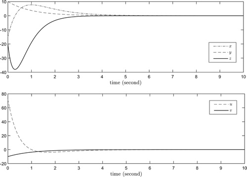
Remark 6.3

In Brocket (1983), a locally stabilising controller for the example system (93(93) $\left\{\begin{array}{l}\dot{x}=u\\ \dot{y}=v\\ \dot{z}=xy.\end{array}\right.$(93) ) is proposed. While Proposition 6.4 tells us that an ‘almost’ globally stabilising controller in fact exists for the system. What is more, the system variables y and z are determined by a stable linear system, and the state x, like y and z, also converges to zero exponentially. We point out that the constraint $y_0\ne 0,$ on the initial value, is not at all strict since initial values of a system can often be altered according to one's will.

Remark 6.4

It is obvious that the system variables x and y are in a symmetry position. In the above design, we have required $y\ne 0,$ and derived a HOFA system with variables y and z. While using this symmetry structure of the system, we can also require $x\ne 0,$ and derive a HOFA system with variables x and z. Combining both cases, we can give a solution to the system under the much weaker condition $x_0^2+y_0^2\ne 0.$

7. Concluding remarks

Nonlinear control system theories based on state-space approaches have appeared more than half a century, and yet systematic and effective methods are still lacking for the various analysis and design problems, including the most basic and crucial problems of controllability analysis and stabilising control.

In the recent two series of papers, Duan (2020a, 2020b, 2020c), and Duan (2020d, 2021a, 2021b, 2021c, 2021d), a different approach other than the state-space approach is proposed, which is termed as the HOFA system approach. In this paper, several aspects of the proposed HOFA approach are further improved and proposed, and by now a relatively more complete general picture of the HOFA system approaches has been roughly sketched.

1. Control systems modelling This physical world is mostly governed by a set of physical laws, such as Newton's Law, Theorems of Linear and Angular Momentum, Lagrangian Equation, and Kirchhoff's Law of Voltage of Current. When modelling using such laws, a set of basic differential equations of second-order are established. Based on this set of second-order basic equations, on one hand a state-space model can be derived if the method of variable extension is applied, while on the other hand a HOFA model may be obtained if the method of variable elimination is applied. It is particularly shown in this paper that a type of general and more meaningful HOFA models with multiple orders exist for general dynamical systems.

2. Control systems analysis Based on the proposed type of general HOFA models, and their superior advantage in control systems design as shown in Duan (2020a, 2021a) and this present paper, controllability of general control systems is defined (originally in Duan, 2020b and modified in this paper). It is further shown in this paper that a general control system can be represented by a controllable subsystem described by a HOFA model, together with an extra uncontrollable one (if exists) or a supplementary one (if exists). Furthermore, a general control system is stabilisable if its uncontrollable (autonomous) subsystem does not exist or is stable in a certain sense, and is strongly stabilisable if a stabilising controller can be designed mainly based on the controllable subsystem described by a HOFA model.

3. Control systems design It is shown that once a general dynamical system is represented via a HOFA model, instead of a state-space one, a controller for the system can be easily designed such that the closed-loop system is a constant linear one with arbitrarily assignable eigenstructure. Two parametric design approaches for the proposed general HOFA models are proposed, which provide all the degrees of freedom to be further utilised to meet other design performance. Based on the proposed general HOFA models with multiple orders, many other control design problems, such as robust control (Duan, 2021c), adaptive control (Duan, 2021d), robust adaptive control (Duan, 2020d), and disturbance rejection (Duan, 2020e), can also be easily treated and better solved.

In addition, the above described HOFA approaches for system analysis and control can also be extended to discrete-time systems, delayed-time systems, stochastic systems and also more complicated systems having mixed features of these mentioned ones.

It is well-known that feedback linearisation is a state-space technique which aims to linearise a nonlinear system by feedback control. By now clear differences between the proposed HOFA approach and the well-known feedback linearisation technique can be readily recognised:

1. the HOFA approach turns out to be a general approach for analysis and control of dynamical systems, while feedback linearisation is only a technique involved in a particular control design problem;

2. the first step of the HOFA approach is to provide a general physical model for a dynamical control system in a HOFA system form, while feedback linearisation is a control technique for a special type of state-space systems;

3. a HOFA model totally reflects the dynamics of the whole physical system, while the result of feedback linearisation generally gives, by its definition, only a part of the system dynamics;

4. the HOFA approach can deal with many sub-fully actuated systems, while the feedback linearisation technique generally can not, and

5. it has been proven that all feedback linearisable state-space systems can be equivalently converted into HOFA models (Duan, 2020a), by effect feedback linearisation may happen to be a very special case in the HOFA approach.

Acknowledgments

The author is grateful to his Ph.D. students Guangtai Tian, Qin Zhao, Xiubo Wang, Weizhen Liu, Kaixin Cui, etc., for helping him with reference selection and proofreading. His particular thanks go to his students Mingzhe Hou, Bin Zhou and Tianyi Zhao for their useful suggestions and help with the examples. Helpful comments from Professor Jun Zhao at the Northeasten University, China, is also very much appreciated.

Disclosure statement

No potential conflict of interest was reported by the author(s).

Additional information

Funding

This work has been partially supported by the Major Program of National Natural Science Foundation of China [grant numbers 61690210, 61690212], the National Natural Science Foundation of China [grant number 61333003] and the Self-Planned Task of State Key Laboratory of Robotics and System (HIT) [grant number SKLRS201716A].

Notes on contributors

Guangren Duan

Guangren Duan received his Ph.D. degree in Control Systems Sciences from Harbin Institute of Technology, Harbin, P. R. China, in 1989. After a two-year post-doctoral experince at the same university, he became professor of control systems theory at that university in 1991. He is the founder and currently the Director of the Center for Control Theory and Guidance Technology at Harbin Institute of Technology. He visited the University of Hull, the University of Sheffield, and also the Queen's University of Belfast, U.K., from December 1996 to October 2002, and has served as Member of the Science and Technology committee of the Chinese Ministry of Education, Vice President of the Control Theory and Applications Committee, Chinese Association of Automation (CAA), and Associate Editors of a few international journals. He is currently an Academician of the Chinese Academy of sciences, and Fellow of CAA, IEEE and IET. His main research interests include parametric control systems design, nonlinear systems, descriptor systems, spacecraft control and magnetic bearing control. He is the author and co-author of 5 books and over 270 SCI indexed publications.

References

- Bellman, R., Bentsman, J., & Meerkov, S. (1986). Vibrational control of nonlinear systems: Vibrational controllability and transient behavior. IEEE Transactions on Automatic Control, 31(8), 717–724. https://doi.org/https://doi.org/10.1109/TAC.1986.1104383
- Brocket, R. W. (1983). Asymptotic stability and feedback stabilization. In Differential geometric control theory (pp. 112–121). Birkhauser.
- Casti, J. L. (1982). Recent development and future perspectives in nonlinear system theory. SIAM Review, 24(3), 301–331. https://doi.org/https://doi.org/10.1137/1024065
- Celikovsky, S. (2000). Local stabilization and controllability of a class of nontriangular nonlinear systems. IEEE Transactions on Automatic Control, 45(10), 1909–1913. https://doi.org/https://doi.org/10.1109/TAC.2000.880997
- Celikovsky, S., & Nijmeijer, H. (1997). On the relation between local controllability and stabilizability for a class of nonlinear systems. IEEE Transactions on Automatic Control, 42(1), 90–94. https://doi.org/https://doi.org/10.1109/9.553690
- Cheng, D. Z., & Qin, H. J. (1987). Geometric methods for nonlinear systems (Part 2): Current dynamics and prospects. Control Theory and Applications, 4(2), 1–9.
- Clarke, F. H., Ledyaev, Y. S., Sontag, E. D., & Subbotin, A. I. (1997). Asymptotic controllability implies feedback stabilization. IEEE Transactions on Automatic Control, 42(10), 1394–1407. https://doi.org/https://doi.org/10.1109/9.633828
- Duan, G. R. (1992). Simple algorithm for robust pole assignment in linear output feedback. IEE Proceedings-Control Theory and Applications, 139(5), 465–470. https://doi.org/https://doi.org/10.1049/ip-d.1992.0058
- Duan, G. R. (1993). Robust eigenstructure assignment via dynamical compensators. Automatica, 29(2), 469–474. https://doi.org/https://doi.org/10.1016/0005-1098(93)90140-O
- Duan, G. R. (2014). Missile attitude control—A direct parametric approach. In The 33rd Chinese Control Conference, Nanjing, China (pp. 28–30). IEEE Press.
- Duan, G. R. (2015). Generalized Sylvester equations: Unified parametric solutions. CRC Press.
- Duan, G. R. (2020a). High-order system approaches: I. Full-actuation and parametric design. Acta Automatica Sinica, 46(7), 1333–1345. https://doi.org/10.16383/j.aas.c200234
- Duan, G. R. (2020b). High-order system approaches: II. Controllability and fully-actuation. Acta Automatica Sinica, 46(8), 1571–1581. https://doi.org/10.1080/00207721.2020.1829168
- Duan, G. R. (2020c). High-order system approaches: III. Observability and observer design. Acta Automatica Sinica, 46(9), 1885–1895. https://doi.org/10.16383/j.aas.c200370
- Duan, G. R. (2020d). High-order fully actuated system approaches: Part V. Robust adaptive control. International Journal of System Sciences. https://doi.org/10.1080/00207721.2021.1879964
- Duan, G. R. (2020e). High-order fully actuated system approaches: Part VI. Disturbance attenuation and decoupling. International Journal of System Sciences. https://doi.org/10.1080/00207721.2021.1879966
- Duan, G. R. (2020f). Quasi-linear system approaches for flight vehicle control – Part 1: An overview and problems. Journal of Astronautics, 41(6), 633–646.
- Duan, G. R. (2021a). High-order fully actuated system approaches: Part I. Models and basic procedure. International Journal of System Sciences, 52(2), 422–435. https://doi.org/10.1080/00207721.2020.1829167
- Duan, G. R. (2021b). High-order fully actuated system approaches: Part II. Generalized strict-feedback systems. International Journal of System Sciences, 52(3), 437–454. https://doi.org/10.1080/00207721.2020.1829168
- Duan, G. R. (2021c). High-order fully actuated system approaches: Part III. Robust control and high-order backstepping. International Journal of System Sciences, 52(5), 952–971. https://doi.org/10.1080/00207721.2020.1849863
- Duan, G. R. (2021d). High-order fully actuated system approaches: Part IV. Adaptive control and high-order backstepping. International Journal of System Sciences, 52(5), 972–989. https://doi.org/10.1080/00207721.2020.1849864
- Duan, G. R., Irwin, G. W., & Liu, G. P. (2002). Disturbance attenuation in linear systems via dynamical compensators: A parametric eigenstructure assignment approach. IEE Proceedings-Control Theory and Applications, 147(2), 129–136. https://doi.org/https://doi.org/10.1049/ip-cta:20000135
- Duan, G. R., Liu, G. P., & Thompson, S. (2000). Disturbance attenuation in Luenberger function observer designs—A parametric approach. IFAC Proceedings Volumes, 33(14), 41–46. https://doi.org/https://doi.org/10.1016/S1474-6670(17)36202-X
- Duan, G. R., & Zhao, T. Y. (2020). Observer-based multi-objective parametric design for spacecraft with super flexible netted antennas. Science China Information Sciences, 63(172002), 1–21. https://doi.org/10.1007/s11432-020-2916-8
- Hanba, S. (2017). Controllability to the origin implies state-feedback stabilizability for discrete-time nonlinear systems. Automatica, 76, 49–52. https://doi.org/https://doi.org/10.1016/j.automatica.2016.09.046
- Jing, Y. W., & Hu, S. Q. (1996). Isomorphic decompositon and controllability of systems possessing solvable general symmetries. Control Theory and Applications, 13(2), 259–263. (in Chinese).
- Kalman, R. E. (1959). On the general theory of control systems. IRE Transactions on Automatic Control, 4(3), 110–110. https://doi.org/https://doi.org/10.1109/TAC.1959.1104873
- Kalman, R. E. (1960). On the general theory of control systems. Proceedings of the 1st IFAC Moscow Congress, 1(1), 491–502. https://doi.org/10.1016/S1474-6670
- Klamka, J. (1975a). Local controllability of perturbed nonlinear systems. IEEE Transactions on Automatic Control, 20(2), 289–291. https://doi.org/https://doi.org/10.1109/TAC.1975.1100929
- Klamka, J. (1975b). Global controllability of perturbed nonlinear systems. IEEE Transactions on Automatic Control, 20(1), 170–172. https://doi.org/https://doi.org/10.1109/TAC.1975.1100870
- Klamka, J. (1976). Relative controllability of nonlinear systems with delays in control. Automatica, 12(6), 633–634. https://doi.org/https://doi.org/10.1016/0005-1098(76)90046-7
- Klein, M. (1990). Mathematical thought from ancient to modern times. Oxford University Press.
- Li, W. L., & Gao, W. B. (1989). Controllability canonical form for nonlinear control systems. Acta Aeronautica ET Astronautica Sinica, 10(5), 249–258.
- Mirza, K., & Womack, B. (1972). Controllability of a class nonlinear systems. IEEE Transactions on Automatic Control, 16(4), 531–535. https://doi.org/https://doi.org/10.1109/TAC.1972.1100043
- Müller, M. A., Liberzon, D., & Allgöwer, F. (2015). Norm-controllability of nonlinear systems. IEEE Transactions on Automatic Control, 60(7), 1825–1840. https://doi.org/https://doi.org/10.1109/TAC.2015.2394953
- Sun, Y. M. (2007). Necessary and sufficient condition for global controllability of planar affine nonlinear systems. IEEE Transactions on Automatic Control, 52(8), 1454–1460. https://doi.org/https://doi.org/10.1109/TAC.2007.902750
- Sun, Y. M. (2010). Further results on global controllability of planar nonlinear systems. IEEE Transactions on Automatic Control, 55(8), 1872–1875. https://doi.org/https://doi.org/10.1109/TAC.2010.2048054
- Tie, L., Cai, K. Y., & Lin, Y. (2011). A survey on the controllability of bilinear systems. Acta Automatica Sinica, 37(9), 1040–1049. https://doi.org/10.3724/SP.J.1004.2011.01040
- Vidyasag, M. (1972). Controllability condition for nonlinear systems. IEEE Transactions on Automatic Control, 17(4), 569–570. https://doi.org/https://doi.org/10.1109/TAC.1972.1100064
- Zheng, Y. F., Willems, J. C., & Zhang, C. H. (2001). A polynomial approach to nonlinear system controllability. IEEE Transactions on Automatic Control, 46(11), 1782–1788. https://doi.org/https://doi.org/10.1109/9.964691