Distributed design for active fault diagnosis

Abstract

The paper deals with active fault diagnosis of stochastic large-scale systems consisting of several subsystems with separate inputs and observations, which are coupled through the system state. The subsystems are described by multiple models expressing their fault-free and faulty behaviour. The transition between the models is governed by a Markov chain. The paper proposes a distributed design of an active fault diagnosis algorithm, which takes into account the coupling among the subsystems in all stages of the algorithm. This results in a higher quality of the excitation signal and consequently in better decisions. The numerical example shows the improved performance of the proposed algorithm in comparison with the algorithms based on the decentralised design.

Keywords:

• Fault diagnosis
• active fault diagnosis
• large-scale systems
• stochastic systems
• multiple models
• distributed architecture

1. Introduction

Complexity and degree of integration of large-scale systems (LSSs) increase their liability to faults with possible catastrophic consequences. Therefore, they have to be detected reliably and as quickly as possible by a fault diagnosis (FD) system. The literature recognises two fundamental approaches that differ in the interaction with the monitored system. In the passive approach (Blanke et al., 2016; Gustafsson, 2009; Isermann, 2011; Katipamula & Brambley, 2011; Yao et al., 2019), the decisions generated by an FD system are based on passive observations of the monitored system measurable quantities. When the active approach is chosen, besides the decisions, the FD system generates an input signal to excite the monitored system (Ashari et al., 2012; Niemann & Poulsen, 2014; Punčochář et al., 2015; Raimondo et al., 2016). Its purpose is to obtain more information, which helps to detect faults that may pose a challenge for the passive FD. The active FD (AFD) approach has gained in popularity in the last decade (Campbell & Nikoukhah, 2004; Heirung & Mesbah, 2019; Niemann, 2006; Paulson et al., 2017; Scott et al., 2014; Stoustrup & Niemann, 2010). Within the AFD for stochastic systems, the multiple-model framework is used almost exclusively to describe fault-free and faulty models of the system (Blackmore et al., 2008; Škach et al., 2016).

Limited communication bandwidth and available computational power are two main reasons for developing special FD algorithms for the LSSs (Ferrari et al., 2012; Raimondo et al., 2016). In Punčochář and Straka (2019) and Straka and Punčochář (2019), a new AFD framework for stochastic LSSs was introduced involving three architectures – centralised, decentralised, and distributed. In the centralised architecture, all calculations are performed by a single central node, while in the decentralised architecture, the calculations are performed by multiple isolated nodes each tied to a single LSS subsystem. The distributed architecture is similar to the decentralised one and in addition, the nodes communicate with each other. The AFD algorithms consist of (i) the off-line stage, dealing with the design of the excitation input and decision generators, and (ii) the on-line stage, dealing with the state estimation and utilisation of the designed generators. The LSS consists of several subsystems which are subject to certain dynamic interactions called coupling. The input generator design cannot respect the coupling among the LSS subsystems fully for computational tractability reasons even for small-scale systems¹. To achieve reasonable computational costs of the AFD algorithm, the input generator design introduced in Punčochář and Straka (2019) and Straka and Punčochář (2019) rested on the decentralised architecture, which completely ignores the coupling. This, however, leads to lower quality of the excitation and consequently to lower quality of the FD.

This paper makes the following contribution: A novel distributed AFD algorithm is designed to take into account the coupling among the LSS subsystems in both stages. Compared to the AFD algorithm proposed by Straka and Punčochář (2019), where the AFD node related to a subsystem uses the information received from other nodes in the on-line stage only, the novelty of the AFD algorithm proposed here lies in the off-line stage where the input signal generator is designed. In the proposed distributed AFD algorithm, the input signal generator related to a subsystem employs conveniently the information about the state of other subsystems to take into account the subsystem coupling. The contribution of the paper lies in a convenient aggregation of the effects of other subsystems (i.e. compressing the information) to achieve feasible computational costs. Note that using the information in the uncompressed form would lead to extreme computational costs of the centralised architecture. The additional information available to the generator improves the quality of the excitation input and consequently the quality of the FD.

The paper is structured as follows: Section 2 provides the LSS specification, decomposition, and the AFD problem formulation. A general solution to the AFD problem is briefly summarised in Section 3. The distributed design for the AFD is proposed in Section 4. The performance of the proposed algorithm is illustrated using two numerical examples in Section 5 and Section 6 draws concluding remarks.

2. AFD problem formulation

2.1. LSS specification

Consider an LSS Σ described at time instant $k\in \mathcal{T}=\{0,1,2,\dots \}$ by the following state-space model (1a) $\begin{array}{rl}\mathrm{\Sigma }:{\mathbf{x}}_{k+1}& =\mathbf{f}({\mathbf{x}}_k,{\mathit{\mu }}_k,{\mathbf{u}}_k)+\mathbf{F}({\mathit{\mu }}_k){\mathbf{w}}_k,\end{array}$(1a) (1b) $\begin{array}{rl}{\mathbf{y}}_k& =\mathbf{h}({\mathbf{x}}_k,{\mathit{\mu }}_k)+\mathbf{H}({\mathit{\mu }}_k){\mathbf{v}}_k,\end{array}$(1b) where ${\mathbf{x}}_k\in \mathcal{X}\subseteq {\mathbb{R}}^{D_x}$ and ${\mathit{\mu }}_k\in \mathcal{M}$ are the continuous and discrete parts of the LSS state ${\mathbf{s}}_k=[{\mathbf{x}}_k^{\mathrm{T}},{\mathit{\mu }}_k^{\mathrm{T}}{]}^{\mathrm{T}}\in \mathcal{S}=\mathcal{X}\times \mathcal{M}$, ${\mathbf{u}}_k\in \mathcal{U}\subseteq {\mathbb{R}}^{D_u}$ is the input, ${\mathbf{w}}_k\in \mathcal{X}$ is the state noise described by the known probability density function (PDF) $p_{{\mathbf{w}}_k}$, ${\mathbf{y}}_k\in \mathcal{Y}\subseteq {\mathbb{R}}^{D_y}$ is the output, and ${\mathbf{v}}_k\in \mathcal{Y}$ is the measurement noise described by the known PDF $p_{{\mathbf{v}}_k}$. The functions $\mathbf{f}:\mathcal{X}\times \mathcal{M}\times \mathcal{U}\mapsto \mathcal{X}$, $\mathbf{h}:\mathcal{X}\times \mathcal{M}\mapsto \mathcal{Y}$, $\mathbf{F}:\mathcal{M}\mapsto \mathcal{X}\times \mathcal{X}$, and $\mathbf{H}:\mathcal{M}\mapsto \mathcal{Y}\times \mathcal{Y}$ are known². Each element ${\mathit{\mu }}_k$ of the discrete set $\mathcal{M}$ represents a multi-index into a set of M possible models describing behaviour of the LSS Σ in the fault-free and faulty conditions during a sampling period. The random process $\{{\mathit{\mu }}_k\}$ is assumed to be Markov with known transition probability (2) $Pr({\mathit{\mu }}_{k+1}|{\mathit{\mu }}_k).$(2) The state and measurement noises are white, mutually independent and independent of the initial condition ${\mathbf{s}}_0$ described by $p_{{\mathbf{s}}_0}$ so that³ (3) $p({\mathbf{w}}_{0:F},{\mathbf{v}}_{0:F},{\mathbf{s}}_0)=p_{{\mathbf{s}}_0}({\mathbf{s}}_0)\prod _{k=0}^F{p}_{{\mathbf{w}}_k}({\mathbf{w}}_k)p_{{\mathbf{v}}_k}({\mathbf{v}}_k)$(3) for any $F\in \mathcal{T}$. Both the continuous part ${\mathbf{x}}_k$ of the state ${\mathbf{s}}_k$ and the discrete part ${\mathit{\mu }}_k$ are unknown and can be inferred indirectly through available ${\mathbf{y}}_k$ and ${\mathbf{u}}_k$.

2.2. LSS decomposition

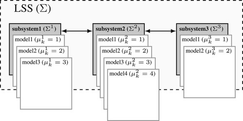
Since the AFD for the LSS Σ with a centralised architecture is not computationally tractable⁴, the decentralised or distributed architectures based on a decomposition of Σ were considered in Punčochář Straka (2019); Straka Punčochář (2019). The LSS Σ (see Figure 1) consists of N subsystems⁵ ${\mathrm{\Sigma }}^n,n\in \mathcal{N}=\{1,2,\dots ,N\}$ that are coupled through the state⁶ ${\mathbf{x}}_k$. Each subsystem ${\mathrm{\Sigma }}^n$ has its own inputs ${\mathbf{u}}_k^n$, outputs ${\mathbf{y}}_k^n$, and a set of possible fault-free and faulty models ${\mathcal{M}}^n$. It can be described by the following representation (4a) $\begin{array}{rl}& {\mathrm{\Sigma }}^n:{\mathbf{x}}_{k+1}^n={\mathbf{f}}^n({\mathbf{x}}_k,{\mu }_k^n,{\mathbf{u}}_k^n)+{\mathbf{F}}^n({\mu }_k^n){\mathbf{w}}_k^n,\end{array}$(4a) (4b) $\begin{array}{rl}& Pr({\mu }_{k+1}^n|{\mu }_k^n)\end{array}$(4b) (4c) $\begin{array}{rl}& {\mathbf{y}}_k^n={\mathbf{h}}^n({\mathbf{x}}_k^n,{\mu }_k^n)+{\mathbf{H}}^n({\mu }_k^n){\mathbf{v}}_k^n,\end{array}$(4c) where ${\mathbf{x}}_k^n\in {\mathcal{X}}^n\subseteq {\mathbb{R}}^{D_x^n}$ and ${\mu }_k^n\in {\mathcal{M}}^n=\{1,2,\dots ,M^n\}$ are continuous and discrete parts, respectively, of the local state⁷ ${\mathbf{s}}_k^n=[({\mathbf{x}}_k^n{)}^{\mathrm{T}},{\mu }_k^n{]}^{\mathrm{T}}\in {\mathcal{S}}^n={\mathcal{X}}^n\times {\mathcal{M}}^n$ of the subsystem ${\mathrm{\Sigma }}^n$, ${\mathbf{u}}_k^n\in {\mathcal{U}}^n\subseteq {\mathbb{R}}^{D_u^n}$ is the local input, ${\mathbf{w}}_k^n\in {\mathcal{X}}^n$ is the local state noise described by $p_{{\mathbf{w}}_k^n}$, ${\mathbf{y}}_k^n\in {\mathcal{Y}}^n\subseteq {\mathbb{R}}^{D_y^n}$ is the local output, ${\mathbf{v}}_k^n\in {\mathcal{Y}}^n$ is the local measurement noise described by $p_{{\mathbf{v}}_k^n}$. The functions ${\mathbf{f}}^n:\mathcal{X}\times {\mathcal{M}}^n\times {\mathcal{U}}^n\mapsto {\mathcal{X}}^n$, ${\mathbf{h}}^n:{\mathcal{X}}^n\times {\mathcal{M}}^n\mapsto {\mathcal{Y}}^n$, ${\mathbf{F}}^n:{\mathcal{M}}^n\mapsto {\mathcal{X}}^n\times {\mathcal{X}}^n$, and ${\mathbf{H}}^n:{\mathcal{M}}^n\mapsto {\mathcal{Y}}^n\times {\mathcal{Y}}^n$ are known. The discrete part ${\mu }_k^n$ represents an index into the set ${\mathcal{M}}^n$, which includes one model representing the behaviour of subsystem ${\mathrm{\Sigma }}^n$ in fault-free condition, ${\mu }_k^n=1$, and $M^n-1$ models that represent the behaviour of subsystem in faulty conditions, ${\mu }_k^n\in \{2,\dots ,M^n\}$.The LSS Σ given by (1a(1a) $\begin{array}{rl}\mathrm{\Sigma }:{\mathbf{x}}_{k+1}& =\mathbf{f}({\mathbf{x}}_k,{\mathit{\mu }}_k,{\mathbf{u}}_k)+\mathbf{F}({\mathit{\mu }}_k){\mathbf{w}}_k,\end{array}$(1a) ) and (2(2) $Pr({\mathit{\mu }}_{k+1}|{\mathit{\mu }}_k).$(2) ) is assumed to satisfy the following independence conditions:

(IC-1)	The initial states ${\mathbf{x}}_0^n$ and the initial model indices ${\mu }_0^n$ are independent and mutually independent8, i.e. $p({\mathbf{x}}_0,{\mathit{\mu }}_0)=\prod _{n=1}^N{p}_{{\mathbf{x}}_0^n}({\mathbf{x}}_0^n)Pr({\mu }_0^n)$.
(IC-2)	The model indices ${\mu }_k^n$ are conditionally independent, i.e. $Pr({\mathit{\mu }}_{k+1}|{\mathit{\mu }}_k)=\prod _{n=1}^{N}Pr({\mu }_{k+1}^n|{\mu }_k^n)$.

Figure 1. The decomposition of an LSS into interconnected subsystems.

The independence conditions IC-1 and IC-2 mean that the occurrence of a fault in a subsystem does not influence the occurrence of faults in other subsystems. The condition IC-2 is considered for convenience purposes only to make the exposition clear. Note that the AFD problem with coupled faults was treated in Straka and Punčochář (2020b) for conditionally dependent faults and in Straka and Punčochář (2020c) for dependent faults. Relaxation of IC-2 would lead to an introduction of a central node in the on-line stage, whereas the off-line stage would not be affected.

In this paper, the subsystems are coupled only through the continuous state ${\mathbf{x}}_k$ that appears in the dynamics (4a(4a) $\begin{array}{rl}& {\mathrm{\Sigma }}^n:{\mathbf{x}}_{k+1}^n={\mathbf{f}}^n({\mathbf{x}}_k,{\mu }_k^n,{\mathbf{u}}_k^n)+{\mathbf{F}}^n({\mu }_k^n){\mathbf{w}}_k^n,\end{array}$(4a) ) of all subsystems, i.e. besides ${\mathbf{x}}_k^n$, the local continuous state ${\mathbf{x}}_{k+1}^n$ is affected by the local continuous states of other subsystems ${\mathbf{x}}_k^{\overline{n}}=[({\mathbf{x}}_k^1{)}^{\mathrm{T}},\dots ,({\mathbf{x}}_k^{n-1}{)}^{\mathrm{T}},({\mathbf{x}}_k^{n+1}{)}^{\mathrm{T}},\dots ,({\mathbf{x}}_k^N{)}^{\mathrm{T}}{]}^{\mathrm{T}}$. The AFD algorithm proposed in Punčochář and Straka (2019) approximated the dynamics (4a(4a) $\begin{array}{rl}& {\mathrm{\Sigma }}^n:{\mathbf{x}}_{k+1}^n={\mathbf{f}}^n({\mathbf{x}}_k,{\mu }_k^n,{\mathbf{u}}_k^n)+{\mathbf{F}}^n({\mu }_k^n){\mathbf{w}}_k^n,\end{array}$(4a) ) by neglecting the coupling through ${\mathbf{x}}_k$ in both stages and the AFD algorithm proposed in Straka and Punčochář (2019) neglected the coupling through ${\mathbf{x}}_k$ in the off-line stage, where the input signal generator is designed. Such approximation is acceptable if the coupling is weak, in which case the approximation has little effect on the FD quality. However, when the coupling is stronger⁹, it should be taken into account by both stages of the AFD design at least to a certain extent. Hence, the paper focuses on the distributed design that considers the coupling.

2.3. AFD problem

For convenience, the AFD problem and its general solution are described for the centralised architecture only. The AFD strives to design a function that transforms the complete available information observed up to the time step k to a decision ${\mathbf{d}}_k$ about the faults (subsystem models) and to an input signal ${\mathbf{u}}_k$, which role is to excite the system to improve the detection quality. The AFD system can be described at any time instant as (5) $\mathrm{\Delta }:\left[\begin{array}{c}{\mathbf{d}}_k\\ {\mathbf{u}}_k\end{array}\right]=\left[\begin{array}{c}{\mathit{\sigma }}_k\left({\mathbf{I}}_k\right)\\ {\mathit{\gamma }}_k\left({\mathbf{I}}_k\right)\end{array}\right],$(5) where ${\mathbf{I}}_k=[{\mathbf{y}}_{0:k}^{\mathrm{T}},{\mathbf{u}}_{0:k-1}^{\mathrm{T}}{]}^{\mathrm{T}}\in {\mathcal{I}}_{0:k}={\mathcal{Y}}^{k+1}\times {\mathcal{U}}^k$. The vector ${\mathbf{d}}_k=[d_k^1,d_k^2,\dots ,d_k^N{]}^{\mathrm{T}}\in \mathcal{M}$ consists of the decisions $d_k^n\in {\mathcal{M}}^n$ about the model indices ${\mu }_k^n$, ${\mathit{\sigma }}_k:{\mathcal{I}}_{0:k}\mapsto \mathcal{M}$ represents the AFD node decision generator at the time step k, ${\mathbf{u}}_k$ is the excitation input and ${\mathit{\gamma }}_k:{\mathcal{I}}_{0:k}\mapsto \mathcal{U}$ is a function describing the input signal generator. Note that by providing the decision ${\mathbf{d}}_k$, the AFD performs the fault detection and the fault identification simultaneously.

The optimal AFD system should minimise the following additive discounted criterion¹⁰ (6) $J({\mathit{\sigma }}_0^{\mathrm{\infty }},{\mathit{\gamma }}_0^{\mathrm{\infty }})=\underset{F\to \mathrm{\infty }}{lim}\mathrm{E}\{\sum _{k=0}^F{\eta }^{k}L({\mathit{\mu }}_k,{\mathbf{d}}_k)\},$(6) where $\eta \in (0,1)$ is a chosen discount factor and $L:\mathcal{M}\times \mathcal{M}\mapsto {\mathbb{R}}^{+}$ is a detection cost function that allows different costs to be assigned for selecting the vector of decisions ${\mathbf{d}}_k$ while the LSS behaviour is currently governed by the vector of model indices ${\mathit{\mu }}_k$. The cost function is versatile and may stress the cost of missed detections or false alerts or even the cost of incorrect fault identification. This paper assumes that the costs are not related across the subsystems, and thus the following additive detection cost function¹¹ is used (7) $L({\mathit{\mu }}_k,{\mathbf{d}}_k)=\sum _{n=1}^N{L}^n({\mu }_k^n,d_k^n),$(7) where $L^n:{\mathcal{M}}^n\times {\mathcal{M}}^n\mapsto {\mathbb{R}}^{+}$ penalises discrepancy between the model index ${\mu }_k^n$ and the decision $d_k^n$ generated by the AFD system.

For an example of two models, if missed detection (${\mu }_k^n=2$, $d_k^n=1$) and false alert (${\mu }_k^n=1$, $d_k^n=2$) are perceived as equally bad by a designer, it is common to choose $L^n({\mu }_k^n,d_k^n)=1-{\delta }_{{\mu }_k^n,d_k^n}$, where ${\delta }_{i,j}$ is the Kronecker delta. On the other hand, if a missed detection has more serious consequences compared to a false alarm, the choice $L^n({\mu }_k^n,d_k^n)=\{\begin{array}{ll}{10}^2& {\mu }_k^n=2,d_k^n=1\\ 1& {\mu }_k^n=1,d_k^n=2\\ 0& {\mu }_k^n=d_k^n\end{array}$specifies the cost of the missed detection by several orders of magnitude higher than the cost of the false alert (Nelles, 2014).

3. General solution to AFD problem

The AFD problem formulation presented in the previous section belongs to the class of imperfect state information problems as only the history ${\mathbf{I}}_k$ is available for control or decision making instead of the state ${\mathbf{s}}_k$ (Bertsekas, 2000). These problems are difficult to address directly for the infinite time horizon as the dimension of ${\mathbf{I}}_k$ increases without limit. A solution is to assume that the optimal AFD node can be split into an optimal state estimator that uses the Bayesian recursive relations (Bar-Shalom et al., 2001) to compute a conditional PDF $p({\mathbf{s}}_k|{\mathbf{I}}_k)$ and a decision-making law that maps this conditional PDF into the input ${\mathbf{u}}_k$ and decision ${\mathbf{d}}_k$ (Bertsekas, 2000; Bertsekas & Shreve, 1996). Given the optimal state estimator, the original problem can be recast as a perfect state information problem where only the decision-making law is to be designed based on a new model consisting of the original model coupled with the optimal state estimator.

The conditional PDF $p({\mathbf{s}}_k|{\mathbf{I}}_k)$ calculated by the state estimator can be represented exactly or approximately using a finite number of statistics. The statistics collected into an information state ${\mathit{\xi }}_k\in \mathcal{K}$ evolve in time as (8) ${\mathit{\xi }}_{k+1}=\mathit{\varphi }({\mathit{\xi }}_k,{\mathbf{u}}_k,{\mathbf{y}}_{k+1}),$(8) where $\mathit{\varphi }:\mathcal{K}\times \mathcal{U}\times \mathcal{Y}\mapsto \mathcal{K}$ represents the state estimator associated with the LSS Σ model. Here, the future output ${\mathbf{y}}_{k+1}$ is regarded as a random disturbance described by the conditional PDF $p({\mathbf{y}}_{k+1}|{\mathbf{I}}_k,{\mathbf{u}}_k)$ and the initial condition ${\mathit{\xi }}_0$ contains statistics describing the conditional PDF $p({\mathbf{s}}_0|{\mathbf{y}}_0)$.

Given the information state ${\mathit{\xi }}_k$, it suffices to consider a time invariant AFD node that is described at a time step $k\in \mathcal{T}$ as (9) $\mathrm{\Delta }:\left[\begin{array}{c}{\mathbf{d}}_k\\ {\mathbf{u}}_k\end{array}\right]=\left[\begin{array}{c}\overline{\mathit{\sigma }}({\mathit{\xi }}_k)\\ \overline{\mathit{\gamma }}({\mathit{\xi }}_k)\end{array}\right],$(9) where $\overline{\mathit{\sigma }}:\mathcal{K}\mapsto \mathcal{M}$ and $\overline{\mathit{\gamma }}:\mathcal{K}\mapsto \mathcal{U}$ are unknown functions to be sought. The detection cost function for the perfect state information model equivalent to L in (6(6) $J({\mathit{\sigma }}_0^{\mathrm{\infty }},{\mathit{\gamma }}_0^{\mathrm{\infty }})=\underset{F\to \mathrm{\infty }}{lim}\mathrm{E}\{\sum _{k=0}^F{\eta }^{k}L({\mathit{\mu }}_k,{\mathbf{d}}_k)\},$(6) ) can be shown (Bertsekas, 2000) to satisfy (10) $\overline{L}({\mathit{\xi }}_k,{\mathbf{d}}_k)=\sum _{n=1}^N\sum _{{\mu }_k^n}{L}^n({\mu }_k^n,d_k^n)Pr({\mu }_k^n|{\mathbf{I}}_k).$(10) Having the reformulated problem specification, the optimal AFD node is determined by the Bellman function, which can be computed off-line (Straka & Punčochář, 2019) because it depends only on the a priori known PDF $p({\mathbf{x}}_{k+1}|{\mathbf{x}}_k,{\mathit{\mu }}_k,{\mathbf{u}}_k)$, transition probabilities $Pr({\mathit{\mu }}_{k+1}|{\mathit{\mu }}_k)$, measurement PDF $p({\mathbf{y}}_k|{\mathbf{x}}_k,{\mathit{\mu }}_k)$, cost function $L^{\mathrm{d}}$, and the discount factor η. Then, the optimal decisions and optimal inputs can be determined on-line by solving much simpler optimisation problems. More precisely, the Bellman function is required for the optimal input signal generator ${\mathbf{u}}_k={\overline{\mathit{\gamma }}}^{\ast }({\mathit{\xi }}_k)$ while the optimal decision generator ${\mathbf{d}}_k={\overline{\mathit{\sigma }}}^{\ast }({\mathit{\xi }}_k)$ works independently of the Bellman function (Straka & Punčochář, 2019). Thus, the AFD algorithm consists of two stages: the off-line stage involved with the design of the input signal generator, which uses the Bellman function, and the on-line stage connected with the state estimation, which generates the decisions and selects the optimal excitation according to the Bellman function.

The computation costs of the Bellman function calculation are extreme for LSSs as the dimension of the information state ${\mathit{\xi }}_k$ can be very high even for low-dimensional state ${\mathbf{s}}_k$ due to the number of subsystems and their models. Consider, for example, an LSS with N subsystems each described by $M^n=2$ models (one model for fault-free behaviour and one model for faulty behaviour). It leads to N-dimensional index ${\mathit{\mu }}_k$ and the information state ${\mathit{\xi }}_k$ consists of $2^N$ statistics of $p({\mathbf{x}}_k^n|{\mu }_k^n,{\mathbf{I}}_k,)$ and $2^N-1$ probabilities $Pr({\mu }_k^n|{\mathbf{I}}_k)$.

For this reason, the input signal generator design proposed in Punčochář and Straka (2019) and Straka and Punčochář (2019) uses solely the decentralised architecture¹², which ignores the coupling among the subsystems and calculates the Bellman function for each subsystem separately using approximate models that are mutually isolated. Thus, each subsystem has its own information state of a significantly smaller dimension than the LSS information state and the computation of the Bellman function related to the subsystem is tractable.

The aim of the distributed design proposed in this paper is to take into account the coupling of the subsystems during the design of the input generator. Thus, the quality of the excitation signal and subsequently of the detection should be improved by using more information from other subsystems that are available in the distributed architecture. Such design comes with lower computational costs than the centralised design.

4. AFD with distributed design

The main idea of the AFD with distributed design is that the information about the LSS state communicated among the AFD nodes will be used not only to generate the decision (Straka & Punčochář, 2019) but also to generate the excitation input.

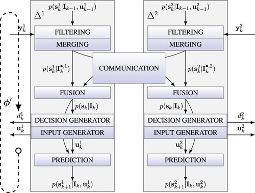
Distributed state estimation: First, the perfect state information model is constructed for the distributed architecture. The estimation algorithm in each AFD node ${\mathrm{\Delta }}^n$ consists of four steps (Straka & Punčochář,2019):

• Prediction – calculation of $p({\mathbf{s}}_k^n|{\mathbf{I}}_{k-1},{\mathbf{u}}_{k-1}^n)$;

• Filtering – calculation of $\overline{p}({\mathbf{s}}_k^n|{\mathbf{I}}_k^{\bullet ,n})$;

• Merging – calculation of the approximation $p({\mathbf{s}}_k^n|{\mathbf{I}}_k^{\bullet ,n})$ of the filtering PDF $\overline{p}({\mathbf{s}}_k^n|{\mathbf{I}}_k^{\bullet ,n})$ to prevent the computational and memory costs increase; and

• Fusion – calculation of $p({\mathbf{s}}_k|{\mathbf{I}}_k)$ by fusing¹³ the filtering estimates received from other nodes.

The symbol ${\mathbf{I}}_k^{\bullet ,n}$ denotes a composition of the past global¹⁴ data ${\mathbf{I}}_{k-1}$ related to the whole system Σ and the present data ${\mathbf{y}}_k^n$, and ${\mathbf{u}}_{k-1}^n$ related to the subsystem ${\mathrm{\Sigma }}^n$ only, i.e. (11) ${\mathbf{I}}_k^{\bullet ,n}=[({\mathbf{I}}_{k-1}{)}^{\mathrm{T}},({\mathbf{y}}_k^n{)}^{\mathrm{T}},({\mathbf{u}}_{k-1}^n{)}^{\mathrm{T}}{]}^{\mathrm{T}}.$(11) The estimation algorithm is illustrated in Figure 2 for two nodes ${\mathrm{\Delta }}^1$ and ${\mathrm{\Delta }}^2$.The dashed arrow loop represents the estimation algorithm, which can be expressed using the perfect state information model as (12) ${\mathit{\xi }}_{k+1}={\mathit{\varphi }}^{\prime }({\mathit{\xi }}_k,{\mathbf{u}}_k,{\mathbf{y}}_{k+1}),$(12) where ${\mathit{\varphi }}^{\prime }:\mathcal{K}\times \mathcal{U}\times \mathcal{Y}\mapsto \mathcal{K}$ differs from $\mathit{\varphi }$ in (8(8) ${\mathit{\xi }}_{k+1}=\mathit{\varphi }({\mathit{\xi }}_k,{\mathbf{u}}_k,{\mathbf{y}}_{k+1}),$(8) ) because the filtering, merging, and prediction steps are performed locally at the AFD node level.

Figure 2. Scheme of distributed AFD algorithm.

Distributed AFD node : Two problems are associated with the model (12(12) ${\mathit{\xi }}_{k+1}={\mathit{\varphi }}^{\prime }({\mathit{\xi }}_k,{\mathbf{u}}_k,{\mathbf{y}}_{k+1}),$(12) ). First, the dimension of the information state ${\mathit{\xi }}_k$ is too large for the Bellman function calculation. Second, the Bellman function calculation for the nth node ${\mathrm{\Delta }}^n$ requires running the estimation algorithms for all subsystems. The first problem will be addressed by aggregating the effects of other subsystems to reduce the order of the statistic. The second problem will be dealt with by a suitable global model approximation.

4.1. Reducing model order by aggregation

The dimension of the statistic ${\mathit{\xi }}_k$ can be reduced if the dynamics function of each subsystem ${\mathrm{\Sigma }}^n$ can be decomposed as (13) ${\mathbf{f}}^n({\mathbf{x}}_k,{\mu }_k^n,{\mathbf{u}}_k^n)={\mathbf{g}}^n({\mathbf{x}}_k^n,{\mu }_k^n,{\mathbf{u}}_k^n,{\mathbf{a}}^n({\mathbf{x}}_k^{\overline{n}},{\mu }_k^n)),$(13) where ${\mathbf{a}}^n:{\mathcal{X}}^{\overline{n}}\times {\mathcal{M}}^n\mapsto {\mathcal{Z}}^n={\mathbb{R}}^{D_z^n}$ is a function that aggregates the effects of other subsystems ${\mathrm{\Sigma }}^1\cdots {\mathrm{\Sigma }}^{n-1},{\mathrm{\Sigma }}^{n+1}\cdots {\mathrm{\Sigma }}^N$ on the subsystem ${\mathrm{\Sigma }}^n$, and ${\mathbf{g}}^n:{\mathcal{X}}^n\times {\mathcal{M}}^n\times {\mathcal{U}}^n\times {\mathcal{Z}}^n\mapsto {\mathcal{X}}^n$ is a function that combines this aggregated effect with the local effects of ${\mathrm{\Sigma }}^n$. A reduced order form of the model (4a(4a) $\begin{array}{rl}& {\mathrm{\Sigma }}^n:{\mathbf{x}}_{k+1}^n={\mathbf{f}}^n({\mathbf{x}}_k,{\mu }_k^n,{\mathbf{u}}_k^n)+{\mathbf{F}}^n({\mu }_k^n){\mathbf{w}}_k^n,\end{array}$(4a) ) for the subsystem ${\mathrm{\Sigma }}^n$ can be written as (14a) $\begin{array}{rl}& {\mathbf{x}}_{k+1}^n={\mathbf{g}}^n({\mathbf{x}}_k^n,{\mu }_k^n,{\mathbf{u}}_k^n,{\mathbf{z}}_k^n)+{\mathbf{F}}^n({\mu }_k^n){\mathbf{w}}_k^n,\end{array}$(14a) (14b) $\begin{array}{rl}& Pr({\mu }_{k+1}^n|{\mu }_k^n),\end{array}$(14b) (14c) $\begin{array}{rl}& {\mathbf{y}}_k^n={\mathbf{h}}^n({\mathbf{x}}_k^n,{\mu }_k^n)+{\mathbf{H}}^n({\mu }_k^n){\mathbf{v}}_k^n,\end{array}$(14c) where ${\mathbf{z}}_k^n\in {\mathcal{Z}}^n$ is a new $D_z^n$-dimensional random variable defined as (15) ${\mathbf{z}}_k^n={\mathbf{a}}^n({\mathbf{x}}_k^{\overline{n}},{\mu }_k^n).$(15) Note that the dimension of all arguments of the function ${\mathbf{a}}^n$ is $D_x^{\overline{n}}+1$ and a reduction of the dimension is actually achieved only if $D_z^n$ is less than $D_x^{\overline{n}}+1$ for all subsystems.

Typical examples of subsystem dynamics that are particularly suitable in this regard are additive models. A nonlinear additive model has the following structure (16) $\begin{array}{rl}{\mathbf{f}}^n({\mathbf{x}}_k,{\mu }_k^n,{\mathbf{u}}_k^n)& ={\mathbf{g}}^n({\mathbf{x}}_k^n,{\mu }_k^n,{\mathbf{u}}_k^n,{\mathbf{a}}^n({\mathbf{x}}_k^{\overline{n}},{\mu }_k^n))\end{array}$(16) (17) $\begin{array}{rl}& ={\mathbf{q}}^n({\mathbf{x}}_k^n,{\mu }_k^n,{\mathbf{u}}_k^n)+{\mathbf{a}}^n({\mathbf{x}}_k^{\overline{n}},{\mu }_k^n),\end{array}$(17) where ${\mathbf{q}}^n:{\mathcal{X}}^n\times {\mathcal{M}}^n\times {\mathcal{U}}^n\mapsto {\mathcal{X}}^n$ represents the local effect and ${\mathbf{a}}^n$ with $D_z^n=D_x^n$ aggregates effect of other subsystems. The additive linear model has an even simpler structure (18) $\begin{array}{rl}{\mathbf{f}}^n({\mathbf{x}}_k,{\mu }_k^n,{\mathbf{u}}_k^n)& =\underset{{\mathbf{q}}^n({\mathbf{x}}_k^n,{\mu }_k^n,{\mathbf{u}}_k^n)}{\underbrace{{\mathbf{A}}_n^n({\mu }_k^n){\mathbf{x}}_k^n+{\mathbf{B}}^n({\mu }_k^n){\mathbf{u}}_k^n}}\\ & +\underset{{\mathbf{a}}^n({\mathbf{x}}_k^{\overline{n}},{\mu }_k^n)}{\underbrace{\sum _{i\in {\mathcal{N}}^{\overline{n}}}{\mathbf{A}}_i^n({\mu }_k^n){\mathbf{x}}_k^i}},\end{array}$(18) where ${\mathcal{N}}^{\overline{n}}=\mathcal{N}\setminus \{n\}$, ${\mathbf{A}}_i^n({\mu }_k^n)\in {\mathbb{R}}^{D_x^n\times D_x^i}$, $i\in \mathcal{N}$ and ${\mathbf{B}}^n({\mu }_k^n)\in {\mathbb{R}}^{D_x^n\times D_u^n}$ are matrices related to the subsystem ${\mathrm{\Sigma }}^n$. The linear additive model is attractive especially from a computational point of view because having the Gaussian conditional PDF of ${\mathbf{x}}_k^{\overline{n}}$, the aggregated effect (19) ${\mathbf{a}}^n({\mathbf{x}}_k^{\overline{n}},{\mu }_k^n)=\sum _{i\in {\mathcal{N}}^{\overline{n}}}{\mathbf{A}}_i^n({\mu }_k^n){\mathbf{x}}_k^i$(19) can be represented exactly by the mean and covariance matrix for each ${\mu }_k^n\in {\mathcal{M}}^n$.

To complete the model (14a(14a) $\begin{array}{rl}& {\mathbf{x}}_{k+1}^n={\mathbf{g}}^n({\mathbf{x}}_k^n,{\mu }_k^n,{\mathbf{u}}_k^n,{\mathbf{z}}_k^n)+{\mathbf{F}}^n({\mu }_k^n){\mathbf{w}}_k^n,\end{array}$(14a) ), the dynamics for the new random variable ${\mathbf{z}}_k^n$ could be defined using (15(15) ${\mathbf{z}}_k^n={\mathbf{a}}^n({\mathbf{x}}_k^{\overline{n}},{\mu }_k^n).$(15) ) and the dynamics of other subsystems. Nevertheless, it is more convenient to consider the conditional PDF $p({\mathbf{x}}_k^n,{\mu }_k^n,{\mathbf{z}}_k^n|{\mathbf{I}}_k)$, which can be obtained from $p({\mathbf{x}}_k,{\mu }_k^n|{\mathbf{I}}_k)$ using (15(15) ${\mathbf{z}}_k^n={\mathbf{a}}^n({\mathbf{x}}_k^{\overline{n}},{\mu }_k^n).$(15) ). The evolution of the conditional PDF $p({\mathbf{x}}_k^n,{\mu }_k^n,{\mathbf{z}}_k^n|{\mathbf{I}}_k)$ can be described by the following model (20) $\begin{array}{rl}& p({\mathbf{x}}_{k+1}^n,{\mu }_{k+1}^n,{\mathbf{z}}_{k+1}^n|{\mathbf{I}}_{k+1})\\ & ={\mathit{\phi }}_{\mathrm{DIS}}(p({\mathbf{x}}_k^n,{\mu }_k^n,{\mathbf{z}}_k^n|{\mathbf{I}}_k),{\mathbf{u}}_k,{\mathbf{y}}_{k+1}),\end{array}$(20) where ${\mathit{\phi }}_{\mathrm{DIS}}:\mathcal{P}\times \mathcal{U}\times \mathcal{Y}\mapsto \mathcal{P}$ is a mapping that encapsulates the distributed estimation algorithm and the model of the LSS Σ. The dimension of the statistic needed to describe this conditional PDF is less than the dimension of statistic that would be needed without aggregating the effect of other subsystems. Nevertheless, the mapping ${\mathit{\phi }}_{\mathrm{DIS}}$ is not suitable for the distributed design of the AFD because the inputs ${\mathbf{u}}_k$ and observations ${\mathbf{y}}_{k+1}$ of the whole LSS are involved. This issue is treated in the following section.

 

4.2. Local approximation of the reduced order model

Since the dependence on inputs and observations of other subsystems in the model (20(20) $\begin{array}{rl}& p({\mathbf{x}}_{k+1}^n,{\mu }_{k+1}^n,{\mathbf{z}}_{k+1}^n|{\mathbf{I}}_{k+1})\\ & ={\mathit{\phi }}_{\mathrm{DIS}}(p({\mathbf{x}}_k^n,{\mu }_k^n,{\mathbf{z}}_k^n|{\mathbf{I}}_k),{\mathbf{u}}_k,{\mathbf{y}}_{k+1}),\end{array}$(20) ) comes from the distributed estimation algorithm through ${\mathbf{z}}_k^n$, the proposed approximation aims to neglect this influence by assuming that ${\mathbf{z}}_k^n$ is independent of ${\mathbf{I}}_k$ and its stochastic properties are time-invariant. The particular consequences of this approximation for the distributed estimation algorithm are as follows. The conditional PDF $p({\mathbf{x}}_k^n,{\mu }_k^n,{\mathbf{z}}_k^n|{\mathbf{I}}_k)$ can be factorised using the conditional independence of ${\mathbf{x}}_k^n$ and ${\mathbf{z}}_k^n$ as (21) $\begin{array}{rl}& p({\mathbf{x}}_k^n,{\mu }_k^n,{\mathbf{z}}_k^n|{\mathbf{I}}_k)\\ & =p({\mathbf{x}}_k^n,{\mathbf{z}}_k^n|{\mu }_k^n,{\mathbf{I}}_k)Pr({\mu }_k^n|{\mathbf{I}}_k)\\ & =p({\mathbf{x}}_k^n|{\mu }_k^n,{\mathbf{I}}_k)p({\mathbf{z}}_k^n|{\mu }_k^n,{\mathbf{I}}_k)Pr({\mu }_k^n|{\mathbf{I}}_k)\\ & \approx p({\mathbf{x}}_k^n|{\mu }_k^n,{\mathbf{I}}_k)p_{{\mathbf{z}}^n|{\mu }^n}\left({\mathbf{z}}_k^n|{\mu }_k^n\right)Pr({\mu }_k^n|{\mathbf{I}}_k)\\ & =p({\mathbf{x}}_k^n,{\mu }_k^n|{\mathbf{I}}_k)p_{{\mathbf{z}}^n|{\mu }^n}\left({\mathbf{z}}_k^n|{\mu }_k^n\right),\end{array}$(21) where $p_{{\mathbf{z}}^n|{\mu }^n}$ is a known PDF of ${\mathbf{z}}_k^n$ conditioned by ${\mu }_k^n$. This conditional PDF approximates $p({\mathbf{z}}_k^n|{\mu }_k^n,{\mathbf{I}}_k)$ at all time steps, i.e. (22) $p({\mathbf{z}}_k^n|{\mu }_k^n,{\mathbf{I}}_k)\approx p_{{\mathbf{z}}^n|{\mu }^n}\left({\mathbf{z}}_k^n|{\mu }_k^n\right).$(22) Note that the time index is left out intentionally to emphasise that this conditional PDF is time-invariant. The prediction step of the distributed estimation algorithm uses this approximation to compute (23) $\begin{array}{rl}& p({\mathbf{x}}_{k+1}^n,{\mu }_{k+1}^n|{\mathbf{I}}_k,{\mathbf{u}}_k^n)\\ & =\sum _{{\mu }_k^n}\iint p({\mathbf{x}}_{k+1}^n|{\mathbf{x}}_k^n,{\mu }_k^n,{\mathbf{u}}_k^n,{\mathbf{z}}_k^n)Pr({\mu }_{k+1}^n|{\mu }_k^n)\\ & \times p({\mathbf{x}}_k^n,{\mu }_k^n|{\mathbf{I}}_k)p_{{\mathbf{z}}^n|{\mu }^n}\left({\mathbf{z}}_k^n|{\mu }_k^n\right)\mathrm{d}{\mathbf{x}}_k^n\mathrm{d}{\mathbf{z}}_k^n,\end{array}$(23) where $p({\mathbf{x}}_{k+1}^n|{\mathbf{x}}_k^n,{\mu }_k^n,{\mathbf{u}}_k^n,{\mathbf{z}}_k^n)$ is given by (14c(14c) $\begin{array}{rl}& {\mathbf{y}}_k^n={\mathbf{h}}^n({\mathbf{x}}_k^n,{\mu }_k^n)+{\mathbf{H}}^n({\mu }_k^n){\mathbf{v}}_k^n,\end{array}$(14c) ) and the state noise PDF $p_{{\mathbf{w}}_k^n}$. The filtering and merging steps of the distributed estimation algorithm are performed without any change and result in the conditional PDF $p({\mathbf{x}}_{k+1}^n,{\mu }_{k+1}^n|{\mathbf{I}}_{k+1}^{\bullet ,n})$. The fusion step does not need to be performed due to the independence induced by the approximation (22(22) $p({\mathbf{z}}_k^n|{\mu }_k^n,{\mathbf{I}}_k)\approx p_{{\mathbf{z}}^n|{\mu }^n}\left({\mathbf{z}}_k^n|{\mu }_k^n\right).$(22) ).

The final local approximate model of a reduced order can be written using the statistic computed by the estimation algorithm. If the conditional PDF $p({\mathbf{x}}_k^n,{\mu }_k^n|{\mathbf{I}}_k^{\bullet ,n})$ is described by the statistic ${\mathit{\xi }}_k^n\in {\mathcal{K}}^n$ and the conditional PDF $p_{{\mathbf{z}}^n|{\mu }^n}({\mathbf{z}}_k^n|{\mu }_k^n)$ is described by the statistic ${\mathit{\zeta }}_k^n\in {\mathcal{Z}}^n$, the local approximate model can be written as (24) $\left[\begin{array}{c}{\mathit{\xi }}_{k+1}^n\\ {\mathit{\zeta }}_{k+1}^n\end{array}\right]=\left[\begin{array}{c}{\mathit{\varphi }}_{\mathrm{DIS}}^n({\mathit{\xi }}_k^n,{\mathit{\zeta }}_k^n,{\mathbf{u}}_k^n,{\mathbf{y}}_{k+1}^n)\\ {\mathit{\zeta }}_k^n\end{array}\right],$(24) where ${\mathit{\varphi }}_{\mathrm{DIS}}^n:{\mathcal{K}}^n\times {\mathcal{Z}}^n\times {\mathcal{U}}^n\times {\mathcal{Y}}^n\mapsto {\mathcal{K}}^n$ represents a modified distributed estimation algorithm with the reduced order model (14(14a) $\begin{array}{rl}& {\mathbf{x}}_{k+1}^n={\mathbf{g}}^n({\mathbf{x}}_k^n,{\mu }_k^n,{\mathbf{u}}_k^n,{\mathbf{z}}_k^n)+{\mathbf{F}}^n({\mu }_k^n){\mathbf{w}}_k^n,\end{array}$(14a) ).

Since the overall detection cost function (7(7) $L({\mathit{\mu }}_k,{\mathbf{d}}_k)=\sum _{n=1}^N{L}^n({\mu }_k^n,d_k^n),$(7) ) is additive over individual subsystems, the detection cost function for the AFD node ${\mathrm{\Delta }}^n$ is given as (25) ${\overline{L}}^n({\mathit{\xi }}_k^n,{\mathit{\zeta }}_k^n,d_k^n)=\sum _{{\mu }_k^n}{L}^n({\mu }_k^n,d_k^n)Pr\left({\mu }_k^n|{\mathbf{I}}_k\right).$(25) The distributed AFD node for the subsystem ${\mathrm{\Sigma }}^n$ is a time invariant system that is described at a time step k as (26) ${\mathrm{\Delta }}^n:\left[\begin{array}{c}{d}_k^n\\ {\mathbf{u}}_k^n\end{array}\right]=\left[\begin{array}{c}{\overline{\sigma }}_{\mathrm{DIS}}^n({\mathit{\xi }}_k^n,{\mathit{\zeta }}_k^n)\\ {\overline{\mathit{\gamma }}}_{\mathrm{DIS}}^n({\mathit{\xi }}_k^n,{\mathit{\zeta }}_k^n)\end{array}\right],$(26) where ${\overline{\sigma }}_{\mathrm{DIS}}^n:{\mathcal{K}}^n\times {\mathcal{Z}}^n\mapsto {\mathcal{M}}^n$ and ${\overline{\mathit{\gamma }}}_{\mathrm{DIS}}^n:{\mathcal{K}}^n\times {\mathcal{Z}}^n\mapsto {\mathcal{U}}^n$ are unknown functions. They can be designed in a way similar to Straka and Punčochář (2019), which considered the AFD description (9(9) $\mathrm{\Delta }:\left[\begin{array}{c}{\mathbf{d}}_k\\ {\mathbf{u}}_k\end{array}\right]=\left[\begin{array}{c}\overline{\mathit{\sigma }}({\mathit{\xi }}_k)\\ \overline{\mathit{\gamma }}({\mathit{\xi }}_k)\end{array}\right],$(9) ).

The proposed approximation can be interpreted as follows: In addition to the time-varying statistic ${\mathit{\xi }}_k^n$, which represents an estimate of the local state, the Bellman function is also parametrised by time-invariant statistic ${\mathit{\zeta }}_k^n$ that represents the influence of other subsystems. As a result, the Bellman function takes into account the coupling among the LSS subsystems.

4.3. Algorithm of AFD with distributed design

Now, each step of the algorithm is specified for a node ${\mathrm{\Delta }}^n$, with a special focus on the steps important for the distributed design. Details of other steps can be found in Straka and Punčochář (2020a).

Assume: The prediction PDF $p({\mathbf{s}}_k^n|{\mathbf{I}}_{k-1},{\mathbf{u}}_{k-1}^n)$ is available.

Filtering: Infer the filtering PDF $\overline{p}({\mathbf{s}}_k^n|{\mathbf{I}}_k^{\bullet ,n})$ using the Bayesian rule.

Merging: The generalised pseudo-Bayesian method of the second-order (GPB2) (Watanabe & Tzafestas, 1993) is used to compute the approximation $p({\mathbf{s}}_k^n|{\mathbf{I}}_k^{\bullet ,n})$.

Fusion: The AFD nodes communicate their filtering estimates. The estimates received by the AFD node ${\mathrm{\Delta }}^n$ are fused to obtain $p({\mathbf{s}}_k|{\mathbf{I}}_k)$.

Statistic construction: The statistic ${\mathit{\xi }}_k^n$ corresponding to $p({\mathbf{s}}_k^n|{\mathbf{I}}_k)$ and the statistic ${\mathit{\zeta }}_k^n$ are computed from the statistic ${\mathit{\xi }}_k$ for the fused PDF $p({\mathbf{x}}_k,{\mu }_k^n|{\mathbf{I}}_k)$ using relation (15(15) ${\mathbf{z}}_k^n={\mathbf{a}}^n({\mathbf{x}}_k^{\overline{n}},{\mu }_k^n).$(15) ).

Decision generation: The decision $d_k^n$ is given by (26(26) ${\mathrm{\Delta }}^n:\left[\begin{array}{c}{d}_k^n\\ {\mathbf{u}}_k^n\end{array}\right]=\left[\begin{array}{c}{\overline{\sigma }}_{\mathrm{DIS}}^n({\mathit{\xi }}_k^n,{\mathit{\zeta }}_k^n)\\ {\overline{\mathit{\gamma }}}_{\mathrm{DIS}}^n({\mathit{\xi }}_k^n,{\mathit{\zeta }}_k^n)\end{array}\right],$(26) ).

Input generation: The input ${\mathbf{u}}_k^n$ is given by (26(26) ${\mathrm{\Delta }}^n:\left[\begin{array}{c}{d}_k^n\\ {\mathbf{u}}_k^n\end{array}\right]=\left[\begin{array}{c}{\overline{\sigma }}_{\mathrm{DIS}}^n({\mathit{\xi }}_k^n,{\mathit{\zeta }}_k^n)\\ {\overline{\mathit{\gamma }}}_{\mathrm{DIS}}^n({\mathit{\xi }}_k^n,{\mathit{\zeta }}_k^n)\end{array}\right],$(26) ).

Prediction: The prediction PDF $p({\mathbf{s}}_{k+1}^n|{\mathbf{I}}_k,{\mathbf{u}}_k^n)$ is calculated using the Chapman–Kolmogorov equation.

5. Numerical illustration

The performance of the proposed distributed AFD is illustrated by means of two simple numerical examples.

Example 5.1

Consider the system Σ that consists of two coupled multiple-model linear subsystems $\begin{array}{rl}{\mathrm{\Sigma }}^n:x_{k+1}^n& ={\mathbf{A}}^n({\mu }_k^n){\mathbf{x}}_k+B^n({\mu }_k^n)u_k^n+F^n({\mu }_k^n)w_k^n,\\ y_k^n& =C^n({\mu }_k^n)x_k^n+H^n({\mu }_k^n)v_k^n,\end{array}$where n = 1, 2, ${\mathbf{x}}_k=[x_k^1,x_k^2{]}^{\mathrm{T}}\in \mathcal{X}={\mathbb{R}}^2$, both subsystems have two models ($M^n=2$) with $\begin{array}{rl}{\mathbf{A}}^1(1)& =[0.30.15],B^1(1)=1,F^1(1)=0.1,\\ C^1(1)& =-2,H^1(1)=0.5,\\ {\mathbf{A}}^1(2)& =[0.50.1],B^1(2)=1.5,F^1(2)=0.1,\\ C^1(2)& =1.5,H^1(2)=0.5,\\ {\mathbf{A}}^2(1)& =[0.150.3],B^2(1)=1,F^2(1)=0.1,\\ C^2(1)& =-2,H^2(1)=0.5,\\ {\mathbf{A}}^2(2)& =[0.150.5],B^2(2)=1.5,F^2(2)=0.1\\ C^2(2)& =1.5,H^2(2)=\mathrm{0.5.}\end{array}$The models ${\mu }_k^1=1$ and ${\mu }_k^2=1$ represent the fault-free behaviour and the models ${\mu }_k^1=2$ and ${\mu }_k^2=2$ represent the faulty behaviour. The transition probabilities of the models for each subsystem are given in Table 1.

Table 1. Transition probabilities of the models.

	${\mu }_k^1$			${\mu }_k^2$
${\mu }_{k+1}^1$	1	2	${\mu }_{k+1}^2$	1	2
1	0.9	0.1	1	0.9	0.1
2	0.1	0.9	2	0.1	0.9

The state noises $w_k^n$ and measurement noises $v_k^n$ have all standard Gaussian PDF $p_{w_k^n}=p_{v_k^n}=\mathcal{N}\{0,1\}$. The initial condition ${\mathbf{x}}_0$ has Gaussian PDF $\mathcal{N}\{\mathbf{0},0.01\cdot \mathbf{I}\}$ and initial ${\mathit{\mu }}_0$ has probability $P({\mathit{\mu }}_0=[11{]}^{\mathrm{T}})=1$, which means that each subsystem is fault-free at the beginning. The admissible inputs of subsystems are ${\mathcal{U}}^1={\mathcal{U}}^2=\{-0.5,0.5\}$. The detection cost function $L^n$ penalises missed detections and false alerts equally using the zero-one function (28) $L^n({\mu }_k^n,d_k^n)=1-{\delta }_{{\mu }_k^n,d_k^n},$(28) The discount factor is $\eta =0.9$.

Performance of the following algorithms is analysed:

• passive FD (PFD) with random input generator with $Pr(u_k^n=-0.5)=Pr(u_k^n=-0.5)=0.5$ with both decentralised and distributed estimation.

• PFD with switching input generator $u_k^n=0.5\mathrm{sign}(\sin (0.2k))$ with both decentralised and distributed estimation.

• AFD with decentralised design and decentralised estimation proposed in Straka and Punčochář (2019), which neglects the coupling in both stages.

• AFD with decentralised design and distributed estimation proposed in Straka and Punčochář (2019), which neglects the coupling in the off-line stage only.

• The proposed distributed AFD (see Section 4) that respects the coupling among the subsystems during both on-line and off-line stages.

The state estimation was carried out by a bank of Kalman filters. The dimension of the information state was (29) $D_{\xi }^n=M^n(D_x^n+\frac{D_x^n(D_x^n+1)}{2})+M^n-1,$(29) where $(D_x^n+\frac{D_x^n(D_x^n+1)}{2})$ is the dimension of the sufficient statistics for $p({\mathbf{x}}^n|{\mathbf{I}}_k,{\mu }_k^n)$ consisting of $D_x^n$-dimensional mean and $\frac{D_x^n(D_x^n+1)}{2}$ elements of the covariance matrix and $M^n-1$ is the number of probabilities $Pr({\mu }_k^n|{\mathbf{I}}_k)$ in the information state. For the decentralised design, the information state of each AFD node has dimension $D_{\xi }^n=5$ while for the distributed design the information states were $D_{\xi }^n=7$ dimensional with the increase caused by the statistic ${\zeta }_k^n$ aggregating the coupling effect. It should be noted, that the centralised design of the AFD would require a single $D_{\xi }=23$ dimensional information state, which means immense memory requirements even for such a simple system.

The Bellman function was calculated by the value iteration algorithm over a grid of discrete information states. The distributed design used the grid ${\mathcal{H}}^{\mathrm{DIS}}=\mathcal{A}\times \mathcal{A}\times \mathcal{B}\times \mathcal{B}\times \mathcal{C}\times \overline{\mathcal{A}}\times \overline{\mathcal{B}}$, where

• $\mathcal{A}=[-1.7:0.5:1.7]$ is the grid for the conditional mean $\mathrm{E}[x_k^n|{\mathbf{I}}_k]$,

• $\mathcal{B}=\{0.01,0.03,0.05,0.5,1\}$ is the grid for the conditional variance $\mathrm{var}[x_k^n|{\mathbf{I}}_k]$,

• $\mathcal{C}=[0:0.05:1]$ is the grid for the probability of the first model $Pr({\mu }_k^n=1)$,

• $\overline{\mathcal{A}}=\mathcal{A}$ is the grid for the conditional mean of the effect of the other subsystem $\mathrm{E}[z_k^n|{\mathbf{I}}_k]$, and

• $\overline{\mathcal{B}}=\mathcal{B}$ is the grid for the conditional variance of the effect of the other subsystem $\mathrm{var}[z_k^n|{\mathbf{I}}_k]$.

Thus, the grids $\overline{\mathcal{A}}$ and $\overline{\mathcal{B}}$ are related to the aggregated effect of other subsystems ${\mathit{\zeta }}_k^n$. The decentralised design used the grid ${\mathcal{H}}^{\mathrm{DEC}}=\mathcal{A}\times \mathcal{A}\times \mathcal{B}\times \mathcal{B}\times \mathcal{C}$. The number of discrete states was 900375 for the grid of ${\mathcal{H}}^{\mathrm{DIS}}$ and 25725 for the grid ${\mathcal{H}}^{\mathrm{DEC}}$.

The performance of the algorithms was evaluated using ${10}^5$ Monte Carlo (MC) simulations where each MC simulation was run over the finite time horizon F = 400. The estimate $\hat{J}$ of the criterion (6(6) $J({\mathit{\sigma }}_0^{\mathrm{\infty }},{\mathit{\gamma }}_0^{\mathrm{\infty }})=\underset{F\to \mathrm{\infty }}{lim}\mathrm{E}\{\sum _{k=0}^F{\eta }^{k}L({\mathit{\mu }}_k,{\mathbf{d}}_k)\},$(6) ) obtained by the MC simulations, the probabilities of missed detection ($P_{\mathrm{MD}}$) and false alerts ($P_{\mathrm{FA}}$), and time requirements¹⁵ $T_{\mathrm{on}-\mathrm{line}}$ of a single MC run are given in Table 2.

Table 2. Performance of decentralised and distributed PFD and AFD architectures for Example 5.1.

PFD
Input	est.	$\hat{J}$	$P_{\mathrm{MD}}$	$P_{\mathrm{FA}}$	$T_{\mathrm{on}-\mathrm{line}}$ [s]
Random	DEC	3.731	1.72%	2.08%	0.250
	DIS	3.351	1.73%	1.67%	0.410
Switch	DEC	1.142	0.47%	0.80%	0.251
	DIS	0.707	0.46%	0.30%	0.411
AFD
Design	est.	$\hat{J}$	$P_{\mathrm{MD}}$	$P_{\mathrm{FA}}$	$T_{\mathrm{on}-\mathrm{line}}$ [s]
DEC	DEC	0.303	0.09%	0.16%	0.299
	DIS	0.271	0.14%	0.08%	0.420
DIS	DIS	0.083	0.01%	0.01%	0.429

By comparing the results, it is clear that AFD achieves performance superior to PFD. Within the PFD algorithms, the switching input generator excites the system better than the random input generator. Also, when using the distributed estimation, the detection quality is better than when using the decentralised estimation. Within the AFD algorithms, the best detection quality (in terms of the criterion, missed detections and false alerts) is achieved by the proposed distributed AFD algorithm. The values achieved by the decentralised and distributed estimation confirm that it is worth respecting the coupling during the on-line stage of the algorithm even if the Bellman function calculation ignores the coupling.

The computational times of the on-line stage of the algorithms indicate that using the decentralised estimation is computationally cheaper than using the distributed estimation because it does not execute the fusion step. When analysing the computational times of the proposed algorithm, it can be seen that the usage of the extended information state is computationally very cheap with respect to other steps of the on-line stage.

Example 5.2

This example is adapted from Harirchi et al. (2017). An apartment consisting of four rooms equipped with a radiant heating system is considered. The system can be described by a linear state-space continuous-time model $\begin{array}{rl}{c}_1{\dot{T}}_1(t)& =k_{r,1}(T_{c,1}(t)-T_1(t))+k_1(T_a(t)-T_1(t))\\ & +\sum _{j\in \{2,3\}}{k}_{1j}(T_j(t)-T_1(t)),\\ c_2{\dot{T}}_2(t)& =k_{r,2}(T_{c,2}(t)-T_2(t))+k_2(T_a(t)-T_2(t))\\ & +\sum _{j\in \{1,4\}}{k}_{2j}(T_j(t)-T_2(t)),\\ c_3{\dot{T}}_3(t)& =k_3(T_a(t)-T_3(t))+\sum _{j\in \{1,4\}}{k}_{3j}(T_j(t)-T_3(t)),\\ c_4{\dot{T}}_4(t)& =k_{r,4}(T_{c,4}(t)-T_4(t))+k_4(T_a(t)-T_4(t))\\ & +\sum _{j\in \{2,3\}}{k}_{4j}(T_j(t)-T_4(t)),\end{array}$where the list of parameters and variables is given in Table 3 and the parameter values are $k_1=k_2=k_3=\frac{1}{2.1}$, $k_4=\frac{1}{1.9}$, $k_{r,1}=k_{r,2}=k_{r,3}=k_{r,4}=\frac{1}{0.125}$, $k_{12}=k_{21}=k_{13}=k_{31}=k_{34}=k_{43}=\frac{1}{0.16}$, $k_{24}=k_{42}=\frac{1}{0.20}$, $c_1=c_2=1800$, $c_3=2000$, $c_4=2100$.

Table 3. Building parameters and variables.

$T_a$	ambient air temperature (${}^{\circ }\mathrm{C}$)
$T_n$	air temperature of room n (${}^{\circ }\mathrm{C}$)
$T_{c,n}$	core temperature of room n (${}^{\circ }\mathrm{C}$)
$k_n$	thermal conductance between $T_n$ and $T_a$ ($\mathrm{W}/\mathrm{K}$)
$k_{r,n}$	thermal conductance between $T_{c,n}$ and $T_n$ ($\mathrm{W}/\mathrm{K}$)
$k_{n,j}$	thermal conductance between $T_n$ and $T_j$ ($\mathrm{W}/\mathrm{K}$)
$c_n$	thermal capacitance of room n ($\mathrm{J}/\mathrm{K}$)

The continuous-time model was discretised with a sampling period of 5 min and an error-state model was set up with a separate input, an independent state noise, and direct measurement of the room air temperature for each room. The steady-state values were $T_1(\mathrm{\infty })=22.93$ $T_2(\mathrm{\infty })=23.04$, $T_3(\mathrm{\infty })=22.44$, $T_4(\mathrm{\infty })=22.89$, $T_{c,n}(\mathrm{\infty })=24$, $T_a(\mathrm{\infty })=10$. The fault-free model is then $\begin{array}{rl}{\mathrm{\Sigma }}^n:x_{k+1}^n& ={\mathbf{A}}^n({\mu }_k^n){\mathbf{x}}_k+B^n({\mu }_k^n)u_k^n+F^n({\mu }_k^n)w_k^n,\\ y_k^n& =C^n({\mu }_k^n)x_k^n+H^n({\mu }_k^n)v_k^n,\end{array}$with $x_k^n=T_n(t_k)-T_n(\mathrm{\infty })$, $u_k^n=T_{c,n}(t_k)-T_{c,n}(\mathrm{\infty })$, noise $w_k^n=T_a(t_k)-T_a(\mathrm{\infty })$ being the deviation from a nominal ambient air temperature modelled as Gaussian random variable $p_{w_k^n}=\mathcal{N}\{0,1\}$, $\begin{array}{rl}{\mathbf{A}}^1(1)& =[0.0910.0660.1230.067],\\ B^1(1)& =0.430,F^1(1)=0.026,\\ {\mathbf{C}}^1(1)& =1,H^1(1)=0.01,\\ {\mathbf{A}}^2(1)& =[0.0660.0820.0761.073],\\ B^2(1)& =0.437,F^2(1)=0.026,\\ {\mathbf{C}}^2(1)& =1,H^2(1)=0.01,\\ {\mathbf{A}}^3(1)& =[0.1110.0680.2560.134],\\ B^3(1)& =0,F^3(1)=0.036,\\ {\mathbf{C}}^3(1)& =1,H^3(1)=0.01,\\ {\mathbf{A}}^4(1)& =[0.0580.0620.1280.123],\\ B^4(1)& =0.423,F^4(1)=0.028,\\ {\mathbf{C}}^4(1)& =1,H^4(1)=\mathrm{0.01.}\end{array}$The measurement noise has standard Gaussian PDF $p_{v_k^n}=\mathcal{N}\{0,1\}$, the initial condition has Gaussian PDF $\mathcal{N}\{\mathbf{0},0.1\cdot \mathbf{I}\}$. The faulty behaviour represented sensor faults $C^n(2)=0.9$, ${\mathbf{A}}^n(1)={\mathbf{A}}^n(2)$, $B^n(1)=B^n(2)$, $F^n(1)=F^n(2)$, $H^n(1)=H^n(2)$, $n=1,\dots ,4$. The matrix of transition probabilities of the models was $Pr({\mu }_{k+1}^n|{\mu }_k^n)=\left[\begin{array}{cc}0.99& 0\\ 0.01& 1\end{array}\right]$ and the LSS behaviour was initially fault-free. The admissible inputs of subsystems are ${\mathcal{U}}^n=\{-0.5,0.5\},n=1,2,4$. The detection cost function $L^n$ is the zero-one function (28(28) $L^n({\mu }_k^n,d_k^n)=1-{\delta }_{{\mu }_k^n,d_k^n},$(28) ). The discount factor is $\eta =0.98$.

The state estimation was again carried out by a bank of the Kalman filters. The Bellman function was calculated by the value iteration algorithm over grids of discrete information states with ${\mathcal{H}}^{\mathrm{DIS}}=\mathcal{A}\times \mathcal{A}\times \mathcal{B}\times \mathcal{B}\times \mathcal{C}\times \overline{\mathcal{A}}\times \overline{\mathcal{B}}$ and ${\mathcal{H}}^{\mathrm{DEC}}=\mathcal{A}\times \mathcal{A}\times \mathcal{B}\times \mathcal{B}\times \mathcal{C}$ where

• $\mathcal{A}=[-0.4:0.1:0.4]$ is the grid for the conditional mean $\mathrm{E}[x_k^n|{\mathbf{I}}_k]$,

• $\mathcal{B}=\{0.85,0.9,0.95,1.05,1.1,1.15\}\times {10}^{-4}$ is the grid for the conditional variance $\mathrm{var}[x_k^n|{\mathbf{I}}_k]$,

• $\mathcal{C}=[0:0.05:1]$ is the grid for the probability of the first model $Pr({\mu }_k^n=1)$,

• $\overline{\mathcal{A}}=[-0.04:0.01:0.04]$ is the grid for the conditional mean of the effect of the other subsystem $\mathrm{E}[z_k^n|{\mathbf{I}}_k]$, and

• $\overline{\mathcal{B}}=\mathcal{B}$ is the grid for the conditional variance of the effect of the other subsystem $\mathrm{var}[z_k^n|{\mathbf{I}}_k]$.

The number of discrete states was 3, 306, 744 for the grid ${\mathcal{H}}^{\mathrm{DIS}}$ and 61, 236 for the grid ${\mathcal{H}}^{\mathrm{DEC}}$. Here, it should be emphasised, that the centralised architecture would require a single $D_{\xi }=239$ dimensional information state, whereas the decentralised and distributed architectures require four $D_{\xi }^n=5$ dimensional and $D_{\xi }^n=7$ dimensional information states, respectively.

The performance of the algorithms was evaluated using the ${10}^4$ Monte Carlo (MC) simulations where each MC simulation was run over the finite time horizon F = 400, i.e. 2000 min. The estimate $\hat{J}$ of the criterion (6(6) $J({\mathit{\sigma }}_0^{\mathrm{\infty }},{\mathit{\gamma }}_0^{\mathrm{\infty }})=\underset{F\to \mathrm{\infty }}{lim}\mathrm{E}\{\sum _{k=0}^F{\eta }^{k}L({\mathit{\mu }}_k,{\mathbf{d}}_k)\},$(6) ) obtained by the MC simulations, the probabilities of missed detection ($P_{\mathrm{MD}}$) and false alerts ($P_{\mathrm{FA}}$), and time requirements $T_{\mathrm{on}-\mathrm{line}}$ of a single MC run are given in Table 4.

Table 4. Performance of decentralised and distributed PFD and AFD architectures for Example 5.2.

PFD
Input	est.	$\hat{J}$	$P_{\mathrm{MD}}$	$P_{\mathrm{FA}}$	$T_{\mathrm{on}-\mathrm{line}}$ [s]
Switch	DEC	65.4	75.6%	0.0%	0.704
AFD
Design	est.	$\hat{J}$	$P_{\mathrm{MD}}$	$P_{\mathrm{FA}}$	$T_{\mathrm{on}-\mathrm{line}}$ [s]
DEC	DEC	35.8	26.5%	1.8%	0.775
	DIS	19.9	3.0%	2.1%	0.871
DIS	DIS	18.8	2.8%	1.9%	0.875

The results confirm superior performance of the AFD algorithms. Among them, the best performance is achieved by the proposed distributed AFD. The reason lies again in the utilisation of the additional information from the other nodes. The results also indicate that using the distributed architecture at least in the on-line stage improves the detection quality. When analysing the computational costs, it follows that the costs are affected by (i) the architecture used by the on-line stage (decentralized architecture neglecting the coupling is cheaper than the distributed architecture, in which the nodes must fuse the estimates obtained from other nodes) and (ii) the dimension of the Bellman function representation as the proposed AFD with distributed design leads to its higher dimension and consequently to computational costs related to the manipulations with the Bellman function.

6. Conclusion

The paper dealt with active fault diagnosis for large-scale systems that can be decomposed into subsystems with separate measurements and inputs. The subsystem behaviour was described by stochastic multiple models representing the fault-free and faulty behaviour. The inputs were utilised by the AFD to excite the system to achieve better fault detection. An AFD algorithm was developed by means of the distributed design so that the coupling among the subsystems is taken into account in both the on-line and off-line stages. The excitation generated by the proposed distributed AFD algorithm leads to better detection of the faults appearing in the subsystems. The improved performance of the proposed AFD algorithm was confirmed by two numerical examples, which also showed that the computational costs of the on-line part of the algorithm are comparable with the AFD algorithms with decentralised design and the price for the improved performance is paid by the increased memory requirements of the Bellman function representation. Nevertheless, the memory requirements are still significantly lower than for the centralised design.

Disclosure statement

No potential conflict of interest was reported by the author(s).

Additional information

Funding

This work was supported by the Czech Science Foundation, project no. GA18-08531S.

Notes on contributors

Ondřej Straka

Ondřej Straka received the master's degree in cybernetics and control engineering and the Ph.D. degree in cybernetics from the University of West Bohemia, Pilsen, Czech Republic, in 1998 and 2004, respectively. Since 2015, he has been an Associate Professor with the Department of Cybernetics, University of West Bohemia. He is the Head of the Identification and Decision Making Research Group (IDM), NTIS–New Technologies for the Information Society. He has participated in a number of projects of fundamental research and in several project of applied research (e.g. GNSS- based safe train localisation and attitude and heading reference system). He was involved in the development of several software frameworks for nonlinear state estimation and system identification. He has published over 70 journal and conference papers in journals, such as Automatica, the IEEE Transactions on Automatic Control, the IEEE Transactions on Aerospace and Electronic Systems, the IEEE Transactions on Cybernetics, and Signal Processing and at international conferences such as American Control Conference, World Congresses and Symposia of the IFAC, and FUSION Conferences. His current research interests include local and global nonlinear state estimation methods, system identification, performance evaluation, and fault detection. Dr. Straka was a recipient of Werner von Siemens Excellence Award in 2014 for the most important result in the basic research.

Ivo Punčochář

Ivo Punčochář received the master's degree in cybernetics and control engineering and the Ph.D. degree in cybernetics from the University of West Bohemia, Pilsen, Czech Republic, in 2003 and 2008, respectively. Since 2014 he is a senior researcher at the research centre New Technologies for the Information Society at the University of West Bohemia. He is also a member of the Identification and Decision Making Research Group established there. He has participated in several projects of fundamental and applied research that dealt with fault detection, state estimation, and GNSS-based safe positioning. He has published over 30 conference and journal papers. His primary research interests include active fault detection, optimal stochastic control and global navigation satellite systems. He was a member of team that received the Werner von Siemens Excellence Award in 2014 for the most important outcome of basic research.

Notes

1 As will be shown in the numerical example.

2 The functions are assumed to be Borel measurable.

3 The variable denoted ${\mathbf{x}}_{i:j}=[{\mathbf{x}}_i^{\mathrm{T}},{\mathbf{x}}_{i+1}^{\mathrm{T}},\dots ,{\mathbf{x}}_j^{\mathrm{T}}{]}^{\mathrm{T}}$ with j>i stands for the whole sequence of variables from time i to time j stacked into a column vector.

4 The centralised architecture is connected with a high-dimensional information state (see Section 3), which prohibits design of the input generator.

5 A symbol with the superscript pertains to the corresponding subsystem (e.g. ${\mathrm{\Sigma }}^n$), whereas a symbol without the superscript relates to the whole LSS (e.g. Σ).

6 The quantities of the LSS are compositions of the quantities of its subsystems as ${\mathbf{x}}_k=[({\mathbf{x}}_k^1{)}^T,\dots ,({\mathbf{x}}_k^N{)}^T{]}^T$, ${\mathit{\mu }}_k=[{\mu }_k^1,\dots ,{\mu }_k^N{]}^T$, ${\mathbf{y}}_k=[({\mathbf{y}}_k^1{)}^T,\dots ,({\mathbf{y}}_k^N{)}^T{]}^T$, ${\mathbf{u}}_k=[({\mathbf{u}}_k^1{)}^T,\dots ,({\mathbf{u}}_k^N{)}^T{]}^T$, ${\mathbf{v}}_k=[({\mathbf{v}}_k^1{)}^T,\dots ,({\mathbf{v}}_k^N{)}^T{]}^T$, and ${\mathbf{w}}_k=[({\mathbf{w}}_k^1{)}^T,\dots ,({\mathbf{w}}_k^N{)}^T{]}^T$.

7 Note that ${\mathbf{s}}_k^n$ is called local state for convenience, even though it is not technically a state of the subsystem due to the coupling.

8 With a slight abuse of terminology, the function $p({\mathbf{s}}_k)=p({\mathbf{x}}_k,{\mathit{\mu }}_k)$ will be called PDF although ${\mathit{\mu }}_k$ is a discrete random variable. A more formal notation would require using the cumulative distribution function or the Dirac delta function instead of the PDF.

9 For example, neglecting the energy flow between the subsystems would dramatically worsen the model quality.

10 The operator $\mathrm{E}\{\cdot \}$ denotes the expectation over all involved random variables.

11 The cost function is assumed to be lower semi-analytic.

12 The algorithms differ in the architecture used for the on-line stage.

13 If the information from other nodes is not available (e.g. due to communication problems), approximate models have to be used, which neglect the coupling. This corresponds to the (partially) decentralised architecture.

14 It should be reminded that this global information was obtained by the AFD nodes during the information communication and subsequent fusion at the previous time instant k−1.

15 All the numerical simulations in the paper were performed using the R2019a version of Matlab$\circledR$ software running on the PC equipped with Intel$\circledR$ CoreTM i7–4790 CPU (3.60 [GHz]). Note that although the on-line stages should run in parallel at each AFD node, they were executed sequentially for all nodes in the simulations.

References

- Ashari, A. E., Nikoukhah, R., & Campbell, S. L. (2012). Active robust fault detection in closed-loop systems: Quadratic optimization approach. IEEE Transactions on Automatic Control, 57(10), 2532–2544. https://doi.org/10.1109/TAC.2012.2188430
- Bar-Shalom, Y., Li, X. R., & Kirubarajan, T. (2001). Estimation with applications to tracking and navigation. John Wiley & Sons.
- Bertsekas, D. P. (2000). Dynamic programming and optimal control (2nd ed., Vol. I). Athena Scientific.
- Bertsekas, D. P., & Shreve, S. E. (1996). Stochastic optimal control: The discrete-time case. Athena Scientific.
- Blackmore, L., Rajamanoharan, S., & Williams, B. C. (2008). Active estimation for jump Markov linear systems. IEEE Transactions on Automatic Control, 53(10), 2223–2236. https://doi.org/10.1109/TAC.2008.2006100
- Blanke, M., Kinnaert, M., Lunze, J., & Staroswiecki, M. (2016). Diagnosis and fault-tolerant control (3rd ed.). Springer-Verlag.
- Campbell, S. L., & Nikoukhah, R. (2004). Auxiliary signal design for failure detection. Princeton University Press.
- Ferrari, R. M. G., Parisini, T., & Polycarpou, M. M. (2012). Distributed fault detection and isolation of large-scale discrete-time nonlinear systems: An adaptive approximation approach. IEEE Transactions on Automatic Control, 57(2), 275–290. https://doi.org/10.1109/TAC.2011.2164734
- Gustafsson, F. (2009). Automotive safety systems. IEEE Signal Processing Magazine, 26(4), 32–47. https://doi.org/10.1109/MSP.2009.932618
- Harirchi, F., Yong, S. Z., Jacobsen, E., & Ozay, N. (2017). Active model discrimination with applications to fraud detection in smart buildings. IFAC Papers Online, 50(1), 9527–9534. https://doi.org/10.1016/j.ifacol.2017.08.1616. (20th IFAC World Congress)
- Heirung, T. A. N., & Mesbah, A. (2019). Input design for active fault diagnosis. Annual Reviews in Control, 47(9), 35–50. https://doi.org/10.1016/j.arcontrol.2019.03.002
- Isermann, R. (2011). Fault-diagnosis applications. Springer.
- Katipamula, S., & M. R. Brambley (2011). Review article: Methods for fault detection, diagnostics, and prognostics for building systems – a review, part II. HVAC&R Research, 11(2), 169–187. https://doi.org/10.1080/10789669.2005.10391133
- Nelles, O. (2014). Nonlinear system identification: From classical approaches to neural networks and fuzzy models. Springer.
- Niemann, H., & Poulsen, N. K. (2014, June). Active fault detection in MIMO systems. In Proceedings of the 2014 American Control Conference (pp. 1975–1980). Institute of Electrical and Electronics Engineers Inc.
- Niemann, H. H. (2006). A setup for active fault diagnosis. IEEE Transactions on Automatic Control, 51(9), 1572–1578. https://doi.org/10.1109/TAC.2006.878724
- Paulson, J. A., Martin-Casas, M., & Mesbah, A. (2017). Input design for online fault diagnosis of nonlinear systems with stochastic uncertainty. Industrial & Engineering Chemistry Research, 56(34), 9593–9605. https://doi.org/10.1021/acs.iecr.7b00602
- Punčochář, I, & Straka, O. (2019). Non-centralized active fault diagnosis for stochastic systems. In 2019 American control conference. Institute of Electrical and Electronics Engineers Inc.
- Punčochář, I., Široký, J., & Šimandl, M. (2015). Constrained active fault detection and control. IEEE Transactions on Automatic Control, 60(1), 253–258. https://doi.org/10.1109/TAC.2014.2326274
- Raimondo, D. M., Boem, F., Gallo, A., & Parisini, T. (2016). A decentralized fault-tolerant control scheme based on active fault diagnosis. In Proceedings of the 55th IEEE conference on decision and control (pp. 2164–2169). Institute of Electrical and Electronics Engineers Inc.
- Raimondo, D. M., G. R. Marseglia, Braatz, R. D., & Scott, J. K. (2016). Closed-loop input design for guaranteed fault diagnosis using set-valued observers. Automatica, 74(2), 107–117. https://doi.org/10.1016/j.automatica.2016.07.033
- Scott, J. K., Findeisen, R., Braatz, R. D., & Raimondo, D. M. (2014). Input design for guaranteed fault diagnosis using zonotopes. Automatica, 50(6), 1580–1589. https://doi.org/10.1016/j.automatica.2014.03.016
- Škach, J., Punčochář, I., & Lewis, F. L. (2016). Optimal active fault diagnosis by temporal-difference learning. In Proceedings of the 55th IEEE conference on decision and control (pp. 2146–2151). Institute of Electrical and Electronics Engineers Inc.
- Stoustrup, J., & Niemann, H. H. (2010). Active fault diagnosis by controller modification. International Journal of Systems Science, 41(8), 925–936. https://doi.org/10.1080/00207720903470197
- Straka, O., & Punčochář, I. (2019). Decentralized and distributed active fault diagnosis for stochastic systems with indirect observations. In 22nd international conference on information fusion. Institute of Electrical and Electronics Engineers Inc.
- Straka, O., & Punčochář, I. (2020a). Decentralized and distributed active fault diagnosis based on interactive multiple models. International Journal of Applied Mathematics and Computer Science, 30(2), 239–249. https://doi.org/10.34768/amcs-2020-0019
- Straka, O., & Punčochář, I. (2020b). Distributed active faults diagnosis for systems with conditionally dependent faults. IFAC Papers Online, 53(2), 13613–13618. https://doi.org/10.1016/j.ifacol.2020.12.857
- Straka, O., & Punčochář, I. (2020c). Hierarchical active fault diagnosis for stochastic large scale systems with coupled faults. In 2020 IEEE 23rd international conference on information fusion (p. 1–8). Institute of Electrical and Electronics Engineers Inc.
- Watanabe, K., & Tzafestas, S. G. (1993). Generalized pseudo-Bayes estimation and detection for abruptly changing systems. Journal of Intelligent and Robotic Systems, 7(1), 95–112. https://doi.org/10.1007/BF01258214
- Yao, L., Li, L., Guan, Y., & Wang, H. (2019). Fault diagnosis and fault-tolerant control for non-Gaussian nonlinear stochastic systems via entropy optimisation. International Journal of Systems Science, 50(13), 2552–2564. https://doi.org/10.1080/00207721.2019.1671535