High-order fully-actuated system approaches: Part IX. Generalised PID control and model reference tracking

Abstract

Tracking control of general dynamical systems in high-order fully actuated (HOFA) system representation is solved. For the case of tracking a constant or slow time-varying signal in the presence of constant or slow time-varying disturbances, a generalised PID control scheme is proposed, which realises asymptotical tracking to a prescribed signal and also guarantees that the state derivatives of certain orders converge to the origin. For the case that the signal to be tracked is generated by a reference model, a model reference tracking (MRT) controller is presented, which relies on the solution to a type of generalised Sylvester matrix equations and guarantees the desired asymptotical tracking requirement. Due to the full-actuation property of the HOFA models, closed-loop systems under both control schemes are constant and linear. Furthermore, based on a general parametric solution to the type of Sylvester matrix equations and a general parametric eigenstructure assignment result, simple and complete parameterisation of the two types of control designs are provided, and feasibility conditions in terms of the system initial values for sub-fully actuated systems are also derived. An illustrative example is presented to demonstrate the application of the proposed approaches and their effects.

Keywords:

• PID control
• model reference tracking
• fully actuated systems
• feasibility conditions
• parameterisation

1. Introduction

1.1. About PID control

PID controller exhibits a lasting vitality in the domain of automatic control due to its simple structure and ease of use. It dates back to 1910 with the first PID controller developed by Elmer Sperry for the U.S. Navy (Ang et al., 2005; Borase et al., 2020), and the Ziegler–Nichols rule (Ziegler & Nichols, 1942, 1943) is one of the most prominent method to choose controller parameters which is seen as the most challenging work for PID controller design.

Most of existing works of PID control focus on linear systems (e.g. Åström & Hägglund, 1995; Åström et al., 2006). Furthermore, Ho and Lin (2003) synthesises a PID controller for a class of SISO systems subject to uncertainty with robust performance, and Silva et al. (2002) considers stabilisation of a first-order time-delay system using a PID controller with a complete set of PID parameters determined.

Although almost all the systems in fact are nonlinear with uncertainties, there exist only a few basic theories of PID control for nonlinear systems (Zhang & Guo, 2019). Among those, Chang et al. (2002) studies a class of nonlinear PID control systems based on the Lyapunov approach and proposes a direct adaptive tuning method; Zhao and Guo (2017) proposes a theory on PID controllers for nonlinear uncertain systems, which gives a simple and analytic design method for the PID parameters based on the knowledge of some upper bound, and guarantees the global stability and asymptotic regulation of the closed-loop system. Very recently, an extended PID control is considered by Zhao and Guo (2020) for high-order affine nonlinear uncertain systems, with the semi-global stabilisation of systems and exponential convergence of regulation errors guaranteed under some suitable conditions.

1.2. About model reference tracking $($ MRT $)$

Model reference control, also termed as model following control, appeared in the late 1970s (Young, 1978). It regulates the system output to follow a reference model output and has attracted much attention. Duan et al. (2001) and Duan and Zhang (2007) investigate the robust model reference control for multivariable linear systems and descriptor linear systems, respectively, with structural parameter uncertainties. A robust model following control for a class of second-order dynamical systems subject to parameter uncertainties is considered in Duan and Huang (2008). For a class of SISO systems with parametric uncertainties, the model reference control is considered by incorporating a linear ‘modeling error compensation’ in Sun et al. (1994). Cunha et al. (2003) and Yan et al. (2008) investigate the variable structure model reference robust control (VS-MRRC) for linear time invariant systems, where the strong stability, disturbance rejection and nice tracking performance properties are guaranteed. Furthermore, an linear parameter varying (LPV) model reference control scheme is designed in Abdullah and Zribi (2009) for LPV systems. Based on a multi-objective optimisation problem, Gonçalves et al. (2011) proposes robust H${}_2/$H${}_{\mathrm{\infty }}$ reference model dynamic output-feedback controllers for uncertain continuous- or discrete-time linear time-invariant systems with polytopic uncertainty.

In addition, some of the recent literature focuses on model reference adaptive control (MRAC). It is used for the systems of which the parameters are unknown and/or change with time, and designs controllers with controller parameter adjustment mechanism by comparing the output of the systems and the reference models (Pathak & Adhyaru, 2012). However, this method has the shortcomings of effectiveness for nonlinear systems, and the theories on sensitivity, controllability, observability, stability and robustness need further investigation (Shekhar & Sharma, 2018).

1.3. Fully actuated system approaches

As outlined above, the problem of tracking and regulation control in the state-space framework can be only effectively solved for linear systems and certain very special nonlinear ones with strict conditions. While the results for the nonlinear cases are also often limited to certain local senses.

High-order fully actuated (HOFA) models proposed in Duan (2020a, 2020b, 2021c, 2021e), although subject to a full-actuation condition in appearance, are general models for dynamical control systems. A huge advantage of such models is that their full-actuation feature allows one to cancel the known nonlinearities in the system and hence to convert, to a great extent, a nonlinear problem into a linear one. Consequently, the HOFA approaches for control systems design have been demonstrated to be extremely convenient and effective in dealing with nonlinear control problems (Duan, 2021a, 2021b, 2021d, 2021g, 2021h).

This paper further contributes to the HOFA approaches by treating the problem of tracking and regulation in general nonlinear systems. The contributions are of the following several aspects.

Firstly, the well-known PID scheme is generalised to be applicable to HOFA systems. It is shown that generalised PID scheme guarantees asymptotical tracking of the system output to an arbitrarily prescribed constant or slow time-varying signal in subjection to constant or slow time-varying disturbances. Moreover, the derivatives, of orders up to the system orders, of the system states all converge to zero in spite of the existence of constant disturbances. The last feature eventually provides for the system very smooth and steady state responses.

Secondly, the MRT approach for linear systems is also extended to the HOFA system case. The controller is composed of a feedback term and a feed-forward term, with the latter determined by a generalised Sylvester matrix equation. Asymptotical tracking of the system output to that of the reference model is achieved. When such a design is combined with the proposed generalised PID control design, additionally the difference between the outputs of the system and the reference model can be made to track asymptotically an arbitrary given constant signal, also in the presence of constant system disturbances.

Thirdly, as a huge advantage of the HOFA approaches, the closed-loop systems under both the above mentioned generalised PID controller and the MRT controller are constant linear. This not only assures the desired exponential stability of the systems but also allows us to establish a complete parameterisation of both the two designs. As a consequence, complete and analytical closed-form parametric expressions for all the controller gains are obtained, and the design degrees of freedom provided in the parametric designs can be further utilised to achieve additional system performance.

Lastly, the sub-fully actuated system case is also dealt with. Although many systems in practical applications can be represented by global fully actuated models, there still exist some systems which can be only represented by sub-fully actuated models (Duan, 2020a, 2021c). Such systems are relatively more difficult to handle due to a problem of feasibility. For both the above mentioned generalised PID control system and the MRT system, feasibility conditions are established for the case of sub-fully actuated systems. It turns out that these feasibility conditions are in fact restrictions on the system initial values.

In the sequential sections, $I_n$ denotes the identity matrix, $\varnothing$ denotes the null set, and $\mathrm{\Omega }\mathrm{\setminus }\mathrm{\Theta }$ represents the complement of the set Θ in set Ω. For a square matrix P, $P^{-1}$ and $det\left(P\right)$ denote its inverse and determinant, respectively, while for a nonsingular matrix P, its condition number is denoted by $\nu \left(P\right)=\parallel P\parallel \parallel P^{-1}\parallel$. Furthermore, for $x,x_i\in {\mathbb{R}}^m,$ and $A_i\in {\mathbb{R}}^{m\times m},$ $n_0,n_i\in \mathbb{N},n_0<n_i,$ $i=1,2,\dots ,n,$ as in the former papers in the series, the following symbols are used in the paper: $\begin{array}{rl}{x}_{n_1\sim n_2}& =\left[\begin{array}{c}{x}_{n_1}\\ x_{n_1+1}\\ ⋮\\ x_{n_2}\end{array}\right],n_1\le n_2,\\ x^{(n_1\sim n_2)}& =\left[\begin{array}{c}{x}^{\left(n_1\right)}\\ x^{\left(n_1+1\right)}\\ ⋮\\ x^{\left(n_2\right)}\end{array}\right],n_1\le n_2,\\ x_{i\sim j}^{(n_1\sim n_2)}& =\left[\begin{array}{c}{x}_i^{(n_1\sim n_2)}\\ x_{i+1}^{(n_1\sim n_2)}\\ ⋮\\ x_j^{(n_1\sim n_2)}\end{array}\right],i\le j,n_1\le n_2,\\ x_k^{\left(n_k\right)}{|}_{k=i\sim j}& =\left[\begin{array}{c}{x}_i^{\left(n_i\right)}\\ x_{i+1}^{\left(n_{i+1}\right)}\\ ⋮\\ x_j^{\left(n_j\right)}\end{array}\right],i\le j,\\ x_k^{(n_0\sim n_k)}{|}_{k=i\sim j}& =\left[\begin{array}{c}{x}_i^{(n_0\sim n_i)}\\ x_{i+1}^{(n_0\sim n_{i+1})}\\ ⋮\\ x_j^{(n_0\sim n_j)}\end{array}\right],i\le j,\\ A_{0\sim n-1}& =\left[A_0{A}_1\cdots A_{n-1}\right],\\ \mathrm{\Phi }\left(A_{0\sim n-1}\right)& =\left[\begin{array}{cccc}0& I& & \\ & & \ddots & \\ & & & I\\ -A_0& -A_1& \cdots & -A_{n-1}\end{array}\right].\end{array}$The paper is organised into eight sections. The next section formulates the problems of generalised PID control and MRT control, and the solutions to these two problems are presented in Sections 3 and 4. Section 5 gives parameterisation of the two types of control system designs, while Section 6 further treats the case of sub-fully actuated systems. An illustrative example is fully studied in Section 7, followed by a brief concluding remark in Section 8. The appendix gives the proof of a technical lemma.

2. Problems formulation

2.1. The HOFA model

Consider the following general HOFA system proposed in Duan (2021c): (1) $\begin{array}{rl}\left[\begin{array}{c}{x}_1^{\left({\mu }_1\right)}\\ x_2^{\left({\mu }_2\right)}\\ ⋮\\ x_{\eta }^{\left({\mu }_{\eta }\right)}\end{array}\right]& =\left[\begin{array}{c}{f}_1\left(x_k^{\left(0\sim {\mu }_k-1\right)}{|}_{k=1\sim \eta },\zeta ,t\right)\\ f_2\left(x_k^{\left(0\sim {\mu }_k-1\right)}{|}_{k=1\sim \eta },\zeta ,t\right)\\ ⋮\\ f_{\eta }\left(x_k^{\left(0\sim {\mu }_k-1\right)}{|}_{k=1\sim \eta },\zeta ,t\right)\end{array}\right]\\ & +B\left(x_k^{\left(0\sim {\mu }_k-1\right)}{|}_{k=1\sim \eta },\zeta ,t\right)u+\mathrm{\Gamma }d,\end{array}$(1) which, by our notations, can be also written more compactly as (2) $\begin{array}{rl}{x}_k^{\left({\mu }_k\right)}{|}_{k=1\sim \eta }& =f\left(x_k^{\left(0\sim {\mu }_k-1\right)}{|}_{k=1\sim \eta },\zeta ,t\right)\\ & +B\left(x_k^{\left(0\sim {\mu }_k-1\right)}{|}_{k=1\sim \eta },\zeta ,t\right)u+\mathrm{\Gamma }d,\end{array}$(2) where $u\in {\mathbb{R}}^r$ is the control vector, $d\in {\mathbb{R}}^{\varsigma }$ is the disturbance vector, $\mathrm{\Gamma }\in {\mathbb{R}}^{r\times \varsigma }$ is a constant matrix, $\zeta \in {\mathbb{R}}^{\nu }$ may represent a parameter vector, an external variable vector, a time-delayed state vector, an unmodelled dynamic state vector, etc.; ${\mu }_k,k=1,2,\dots ,\eta ,$ are a set of integers, $x_k\in {\mathbb{R}}^{r_k},k=1,2,\dots ,\eta ,$ are a set of vectors, with $r_k,k=1,2,\dots ,\eta ,$ being a set of integers satisfying (3) $r_1+r_2+\cdots +r_{\eta }=r.$(3) Further, $\begin{array}{rl}& f\left(x_k^{\left(0\sim {\mu }_k-1\right)}{|}_{k=1\sim \eta },\zeta ,t\right)\\ & =\left[\begin{array}{c}{f}_1\left(x_k^{\left(0\sim {\mu }_k-1\right)}{|}_{k=1\sim \eta },\zeta ,t\right)\\ f_2\left(x_k^{\left(0\sim {\mu }_k-1\right)}{|}_{k=1\sim \eta },\zeta ,t\right)\\ ⋮\\ f_{\eta }\left(x_k^{\left(0\sim {\mu }_k-1\right)}{|}_{k=1\sim \eta },\zeta ,t\right)\end{array}\right],\end{array}$with $f_k(\cdot )\in {\mathbb{R}}^{r_k},k=1,2,\dots ,\eta ,$ being a set of nonlinear vector functions, and $B(\cdot )\in {\mathbb{R}}^{r\times r}$ is a matrix function satisfying the following full-actuation condition:

Assumption A1

$detB(x_k^{(0\sim {\mu }_k-1)}{|}_{k=1\sim \eta },\zeta ,t)\ne 0,\text{ or }\mathrm{\infty },\text{for all }{x}_k^{(0\sim {\mu }_k-1)}{|}_{k=1\sim \eta },$ ζ, and $t\ge 0$.

The system (1(1) $\begin{array}{rl}\left[\begin{array}{c}{x}_1^{\left({\mu }_1\right)}\\ x_2^{\left({\mu }_2\right)}\\ ⋮\\ x_{\eta }^{\left({\mu }_{\eta }\right)}\end{array}\right]& =\left[\begin{array}{c}{f}_1\left(x_k^{\left(0\sim {\mu }_k-1\right)}{|}_{k=1\sim \eta },\zeta ,t\right)\\ f_2\left(x_k^{\left(0\sim {\mu }_k-1\right)}{|}_{k=1\sim \eta },\zeta ,t\right)\\ ⋮\\ f_{\eta }\left(x_k^{\left(0\sim {\mu }_k-1\right)}{|}_{k=1\sim \eta },\zeta ,t\right)\end{array}\right]\\ & +B\left(x_k^{\left(0\sim {\mu }_k-1\right)}{|}_{k=1\sim \eta },\zeta ,t\right)u+\mathrm{\Gamma }d,\end{array}$(1) ) satisfying the above Assumption A1 is called a (global) fully actuated system (Duan, 2021c).

Since $x_k\in {\mathbb{R}}^{r_k},$ $k=1,2,\dots ,\eta ,$ we have $x_k^{\left(0\sim {\mu }_k-1\right)}\in {\mathbb{R}}^{{\mu }_k{r}_k},k=1,2,\dots ,\eta .$Denote (4) $\varkappa =\sum _{k=1}^{\eta }{r}_k{\mu }_k,$(4) then it is easy to see $x_k^{\left(0\sim {\mu }_k-1\right)}{|}_{k=1\sim \eta }\in {\mathbb{R}}^{\varkappa }.$For the above system (2(2) $\begin{array}{rl}{x}_k^{\left({\mu }_k\right)}{|}_{k=1\sim \eta }& =f\left(x_k^{\left(0\sim {\mu }_k-1\right)}{|}_{k=1\sim \eta },\zeta ,t\right)\\ & +B\left(x_k^{\left(0\sim {\mu }_k-1\right)}{|}_{k=1\sim \eta },\zeta ,t\right)u+\mathrm{\Gamma }d,\end{array}$(2) ), the following output equation is imposed: (5) $y=C{x}_k^{\left(0\sim {\mu }_k-1\right)}{|}_{k=1\sim \eta },$(5) where $C\in {\mathbb{R}}^{m\times \varkappa }$ is a known constant full-row rank matrix.

About the considered HOFA model (1(1) $\begin{array}{rl}\left[\begin{array}{c}{x}_1^{\left({\mu }_1\right)}\\ x_2^{\left({\mu }_2\right)}\\ ⋮\\ x_{\eta }^{\left({\mu }_{\eta }\right)}\end{array}\right]& =\left[\begin{array}{c}{f}_1\left(x_k^{\left(0\sim {\mu }_k-1\right)}{|}_{k=1\sim \eta },\zeta ,t\right)\\ f_2\left(x_k^{\left(0\sim {\mu }_k-1\right)}{|}_{k=1\sim \eta },\zeta ,t\right)\\ ⋮\\ f_{\eta }\left(x_k^{\left(0\sim {\mu }_k-1\right)}{|}_{k=1\sim \eta },\zeta ,t\right)\end{array}\right]\\ & +B\left(x_k^{\left(0\sim {\mu }_k-1\right)}{|}_{k=1\sim \eta },\zeta ,t\right)u+\mathrm{\Gamma }d,\end{array}$(1) ), or equivalently, (2(2) $\begin{array}{rl}{x}_k^{\left({\mu }_k\right)}{|}_{k=1\sim \eta }& =f\left(x_k^{\left(0\sim {\mu }_k-1\right)}{|}_{k=1\sim \eta },\zeta ,t\right)\\ & +B\left(x_k^{\left(0\sim {\mu }_k-1\right)}{|}_{k=1\sim \eta },\zeta ,t\right)u+\mathrm{\Gamma }d,\end{array}$(2) ), the following remarks are made (see also, Duan, 2021d).

Remark 2.1

The above HOFA model (2(2) $\begin{array}{rl}{x}_k^{\left({\mu }_k\right)}{|}_{k=1\sim \eta }& =f\left(x_k^{\left(0\sim {\mu }_k-1\right)}{|}_{k=1\sim \eta },\zeta ,t\right)\\ & +B\left(x_k^{\left(0\sim {\mu }_k-1\right)}{|}_{k=1\sim \eta },\zeta ,t\right)u+\mathrm{\Gamma }d,\end{array}$(2) ) might be easily mistaken to represent a very small portion of systems due to the full-actuation Assumption A1. While as discussed in Duan (2020a, 2021c, 2021e), it serves as a general model for dynamical control systems. Many systems which are in state-space forms can be converted into HOFA systems (see Duan, 2020a, 2020b, 2021e, 2021f), and practical systems can also be modelled as HOFA systems (see the Remark 3 in Duan, 2021d).

Remark 2.2

A special case of the above general HOFA model (1(1) $\begin{array}{rl}\left[\begin{array}{c}{x}_1^{\left({\mu }_1\right)}\\ x_2^{\left({\mu }_2\right)}\\ ⋮\\ x_{\eta }^{\left({\mu }_{\eta }\right)}\end{array}\right]& =\left[\begin{array}{c}{f}_1\left(x_k^{\left(0\sim {\mu }_k-1\right)}{|}_{k=1\sim \eta },\zeta ,t\right)\\ f_2\left(x_k^{\left(0\sim {\mu }_k-1\right)}{|}_{k=1\sim \eta },\zeta ,t\right)\\ ⋮\\ f_{\eta }\left(x_k^{\left(0\sim {\mu }_k-1\right)}{|}_{k=1\sim \eta },\zeta ,t\right)\end{array}\right]\\ & +B\left(x_k^{\left(0\sim {\mu }_k-1\right)}{|}_{k=1\sim \eta },\zeta ,t\right)u+\mathrm{\Gamma }d,\end{array}$(1) ) is clearly the following: (6) $x^{\left(n\right)}=f\left(x^{\left(0\sim n-1\right)},\zeta ,t\right)+B\left(x^{\left(0\sim n-1\right)},\zeta ,t\right)u,$(6) which forms the basic part of the system models involved in the problems of robust control, adaptive control and disturbance rejection treated in Duan (2021a, 2021b, 2021g, 2021h).

2.2. Formulation of problems

Basically, in this paper the tracking control in the HOFA system (2(2) $\begin{array}{rl}{x}_k^{\left({\mu }_k\right)}{|}_{k=1\sim \eta }& =f\left(x_k^{\left(0\sim {\mu }_k-1\right)}{|}_{k=1\sim \eta },\zeta ,t\right)\\ & +B\left(x_k^{\left(0\sim {\mu }_k-1\right)}{|}_{k=1\sim \eta },\zeta ,t\right)u+\mathrm{\Gamma }d,\end{array}$(2) ) is considered. Two circumstances are dealt with.

Firstly, when the design objective is to let the output y track a properly given constant vector $y_{\mathrm{c}}\in {\mathbb{R}}^m,$ we intend to solve the following generalised PID control problem.

Problem 2.1

Under Assumption A1, find for the HOFA system (2(2) $\begin{array}{rl}{x}_k^{\left({\mu }_k\right)}{|}_{k=1\sim \eta }& =f\left(x_k^{\left(0\sim {\mu }_k-1\right)}{|}_{k=1\sim \eta },\zeta ,t\right)\\ & +B\left(x_k^{\left(0\sim {\mu }_k-1\right)}{|}_{k=1\sim \eta },\zeta ,t\right)u+\mathrm{\Gamma }d,\end{array}$(2) ) a controller in the form of (7) $\left\{\begin{array}{rl}u& =-B^{-1}\left(x_k^{\left(0\sim {\mu }_k-1\right)}{|}_{k=1\sim \eta },\zeta ,t\right)\\ & \times \left[f\left(x_k^{\left(0\sim {\mu }_k-1\right)}{|}_{k=1\sim \eta },\zeta ,t\right)-v\right]\\ v& =K_{PD}{x}_k^{\left(0\sim {\mu }_k-1\right)}{|}_{k=1\sim \eta }\\ & +K_I{\int }_0^t\left[y\left(\sigma \right)-y_{\mathrm{c}}\right]\mathrm{d}\sigma ,\end{array}\right.$(7) such that the closed-loop system is stable and (8) $\underset{t\to \mathrm{\infty }}{lim}y\left(t\right)=y_{\mathrm{c}}.$(8)

Obviously, $K_{PD}{x}_k^{(0\sim {\mu }_k-1)}{|}_{k=1\sim \eta }$ represents a term of proportional plus derivative feedback, while $K_I{\int }_0^t\left[y\right(\sigma )-y_{\mathrm{c}}]\mathrm{d}\sigma$ is an integral feedback. Therefore, the above controller (7(7) $\left\{\begin{array}{rl}u& =-B^{-1}\left(x_k^{\left(0\sim {\mu }_k-1\right)}{|}_{k=1\sim \eta },\zeta ,t\right)\\ & \times \left[f\left(x_k^{\left(0\sim {\mu }_k-1\right)}{|}_{k=1\sim \eta },\zeta ,t\right)-v\right]\\ v& =K_{PD}{x}_k^{\left(0\sim {\mu }_k-1\right)}{|}_{k=1\sim \eta }\\ & +K_I{\int }_0^t\left[y\left(\sigma \right)-y_{\mathrm{c}}\right]\mathrm{d}\sigma ,\end{array}\right.$(7) ) is in a generalised PID form.

Secondly, let us consider the case that the design objective is to let the output y track a properly given signal vector $y_{\mathrm{m}}\left(t\right)$ generated by the following reference model: (9) $\left\{\begin{array}{l}{\dot{x}}_{\mathrm{m}}=A_{\mathrm{m}}{x}_{\mathrm{m}}\\ y_{\mathrm{m}}=C_{\mathrm{m}}{x}_{\mathrm{m}},\end{array}\right.$(9) where $x_{\mathrm{m}}\in {\mathbb{R}}^p,$ $y_{\mathrm{m}}\in {\mathbb{R}}^m,$ $A_{\mathrm{m}}$ and $C_{\mathrm{m}}$ are known constant matrices of appropriate dimensions.

Problem 2.2

Under Assumption A1, find for the HOFA system (2(2) $\begin{array}{rl}{x}_k^{\left({\mu }_k\right)}{|}_{k=1\sim \eta }& =f\left(x_k^{\left(0\sim {\mu }_k-1\right)}{|}_{k=1\sim \eta },\zeta ,t\right)\\ & +B\left(x_k^{\left(0\sim {\mu }_k-1\right)}{|}_{k=1\sim \eta },\zeta ,t\right)u+\mathrm{\Gamma }d,\end{array}$(2) ) a controller in the form of (10) $\left\{\begin{array}{rl}u& =-B^{-1}\left(x_k^{\left(0\sim {\mu }_k-1\right)}{|}_{k=1\sim \eta },\zeta ,t\right)\\ & \times \left[f\left(x_k^{\left(0\sim {\mu }_k-1\right)}{|}_{k=1\sim \eta },\zeta ,t\right)-v\right]\\ v& =v\left(x_k^{\left(0\sim {\mu }_k-1\right)}{|}_{k=1\sim \eta },x_{\mathrm{m}},y_{\mathrm{c}}\right),\end{array}\right.$(10) such that the closed-loop system is stable and (11) $\underset{t\to \mathrm{\infty }}{lim}\left[y\left(t\right)-y_{\mathrm{m}}\left(t\right)\right]=y_{\mathrm{c}},$(11) where $y_{\mathrm{m}}\left(t\right)$ is generated by the reference model (9(9) $\left\{\begin{array}{l}{\dot{x}}_{\mathrm{m}}=A_{\mathrm{m}}{x}_{\mathrm{m}}\\ y_{\mathrm{m}}=C_{\mathrm{m}}{x}_{\mathrm{m}},\end{array}\right.$(9) ), $y_{\mathrm{c}}\in {\mathbb{R}}^m$ is any desired constant vector.

Obviously, when $y_{\mathrm{m}}$ does not exist, or equivalently, when $p=0,$ Problem 2.2 reduces to Problem 2.1.

3. Generalised PID control

In this section, the solution to Problem 2.1 is considered.

3.1. Deriving the linear system

Denote $v=\left[\begin{array}{c}{v}_1\\ v_2\\ ⋮\\ v_{\eta }\end{array}\right],v_i\in {\mathbb{R}}^{r_i},$and $\mathrm{\Gamma }=\left[\begin{array}{c}{\mathrm{\Gamma }}_1\\ {\mathrm{\Gamma }}_2\\ ⋮\\ {\mathrm{\Gamma }}_{\eta }\end{array}\right],{\mathrm{\Gamma }}_i\in {\mathbb{R}}^{r_i\times \varsigma },$

then, under the following control input transformation (12) $\begin{array}{rl}u& =-B^{-1}\left(x_k^{\left(0\sim {\mu }_k-1\right)}{|}_{k=1\sim \eta },\zeta ,t\right)\\ & \times \left[f\left(x_k^{\left(0\sim {\mu }_k-1\right)}{|}_{k=1\sim \eta },\zeta ,t\right)-v\right],\end{array}$(12) the system (2(2) $\begin{array}{rl}{x}_k^{\left({\mu }_k\right)}{|}_{k=1\sim \eta }& =f\left(x_k^{\left(0\sim {\mu }_k-1\right)}{|}_{k=1\sim \eta },\zeta ,t\right)\\ & +B\left(x_k^{\left(0\sim {\mu }_k-1\right)}{|}_{k=1\sim \eta },\zeta ,t\right)u+\mathrm{\Gamma }d,\end{array}$(2) ) is turned into the following series of linear systems: (13) $x_k^{\left({\mu }_k\right)}=v_k+{\mathrm{\Gamma }}_{k}d,k=1,2,\dots ,\eta ,$(13) which can be equivalently written in the state-space form (14) $\begin{array}{rl}{\dot{x}}_k^{\left(0\sim {\mu }_k-1\right)}& ={\mathrm{\Phi }}_k{\left(0_{0\sim {\mu }_k-1}\right)x_k^{\left(0\sim {\mu }_k-1\right)}+B}_{kc}{v}_k\\ & +B_{kc}{\mathrm{\Gamma }}_{k}d,k=1,2,\dots ,\eta ,\end{array}$(14) where, by our notations, (15) $\begin{array}{rl}{\mathrm{\Phi }}_k\left(0_{0\sim {\mu }_k-1}\right)& =\left[\begin{array}{cccc}0& I_{r_k}& \cdots & 0\\ 0& 0& \ddots & ⋮\\ ⋮& ⋮& \cdots & I_{r_k}\\ 0& 0& \cdots & 0\end{array}\right],\\ B_{kc}& =\left[\begin{array}{c}0\\ ⋮\\ 0\\ I_{r_k}\end{array}\right].\end{array}$(15) Define $\begin{array}{rl}{A}_E& =\text{blockdiag}\left({\mathrm{\Phi }}_k\left(0_{0\sim {\mu }_k-1}\right),k=1,2,\dots ,\eta \right),\\ B_E& =\text{blockdiag}\left(B_{kc},k=1,2,\dots ,\eta \right),\end{array}$then the set of systems in (14(14) $\begin{array}{rl}{\dot{x}}_k^{\left(0\sim {\mu }_k-1\right)}& ={\mathrm{\Phi }}_k{\left(0_{0\sim {\mu }_k-1}\right)x_k^{\left(0\sim {\mu }_k-1\right)}+B}_{kc}{v}_k\\ & +B_{kc}{\mathrm{\Gamma }}_{k}d,k=1,2,\dots ,\eta ,\end{array}$(14) ) can be more compactly written as (16) $\begin{array}{rl}& {\dot{x}}_k^{\left(0\sim {\mu }_k-1\right)}{|}_{k=1\sim \eta }\\ & =A_E{x}_k^{\left(0\sim {\mu }_k-1\right)}{|}_{k=1\sim \eta }+B_{E}v+B_E\mathrm{\Gamma }d.\end{array}$(16)

3.2. Solution to Problem  2.1

Define the vector (17) $q={\int }_0^t\left[y\left(\sigma \right)-y_{\mathrm{c}}\right]\mathrm{d}\sigma ,$(17) then we have (18) $\begin{array}{rl}\dot{q}& =y\left(t\right)-y_{\mathrm{c}}\\ & =C{x}_k^{\left(0\sim {\mu }_k-1\right)}{|}_{k=1\sim \eta }-y_{\mathrm{c}}.\end{array}$(18)

Combining the above (18(18) $\begin{array}{rl}\dot{q}& =y\left(t\right)-y_{\mathrm{c}}\\ & =C{x}_k^{\left(0\sim {\mu }_k-1\right)}{|}_{k=1\sim \eta }-y_{\mathrm{c}}.\end{array}$(18) ) with (16(16) $\begin{array}{rl}& {\dot{x}}_k^{\left(0\sim {\mu }_k-1\right)}{|}_{k=1\sim \eta }\\ & =A_E{x}_k^{\left(0\sim {\mu }_k-1\right)}{|}_{k=1\sim \eta }+B_{E}v+B_E\mathrm{\Gamma }d.\end{array}$(16) ), gives the following extended system (19) $\begin{array}{rl}\left[\begin{array}{c}{\dot{x}}_k^{\left(0\sim {\mu }_k-1\right)}{|}_{k=1\sim \eta }\\ \dot{q}\end{array}\right]& =\tilde{A}\left[\begin{array}{c}{x}_k^{\left(0\sim {\mu }_k-1\right)}{|}_{k=1\sim \eta }\\ q\end{array}\right]+\tilde{B}v\\ & +\left[\begin{array}{c}{B}_E\mathrm{\Gamma }\\ 0\end{array}\right]d-\left[\begin{array}{c}0\\ y_{\mathrm{c}}\end{array}\right].\end{array}$(19) where (20) $\tilde{A}=\left[\begin{array}{cc}{A}_E& 0\\ C& 0\end{array}\right],\tilde{B}=\left[\begin{array}{c}{B}_E\\ 0\end{array}\right].$(20) The following lemma gives a necessary and sufficient condition for the controllability of the linear system (19(19) $\begin{array}{rl}\left[\begin{array}{c}{\dot{x}}_k^{\left(0\sim {\mu }_k-1\right)}{|}_{k=1\sim \eta }\\ \dot{q}\end{array}\right]& =\tilde{A}\left[\begin{array}{c}{x}_k^{\left(0\sim {\mu }_k-1\right)}{|}_{k=1\sim \eta }\\ q\end{array}\right]+\tilde{B}v\\ & +\left[\begin{array}{c}{B}_E\mathrm{\Gamma }\\ 0\end{array}\right]d-\left[\begin{array}{c}0\\ y_{\mathrm{c}}\end{array}\right].\end{array}$(19) ).

Lemma 3.1

The matrix pair $[\tilde{A},\tilde{B}]$ is controllable if and only if (21) $\text{rank}\left[\begin{array}{cc}{A}_E& B_E\\ C& 0\end{array}\right]=\varkappa +m.$(21) Furthermore, it is not stabilisable if (22) $m=\text{rank}C>r.$(22)

Proof.

Since $\left[{\mathrm{\Phi }}_k\right(0_{0\sim {\mu }_k-1}),B_{kc}],k=1,2,\dots ,\eta$, are all controllable, it is easy to show that $[A_E,B_E]$ is also controllable. Therefore, the first conclusion follows immediately from the Theorem 7.3.2 in Duan (2016).

Now let us show the second conclusion. When condition (22(22) $m=\text{rank}C>r.$(22) ) is met, partition C as $C=\left[\begin{array}{c}{C}_1\\ C_2\end{array}\right],C_1\in {\mathbb{R}}^{r\times \varkappa }.$Then $\begin{array}{rl}& \text{rank}\left[sI-\tilde{A}\tilde{B}\right]\\ & =\text{rank}\left[\begin{array}{cccc}sI-A_E& 0& 0& B_E\\ -C_1& s{I}_r& 0& 0\\ -C_2& 0& s{I}_{m-r}& 0\end{array}\right].\end{array}$Clearly, the existence of $C_2$ adds m−r number of transmission zeros $\left\{0\right\}.$ It follows from the first conclusion that these added transmission zeros are not the controllable modes of the matrix pair $[\tilde{A},\tilde{B}].$ Since they are not (asymptotically) stable ones, the system is then not stabilisable.

The first conclusion in the above Lemma 3.1 implies $m\le r,$ while the second conclusion further indicates that the system is even not stabilisable when $m>r.$ Therefore, the case of m>r is after all of no necessity of consideration. This clearly gives a very important insight, that is, the maximum number of signals (counting by scalar dimension) that the system can track is not greater than the number of the system inputs.

Under the condition (21(21) $\text{rank}\left[\begin{array}{cc}{A}_E& B_E\\ C& 0\end{array}\right]=\varkappa +m.$(21) ), a feedback controller can be designed for the above compound system (19(19) $\begin{array}{rl}\left[\begin{array}{c}{\dot{x}}_k^{\left(0\sim {\mu }_k-1\right)}{|}_{k=1\sim \eta }\\ \dot{q}\end{array}\right]& =\tilde{A}\left[\begin{array}{c}{x}_k^{\left(0\sim {\mu }_k-1\right)}{|}_{k=1\sim \eta }\\ q\end{array}\right]+\tilde{B}v\\ & +\left[\begin{array}{c}{B}_E\mathrm{\Gamma }\\ 0\end{array}\right]d-\left[\begin{array}{c}0\\ y_{\mathrm{c}}\end{array}\right].\end{array}$(19) ) as follows: (23) $\begin{array}{rl}v& =K_{PD}{x}_k^{\left(0\sim {\mu }_k-1\right)}{|}_{k=1\sim \eta }+K_{I}q\\ & =K_{PD}{x}_k^{\left(0\sim {\mu }_k-1\right)}{|}_{k=1\sim \eta }+K_I{\int }_0^t\left[y\left(\sigma \right)-y_{\mathrm{c}}\right]\mathrm{d}\sigma .\end{array}$(23) Further denote (24) $\begin{array}{rl}{\tilde{A}}_c& =\tilde{A}+\tilde{B}\left[\begin{array}{cc}{K}_{PD}& K_I\end{array}\right]\\ & =\left[\begin{array}{cc}{A}_E+B_E{K}_{PD}& B_E{K}_I\\ C& 0\end{array}\right],\end{array}$(24) and (25) $\left\{\begin{array}{l}\mathring{C}=\left[{\mathring{C}}_1{\mathring{C}}_2\cdots {\mathring{C}}_{\eta }\right]\\ {\mathring{C}}_k=\left[I_{r_k}{0}_{\left({\mu }_k-1\right)r_k\times r_k}\right].\end{array}\right.$(25) Then, the following lemma can be proven, which gives the property of the above controller (23(23) $\begin{array}{rl}v& =K_{PD}{x}_k^{\left(0\sim {\mu }_k-1\right)}{|}_{k=1\sim \eta }+K_{I}q\\ & =K_{PD}{x}_k^{\left(0\sim {\mu }_k-1\right)}{|}_{k=1\sim \eta }+K_I{\int }_0^t\left[y\left(\sigma \right)-y_{\mathrm{c}}\right]\mathrm{d}\sigma .\end{array}$(23) ).

Lemma 3.2

Consider the system (16(16) $\begin{array}{rl}& {\dot{x}}_k^{\left(0\sim {\mu }_k-1\right)}{|}_{k=1\sim \eta }\\ & =A_E{x}_k^{\left(0\sim {\mu }_k-1\right)}{|}_{k=1\sim \eta }+B_{E}v+B_E\mathrm{\Gamma }d.\end{array}$(16) ), with the output equation (5(5) $y=C{x}_k^{\left(0\sim {\mu }_k-1\right)}{|}_{k=1\sim \eta },$(5) ), satisfying condition (21(21) $\text{rank}\left[\begin{array}{cc}{A}_E& B_E\\ C& 0\end{array}\right]=\varkappa +m.$(21) ). If d is also constant, and $K_{PD}$ and $K_I$ are matrices making ${\tilde{A}}_c$ Hurwitz, then the controller (23(23) $\begin{array}{rl}v& =K_{PD}{x}_k^{\left(0\sim {\mu }_k-1\right)}{|}_{k=1\sim \eta }+K_{I}q\\ & =K_{PD}{x}_k^{\left(0\sim {\mu }_k-1\right)}{|}_{k=1\sim \eta }+K_I{\int }_0^t\left[y\left(\sigma \right)-y_{\mathrm{c}}\right]\mathrm{d}\sigma .\end{array}$(23) ) guarantees (26) $\begin{array}{rl}\underset{t\to \mathrm{\infty }}{lim}y\left(t\right)& =y_{\mathrm{c}},\end{array}$(26) (27) $\begin{array}{rl}\underset{t\to \mathrm{\infty }}{lim}{x}_k^{\left(1\sim {\mu }_k\right)}{|}_{k=1\sim \eta }& =0,\end{array}$(27) and (28) $\underset{t\to \mathrm{\infty }}{lim}{x}_{1\sim \eta }\left(t\right)=-\mathring{C}{\tilde{A}}_c^{-1}\left[\begin{array}{c}{B}_E\mathrm{\Gamma }d\\ -y_{\mathrm{c}}\end{array}\right].$(28)

Proof.

When the controller (23(23) $\begin{array}{rl}v& =K_{PD}{x}_k^{\left(0\sim {\mu }_k-1\right)}{|}_{k=1\sim \eta }+K_{I}q\\ & =K_{PD}{x}_k^{\left(0\sim {\mu }_k-1\right)}{|}_{k=1\sim \eta }+K_I{\int }_0^t\left[y\left(\sigma \right)-y_{\mathrm{c}}\right]\mathrm{d}\sigma .\end{array}$(23) ) is applied to the system (16(16) $\begin{array}{rl}& {\dot{x}}_k^{\left(0\sim {\mu }_k-1\right)}{|}_{k=1\sim \eta }\\ & =A_E{x}_k^{\left(0\sim {\mu }_k-1\right)}{|}_{k=1\sim \eta }+B_{E}v+B_E\mathrm{\Gamma }d.\end{array}$(16) ), the closed-loop system is obtained as (29) $\begin{array}{rl}\left[\begin{array}{c}{\dot{x}}_k^{\left(0\sim {\mu }_k-1\right)}{|}_{k=1\sim \eta }\\ \dot{q}\end{array}\right]& ={\tilde{A}}_c\left[\begin{array}{c}{x}_k^{\left(0\sim {\mu }_k-1\right)}{|}_{k=1\sim \eta }\\ q\end{array}\right]\\ & +\left[\begin{array}{c}{B}_E\mathrm{\Gamma }\\ 0\end{array}\right]d-\left[\begin{array}{c}0\\ y_{\mathrm{c}}\end{array}\right],\end{array}$(29) where ${\tilde{A}}_c$ is given by (24(24) $\begin{array}{rl}{\tilde{A}}_c& =\tilde{A}+\tilde{B}\left[\begin{array}{cc}{K}_{PD}& K_I\end{array}\right]\\ & =\left[\begin{array}{cc}{A}_E+B_E{K}_{PD}& B_E{K}_I\\ C& 0\end{array}\right],\end{array}$(24) ), which can be made Hurwitz by selecting the gain matrices $K_{PD}$ and $K_I$ due to Lemma 3.1

Recall that $y_{\mathrm{c}}$ is constant. If the disturbance d is also constant, then, taking the first-order derivative on both sides of (29(29) $\begin{array}{rl}\left[\begin{array}{c}{\dot{x}}_k^{\left(0\sim {\mu }_k-1\right)}{|}_{k=1\sim \eta }\\ \dot{q}\end{array}\right]& ={\tilde{A}}_c\left[\begin{array}{c}{x}_k^{\left(0\sim {\mu }_k-1\right)}{|}_{k=1\sim \eta }\\ q\end{array}\right]\\ & +\left[\begin{array}{c}{B}_E\mathrm{\Gamma }\\ 0\end{array}\right]d-\left[\begin{array}{c}0\\ y_{\mathrm{c}}\end{array}\right],\end{array}$(29) ), yields (30) $\left[\begin{array}{c}{\ddot{x}}_k^{\left(0\sim {\mu }_k-1\right)}{|}_{k=1\sim \eta }\\ \ddot{q}\end{array}\right]={\tilde{A}}_c\left[\begin{array}{c}{\dot{x}}_k^{\left(0\sim {\mu }_k-1\right)}{|}_{k=1\sim \eta }\\ \dot{q}\end{array}\right].$(30) Therefore, when ${\tilde{A}}_c$ is Hurwitz, there holds $\left[\begin{array}{c}{\dot{x}}_k^{\left(0\sim {\mu }_k-1\right)}{|}_{k=1\sim \eta }\\ \dot{q}\end{array}\right]\to 0,\text{as }t\to \mathrm{\infty },$which immediately gives (31) ${\dot{x}}_k^{\left(0\sim {\mu }_k-1\right)}{|}_{k=1\sim \eta }=x_k^{\left(1\sim {\mu }_k\right)}{|}_{k=1\sim \eta }\to 0,\text{as }t\to \mathrm{\infty },$(31) and (32) $\dot{q}\left(t\right)=y\left(t\right)-y_{\mathrm{c}}\to 0,\text{as }t\to \mathrm{\infty }.$(32) These are, respectively, the conditions (27(27) $\begin{array}{rl}\underset{t\to \mathrm{\infty }}{lim}{x}_k^{\left(1\sim {\mu }_k\right)}{|}_{k=1\sim \eta }& =0,\end{array}$(27) ) and (26(26) $\begin{array}{rl}\underset{t\to \mathrm{\infty }}{lim}y\left(t\right)& =y_{\mathrm{c}},\end{array}$(26) ).

Using the notations in (25(25) $\left\{\begin{array}{l}\mathring{C}=\left[{\mathring{C}}_1{\mathring{C}}_2\cdots {\mathring{C}}_{\eta }\right]\\ {\mathring{C}}_k=\left[I_{r_k}{0}_{\left({\mu }_k-1\right)r_k\times r_k}\right].\end{array}\right.$(25) ), we have $x_{1\sim \eta }=\mathring{C}{\dot{x}}_k^{\left(0\sim {\mu }_k-1\right)}{|}_{k=1\sim \eta }.$Further, using again the closed-loop system (29(29) $\begin{array}{rl}\left[\begin{array}{c}{\dot{x}}_k^{\left(0\sim {\mu }_k-1\right)}{|}_{k=1\sim \eta }\\ \dot{q}\end{array}\right]& ={\tilde{A}}_c\left[\begin{array}{c}{x}_k^{\left(0\sim {\mu }_k-1\right)}{|}_{k=1\sim \eta }\\ q\end{array}\right]\\ & +\left[\begin{array}{c}{B}_E\mathrm{\Gamma }\\ 0\end{array}\right]d-\left[\begin{array}{c}0\\ y_{\mathrm{c}}\end{array}\right],\end{array}$(29) ), we have, in the frequency domain, $x_{1\sim \eta }\left(s\right)=\frac{1}{s}\mathring{C}{\left(sI-{\tilde{A}}_c\right)}^{-1}{u}_{dc},$where $u_{dc}=\left[\begin{array}{c}{B}_E\mathrm{\Gamma }\\ 0\end{array}\right]d-\left[\begin{array}{c}0\\ y_{\mathrm{c}}\end{array}\right].$Therefore, by the well-known Final Value Theorem, $\underset{t\to \mathrm{\infty }}{lim}{x}_{1\sim \eta }\left(t\right)=-\mathring{C}{\tilde{A}}_c^{-1}{u}_{dc}.$This is the condition (28(28) $\underset{t\to \mathrm{\infty }}{lim}{x}_{1\sim \eta }\left(t\right)=-\mathring{C}{\tilde{A}}_c^{-1}\left[\begin{array}{c}{B}_E\mathrm{\Gamma }d\\ -y_{\mathrm{c}}\end{array}\right].$(28) ). By now the proof is complete.

Combining the above lemma with the results in Subsection 3.1, produces the solution to the generalised PID control problem.

Theorem 3.3

Consider the system (2(2) $\begin{array}{rl}{x}_k^{\left({\mu }_k\right)}{|}_{k=1\sim \eta }& =f\left(x_k^{\left(0\sim {\mu }_k-1\right)}{|}_{k=1\sim \eta },\zeta ,t\right)\\ & +B\left(x_k^{\left(0\sim {\mu }_k-1\right)}{|}_{k=1\sim \eta },\zeta ,t\right)u+\mathrm{\Gamma }d,\end{array}$(2) ) with the output equation (5(5) $y=C{x}_k^{\left(0\sim {\mu }_k-1\right)}{|}_{k=1\sim \eta },$(5) ). If

1. Assumption A1 and condition (21(21) $\text{rank}\left[\begin{array}{cc}{A}_E& B_E\\ C& 0\end{array}\right]=\varkappa +m.$(21) ) are satisfied;

2. the disturbance vector d is constant; and

3. the two gain matrices $K_{PD}$ and $K_I$ make the matrix ${\tilde{A}}_c$ in (24(24) $\begin{array}{rl}{\tilde{A}}_c& =\tilde{A}+\tilde{B}\left[\begin{array}{cc}{K}_{PD}& K_I\end{array}\right]\\ & =\left[\begin{array}{cc}{A}_E+B_E{K}_{PD}& B_E{K}_I\\ C& 0\end{array}\right],\end{array}$(24) ) Hurwitz,

then the controller (7(7) $\left\{\begin{array}{rl}u& =-B^{-1}\left(x_k^{\left(0\sim {\mu }_k-1\right)}{|}_{k=1\sim \eta },\zeta ,t\right)\\ & \times \left[f\left(x_k^{\left(0\sim {\mu }_k-1\right)}{|}_{k=1\sim \eta },\zeta ,t\right)-v\right]\\ v& =K_{PD}{x}_k^{\left(0\sim {\mu }_k-1\right)}{|}_{k=1\sim \eta }\\ & +K_I{\int }_0^t\left[y\left(\sigma \right)-y_{\mathrm{c}}\right]\mathrm{d}\sigma ,\end{array}\right.$(7) ) guarantees the asymptotical tracking relations (8(8) $\underset{t\to \mathrm{\infty }}{lim}y\left(t\right)=y_{\mathrm{c}}.$(8) ) and (27(27) $\begin{array}{rl}\underset{t\to \mathrm{\infty }}{lim}{x}_k^{\left(1\sim {\mu }_k\right)}{|}_{k=1\sim \eta }& =0,\end{array}$(27) )–(28(28) $\underset{t\to \mathrm{\infty }}{lim}{x}_{1\sim \eta }\left(t\right)=-\mathring{C}{\tilde{A}}_c^{-1}\left[\begin{array}{c}{B}_E\mathrm{\Gamma }d\\ -y_{\mathrm{c}}\end{array}\right].$(28) ).

It is well-known that PID is a very popular control technique, and has been widely and successfully used in various practical processes. The above Lemma 3.2 and Theorem 3.3 reveal theoretically the reason behind such a fact, as given in the following remark.

Remark 3.1

The generalised PID controller (7(7) $\left\{\begin{array}{rl}u& =-B^{-1}\left(x_k^{\left(0\sim {\mu }_k-1\right)}{|}_{k=1\sim \eta },\zeta ,t\right)\\ & \times \left[f\left(x_k^{\left(0\sim {\mu }_k-1\right)}{|}_{k=1\sim \eta },\zeta ,t\right)-v\right]\\ v& =K_{PD}{x}_k^{\left(0\sim {\mu }_k-1\right)}{|}_{k=1\sim \eta }\\ & +K_I{\int }_0^t\left[y\left(\sigma \right)-y_{\mathrm{c}}\right]\mathrm{d}\sigma ,\end{array}\right.$(7) ) possesses two advantages:

1. it guarantees asymptotical tracking to a constant vector under an arbitrary constant disturbance, and often works practically well enough with slow time-varying tracked vectors and disturbances; and

2. it provides very smooth and steady transient response due to the relations in (27(27) $\begin{array}{rl}\underset{t\to \mathrm{\infty }}{lim}{x}_k^{\left(1\sim {\mu }_k\right)}{|}_{k=1\sim \eta }& =0,\end{array}$(27) ).

   As a matter of fact, the relation (27(27) $\begin{array}{rl}\underset{t\to \mathrm{\infty }}{lim}{x}_k^{\left(1\sim {\mu }_k\right)}{|}_{k=1\sim \eta }& =0,\end{array}$(27) ) is really an extra and seldom by-product. For instance, when such a generalised PID controller is applied to a second-order system, besides the velocity signals, the acceleration signals also converge to zero.

3.3. Decoupled design

The above design of the intermediate control vector v based on the overall model (16(16) $\begin{array}{rl}& {\dot{x}}_k^{\left(0\sim {\mu }_k-1\right)}{|}_{k=1\sim \eta }\\ & =A_E{x}_k^{\left(0\sim {\mu }_k-1\right)}{|}_{k=1\sim \eta }+B_{E}v+B_E\mathrm{\Gamma }d.\end{array}$(16) ) is a coupled design (see, Duan, 2021c). In certain cases, e.g. when $y\left(t\right)$ is dependent on only some, but not all, $x_k$'s and their derivatives, a decoupled design can be proposed, which is simpler in the sense that it deals with certain decoupled linear systems with lower dimensions.

For convenience, let us simply assume that $y=C{x}_{\eta }^{\left(0\sim {\mu }_{\eta }-1\right)}.$In this case, instead of converting (14(14) $\begin{array}{rl}{\dot{x}}_k^{\left(0\sim {\mu }_k-1\right)}& ={\mathrm{\Phi }}_k{\left(0_{0\sim {\mu }_k-1}\right)x_k^{\left(0\sim {\mu }_k-1\right)}+B}_{kc}{v}_k\\ & +B_{kc}{\mathrm{\Gamma }}_{k}d,k=1,2,\dots ,\eta ,\end{array}$(14) ) into a whole system (16(16) $\begin{array}{rl}& {\dot{x}}_k^{\left(0\sim {\mu }_k-1\right)}{|}_{k=1\sim \eta }\\ & =A_E{x}_k^{\left(0\sim {\mu }_k-1\right)}{|}_{k=1\sim \eta }+B_{E}v+B_E\mathrm{\Gamma }d.\end{array}$(16) ), the following subsystem can be particularly considered: (33) $\left\{\begin{array}{rl}& {\dot{x}}_{\eta }^{\left(0\sim {\mu }_{\eta }-1\right)}\\ & ={\mathrm{\Phi }}_{\eta }\left(0_{0\sim {\mu }_{\eta }-1}\right)x_{\eta }^{\left(0\sim {\mu }_{\eta }-1\right)}+B_{\eta c}{v}_{\eta }+B_{\eta c}{\mathrm{\Gamma }}_{\eta }d\\ & y=C{x}_{\eta }^{\left(0\sim {\mu }_{\eta }-1\right)}.\end{array}\right.$(33) According to our approach, a PID controller for the system can be designed as $v_{\eta }=K_{\eta PD}{x}_{\eta }^{\left(0\sim {\mu }_{\eta }-1\right)}+K_{\eta I}{\int }_0^t\left[y\left(\sigma \right)-y_{\mathrm{c}}\right]\mathrm{d}\sigma ,$where $K_{\eta PD}$ and $K_{\eta I}$ are two matrices making ${\tilde{A}}_{\eta c}=\left[\begin{array}{cc}{\mathrm{\Phi }}_{\eta }\left(0_{0\sim {\mu }_{\eta }-1}\right)& 0\\ C& 0\end{array}\right]+\left[\begin{array}{c}{B}_{\eta c}\\ 0\end{array}\right]\left[K_{\eta PD}{K}_{\eta I}\right]$Hurwitz. As a result, the asymptotical tracking condition (26(26) $\begin{array}{rl}\underset{t\to \mathrm{\infty }}{lim}y\left(t\right)& =y_{\mathrm{c}},\end{array}$(26) ) is met.

Regarding the design of the other $v_k,k=1,2,\dots ,\eta -1,$ we can again adopt either the decoupled design or the coupled one. When the coupled design is adopted, a control vector $v_{1\sim \eta -1}$ can be designed by controlling the following system (34) $\begin{array}{rl}& {\dot{x}}_k^{\left(0\sim {\mu }_k-1\right)}{|}_{k=1\sim \eta -1}\\ & =A_E^{\mathrm{\prime }}{x}_k^{\left(0\sim {\mu }_k-1\right)}{|}_{k=1\sim \eta -1}+B_E^{\mathrm{\prime }}{v}_{1\sim \eta -1},\end{array}$(34) where $\begin{array}{rl}{A}_E^{\mathrm{\prime }}& =\text{blockdiag}\left({\mathrm{\Phi }}_k\left(0_{0\sim {\mu }_k-1}\right),k=1,2,\dots ,\eta -1\right),\\ B_E^{\mathrm{\prime }}& =\text{blockdiag}\left(B_{kc},k=1,2,\dots ,\eta -1\right).\end{array}$

4. Model reference tracking

In this section, let us consider the problem of MRT control.

4.1. The error system

Let us introduce the following assumption.

Assumption A2

There exist matrices $G\in {\mathbb{R}}^{\varkappa \times p}$ and $H\in {\mathbb{R}}^{r\times p}$ satisfying the following two equations (35) $\left\{\begin{array}{l}{A}_{E}G+B_{E}H=G{A}_{\mathrm{m}}\\ CG=C_{\mathrm{m}}.\end{array}\right.$(35)

In (35(35) $\left\{\begin{array}{l}{A}_{E}G+B_{E}H=G{A}_{\mathrm{m}}\\ CG=C_{\mathrm{m}}.\end{array}\right.$(35) ), there are clearly $\varkappa +m$ equations, and $(\varkappa +r)p$ unknowns. Recall that $m\le r,$ and note $p\ge 1,$ we generally have more unknowns than the number of the equations. Therefore, this set of equations generally have more than one solution.

Define the generalised error variables (36) $\left\{\begin{array}{l}\delta x=x_k^{\left(0\sim {\mu }_k-1\right)}{|}_{k=1\sim \eta }-G{x}_{\mathrm{m}}\\ \delta v=v-H{x}_{\mathrm{m}}\\ \delta y=y-y_{\mathrm{m}},\end{array}\right.$(36) then, by taking derivatives of the above variables, and using (5(5) $y=C{x}_k^{\left(0\sim {\mu }_k-1\right)}{|}_{k=1\sim \eta },$(5) ) and (16(16) $\begin{array}{rl}& {\dot{x}}_k^{\left(0\sim {\mu }_k-1\right)}{|}_{k=1\sim \eta }\\ & =A_E{x}_k^{\left(0\sim {\mu }_k-1\right)}{|}_{k=1\sim \eta }+B_{E}v+B_E\mathrm{\Gamma }d.\end{array}$(16) ), we can easily obtain the following lemma.

Lemma 4.1

Under Assumption A2, the system (16(16) $\begin{array}{rl}& {\dot{x}}_k^{\left(0\sim {\mu }_k-1\right)}{|}_{k=1\sim \eta }\\ & =A_E{x}_k^{\left(0\sim {\mu }_k-1\right)}{|}_{k=1\sim \eta }+B_{E}v+B_E\mathrm{\Gamma }d.\end{array}$(16) ) with the output equation (5(5) $y=C{x}_k^{\left(0\sim {\mu }_k-1\right)}{|}_{k=1\sim \eta },$(5) ) is equivalent to the following error system (37) $\left\{\begin{array}{l}\delta \dot{x}=A_E\delta x+B_E\delta v+B_E\mathrm{\Gamma }d\\ \delta y=C\delta x,\end{array}\right.$(37) where $\delta x,\delta v$ and $\delta y$ are defined as in (36(36) $\left\{\begin{array}{l}\delta x=x_k^{\left(0\sim {\mu }_k-1\right)}{|}_{k=1\sim \eta }-G{x}_{\mathrm{m}}\\ \delta v=v-H{x}_{\mathrm{m}}\\ \delta y=y-y_{\mathrm{m}},\end{array}\right.$(36) ).

4.2. Solutions

In this subsection, two cases are treated separately.

4.2.1. Solution for the case of d = 0

In this case the error system (37(37) $\left\{\begin{array}{l}\delta \dot{x}=A_E\delta x+B_E\delta v+B_E\mathrm{\Gamma }d\\ \delta y=C\delta x,\end{array}\right.$(37) ) becomes (38) $\left\{\begin{array}{l}\delta \dot{x}=A_E\delta x+B_E\delta v\\ \delta y=C\delta x.\end{array}\right.$(38) Choosing the following state feedback controller for this system: (39) $\delta v=K_{FB}\delta x,$(39) results in the closed-loop system (40) $\left\{\begin{array}{l}\delta \dot{x}=A_E^c\delta x\\ \delta y=C\delta x,\end{array}\right.$(40) where (41) $A_E^c=A_E+B_E{K}_{FB}.$(41) If $K_{FB}$ makes the above matrix $A_E^c$ Hurwitz, then $\underset{t\to \mathrm{\infty }}{lim}\delta x\left(t\right)=0,$which implies $\underset{t\to \mathrm{\infty }}{lim}\delta y\left(t\right)=\underset{t\to \mathrm{\infty }}{lim}C\delta x\left(t\right)=0.$Finally, note that combination of (39(39) $\delta v=K_{FB}\delta x,$(39) ) and (36(36) $\left\{\begin{array}{l}\delta x=x_k^{\left(0\sim {\mu }_k-1\right)}{|}_{k=1\sim \eta }-G{x}_{\mathrm{m}}\\ \delta v=v-H{x}_{\mathrm{m}}\\ \delta y=y-y_{\mathrm{m}},\end{array}\right.$(36) ) yields $\begin{array}{rl}v& =\delta v+H{x}_{\mathrm{m}}\\ & =K_{FB}\delta x+H{x}_{\mathrm{m}}\\ & =K_{FB}{x}_k^{\left(0\sim {\mu }_k-1\right)}{|}_{k=1\sim \eta }+\left(H-K_{FB}G\right)x_{\mathrm{m}},\end{array}$we now obtain the following result about the solution to Problem 2.2.

Theorem 4.2

Consider the system (2(2) $\begin{array}{rl}{x}_k^{\left({\mu }_k\right)}{|}_{k=1\sim \eta }& =f\left(x_k^{\left(0\sim {\mu }_k-1\right)}{|}_{k=1\sim \eta },\zeta ,t\right)\\ & +B\left(x_k^{\left(0\sim {\mu }_k-1\right)}{|}_{k=1\sim \eta },\zeta ,t\right)u+\mathrm{\Gamma }d,\end{array}$(2) ) with the output equation (5(5) $y=C{x}_k^{\left(0\sim {\mu }_k-1\right)}{|}_{k=1\sim \eta },$(5) ). Let

1. Assumptions A1 and A2 be met, and d = 0;

2. $K_{FB}$ be a matrix making $A_E^c$ in (41(41) $A_E^c=A_E+B_E{K}_{FB}.$(41) ) Hurwitz, and $K_{FF}$ be given by (42) $K_{FF}=H-K_{FB}G.$(42)

Then the controller (43) $\left\{\begin{array}{rl}u& =-B^{-1}\left(x_k^{\left(0\sim {\mu }_k-1\right)}{|}_{k=1\sim \eta },\zeta ,t\right)\\ & \times \left[f\left(x_k^{\left(0\sim {\mu }_k-1\right)}{|}_{k=1\sim \eta },\zeta ,t\right)-v\right]\\ v& =K_{FB}{x}_k^{\left(0\sim {\mu }_k-1\right)}{|}_{k=1\sim \eta }+K_{FF}{x}_{\mathrm{m}},\end{array}\right.$(43) guarantees (44) $\underset{t\to \mathrm{\infty }}{lim}\left[y\left(t\right)-y_{\mathrm{m}}\left(t\right)\right]=0,$(44) and (45) $\underset{t\to \mathrm{\infty }}{lim}\left[x_k^{\left(0\sim {\mu }_k-1\right)}{|}_{k=1\sim \eta }-G{x}_{\mathrm{m}}\right]=0.$(45)

In the above controller (43(43) $\left\{\begin{array}{rl}u& =-B^{-1}\left(x_k^{\left(0\sim {\mu }_k-1\right)}{|}_{k=1\sim \eta },\zeta ,t\right)\\ & \times \left[f\left(x_k^{\left(0\sim {\mu }_k-1\right)}{|}_{k=1\sim \eta },\zeta ,t\right)-v\right]\\ v& =K_{FB}{x}_k^{\left(0\sim {\mu }_k-1\right)}{|}_{k=1\sim \eta }+K_{FF}{x}_{\mathrm{m}},\end{array}\right.$(43) ), clearly, $K_{FB}{x}_k^{(0\sim {\mu }_k-1)}{|}_{k=1\sim \eta }$ is a state-plus-derivative feedback term, while $K_{FF}{x}_{\mathrm{m}}$ is a feed-forward term.

4.2.2. Solution for the case of d being a constant vector

In this case, let us apply Lemma 3.2 to the error system (37(37) $\left\{\begin{array}{l}\delta \dot{x}=A_E\delta x+B_E\delta v+B_E\mathrm{\Gamma }d\\ \delta y=C\delta x,\end{array}\right.$(37) ), and a controller is designed as (46) $\delta v=K_{PD}\delta x+K_I{\int }_0^t\left[\delta y\left(\sigma \right)-y_{\mathrm{c}}\right]\mathrm{d}\sigma ,$(46) where the feedback gains $K_{PD}$ and $K_I$ make the matrix ${\tilde{A}}_c$ defined in (24(24) $\begin{array}{rl}{\tilde{A}}_c& =\tilde{A}+\tilde{B}\left[\begin{array}{cc}{K}_{PD}& K_I\end{array}\right]\\ & =\left[\begin{array}{cc}{A}_E+B_E{K}_{PD}& B_E{K}_I\\ C& 0\end{array}\right],\end{array}$(24) ) Hurwitz. In this case, there hold (47) $\begin{array}{rl}\underset{t\to \mathrm{\infty }}{lim}\delta y\left(t\right)& =y_{\mathrm{c}},\end{array}$(47) (48) $\begin{array}{rl}\underset{t\to \mathrm{\infty }}{lim}\delta \dot{x}\left(t\right)& =0,\end{array}$(48) and (49) $\underset{t\to \mathrm{\infty }}{lim}\mathring{C}\delta x\left(t\right)=-\mathring{C}{\tilde{A}}_c^{-1}\left[\begin{array}{c}{B}_E\mathrm{\Gamma }d\\ -y_{\mathrm{c}}\end{array}\right].$(49) Substituting the expressions in (36(36) $\left\{\begin{array}{l}\delta x=x_k^{\left(0\sim {\mu }_k-1\right)}{|}_{k=1\sim \eta }-G{x}_{\mathrm{m}}\\ \delta v=v-H{x}_{\mathrm{m}}\\ \delta y=y-y_{\mathrm{m}},\end{array}\right.$(36) ) into (46(46) $\delta v=K_{PD}\delta x+K_I{\int }_0^t\left[\delta y\left(\sigma \right)-y_{\mathrm{c}}\right]\mathrm{d}\sigma ,$(46) ), gives (50) $\begin{array}{rl}v& =H{x}_{\mathrm{m}}+K_{PD}\left(x_k^{\left(0\sim {\mu }_k-1\right)}{|}_{k=1\sim \eta }-G{x}_{\mathrm{m}}\right)\\ & +K_I{\int }_0^t\left[y\left(\sigma \right)-y_{\mathrm{m}}\left(\sigma \right)-y_{\mathrm{c}}\right]\mathrm{d}\sigma \\ & =K_{PD}{x}_k^{\left(0\sim {\mu }_k-1\right)}{|}_{k=1\sim \eta }+\left(H-K_{PD}G\right)x_{\mathrm{m}}\\ & +K_I{\int }_0^t\left[y\left(\sigma \right)-y_{\mathrm{m}}\left(\sigma \right)-y_{\mathrm{c}}\right]\mathrm{d}\sigma .\end{array}$(50) The above process proves the following solution to Problem 2.2.

Theorem 4.3

Consider the system (2(2) $\begin{array}{rl}{x}_k^{\left({\mu }_k\right)}{|}_{k=1\sim \eta }& =f\left(x_k^{\left(0\sim {\mu }_k-1\right)}{|}_{k=1\sim \eta },\zeta ,t\right)\\ & +B\left(x_k^{\left(0\sim {\mu }_k-1\right)}{|}_{k=1\sim \eta },\zeta ,t\right)u+\mathrm{\Gamma }d,\end{array}$(2) ) with the output equation (5(5) $y=C{x}_k^{\left(0\sim {\mu }_k-1\right)}{|}_{k=1\sim \eta },$(5) ). Let

1. Assumptions A1 and A2 be met, and d and $y_{\mathrm{c}}$ be constant vectors;

2. $K_{PD}$ and $K_I$ be matrices making ${\tilde{A}}_c$ in (24(24) $\begin{array}{rl}{\tilde{A}}_c& =\tilde{A}+\tilde{B}\left[\begin{array}{cc}{K}_{PD}& K_I\end{array}\right]\\ & =\left[\begin{array}{cc}{A}_E+B_E{K}_{PD}& B_E{K}_I\\ C& 0\end{array}\right],\end{array}$(24) ) Hurwitz, and $K_{FF}$ be given by (51) $K_{FF}=H-K_{PD}G.$(51)

Then the controller (52) $\left\{\begin{array}{rl}u& =-B^{-1}\left(x_k^{\left(0\sim {\mu }_k-1\right)}{|}_{k=1\sim \eta },\zeta ,t\right)\\ & \times \left[f\left(x_k^{\left(0\sim {\mu }_k-1\right)}{|}_{k=1\sim \eta },\zeta ,t\right)-v\right]\\ v& =K_{PD}{x}_k^{\left(0\sim {\mu }_k-1\right)}{|}_{k=1\sim \eta }+K_{FF}{x}_{\mathrm{m}}\\ & +K_I{\int }_0^t\left[y\left(\sigma \right)-y_{\mathrm{m}}\left(\sigma \right)-y_{\mathrm{c}}\right]\mathrm{d}\sigma ,\end{array}\right.$(52) guarantees (53) $\begin{array}{rl}\underset{t\to \mathrm{\infty }}{lim}\left[y\left(t\right)-y_{\mathrm{m}}\left(t\right)\right]& =y_{\mathrm{c}},\end{array}$(53) (54) $\begin{array}{rl}\underset{t\to \mathrm{\infty }}{lim}\left(x_k^{\left(1\sim {\mu }_k\right)}{|}_{k=1\sim \eta }-G{\dot{x}}_m\right)& =0,\end{array}$(54) and (55) $\underset{t\to \mathrm{\infty }}{lim}\left(x_{1\sim \eta }\left(t\right)-\mathring{C}G{x}_{\mathrm{m}}\right)=-\mathring{C}{\tilde{A}}_c^{-1}\left[\begin{array}{c}{B}_E\mathrm{\Gamma }d\\ -y_{\mathrm{c}}\end{array}\right].$(55)

Obviously, the three relations (53(53) $\begin{array}{rl}\underset{t\to \mathrm{\infty }}{lim}\left[y\left(t\right)-y_{\mathrm{m}}\left(t\right)\right]& =y_{\mathrm{c}},\end{array}$(53) )–(55(55) $\underset{t\to \mathrm{\infty }}{lim}\left(x_{1\sim \eta }\left(t\right)-\mathring{C}G{x}_{\mathrm{m}}\right)=-\mathring{C}{\tilde{A}}_c^{-1}\left[\begin{array}{c}{B}_E\mathrm{\Gamma }d\\ -y_{\mathrm{c}}\end{array}\right].$(55) ) are, respectively, the interpretations of the relations (47(47) $\begin{array}{rl}\underset{t\to \mathrm{\infty }}{lim}\delta y\left(t\right)& =y_{\mathrm{c}},\end{array}$(47) )–(49(49) $\underset{t\to \mathrm{\infty }}{lim}\mathring{C}\delta x\left(t\right)=-\mathring{C}{\tilde{A}}_c^{-1}\left[\begin{array}{c}{B}_E\mathrm{\Gamma }d\\ -y_{\mathrm{c}}\end{array}\right].$(49) ) in terms of the original system variables.

It can be easily recognised that the above MRT result is a generalisation of the generalised PID control result given in Theorem 3.3. The above result clearly reduces to that in Theorem 3.3 when $x_{\mathrm{m}}$ does not exist, or, equivalently, $p=0.$

5. Parameterisation

In this section, parametric solutions to the problems of generalised PID control and MRT control are investigated. Before presenting the parametric expressions of the corresponding controllers, we first give some preliminaries.

5.1. Preliminary lemma

Consider the linear system (56) $\dot{x}=Ax+Bu+\mathrm{\Gamma }{u}_r,$(56) where $x\in {\mathbb{R}}^n$ and $u\in {\mathbb{R}}^r$ are the state vector and the control input vector, respectively, $u_r\in {\mathbb{R}}^p$ is an external vector; A, B and Γ are real matrices of appropriate dimensions. When a controller for the system is chosen as (57) $u=Kx,$(57) the closed-loop system is obtained as (58) $\dot{x}=A_{\mathrm{c}}x+\mathrm{\Gamma }{u}_r,$(58) where (59) $A_{\mathrm{c}}=A+BK.$(59) If the matrix pair $[A,B]$ is controllable, according to Duan (2015, Chapter 3), there exist a pair of right coprime polynomial matrices $N\left(s\right)\in {\mathbb{R}}^{n\times r}\left[s\right]$ and $D\left(s\right)\in {\mathbb{R}}^{r\times r}\left[s\right]$ satisfying the following right coprime factorisation (RCF): (60) ${\left(sI-A\right)}^{-1}B=N\left(s\right)D^{-1}\left(s\right).$(60) If we denote $D\left(s\right)=\left[d_{ij}\right(s\left)\right]$ and $\omega =max\left\{\mathrm{deg}\left(d_{ij}\left(s\right)\right),i,j=1,2,\dots ,r\right\},$then $N\left(s\right)$ and $D\left(s\right)$ can be written in the form of (61) $\left\{\begin{array}{ll}N\left(s\right)=\sum _{i=0}^{\omega }{N}_i{s}^i,& N_i\in {\mathbb{R}}^{n\times r},\\ D\left(s\right)=\sum _{i=0}^{\omega }{D}_i{s}^i,& D_i\in {\mathbb{R}}^{r\times r}.\end{array}\right.$(61) The following lemma performs an important role in this section (see, Duan, 2015).

Lemma 5.1

Let $[A,B]$ be controllable, and $N\left(s\right)$ and $D\left(s\right)$ be a pair of right coprime polynomial matrices given by (61(61) $\left\{\begin{array}{ll}N\left(s\right)=\sum _{i=0}^{\omega }{N}_i{s}^i,& N_i\in {\mathbb{R}}^{n\times r},\\ D\left(s\right)=\sum _{i=0}^{\omega }{D}_i{s}^i,& D_i\in {\mathbb{R}}^{r\times r}.\end{array}\right.$(61) ) and satisfy the RCF (60(60) ${\left(sI-A\right)}^{-1}B=N\left(s\right)D^{-1}\left(s\right).$(60) ). Then,

1. for an arbitrarily chosen $F\in {\mathbb{R}}^{p\times p}$, all the matrices $W\in {\mathbb{R}}^{r\times p}$ and $V\in {\mathbb{R}}^{n\times p}$ satisfying the following Sylvester matrix equation $AV+BW=VF,$are given by (62) $\left\{\begin{array}{l}V=N_{0}Z+N_{1}ZF+\cdots +N_{\omega }Z{F}^{\omega }\\ W=D_{0}Z+D_{1}ZF+\cdots +D_{\omega }Z{F}^{\omega },\end{array}\right.$(62) where $Z\in {\mathbb{R}}^{r\times p}$ is an arbitrary parameter matrix; and

2. for an arbitrarily chosen $F\in {\mathbb{R}}^{n\times n}$, all the matrices $V\in {\mathbb{R}}^{n\times n}$ and $K\in {\mathbb{R}}^{r\times n}$ satisfying $detV\ne 0$ and (63) $A_c=A+BK=VF{V}^{-1},$(63) are given by (62(62) $\left\{\begin{array}{l}V=N_{0}Z+N_{1}ZF+\cdots +N_{\omega }Z{F}^{\omega }\\ W=D_{0}Z+D_{1}ZF+\cdots +D_{\omega }Z{F}^{\omega },\end{array}\right.$(62) ), with $p=n,$ and (64) $K=W{V}^{-1}$(64) with $Z\in {\mathbb{R}}^{r\times n}$ being an arbitrary parameter matrix satisfying the following constraint: (65) $det\left(N_{0}Z+N_{1}ZF+\cdots +N_{\omega }Z{F}^{\omega }\right)\ne 0.$(65)

The meaning of Equation (63(63) $A_c=A+BK=VF{V}^{-1},$(63) ) is very clear. If F is chosen to be a stable matrix, then K turns to be a stabilising gain matrix for the state feedback controller (57(57) $u=Kx,$(57) ). Therefore, the second conclusion in the above Lemma 5.1 has given all the stabilising state feedback controllers for the system (56(56) $\dot{x}=Ax+Bu+\mathrm{\Gamma }{u}_r,$(56) ). The parameter matrix Z in the above lemma represents the design degrees of freedom in the design, and can be properly utilised to achieve additional system performance.

5.2. Right coprime factorisations

It is seen from the above lemma that the pair of right coprime polynomial matrices $N\left(s\right)$ and $D\left(s\right)$ satisfying the RCF (60(60) ${\left(sI-A\right)}^{-1}B=N\left(s\right)D^{-1}\left(s\right).$(60) ) is essential. The following two lemmas summarise the several pairs of such polynomial matrices associated with the solution to the Sylvester matrix equation in (35(35) $\left\{\begin{array}{l}{A}_{E}G+B_{E}H=G{A}_{\mathrm{m}}\\ CG=C_{\mathrm{m}}.\end{array}\right.$(35) ) and the feedback gains in the controllers (7(7) $\left\{\begin{array}{rl}u& =-B^{-1}\left(x_k^{\left(0\sim {\mu }_k-1\right)}{|}_{k=1\sim \eta },\zeta ,t\right)\\ & \times \left[f\left(x_k^{\left(0\sim {\mu }_k-1\right)}{|}_{k=1\sim \eta },\zeta ,t\right)-v\right]\\ v& =K_{PD}{x}_k^{\left(0\sim {\mu }_k-1\right)}{|}_{k=1\sim \eta }\\ & +K_I{\int }_0^t\left[y\left(\sigma \right)-y_{\mathrm{c}}\right]\mathrm{d}\sigma ,\end{array}\right.$(7) ), (43(43) $\left\{\begin{array}{rl}u& =-B^{-1}\left(x_k^{\left(0\sim {\mu }_k-1\right)}{|}_{k=1\sim \eta },\zeta ,t\right)\\ & \times \left[f\left(x_k^{\left(0\sim {\mu }_k-1\right)}{|}_{k=1\sim \eta },\zeta ,t\right)-v\right]\\ v& =K_{FB}{x}_k^{\left(0\sim {\mu }_k-1\right)}{|}_{k=1\sim \eta }+K_{FF}{x}_{\mathrm{m}},\end{array}\right.$(43) ) and (52(52) $\left\{\begin{array}{rl}u& =-B^{-1}\left(x_k^{\left(0\sim {\mu }_k-1\right)}{|}_{k=1\sim \eta },\zeta ,t\right)\\ & \times \left[f\left(x_k^{\left(0\sim {\mu }_k-1\right)}{|}_{k=1\sim \eta },\zeta ,t\right)-v\right]\\ v& =K_{PD}{x}_k^{\left(0\sim {\mu }_k-1\right)}{|}_{k=1\sim \eta }+K_{FF}{x}_{\mathrm{m}}\\ & +K_I{\int }_0^t\left[y\left(\sigma \right)-y_{\mathrm{m}}\left(\sigma \right)-y_{\mathrm{c}}\right]\mathrm{d}\sigma ,\end{array}\right.$(52) ).

The conclusions of the following lemma can be easily verified (see, also Duan, 2021c).

Lemma 5.2

Consider the matrix pairs $\left[{\mathrm{\Phi }}_k\right(0_{0\sim {\mu }_k-1}),B_{kc}],$ $k=1,2,\dots ,\eta ,$ and $[A_E,B_E].$

1. For $k=1,2,\dots ,\eta ,$ the pair of right coprime polynomial matrices $N_k\left(s\right)$ and $D_k\left(s\right)$ satisfying the RCF (66) ${\left[s{I}_{{\mu }_k{r}_k}-{\mathrm{\Phi }}_k\left(0_{0\sim {\mu }_k-1}\right)\right]}^{-1}{B}_{kc}=N_k\left(s\right)D_k^{-1}\left(s\right),$(66) are given by (67) $N_k\left(s\right)=\left[\begin{array}{c}{I}_{r_k}\\ I_{r_k}s\\ ⋮\\ I_{r_k}{s}^{{\mu }_k-1}\end{array}\right],D_k\left(s\right)=I_{r_k}{s}^{{\mu }_k}.$(67)

2. The pair of right coprime polynomial matrices $N\left(s\right)$ and $D\left(s\right)$ satisfying the RCF (68) ${\left(sI-A_E\right)}^{-1}{B}_E=N\left(s\right)D^{-1}\left(s\right)$(68) are given by (69) $\left\{\begin{array}{l}N\left(s\right)=\text{blockdiag}\left(N_k\left(s\right),k=1,2,\dots ,\eta \right)\\ D\left(s\right)=\text{blockdiag}\left(I_{r_k}{s}^{{\mu }_k},k=1,2,\dots ,\eta \right).\end{array}\right.$(69)

The following lemma further gives the RCF associated with the matrix pair $[\tilde{A},\tilde{B}]$.

Lemma 5.3

Let $N\left(s\right)$ and $D\left(s\right)$ be a pair of right coprime polynomial matrices given by (61(61) $\left\{\begin{array}{ll}N\left(s\right)=\sum _{i=0}^{\omega }{N}_i{s}^i,& N_i\in {\mathbb{R}}^{n\times r},\\ D\left(s\right)=\sum _{i=0}^{\omega }{D}_i{s}^i,& D_i\in {\mathbb{R}}^{r\times r}.\end{array}\right.$(61) ) and satisfy the RCF (68(68) ${\left(sI-A_E\right)}^{-1}{B}_E=N\left(s\right)D^{-1}\left(s\right)$(68) ). Then the matrix pair $[\tilde{A},\tilde{B}]$ given by (20(20) $\tilde{A}=\left[\begin{array}{cc}{A}_E& 0\\ C& 0\end{array}\right],\tilde{B}=\left[\begin{array}{c}{B}_E\\ 0\end{array}\right].$(20) ) is controllable if and only if (70) $\mathrm{r}\mathrm{a}\mathrm{n}\mathrm{k}\left(C{N}_0\right)=m.$(70) In this case, the pair of right coprime polynomial matrices $\tilde{N}\left(s\right)$ and $\tilde{D}\left(s\right)$ satisfying the RCF (71) ${\left(sI-\tilde{A}\right)}^{-1}\tilde{B}=\tilde{N}\left(s\right){\tilde{D}}^{-1}\left(s\right)$(71) are given by (72) $\left\{\begin{array}{l}\tilde{N}\left(s\right)=\left[\left[\begin{array}{c}N\left(s\right)\\ C{N}^{\mathrm{\#}}\left(s\right)\end{array}\right]T_2\left[\begin{array}{c}sN\left(s\right)\\ CN\left(s\right)\end{array}\right]T_{1}P\right]\\ \tilde{D}\left(s\right)=\left[D\left(s\right)T_{2}sD\left(s\right)T_{1}P\right],\end{array}\right.$(72) where $N^{\mathrm{\#}}\left(s\right)=\frac{1}{s}\left(N\left(s\right)-N_0\right)=\sum _{i=1}^{\omega }{N}_i{s}^{i-1},,$and $P\in {\mathbb{R}}^{m\times m}$ and $\left[T_1{T}_2\right]$, with $T_1\in {\mathbb{R}}^{r\times m}$ and $T_2\in {\mathbb{R}}^{r\times (r-m)},$ are nonsingular matrices satisfying (73) $PC{N}_0\left[T_1{T}_2\right]=\left[I_{m}0\right].$(73)

For a proof of the result, refer to the Appendix.

It is obvious that, in the case of $m=r,$ (72(72) $\left\{\begin{array}{l}\tilde{N}\left(s\right)=\left[\left[\begin{array}{c}N\left(s\right)\\ C{N}^{\mathrm{\#}}\left(s\right)\end{array}\right]T_2\left[\begin{array}{c}sN\left(s\right)\\ CN\left(s\right)\end{array}\right]T_{1}P\right]\\ \tilde{D}\left(s\right)=\left[D\left(s\right)T_{2}sD\left(s\right)T_{1}P\right],\end{array}\right.$(72) ) becomes (74) $\left\{\begin{array}{l}\tilde{N}\left(s\right)=\left[\begin{array}{c}sN\left(s\right)\\ CN\left(s\right)\end{array}\right]T_{1}P\\ \tilde{D}\left(s\right)=sD\left(s\right)T_{1}P.\end{array}\right.$(74)

5.3. Parametric solutions

Let us firstly consider the Sylvester matrix equation in (35(35) $\left\{\begin{array}{l}{A}_{E}G+B_{E}H=G{A}_{\mathrm{m}}\\ CG=C_{\mathrm{m}}.\end{array}\right.$(35) ).

5.3.1. Solution of G and H

Let $N\left(s\right)$ and $D\left(s\right)$ given by (69(69) $\left\{\begin{array}{l}N\left(s\right)=\text{blockdiag}\left(N_k\left(s\right),k=1,2,\dots ,\eta \right)\\ D\left(s\right)=\text{blockdiag}\left(I_{r_k}{s}^{{\mu }_k},k=1,2,\dots ,\eta \right).\end{array}\right.$(69) ) obey the expressions in (61(61) $\left\{\begin{array}{ll}N\left(s\right)=\sum _{i=0}^{\omega }{N}_i{s}^i,& N_i\in {\mathbb{R}}^{n\times r},\\ D\left(s\right)=\sum _{i=0}^{\omega }{D}_i{s}^i,& D_i\in {\mathbb{R}}^{r\times r}.\end{array}\right.$(61) ), then, according to the first conclusion in Lemma 5.1, the general expressions of the matrices G and H satisfying the Sylvester matrix equation in (35(35) $\left\{\begin{array}{l}{A}_{E}G+B_{E}H=G{A}_{\mathrm{m}}\\ CG=C_{\mathrm{m}}.\end{array}\right.$(35) ) are given by (75) $\left\{\begin{array}{l}G=N_{0}Z+N_{1}Z{A}_{\mathrm{m}}+\cdots +N_{\omega }Z{A}_{\mathrm{m}}^{\omega }\\ H=D_{0}Z+D_{1}Z{A}_{\mathrm{m}}+\cdots +D_{\omega }Z{A}_{\mathrm{m}}^{\omega },\end{array}\right.$(75) where $Z\in {\mathbb{R}}^{r\times p}$ is an arbitrary parameter matrix.

With the matrix G given by (75(75) $\left\{\begin{array}{l}G=N_{0}Z+N_{1}Z{A}_{\mathrm{m}}+\cdots +N_{\omega }Z{A}_{\mathrm{m}}^{\omega }\\ H=D_{0}Z+D_{1}Z{A}_{\mathrm{m}}+\cdots +D_{\omega }Z{A}_{\mathrm{m}}^{\omega },\end{array}\right.$(75) ), the second equation in (35(35) $\left\{\begin{array}{l}{A}_{E}G+B_{E}H=G{A}_{\mathrm{m}}\\ CG=C_{\mathrm{m}}.\end{array}\right.$(35) ) becomes (76) $C{N}_{0}Z+C{N}_{1}Z{A}_{\mathrm{m}}+\cdots +C{N}_{\omega }Z{A}_{\mathrm{m}}^{\omega }=C_{\mathrm{m}},$(76) which is a linear equation with respect to $Z\in {\mathbb{R}}^{r\times p}.$

With the above understanding, Assumption A2 is clearly equivalent to

Proof

Assumption A2${}^{\mathrm{\prime }}$

There exists a parameter matrix $Z\in {\mathbb{R}}^{r\times p}$ satisfying constraint (76(76) $C{N}_{0}Z+C{N}_{1}Z{A}_{\mathrm{m}}+\cdots +C{N}_{\omega }Z{A}_{\mathrm{m}}^{\omega }=C_{\mathrm{m}},$(76) ).

5.3.2. Solution of feedback gains

Firstly, it can be easily observed that the decoupled design proposed in Section 3.3 is basically a problem as follows.

Problem 5.1

For some $1\le i\le \eta ,$ find a matrix $K_i$ such that the following matrix $A_{ic}={\mathrm{\Phi }}_i\left(0_{0\sim {\mu }_i-1}\right)+B_{ic}{K}_i$is Hurwitz.

Secondly, according to Theorem 4.2, finding the feedback gain $K_{FB}$ in the generalised PID controller (43(43) $\left\{\begin{array}{rl}u& =-B^{-1}\left(x_k^{\left(0\sim {\mu }_k-1\right)}{|}_{k=1\sim \eta },\zeta ,t\right)\\ & \times \left[f\left(x_k^{\left(0\sim {\mu }_k-1\right)}{|}_{k=1\sim \eta },\zeta ,t\right)-v\right]\\ v& =K_{FB}{x}_k^{\left(0\sim {\mu }_k-1\right)}{|}_{k=1\sim \eta }+K_{FF}{x}_{\mathrm{m}},\end{array}\right.$(43) ) is mainly to solve the following problem:

Problem 5.2

Find a matrix $K_{FB}$ such that the following matrix (77) $A_E^c=A_E+B_E{K}_{FB}$(77) is Hurwitz.

Thirdly, according to Theorems 3.3 and 4.3, finding the gain matrices $K_{PD}$ and $K_I$ in the generalised PID controllers (7(7) $\left\{\begin{array}{rl}u& =-B^{-1}\left(x_k^{\left(0\sim {\mu }_k-1\right)}{|}_{k=1\sim \eta },\zeta ,t\right)\\ & \times \left[f\left(x_k^{\left(0\sim {\mu }_k-1\right)}{|}_{k=1\sim \eta },\zeta ,t\right)-v\right]\\ v& =K_{PD}{x}_k^{\left(0\sim {\mu }_k-1\right)}{|}_{k=1\sim \eta }\\ & +K_I{\int }_0^t\left[y\left(\sigma \right)-y_{\mathrm{c}}\right]\mathrm{d}\sigma ,\end{array}\right.$(7) ) and (52(52) $\left\{\begin{array}{rl}u& =-B^{-1}\left(x_k^{\left(0\sim {\mu }_k-1\right)}{|}_{k=1\sim \eta },\zeta ,t\right)\\ & \times \left[f\left(x_k^{\left(0\sim {\mu }_k-1\right)}{|}_{k=1\sim \eta },\zeta ,t\right)-v\right]\\ v& =K_{PD}{x}_k^{\left(0\sim {\mu }_k-1\right)}{|}_{k=1\sim \eta }+K_{FF}{x}_{\mathrm{m}}\\ & +K_I{\int }_0^t\left[y\left(\sigma \right)-y_{\mathrm{m}}\left(\sigma \right)-y_{\mathrm{c}}\right]\mathrm{d}\sigma ,\end{array}\right.$(52) ) is to solve the following problem.

Problem 5.3

Find a matrix $K=\left[K_{PD}{K}_I\right]$ such that the following matrix ${\tilde{A}}_c=\tilde{A}+\tilde{B}K$is Hurwitz.

All the above three problems can be solved in a parametric manner by using Lemma 5.1 and Lemma 5.2 or 5.3. In the following, let us briefly illustrate the basic ideas in solving Problems 5.2 and 5.3.

To solve Problem 5.2, let $N\left(s\right)$ and $D\left(s\right)$ given by (69(69) $\left\{\begin{array}{l}N\left(s\right)=\text{blockdiag}\left(N_k\left(s\right),k=1,2,\dots ,\eta \right)\\ D\left(s\right)=\text{blockdiag}\left(I_{r_k}{s}^{{\mu }_k},k=1,2,\dots ,\eta \right).\end{array}\right.$(69) ) obey the expressions in (61(61) $\left\{\begin{array}{ll}N\left(s\right)=\sum _{i=0}^{\omega }{N}_i{s}^i,& N_i\in {\mathbb{R}}^{n\times r},\\ D\left(s\right)=\sum _{i=0}^{\omega }{D}_i{s}^i,& D_i\in {\mathbb{R}}^{r\times r}.\end{array}\right.$(61) ), then according to the second conclusion in Lemma 5.1, the general expression of the gain matrix $K_{FB}$ is given by (78) $\left\{\begin{array}{l}{K}_{FB}=W{V}^{-1}\\ V=N_{0}Z+N_{1}ZF+\cdots +N_{\omega }Z{F}^{\omega }\\ W=D_{0}Z+D_{1}ZF+\cdots +D_{\omega }Z{F}^{\omega },\end{array}\right.$(78) where $F\in {\mathbb{R}}^{\varkappa \times \varkappa }$ is a stable matrix, and $Z\in {\mathbb{R}}^{r\times \varkappa }$ is an arbitrary parameter matrix satisfying the constraint (65(65) $det\left(N_{0}Z+N_{1}ZF+\cdots +N_{\omega }Z{F}^{\omega }\right)\ne 0.$(65) ). As a consequence, we have $A_E^c=A_E+B_E{K}_{FB}=VF{V}^{-1}.$To solve Problem 5.3, let $\tilde{N}\left(s\right)$ and $\tilde{D}\left(s\right)$ be a pair of right coprime polynomial matrices satisfying the RCF (71(71) ${\left(sI-\tilde{A}\right)}^{-1}\tilde{B}=\tilde{N}\left(s\right){\tilde{D}}^{-1}\left(s\right)$(71) ) and possess the following expressions: (79) $\left\{\begin{array}{ll}\tilde{N}\left(s\right)=\sum _{i=0}^{\tilde{\omega }}{\tilde{N}}_i{s}^i,& {\tilde{N}}_i\in {\mathbb{R}}^{\left(\varkappa +m\right)\times r}\\ \tilde{D}\left(s\right)=\sum _{i=0}^{\tilde{\omega }}{\tilde{D}}_i{s}^i,& {\tilde{D}}_i\in {\mathbb{R}}^{r\times r}.\end{array}\right.$(79) Then according to the second conclusion in Lemma 5.1, the general expression of the gain matrix $K=\left[K_{PD}{K}_I\right]$ is given by (80) $\left\{\begin{array}{l}\left[K_{PD}{K}_I\right]=\tilde{W}{\tilde{V}}^{-1}\\ \tilde{V}={\tilde{N}}_0\tilde{Z}+{\tilde{N}}_1\tilde{Z}\tilde{F}+\cdots +{\tilde{N}}_{\omega }\tilde{Z}{\tilde{F}}^{\tilde{\omega }}\\ \tilde{W}={\tilde{D}}_0\tilde{Z}+{\tilde{D}}_1\tilde{Z}\tilde{F}+\cdots +{\tilde{D}}_{\omega }\tilde{Z}{\tilde{F}}^{\tilde{\omega }},\end{array}\right.$(80) where $\tilde{F}\in {\mathbb{R}}^{(\varkappa +m)\times (\varkappa +m)}$ is a stable matrix, and $\tilde{Z}\in {\mathbb{R}}^{r\times (\varkappa +m)}$ is an arbitrary parameter matrix satisfying the constraint: (81) $det\left({\tilde{N}}_0\tilde{Z}+{\tilde{N}}_1\tilde{Z}\tilde{F}+\cdots +{\tilde{N}}_{\omega }\tilde{Z}{\tilde{F}}^{\tilde{\omega }}\right)\ne 0.$(81) As a consequence, the following relation holds: (82) ${\tilde{A}}_c=\tilde{A}+\tilde{B}K=\tilde{V}\tilde{F}{\tilde{V}}^{-1}.$(82) It is important to emphasise again that the design degrees of freedom represented by $(F,Z)$ and $(\tilde{F},\tilde{Z})$ can be properly utilised to achieve additional closed-loop system performance (see, e.g. Duan, 1992, 1993).

6. The sub-fully actuated case

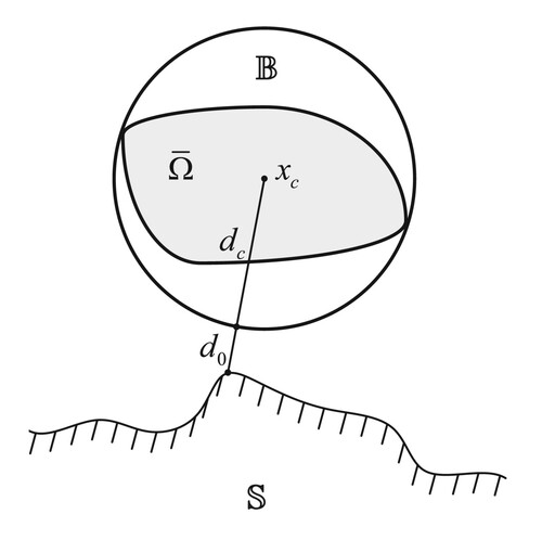
Firstly, let us recall the concept of singular points of sub-fully actuated systems, introduced in Duan (2021c). For simplicity, in this paper let us consider a simpler case and impose the following assumption.

Assumption A3

The matrix $B(\cdot )$ in system (1(1) $\begin{array}{rl}\left[\begin{array}{c}{x}_1^{\left({\mu }_1\right)}\\ x_2^{\left({\mu }_2\right)}\\ ⋮\\ x_{\eta }^{\left({\mu }_{\eta }\right)}\end{array}\right]& =\left[\begin{array}{c}{f}_1\left(x_k^{\left(0\sim {\mu }_k-1\right)}{|}_{k=1\sim \eta },\zeta ,t\right)\\ f_2\left(x_k^{\left(0\sim {\mu }_k-1\right)}{|}_{k=1\sim \eta },\zeta ,t\right)\\ ⋮\\ f_{\eta }\left(x_k^{\left(0\sim {\mu }_k-1\right)}{|}_{k=1\sim \eta },\zeta ,t\right)\end{array}\right]\\ & +B\left(x_k^{\left(0\sim {\mu }_k-1\right)}{|}_{k=1\sim \eta },\zeta ,t\right)u+\mathrm{\Gamma }d,\end{array}$(1) ) depends on only the state, that is, $B\left(\cdot \right)=B\left(x_k^{\left(0\sim {\mu }_k-1\right)}{|}_{k=1\sim \eta }\right).$

For the general case, please refer to Duan (2021c, 2021d).

6.1. Singularity and feasibility

For a sub-fully actuated system in the form of (1(1) $\begin{array}{rl}\left[\begin{array}{c}{x}_1^{\left({\mu }_1\right)}\\ x_2^{\left({\mu }_2\right)}\\ ⋮\\ x_{\eta }^{\left({\mu }_{\eta }\right)}\end{array}\right]& =\left[\begin{array}{c}{f}_1\left(x_k^{\left(0\sim {\mu }_k-1\right)}{|}_{k=1\sim \eta },\zeta ,t\right)\\ f_2\left(x_k^{\left(0\sim {\mu }_k-1\right)}{|}_{k=1\sim \eta },\zeta ,t\right)\\ ⋮\\ f_{\eta }\left(x_k^{\left(0\sim {\mu }_k-1\right)}{|}_{k=1\sim \eta },\zeta ,t\right)\end{array}\right]\\ & +B\left(x_k^{\left(0\sim {\mu }_k-1\right)}{|}_{k=1\sim \eta },\zeta ,t\right)u+\mathrm{\Gamma }d,\end{array}$(1) ) satisfying the above Assumption A3, the following concept is essential.

Definition 6.1

If $x_k^{(0\sim {\mu }_k-1)}\left(t\right){|}_{k=1\sim \eta }\in {\mathbb{R}}^{\varkappa }$ satisfies (83) $detB\left(x_k^{\left(0\sim {\mu }_k-1\right)}{|}_{k=1\sim \eta }\right)=0\text{or}\mathrm{\infty },$(83) then it is called a singular point of system (1(1) $\begin{array}{rl}\left[\begin{array}{c}{x}_1^{\left({\mu }_1\right)}\\ x_2^{\left({\mu }_2\right)}\\ ⋮\\ x_{\eta }^{\left({\mu }_{\eta }\right)}\end{array}\right]& =\left[\begin{array}{c}{f}_1\left(x_k^{\left(0\sim {\mu }_k-1\right)}{|}_{k=1\sim \eta },\zeta ,t\right)\\ f_2\left(x_k^{\left(0\sim {\mu }_k-1\right)}{|}_{k=1\sim \eta },\zeta ,t\right)\\ ⋮\\ f_{\eta }\left(x_k^{\left(0\sim {\mu }_k-1\right)}{|}_{k=1\sim \eta },\zeta ,t\right)\end{array}\right]\\ & +B\left(x_k^{\left(0\sim {\mu }_k-1\right)}{|}_{k=1\sim \eta },\zeta ,t\right)u+\mathrm{\Gamma }d,\end{array}$(1) ).

Let $\mathbb{S}$ be the set of all singular points of system (1(1) $\begin{array}{rl}\left[\begin{array}{c}{x}_1^{\left({\mu }_1\right)}\\ x_2^{\left({\mu }_2\right)}\\ ⋮\\ x_{\eta }^{\left({\mu }_{\eta }\right)}\end{array}\right]& =\left[\begin{array}{c}{f}_1\left(x_k^{\left(0\sim {\mu }_k-1\right)}{|}_{k=1\sim \eta },\zeta ,t\right)\\ f_2\left(x_k^{\left(0\sim {\mu }_k-1\right)}{|}_{k=1\sim \eta },\zeta ,t\right)\\ ⋮\\ f_{\eta }\left(x_k^{\left(0\sim {\mu }_k-1\right)}{|}_{k=1\sim \eta },\zeta ,t\right)\end{array}\right]\\ & +B\left(x_k^{\left(0\sim {\mu }_k-1\right)}{|}_{k=1\sim \eta },\zeta ,t\right)u+\mathrm{\Gamma }d,\end{array}$(1) ), that is, $\mathbb{S}=\left\{\left.x_k^{\left(0\sim {\mu }_k-1\right)}\left(t\right){|}_{k=1\sim \eta }\right|\text{Equation~(83) holds}\right\}.$Then the following set $\mathbb{F}={\mathbb{R}}^{\varkappa }\mathrm{\setminus }\mathbb{S},$is called the set of feasible points of system (1(1) $\begin{array}{rl}\left[\begin{array}{c}{x}_1^{\left({\mu }_1\right)}\\ x_2^{\left({\mu }_2\right)}\\ ⋮\\ x_{\eta }^{\left({\mu }_{\eta }\right)}\end{array}\right]& =\left[\begin{array}{c}{f}_1\left(x_k^{\left(0\sim {\mu }_k-1\right)}{|}_{k=1\sim \eta },\zeta ,t\right)\\ f_2\left(x_k^{\left(0\sim {\mu }_k-1\right)}{|}_{k=1\sim \eta },\zeta ,t\right)\\ ⋮\\ f_{\eta }\left(x_k^{\left(0\sim {\mu }_k-1\right)}{|}_{k=1\sim \eta },\zeta ,t\right)\end{array}\right]\\ & +B\left(x_k^{\left(0\sim {\mu }_k-1\right)}{|}_{k=1\sim \eta },\zeta ,t\right)u+\mathrm{\Gamma }d,\end{array}$(1) ). In general, the system (1(1) $\begin{array}{rl}\left[\begin{array}{c}{x}_1^{\left({\mu }_1\right)}\\ x_2^{\left({\mu }_2\right)}\\ ⋮\\ x_{\eta }^{\left({\mu }_{\eta }\right)}\end{array}\right]& =\left[\begin{array}{c}{f}_1\left(x_k^{\left(0\sim {\mu }_k-1\right)}{|}_{k=1\sim \eta },\zeta ,t\right)\\ f_2\left(x_k^{\left(0\sim {\mu }_k-1\right)}{|}_{k=1\sim \eta },\zeta ,t\right)\\ ⋮\\ f_{\eta }\left(x_k^{\left(0\sim {\mu }_k-1\right)}{|}_{k=1\sim \eta },\zeta ,t\right)\end{array}\right]\\ & +B\left(x_k^{\left(0\sim {\mu }_k-1\right)}{|}_{k=1\sim \eta },\zeta ,t\right)u+\mathrm{\Gamma }d,\end{array}$(1) ) is called a sub-fully actuated system if $\mathbb{F}$ is different from ${\mathbb{R}}^{\varkappa }$ and is a set with dimension not less than 1 (Duan, 2021c).

To implement the controllers (7(7) $\left\{\begin{array}{rl}u& =-B^{-1}\left(x_k^{\left(0\sim {\mu }_k-1\right)}{|}_{k=1\sim \eta },\zeta ,t\right)\\ & \times \left[f\left(x_k^{\left(0\sim {\mu }_k-1\right)}{|}_{k=1\sim \eta },\zeta ,t\right)-v\right]\\ v& =K_{PD}{x}_k^{\left(0\sim {\mu }_k-1\right)}{|}_{k=1\sim \eta }\\ & +K_I{\int }_0^t\left[y\left(\sigma \right)-y_{\mathrm{c}}\right]\mathrm{d}\sigma ,\end{array}\right.$(7) ), (43(43) $\left\{\begin{array}{rl}u& =-B^{-1}\left(x_k^{\left(0\sim {\mu }_k-1\right)}{|}_{k=1\sim \eta },\zeta ,t\right)\\ & \times \left[f\left(x_k^{\left(0\sim {\mu }_k-1\right)}{|}_{k=1\sim \eta },\zeta ,t\right)-v\right]\\ v& =K_{FB}{x}_k^{\left(0\sim {\mu }_k-1\right)}{|}_{k=1\sim \eta }+K_{FF}{x}_{\mathrm{m}},\end{array}\right.$(43) ) and (52(52) $\left\{\begin{array}{rl}u& =-B^{-1}\left(x_k^{\left(0\sim {\mu }_k-1\right)}{|}_{k=1\sim \eta },\zeta ,t\right)\\ & \times \left[f\left(x_k^{\left(0\sim {\mu }_k-1\right)}{|}_{k=1\sim \eta },\zeta ,t\right)-v\right]\\ v& =K_{PD}{x}_k^{\left(0\sim {\mu }_k-1\right)}{|}_{k=1\sim \eta }+K_{FF}{x}_{\mathrm{m}}\\ & +K_I{\int }_0^t\left[y\left(\sigma \right)-y_{\mathrm{m}}\left(\sigma \right)-y_{\mathrm{c}}\right]\mathrm{d}\sigma ,\end{array}\right.$(52) ), the following feasibility condition (84) $x_k^{\left(0\sim {\mu }_k-1\right)}{|}_{k=1\sim \eta }\notin \mathbb{S},$(84) or, equivalently, (85) $x_k^{\left(0\sim {\mu }_k-1\right)}{|}_{k=1\sim \eta }\in \mathbb{F},$(85) needs to be met. Such a problem can be generally turned into a state constrained control problem and solved via an eigenstructure-based approach.

6.2. State constrained control

It is easily observed that, with our designed PID and MRT controllers, the closed-loop systems are linear constant ones, and generally obey the form of (58(58) $\dot{x}=A_{\mathrm{c}}x+\mathrm{\Gamma }{u}_r,$(58) ).

The state constrained control problem can be simply stated as follows:

Problem 6.1

Let $[A,B]$ be stabilisable, and $\mathbb{F}\subset {\mathbb{R}}^n$ be a manifold. For the linear system (56(56) $\dot{x}=Ax+Bu+\mathrm{\Gamma }{u}_r,$(56) ) with $u_r$ being a constant external input, find a state feedback controller (57(57) $u=Kx,$(57) ) such that the following requirements are met:

1. the matrix $A_{\mathrm{c}}=A+BK$ is Hurwitz; and

2. the state constraint $x\in$ $\mathbb{F}$ is met.

In Duan (2021d), a solution to such a problem based on Lyapunov matrix equations is presented. In this section, let us present an eigenstructure-based solution to the problem.

Clearly, the equilibrium point of the system (58(58) $\dot{x}=A_{\mathrm{c}}x+\mathrm{\Gamma }{u}_r,$(58) ) is (86) $x_e=-A_{\mathrm{c}}^{-1}\mathrm{\Gamma }{u}_r.$(86) Let $z=x-x_e,$then the system (58(58) $\dot{x}=A_{\mathrm{c}}x+\mathrm{\Gamma }{u}_r,$(58) ) is transformed into (87) $\dot{z}=A_{\mathrm{c}}z.$(87) Applying Lemma 5.1 to system (56(56) $\dot{x}=Ax+Bu+\mathrm{\Gamma }{u}_r,$(56) ), gives the feedback gain (88) $\left\{\begin{array}{l}K=W{V}^{-1}\\ V=N_{0}Z+N_{1}ZF+\cdots +N_{\omega }Z{F}^{\omega }\\ W=D_{0}Z+D_{1}ZF+\cdots +D_{\omega }Z{F}^{\omega },\end{array}\right.$(88) and eventually, there holds (89) $A_{\mathrm{c}}=VF{V}^{-1}.$(89) For only demonstration, let us consider the case of (90) $F=\text{diag}\left(s_i,i=1,2,\dots ,n\right),$(90) where $s_i,i=1,2,\dots ,n$ are a series of negative real scalars. While the result can be easily generalised into the case that F contains a diagonal real block of the following form: $\left[\begin{array}{cc}\alpha & \text{β}\\ -\text{β}& \alpha \end{array}\right].$With F given by (90(90) $F=\text{diag}\left(s_i,i=1,2,\dots ,n\right),$(90) ), the solution to the closed-loop system (87(87) $\dot{z}=A_{\mathrm{c}}z.$(87) ) is given by $\begin{array}{rl}z\left(t\right)& =e^{A_{c}t}z\left(0\right)\\ & =V{e}^{Ft}{V}^{-1}z\left(0\right)\\ & =V\text{diag}\left(e^{s_{i}t},i=1,2,\dots ,n\right)V^{-1}z\left(0\right),\end{array}$which gives (91) $∥z\left(t\right)∥\le ∥V∥∥V^{-1}∥∥z\left(0\right)∥.$(91) Therefore, for some $d_0>0,$ $∥V∥∥V^{-1}∥∥z\left(0\right)∥<d_0,$implies $∥z\left(t\right)∥<d_0,t\ge 0.$The above process clearly proves the following important lemma about state constrained control.

Lemma 6.2

Let $[A,B]$ be stabilisable, $u_r$ be constant, $d_0$ be the maximum number such that (92) $\mathrm{\Omega }=\left\{\left.x\right|∥x-x_e∥<d_0\right\}\subset \mathbb{F},$(92) and K be the state feedback gain, of the state feedback controller (57(57) $u=Kx,$(57) ), given by (88(88) $\left\{\begin{array}{l}K=W{V}^{-1}\\ V=N_{0}Z+N_{1}ZF+\cdots +N_{\omega }Z{F}^{\omega }\\ W=D_{0}Z+D_{1}ZF+\cdots +D_{\omega }Z{F}^{\omega },\end{array}\right.$(88) ), with F being a stable diagonal matrix given by (90(90) $F=\text{diag}\left(s_i,i=1,2,\dots ,n\right),$(90) ). Further, if the initial values are chosen to satisfy (93) $\nu \left(V\right)∥x\left(0\right)-x_e∥<d_0,$(93) then (94) $x\left(t\right)\in \mathrm{\Omega }\subset \mathbb{F},\mathrm{\forall }t\ge 0.$(94)

Recalling (86(86) $x_e=-A_{\mathrm{c}}^{-1}\mathrm{\Gamma }{u}_r.$(86) ) and (89(89) $A_{\mathrm{c}}=VF{V}^{-1}.$(89) ), we have (95) $x_e=-V{F}^{-1}{V}^{-1}\mathrm{\Gamma }{u}_r,$(95) which is dependent on V. Furthermore, the condition (93(93) $\nu \left(V\right)∥x\left(0\right)-x_e∥<d_0,$(93) ) is also dependent on $\nu \left(V\right).$ In applications, it is desirable to select the free parameter matrix Z to let $d_0$ be as big as possible, and $\nu \left(V\right)$ be as small as possible.

6.3. Feasibility conditions

In this subsection, let us apply the above Lemma 6.2 to our generalised PID control and MRT control.

6.3.1. Case of PID control

The purpose here is to provide a solution to Problem 2.1 with the feasibility requirement (85(85) $x_k^{\left(0\sim {\mu }_k-1\right)}{|}_{k=1\sim \eta }\in \mathbb{F},$(85) ) satisfied. The general idea is as follows.

Applying Lemma 5.3, we can obtain a pair of polynomial matrices $\tilde{N}\left(s\right)$ and $\tilde{D}\left(s\right)$ in the form of (79(79) $\left\{\begin{array}{ll}\tilde{N}\left(s\right)=\sum _{i=0}^{\tilde{\omega }}{\tilde{N}}_i{s}^i,& {\tilde{N}}_i\in {\mathbb{R}}^{\left(\varkappa +m\right)\times r}\\ \tilde{D}\left(s\right)=\sum _{i=0}^{\tilde{\omega }}{\tilde{D}}_i{s}^i,& {\tilde{D}}_i\in {\mathbb{R}}^{r\times r}.\end{array}\right.$(79) ) satisfying the RCF (71(71) ${\left(sI-\tilde{A}\right)}^{-1}\tilde{B}=\tilde{N}\left(s\right){\tilde{D}}^{-1}\left(s\right)$(71) ). Then according to the second conclusion in Lemma 5.1, the general expression of the gain matrix $K=\left[K_{PD}{K}_I\right]$ can be obtained as in (80(80) $\left\{\begin{array}{l}\left[K_{PD}{K}_I\right]=\tilde{W}{\tilde{V}}^{-1}\\ \tilde{V}={\tilde{N}}_0\tilde{Z}+{\tilde{N}}_1\tilde{Z}\tilde{F}+\cdots +{\tilde{N}}_{\omega }\tilde{Z}{\tilde{F}}^{\tilde{\omega }}\\ \tilde{W}={\tilde{D}}_0\tilde{Z}+{\tilde{D}}_1\tilde{Z}\tilde{F}+\cdots +{\tilde{D}}_{\omega }\tilde{Z}{\tilde{F}}^{\tilde{\omega }},\end{array}\right.$(80) ). Finally, with the help of Lemma 6.2, the result about generalised PID control of sub-fully actuated systems can be obtained.

The equilibrium point of the closed-loop system is easily obtained as (96) $\left[\begin{array}{c}{X}_{\mathrm{e}}\\ q_{\mathrm{e}}\end{array}\right]=-{\tilde{A}}_{\mathrm{c}}^{-1}\left[\begin{array}{c}{B}_E\mathrm{\Gamma }d\\ -y_{\mathrm{c}}\end{array}\right]=-\tilde{V}{\tilde{F}}^{-1}{\tilde{V}}^{-1}\left[\begin{array}{c}{B}_E\mathrm{\Gamma }d\\ -y_{\mathrm{c}}\end{array}\right],$(96) where the disturbance d may be substituted by an estimate.

Theorem 6.3

Consider the system (2(2) $\begin{array}{rl}{x}_k^{\left({\mu }_k\right)}{|}_{k=1\sim \eta }& =f\left(x_k^{\left(0\sim {\mu }_k-1\right)}{|}_{k=1\sim \eta },\zeta ,t\right)\\ & +B\left(x_k^{\left(0\sim {\mu }_k-1\right)}{|}_{k=1\sim \eta },\zeta ,t\right)u+\mathrm{\Gamma }d,\end{array}$(2) ) with the output equation (5(5) $y=C{x}_k^{\left(0\sim {\mu }_k-1\right)}{|}_{k=1\sim \eta },$(5) ). Let Assumptions A2 and A3 and condition (21(21) $\text{rank}\left[\begin{array}{cc}{A}_E& B_E\\ C& 0\end{array}\right]=\varkappa +m.$(21) ) be met, and d be absent, $K=\left[K_{PD}{K}_I\right]$ be given by (80(80) $\left\{\begin{array}{l}\left[K_{PD}{K}_I\right]=\tilde{W}{\tilde{V}}^{-1}\\ \tilde{V}={\tilde{N}}_0\tilde{Z}+{\tilde{N}}_1\tilde{Z}\tilde{F}+\cdots +{\tilde{N}}_{\omega }\tilde{Z}{\tilde{F}}^{\tilde{\omega }}\\ \tilde{W}={\tilde{D}}_0\tilde{Z}+{\tilde{D}}_1\tilde{Z}\tilde{F}+\cdots +{\tilde{D}}_{\omega }\tilde{Z}{\tilde{F}}^{\tilde{\omega }},\end{array}\right.$(80) ), with $\tilde{F}\in {\mathbb{R}}^{(\varkappa +m)\times (\varkappa +m)}$ being chosen to be a stable diagonal matrix, and $\tilde{Z}\in {\mathbb{R}}^{r\times (\varkappa +m)}$ be an arbitrary parameter matrix satisfying the constraint (81(81) $det\left({\tilde{N}}_0\tilde{Z}+{\tilde{N}}_1\tilde{Z}\tilde{F}+\cdots +{\tilde{N}}_{\omega }\tilde{Z}{\tilde{F}}^{\tilde{\omega }}\right)\ne 0.$(81) ). Further, if the initial values are chosen to satisfy (97) $\nu \left(\tilde{V}\right)∥\left[\begin{array}{c}{x}_k^{\left(0\sim {\mu }_k-1\right)}{|}_{k=1\sim \eta }\left(0\right)\\ q\left(0\right)\end{array}\right]-\left[\begin{array}{c}{X}_{\mathrm{e}}\\ q_{\mathrm{e}}\end{array}\right]∥\le d_0,$(97) where $d_0$ is the maximum number such that (98) $\mathrm{\Omega }=\left\{z\mid z\in {\mathbb{R}}^{\varkappa },∥z-X_{\mathrm{e}}∥\le d_0\right\}\subset \mathbb{F},$(98) then the controller (7(7) $\left\{\begin{array}{rl}u& =-B^{-1}\left(x_k^{\left(0\sim {\mu }_k-1\right)}{|}_{k=1\sim \eta },\zeta ,t\right)\\ & \times \left[f\left(x_k^{\left(0\sim {\mu }_k-1\right)}{|}_{k=1\sim \eta },\zeta ,t\right)-v\right]\\ v& =K_{PD}{x}_k^{\left(0\sim {\mu }_k-1\right)}{|}_{k=1\sim \eta }\\ & +K_I{\int }_0^t\left[y\left(\sigma \right)-y_{\mathrm{c}}\right]\mathrm{d}\sigma ,\end{array}\right.$(7) ) for the system (2(2) $\begin{array}{rl}{x}_k^{\left({\mu }_k\right)}{|}_{k=1\sim \eta }& =f\left(x_k^{\left(0\sim {\mu }_k-1\right)}{|}_{k=1\sim \eta },\zeta ,t\right)\\ & +B\left(x_k^{\left(0\sim {\mu }_k-1\right)}{|}_{k=1\sim \eta },\zeta ,t\right)u+\mathrm{\Gamma }d,\end{array}$(2) ) guarantees (26(26) $\begin{array}{rl}\underset{t\to \mathrm{\infty }}{lim}y\left(t\right)& =y_{\mathrm{c}},\end{array}$(26) )–(28(28) $\underset{t\to \mathrm{\infty }}{lim}{x}_{1\sim \eta }\left(t\right)=-\mathring{C}{\tilde{A}}_c^{-1}\left[\begin{array}{c}{B}_E\mathrm{\Gamma }d\\ -y_{\mathrm{c}}\end{array}\right].$(28) ) and the feasibility requirement (85(85) $x_k^{\left(0\sim {\mu }_k-1\right)}{|}_{k=1\sim \eta }\in \mathbb{F},$(85) ).

Proof.

It follows from Lemma 6.2 that, under condition (97(97) $\nu \left(\tilde{V}\right)∥\left[\begin{array}{c}{x}_k^{\left(0\sim {\mu }_k-1\right)}{|}_{k=1\sim \eta }\left(0\right)\\ q\left(0\right)\end{array}\right]-\left[\begin{array}{c}{X}_{\mathrm{e}}\\ q_{\mathrm{e}}\end{array}\right]∥\le d_0,$(97) ), there also holds (99) $∥\left[\begin{array}{c}{x}_k^{\left(0\sim {\mu }_k-1\right)}{|}_{k=1\sim \eta }\left(t\right)\\ q\left(t\right)\end{array}\right]-\left[\begin{array}{c}{X}_{\mathrm{e}}\\ q_{\mathrm{e}}\end{array}\right]∥\le d_0,\mathrm{\forall }t\ge 0.$(99) Thus we have (100) $\begin{array}{rl}& ∥x_k^{\left(0\sim {\mu }_k-1\right)}{|}_{k=1\sim \eta }\left(t\right)-X_{\mathrm{e}}∥\\ & \le ∥\left[\begin{array}{c}{x}_k^{\left(0\sim {\mu }_k-1\right)}{|}_{k=1\sim \eta }\left(t\right)\\ q\left(t\right)\end{array}\right]-\left[\begin{array}{c}{X}_{\mathrm{e}}\\ q_{\mathrm{e}}\end{array}\right]∥\\ & \le d_0,\mathrm{\forall }t\ge 0.\end{array}$(100) This shows $x_k^{\left(0\sim {\mu }_k-1\right)}{|}_{k=1\sim \eta }\left(t\right)\in \mathrm{\Omega }\subset \mathbb{F}.$The proof is done.

6.3.2. Case of MRT control

For simplicity, let us only consider the MRT control scheme without an integration, that is, the case of Problem 5.2, but with Assumption A1 removed, and the additional feasibility requirement (85(85) $x_k^{\left(0\sim {\mu }_k-1\right)}{|}_{k=1\sim \eta }\in \mathbb{F},$(85) ) added. Again, the idea of solving this problem is to adopt the following outline:

Applying Lemma 5.2, gives a pair of polynomial matrices $N\left(s\right)$ and $D\left(s\right)$ in the form of (61(61) $\left\{\begin{array}{ll}N\left(s\right)=\sum _{i=0}^{\omega }{N}_i{s}^i,& N_i\in {\mathbb{R}}^{n\times r},\\ D\left(s\right)=\sum _{i=0}^{\omega }{D}_i{s}^i,& D_i\in {\mathbb{R}}^{r\times r}.\end{array}\right.$(61) ) satisfying the RCF (69(69) $\left\{\begin{array}{l}N\left(s\right)=\text{blockdiag}\left(N_k\left(s\right),k=1,2,\dots ,\eta \right)\\ D\left(s\right)=\text{blockdiag}\left(I_{r_k}{s}^{{\mu }_k},k=1,2,\dots ,\eta \right).\end{array}\right.$(69) ). Then according to the second conclusion in Lemma 5.1, the general expression of the gain matrix $K_{FB}$ can be obtained. Finally, with the help of Lemma 6.2, the feasibility condition for MRT in sub-fully actuated systems can be obtained.

Before implementing this idea, let us first impose some assumption on the reference model (9(9) $\left\{\begin{array}{l}{\dot{x}}_{\mathrm{m}}=A_{\mathrm{m}}{x}_{\mathrm{m}}\\ y_{\mathrm{m}}=C_{\mathrm{m}}{x}_{\mathrm{m}},\end{array}\right.$(9) ). Let ${\mathrm{\Omega }}_0\subset {\mathbb{R}}^p$ be a set of admissible initial values of system (9(9) $\left\{\begin{array}{l}{\dot{x}}_{\mathrm{m}}=A_{\mathrm{m}}{x}_{\mathrm{m}}\\ y_{\mathrm{m}}=C_{\mathrm{m}}{x}_{\mathrm{m}},\end{array}\right.$(9) ), then the following objective set can be defined: (101) $\mathrm{\Omega }=\left\{G{x}_{\mathrm{m}}\left(t\right)|{\dot{x}}_{\mathrm{m}}=A_{\mathrm{m}}{x}_{\mathrm{m}},t\ge 0,x_{\mathrm{m}}\left(0\right)\in {\mathrm{\Omega }}_0\right\}.$(101) Theoretically, the reference model (9(9) $\left\{\begin{array}{l}{\dot{x}}_{\mathrm{m}}=A_{\mathrm{m}}{x}_{\mathrm{m}}\\ y_{\mathrm{m}}=C_{\mathrm{m}}{x}_{\mathrm{m}},\end{array}\right.$(9) ) is allowed to be unstable. However, such a case is very rare. Thus in this subsection the reference model (9(9) $\left\{\begin{array}{l}{\dot{x}}_{\mathrm{m}}=A_{\mathrm{m}}{x}_{\mathrm{m}}\\ y_{\mathrm{m}}=C_{\mathrm{m}}{x}_{\mathrm{m}},\end{array}\right.$(9) ) is restricted to be stable or critically stable. As a consequence, the above set Ω defined in (101(101) $\mathrm{\Omega }=\left\{G{x}_{\mathrm{m}}\left(t\right)|{\dot{x}}_{\mathrm{m}}=A_{\mathrm{m}}{x}_{\mathrm{m}},t\ge 0,x_{\mathrm{m}}\left(0\right)\in {\mathrm{\Omega }}_0\right\}.$(101) ) is bounded. Furthermore, since the reference model is often ideally chosen, it is reasonable to require that Ω is far away enough from $\mathbb{S}$.

If $\overline{\mathrm{\Omega }}$ represents the closed-cover of Ω, and $d(\mathbb{B},\mathbb{S})$ represents the distance between the two sets $\mathbb{B}$ and $\mathbb{S}$, which is defined by $d\left(\mathbb{B},\mathbb{S}\right)=inf\left\{∥y-z∥|y\in \mathbb{B},z\in \mathbb{S}\right\},$then the above discussion motivates us to propose the following assumption.

Assumption A4

There exists a $x_c\in \overline{\mathrm{\Omega }}$ and a constant $d_c>0,$ such that (102) $\overline{\mathrm{\Omega }}\subset \mathbb{B}=\left\{x|∥x-x_c∥\le d_c\right\},$(102) and (103) $d_0=d\left(\mathbb{B},\mathbb{S}\right)>0.$(103)

Clearly, (102(102) $\overline{\mathrm{\Omega }}\subset \mathbb{B}=\left\{x|∥x-x_c∥\le d_c\right\},$(102) ) assumes the boundedness of set Ω, while (103(103) $d_0=d\left(\mathbb{B},\mathbb{S}\right)>0.$(103) ) assumes that Ω is far away enough from $\mathbb{S}$.

With the above preparation, the following result about the MRT control of the sub-fully actuated system (2(2) $\begin{array}{rl}{x}_k^{\left({\mu }_k\right)}{|}_{k=1\sim \eta }& =f\left(x_k^{\left(0\sim {\mu }_k-1\right)}{|}_{k=1\sim \eta },\zeta ,t\right)\\ & +B\left(x_k^{\left(0\sim {\mu }_k-1\right)}{|}_{k=1\sim \eta },\zeta ,t\right)u+\mathrm{\Gamma }d,\end{array}$(2) ) can be proven.

Theorem 6.4

Consider the system (2(2) $\begin{array}{rl}{x}_k^{\left({\mu }_k\right)}{|}_{k=1\sim \eta }& =f\left(x_k^{\left(0\sim {\mu }_k-1\right)}{|}_{k=1\sim \eta },\zeta ,t\right)\\ & +B\left(x_k^{\left(0\sim {\mu }_k-1\right)}{|}_{k=1\sim \eta },\zeta ,t\right)u+\mathrm{\Gamma }d,\end{array}$(2) ) with the output equation (5(5) $y=C{x}_k^{\left(0\sim {\mu }_k-1\right)}{|}_{k=1\sim \eta },$(5) ). Let Assumptions A2${}^{\mathrm{\prime }}$, A3 and A4 be met, and d = 0; $K_{FB}$ be given by (78(78) $\left\{\begin{array}{l}{K}_{FB}=W{V}^{-1}\\ V=N_{0}Z+N_{1}ZF+\cdots +N_{\omega }Z{F}^{\omega }\\ W=D_{0}Z+D_{1}ZF+\cdots +D_{\omega }Z{F}^{\omega },\end{array}\right.$(78) ), with $F\in {\mathbb{R}}^{\varkappa \times \varkappa }$ being chosen to be a stable diagonal matrix, and $Z\in {\mathbb{R}}^{r\times \varkappa }$ be an arbitrary parameter matrix satisfying the constraint (65(65) $det\left(N_{0}Z+N_{1}ZF+\cdots +N_{\omega }Z{F}^{\omega }\right)\ne 0.$(65) ). Further, if the initial values are chosen to satisfy $x_{\mathrm{m}}\left(0\right)\in {\mathrm{\Omega }}_0$ and (104) $\nu \left(V\right)∥x_k^{\left(0\sim {\mu }_k-1\right)}{|}_{k=1\sim \eta }\left(0\right)-G{x}_{\mathrm{m}}\left(0\right)∥\le d_0,$(104) where V is given by (78(78) $\left\{\begin{array}{l}{K}_{FB}=W{V}^{-1}\\ V=N_{0}Z+N_{1}ZF+\cdots +N_{\omega }Z{F}^{\omega }\\ W=D_{0}Z+D_{1}ZF+\cdots +D_{\omega }Z{F}^{\omega },\end{array}\right.$(78) ), then the controller (43(43) $\left\{\begin{array}{rl}u& =-B^{-1}\left(x_k^{\left(0\sim {\mu }_k-1\right)}{|}_{k=1\sim \eta },\zeta ,t\right)\\ & \times \left[f\left(x_k^{\left(0\sim {\mu }_k-1\right)}{|}_{k=1\sim \eta },\zeta ,t\right)-v\right]\\ v& =K_{FB}{x}_k^{\left(0\sim {\mu }_k-1\right)}{|}_{k=1\sim \eta }+K_{FF}{x}_{\mathrm{m}},\end{array}\right.$(43) ) for the system guarantees (44(44) $\underset{t\to \mathrm{\infty }}{lim}\left[y\left(t\right)-y_{\mathrm{m}}\left(t\right)\right]=0,$(44) )–(45(45) $\underset{t\to \mathrm{\infty }}{lim}\left[x_k^{\left(0\sim {\mu }_k-1\right)}{|}_{k=1\sim \eta }-G{x}_{\mathrm{m}}\right]=0.$(45) ) and the feasibility requirement (85(85) $x_k^{\left(0\sim {\mu }_k-1\right)}{|}_{k=1\sim \eta }\in \mathbb{F},$(85) ).

Proof.

Recall that, under given conditions, the controller (43(43) $\left\{\begin{array}{rl}u& =-B^{-1}\left(x_k^{\left(0\sim {\mu }_k-1\right)}{|}_{k=1\sim \eta },\zeta ,t\right)\\ & \times \left[f\left(x_k^{\left(0\sim {\mu }_k-1\right)}{|}_{k=1\sim \eta },\zeta ,t\right)-v\right]\\ v& =K_{FB}{x}_k^{\left(0\sim {\mu }_k-1\right)}{|}_{k=1\sim \eta }+K_{FF}{x}_{\mathrm{m}},\end{array}\right.$(43) ) results in the closed-loop system given by (40(40) $\left\{\begin{array}{l}\delta \dot{x}=A_E^c\delta x\\ \delta y=C\delta x,\end{array}\right.$(40) ), with $A_E^c=VF{V}^{-1}.$Applying Lemma 6.2, we have, due to (104(104) $\nu \left(V\right)∥x_k^{\left(0\sim {\mu }_k-1\right)}{|}_{k=1\sim \eta }\left(0\right)-G{x}_{\mathrm{m}}\left(0\right)∥\le d_0,$(104) ), the following relation: (105) $∥x_k^{\left(0\sim {\mu }_k-1\right)}{|}_{k=1\sim \eta }\left(t\right)-G{x}_{\mathrm{m}}\left(t\right)∥\le d_0,\mathrm{\forall }t\ge 0.$(105) On the other hand, since $x_{\mathrm{m}}\left(0\right)\in {\mathrm{\Omega }}_0,$ there holds $G{x}_{\mathrm{m}}\in \mathrm{\Omega }$. Further, recalling $\mathrm{\Omega }\subset \mathbb{B}$, we obviously have (106) $∥G{x}_{\mathrm{m}}-x_c∥\le d_c.$(106) Therefore, using (105(105) $∥x_k^{\left(0\sim {\mu }_k-1\right)}{|}_{k=1\sim \eta }\left(t\right)-G{x}_{\mathrm{m}}\left(t\right)∥\le d_0,\mathrm{\forall }t\ge 0.$(105) ) and (106(106) $∥G{x}_{\mathrm{m}}-x_c∥\le d_c.$(106) ), gives $\begin{array}{rl}& ∥x_k^{\left(0\sim {\mu }_k-1\right)}{|}_{k=1\sim \eta }\left(t\right)-x_c∥\\ & \le ∥x_k^{\left(0\sim {\mu }_k-1\right)}{|}_{k=1\sim \eta }\left(t\right)-G{x}_{\mathrm{m}}∥+∥G{x}_{\mathrm{m}}-x_c∥\\ & \le d_0+d_c,\mathrm{\forall }t\ge 0.\end{array}$This clearly implies (85(85) $x_k^{\left(0\sim {\mu }_k-1\right)}{|}_{k=1\sim \eta }\in \mathbb{F},$(85) ) (see Figure 1).

Figure 1. Geometric relation between Ω and $\mathbb{S}$.

Remark 6.1

It is easily recognised that the feasibility conditions given in Theorems 6.3 and 6.4 may be conservative. In certain cases, e.g. when $detB\left(x_k^{(0\sim {\mu }_k-1)}{|}_{k=1\sim \eta }\right)$ is dependent on only some, but not all, $x_k$'s and their derivatives, less conservative initial value ranges can be provided by applying decoupled design approaches (see Section 3.3, and also Duan (2021d)). The next section gives a demonstration of this idea with an illustrative example.

Remark 6.2

The results presented in this subsection are conservative but are strictly correct. While in many cases, the set of singular points is only a low-dimensional hyperplane in the space ${\mathbb{R}}^{\varkappa }$, in this case, as long as the steady response of the closed-loop system does not intersect with $\mathbb{S}$, the probability that the system response in the transient process intersects with $\mathbb{S}$ is very small. This is why some practical applications on control of sub-fully actuated systems simply overlook such a feasibility analysis problem. However, for applications of high-grade security or high cost, a trial and test approach is certainly not acceptable.

7. Illustrative example

7.1. The system model

The Example 6.2 in Duan (2021c) treats a classical example system proposed in Brocket (1983). In the treatment of Duan (2021c), the problem is reduced to the control of a HOFA system. When a disturbance d is added to the system, it appears as follows: (107) $\left[\begin{array}{c}\ddot{z}\\ \dot{x}\end{array}\right]=B\left(x,\dot{z}\right)u+\left[\begin{array}{c}1\\ 0\end{array}\right]d,$(107) where $B\left(x,\dot{z}\right)=\left[\begin{array}{cc}x& \frac{\dot{z}}{x}\\ 0& 1\end{array}\right],$and $u=\left[\begin{array}{c}{u}_1\\ u_2\end{array}\right]$is the control vector. Clearly, the set of singular points of the system is $\mathbb{S}=\left\{\left.\left[\begin{array}{c}z\\ \dot{z}\\ x\end{array}\right]\right|x=0\right\}.$In the Example 6.2 in Duan (2021c), a decoupled design is proposed, which gives a nonconservative feasibility condition. However, with decoupled designs, the design degrees of freedom is dramatically reduced. Now in this section, coupled designs using the PID and MRT control are presented.

By the following control transformation, (108) $u=B^{-1}\left(x,\dot{z}\right)v,$(108) where v is a two-dimensional intermediate control vector, the system is turned into (109) $\left[\begin{array}{c}\ddot{z}\\ \dot{x}\end{array}\right]=v.$(109) which can be converted into the following state-space form: (110) $\left[\begin{array}{c}{\dot{z}}^{\left(0\sim 1\right)}\\ \dot{x}\end{array}\right]=A_E\left[\begin{array}{c}{z}^{\left(0\sim 1\right)}\\ x\end{array}\right]+B_{E}v,$(110) where (111) $A_E=\left[\begin{array}{ccc}0& 1& 0\\ 0& 0& 0\\ 0& 0& 0\end{array}\right],B_E=\left[\begin{array}{cc}0& 0\\ 1& 0\\ 0& 1\end{array}\right].$(111) The output equation of the system is taken to be (112) $y=x=C\left[\begin{array}{c}{z}^{\left(0\sim 1\right)}\\ x\end{array}\right],$(112) where $C=\left[001\right].$

7.2. Generalised PID design

In this section, our aim of the design is to let the system output y regulate at a constant value $y_{\mathrm{c}}.$ As a result of Theorem 3.3, the controller finally designed for the system is (113) $\left\{\begin{array}{l}u=B^{-1}\left(x,\dot{z}\right)v\\ v=K_{PD}\left[\begin{array}{c}{z}^{\left(0\sim 1\right)}\\ x\end{array}\right]+K_I{\int }_0^t\left[y\left(\sigma \right)-y_{\mathrm{c}}\right]\mathrm{d}\sigma .\end{array}\right.$(113) It follows from Theorem 3.3 that $K=\left[K_{PD}{K}_I\right]$is determined by (114) ${\tilde{A}}_c=\tilde{A}+\tilde{B}K=\tilde{V}\tilde{F}{\tilde{V}}^{-1},$(114) where (115) $\begin{array}{rl}\tilde{A}& =\left[\begin{array}{cc}{A}_E& 0\\ C& 0\end{array}\right]=\left[\begin{array}{cccc}0& 1& 0& 0\\ 0& 0& 0& 0\\ 0& 0& 0& 0\\ 0& 0& 1& 0\end{array}\right],\end{array}$(115) (116) $\begin{array}{rl}\tilde{B}& =\left[\begin{array}{c}{B}_E\\ 0\end{array}\right]=\left[\begin{array}{cc}0& 0\\ 1& 0\\ 0& 1\\ 0& 0\end{array}\right],\end{array}$(116) and $\tilde{F}$ is a stable real matrix, and $\tilde{V}$ a nonsingular real matrix.

7.2.1. Solution of RCFs

It follows from Lemmas 5.2 and 5.3, (117) $\begin{array}{rl}& N_1\left(s\right)=\left[\begin{array}{c}1\\ s\end{array}\right],D_1\left(s\right)=s^2.\end{array}$(117) (118) $\begin{array}{rl}& N_2\left(s\right)=1,D_2\left(s\right)=s.\end{array}$(118) and (119) $N\left(s\right)=\left[\begin{array}{cc}1& 0\\ s& 0\\ 0& 1\end{array}\right],D\left(s\right)=\left[\begin{array}{cc}{s}^2& 0\\ 0& s\end{array}\right].$(119) Thus (120) $N_0=\left[\begin{array}{cc}1& 0\\ 0& 0\\ 0& 1\end{array}\right],N^{\mathrm{\#}}\left(s\right)=\left[\begin{array}{cc}0& 0\\ 1& 0\\ 0& 0\end{array}\right].$(120) Note that $C{N}_0=\left[01\right],$we have (121) $P=1,T_1=\left[\begin{array}{c}0\\ 1\end{array}\right],T_2=\left[\begin{array}{c}1\\ 0\end{array}\right].$(121) Thus it follows from Lemma 5.3 that (122) $\tilde{N}\left(s\right)=\left[\begin{array}{cc}1& 0\\ s& 0\\ 0& s\\ 0& 1\end{array}\right],\tilde{D}\left(s\right)=\left[\begin{array}{cc}{s}^2& 0\\ 0& s^2\end{array}\right],$(122) which gives $\begin{array}{rl}{\tilde{N}}_0& =\left[\begin{array}{cc}1& 0\\ 0& 0\\ 0& 0\\ 0& 1\end{array}\right],{\tilde{N}}_1=\left[\begin{array}{cc}0& 0\\ 1& 0\\ 0& 1\\ 0& 0\end{array}\right],\\ {\tilde{D}}_0& ={\tilde{D}}_1=0,{\tilde{D}}_2=I_2.\end{array}$

7.2.2. Solution of $K_{PD}$ and $K_I$

Choose $\tilde{F}=\text{diag}\left(-1,-2,-3,-4\right),$we obtain (123) $\left\{\begin{array}{l}\tilde{V}={\tilde{N}}_0\tilde{Z}+{\tilde{N}}_1\tilde{Z}\tilde{F}\\ \tilde{W}=\tilde{Z}{\tilde{F}}^2.\end{array}\right.$(123) By minimising the condition number $\nu \left(\tilde{V}\right)=∥\tilde{V}∥∥{\tilde{V}}^{-1}∥,$the parameter matrix $\tilde{Z}$ is obtained as (124) $\begin{array}{rl}\tilde{Z}& =\left[\begin{array}{cc}-107.4746& -42.8741\\ -12.3083& 18.5433\end{array}\right.\\ & \left.\begin{array}{cc}-110.4591& 170.2421\\ -151.2066& -57.0688\end{array}\right],\end{array}$(124) which corresponds to $\nu \left(\tilde{V}\right)=\mathrm{9.1778.}$ Hence $\begin{array}{rl}K& =\tilde{W}{\tilde{V}}^{-1}\\ & =\left[\begin{array}{cccc}-7.9952& -5.9984& 0.0868& 0.2947\\ 0.1093& 0.0478& -4.0016& -3.0058\end{array}\right].\end{array}$Thus (125) $\begin{array}{rl}{K}_{PD}& =\left[\begin{array}{ccc}-7.9952& -5.9984& 0.0868\\ 0.1093& 0.0478& -4.0016\end{array}\right],\end{array}$(125) (126) $\begin{array}{rl}{K}_I& =\left[\begin{array}{c}0.2947\\ -3.0058\end{array}\right].\end{array}$(126) It can be obtained that ${\tilde{A}}_c=\left[\begin{array}{cccc}0& 1& 0& 0\\ -7.9952& -5.9984& 0.0868& 0.2947\\ 0.1093& 0.0478& -4.0016& -3.0058\\ 0& 0& 1& 0\end{array}\right].$Further choose (127) $y_{\mathrm{c}}=16,$(127) we have (128) $\left[\begin{array}{c}{X}_{\mathrm{e}}\\ q_{\mathrm{e}}\end{array}\right]=-{\tilde{A}}_c^{-1}\left[\begin{array}{c}0\\ -y_{\mathrm{c}}\end{array}\right]=\left[\begin{array}{c}-0.6121\\ 0\\ 16.0000\\ -21.3225\end{array}\right].$(128) Note that the distance of $y_{\mathrm{c}}$ from $\mathbb{S}$ is $d_0=y_{\mathrm{c}}=16,$ by (97(97) $\nu \left(\tilde{V}\right)∥\left[\begin{array}{c}{x}_k^{\left(0\sim {\mu }_k-1\right)}{|}_{k=1\sim \eta }\left(0\right)\\ q\left(0\right)\end{array}\right]-\left[\begin{array}{c}{X}_{\mathrm{e}}\\ q_{\mathrm{e}}\end{array}\right]∥\le d_0,$(97) ) the set of feasible initial values is obtained as (129) $\begin{array}{rl}& ∥\left[\begin{array}{c}{x}_k^{\left(0\sim {\mu }_k-1\right)}{|}_{k=1\sim \eta }\left(0\right)\\ q\left(0\right)\end{array}\right]-\left[\begin{array}{c}{X}_{\mathrm{e}}\\ q_{\mathrm{e}}\end{array}\right]∥\\ & \le \frac{d_0}{\nu \left(\tilde{V}\right)}=\mathrm{1.74334.}\end{array}$(129)

7.3. Model reference tracking design

Let the coefficient matrices of the reference model (9(9) $\left\{\begin{array}{l}{\dot{x}}_{\mathrm{m}}=A_{\mathrm{m}}{x}_{\mathrm{m}}\\ y_{\mathrm{m}}=C_{\mathrm{m}}{x}_{\mathrm{m}},\end{array}\right.$(9) ) be taken as $A_{\mathrm{m}}=\left[\begin{array}{cc}0& 1\\ -4& 0\end{array}\right],C_{\mathrm{m}}=\left[10\right].$It can be easily observed that this corresponds to (130) $y_{\mathrm{m}}\left(t\right)=\rho \sin \left(2t+\varphi \right),$(130) where ρ and ϕ are two real numbers determined by the initial values of the reference model.

In view of (119(119) $N\left(s\right)=\left[\begin{array}{cc}1& 0\\ s& 0\\ 0& 1\end{array}\right],D\left(s\right)=\left[\begin{array}{cc}{s}^2& 0\\ 0& s\end{array}\right].$(119) ), we have (131) $\begin{array}{rl}{N}_0& =\left[\begin{array}{cc}1& 0\\ 0& 0\\ 0& 1\end{array}\right],N_1=\left[\begin{array}{cc}0& 0\\ 1& 0\\ 0& 0\end{array}\right],\end{array}$(131) (132) $\begin{array}{rl}{D}_0& =0,D_1=\left[\begin{array}{cc}0& 0\\ 0& 1\end{array}\right],D_2=\left[\begin{array}{cc}1& 0\\ 0& 0\end{array}\right],\end{array}$(132) thus Assumption A2${}^{\mathrm{\prime }}$, that is, (133) $C{N}_{0}Z+C{N}_{1}Z{A}_{\mathrm{m}}=C_{\mathrm{m}},$(133) gives (134) $Z=\left[\begin{array}{cc}\alpha & \text{β}\\ 1& 0\end{array}\right],$(134) where α and β are two arbitrary real scalars. Therefore, it follows from (75(75) $\left\{\begin{array}{l}G=N_{0}Z+N_{1}Z{A}_{\mathrm{m}}+\cdots +N_{\omega }Z{A}_{\mathrm{m}}^{\omega }\\ H=D_{0}Z+D_{1}Z{A}_{\mathrm{m}}+\cdots +D_{\omega }Z{A}_{\mathrm{m}}^{\omega },\end{array}\right.$(75) ) and (134(134) $Z=\left[\begin{array}{cc}\alpha & \text{β}\\ 1& 0\end{array}\right],$(134) ) that (135) $\begin{array}{rl}G& =N_{0}Z+N_{1}Z{A}_{\mathrm{m}}=\left[\begin{array}{cc}\alpha & \text{β}\\ -4\text{β}& \alpha \\ 1& 0\end{array}\right],\end{array}$(135) (136) $\begin{array}{rl}H& =D_{1}Z{A}_{\mathrm{m}}+D_{2}Z{A}_m^2=\left[\begin{array}{cc}-4\alpha & -4\text{β}\\ 0& 1\end{array}\right].\end{array}$(136) For simplicity, let us just take $K_{PD}$ and $K_I$ as in (125(125) $\begin{array}{rl}{K}_{PD}& =\left[\begin{array}{ccc}-7.9952& -5.9984& 0.0868\\ 0.1093& 0.0478& -4.0016\end{array}\right],\end{array}$(125) ) and (126(126) $\begin{array}{rl}{K}_I& =\left[\begin{array}{c}0.2947\\ -3.0058\end{array}\right].\end{array}$(126) ), respectively, then $K_{FF}$ is given by (42(42) $K_{FF}=H-K_{FB}G.$(42) ). Through minimising $J=∥H\left(\alpha ,\text{β}\right)-K_{PD}G\left(\alpha ,\text{β}\right)∥,$the optimal parameters are derived as $\alpha =-0.7845,\text{β}=\mathrm{0.0702.}$Hence $K_{FF}=\left[\begin{array}{cc}-4.9050& -4.4257\\ 4.1008& 1.0298\end{array}\right].$

7.4. Simulation results

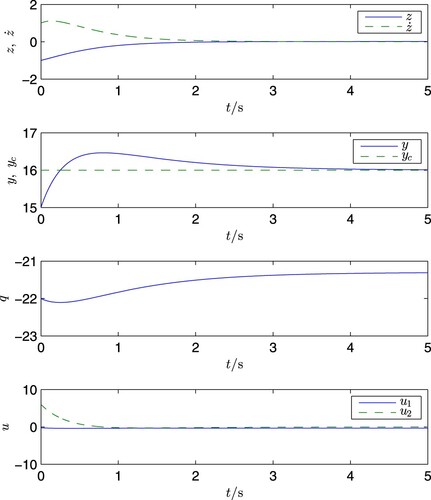
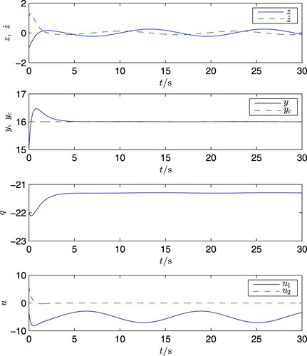
7.4.1. PID control

When the initial values are chosen as (137) $\begin{array}{rl}z\left(0\right)& =-1,\dot{z}\left(0\right)=1,x\left(0\right)=15,\\ q\left(0\right)& =-22,\end{array}$(137) it can be easily verified that the condition (129(129) $\begin{array}{rl}& ∥\left[\begin{array}{c}{x}_k^{\left(0\sim {\mu }_k-1\right)}{|}_{k=1\sim \eta }\left(0\right)\\ q\left(0\right)\end{array}\right]-\left[\begin{array}{c}{X}_{\mathrm{e}}\\ q_{\mathrm{e}}\end{array}\right]∥\\ & \le \frac{d_0}{\nu \left(\tilde{V}\right)}=\mathrm{1.74334.}\end{array}$(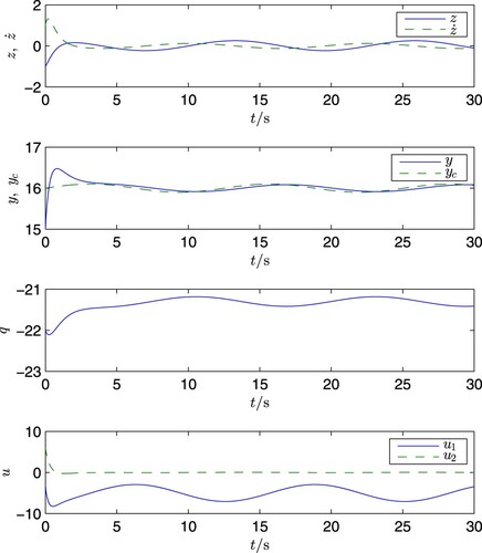129) ) is met. Corresponding to the cases of d = 0 and $d=5.0,$ the corresponding simulation results are shown in Figures 2 and 3, respectively. It is clearly seen from these figures that in both cases the signal $y\left(t\right)$ remains the same and tracks $y_{\mathrm{c}},$ the results clearly support the theoretical conclusions.

Figure 2. Generalised PID control, d = 0.0.

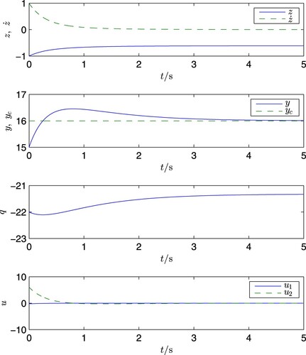
Figure 3. Generalised PID control, d = 5.0.

7.4.2. Model reference tracking

Again, take $y_{\mathrm{c}}=16,$ and the system initial values as in (137(137) $\begin{array}{rl}z\left(0\right)& =-1,\dot{z}\left(0\right)=1,x\left(0\right)=15,\\ q\left(0\right)& =-22,\end{array}$(137) ). Furthermore, take the initial value of the reference model as $x_{\mathrm{m}}\left(0\right)=\left[\begin{array}{c}5\\ 0\end{array}\right].$Then, for the case of d = 0 and $d=5.0,$ the simulation is also carried out, and the results are shown in Figures 4 and 5, respectively. It is clearly seen from these two figures that in both cases $y\left(t\right)$ and $y_{\mathrm{m}}\left(t\right)$ remain unaltered and $y_{\mathrm{m}}\left(t\right)-y\left(t\right)$ gets closed to $y_{\mathrm{c}}=16.$ Again, the results coincide with the theories.

Figure 4. Model reference control, d = 0.0.

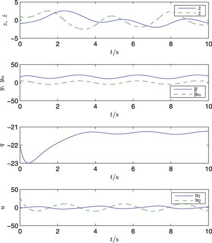
Figure 5. Model reference control, d = 5.0.

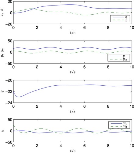
7.4.3. Case of slow time-varying d and $y_{\mathrm{c}}$

In this subsection, let us further check the effect of the designed controllers when applied to systems with slow time-varying disturbance d and a slow time-varying commend signal $y_{\mathrm{c}}$. For paper length limitation, here only the results of the generalised PID controller are presented.

Case A: $d\left(t\right)$ is time-varying only

Consider the case where only the disturbance d is replaced with the following time-varying signal (138) $d\left(t\right)=5+2\cos \left(0.5t\right),$(138) while keeping all the other parameters unchanged. The simulation results are shown in Figure 6. Comparison of Figure 6 with Figure 3 gives the following observation: the time-varying disturbance does affect the variables z and $\dot{z},$ but it almost has no affection on the steady response of the variable y, as desired.

Figure 6. Generalised PID control, Case A.

Case B: Both d and $y_{\mathrm{c}}$ are time-varying

In the case that d is replaced with that in (138(138) $d\left(t\right)=5+2\cos \left(0.5t\right),$(138) ), and, simultaneously, $y_{\mathrm{c}}$ is replaced with $y_{\mathrm{c}}\left(t\right)=16+0.1\sin \left(0.5t\right),$while keeping the initial values still the same as in (137(137) $\begin{array}{rl}z\left(0\right)& =-1,\dot{z}\left(0\right)=1,x\left(0\right)=15,\\ q\left(0\right)& =-22,\end{array}$(137) ), the simulation results are shown in Figure 7. It is observed that in this case the variable $y\left(t\right)$ still follows the signal $y_{\mathrm{c}}\left(t\right)$ closely, as desired.

Figure 7. Generalised PID control, Case B.

8. Conclusions

Tracking and regulation is one of the most important design objectives in control systems design. For tracking and regulation in linear systems, the problem has been well solved. While for nonlinear systems, with the widely used state-space approaches the problem is only solved for some very special systems and the results are also often limited to certain local senses.

Parallel to the state-space approaches, HOFA approaches have been recently proposed and demonstrated to be much more effective in dealing with system control problems (Duan, 2020a, 2020b, 2020c, 2021a, 2021b, 2021c, 2021e, 2021f, 2021g, 2021h). It is further shown in this paper that, once a general nonlinear dynamical system is represented by a HOFA model, the problem of tracking control can be solved perfectly in the sense that the closed-loop system becomes constant linear, besides realisation of the required asymptotical tracking property. Concretely, the paper has shown the following:

1. the well-known PID scheme can be easily generalised to suit a HOFA system subject to a constant or slow time-varying disturbance, and to achieve asymptotical tracking of a constant or slow time-varying signal;

2. an MRT controller also exists for an HOFA system, which guarantees asymptotical tracking of the signal generated by the reference model, and the tracking error remains unchanged when the system is subject to a constant disturbance;

3. the closed-loop systems resulted in by both designs are constant linear, and the controllers as well as the closed-loop systems can be completely parameterised, with the degrees of freedom properly utilised to further improve the system performance; and

4. both designs can be generalised to the case of sub-fully actuated systems, and effective feasibility conditions in terms of the system initial values are provided by using the parameterised closed-loop eigenstructure.

Acknowledgements

The author is grateful to his Ph.D. students Qin Zhao, Guangtai Tian, Xiubo Wang, Weizhen Liu, Kaixin Cui, etc., for helping him with reference selection and proofreading. His particular thanks go to his student Tianyi Zhao for help with the simulations.

Disclosure statement

No potential conflict of interest was reported by the author(s).

Additional information

Funding

This work has been partially supported by the Major Program of National Natural Science Foundation of China [grant numbers 61690210, 61690212], the National Natural Science Foundation of China [grant number 61333003] and the Self-Planned Task of State Key Laboratory of Robotics and System (HIT) [grant number SKLRS201716A].

Notes on contributors

Guangren Duan

Guangren Duan received his Ph.D. degree in Control Systems Sciences from Harbin Institute of Technology, Harbin, P. R. China, in 1989. After a two-year post-doctoral experience at the same university, he became professor of control systems theory at that university in 1991. He is the founder and now the Honourary Director of the Center for Control Theory and Guidance Technology at Harbin Institute of Technology, and recently he is also in charge of the Center for Control Science and Technology at the Sounthen University of Science and Technology. He visited the University of Hull, the University of Sheffield, and also the Queen's University of Belfast, UK, from December 1996 to October 2002, and has served as Member of the Science and Technology Committee of the Chinese Ministry of Education, Vice President of the Control Theory and Applications Committee, Chinese Association of Automation (CAA), and Associate Editors of a few international journals. He is currently an Academician of the Chinese Academy of Sciences, and Fellow of CAA, IEEE and IET. His main research interests include parametric control systems design, nonlinear systems, descriptor systems, spacecraft control and magnetic bearing control. He is the author and co-author of 5 books and over 340 SCI indexed publications.

Appendix. Proof of Lemma 5.3

Since $[A_E,B_E]$ is controllable, there exists a unimodular matrix $Q\left(s\right)=\left[\begin{array}{cc}\ast & N\left(s\right)\\ \ast & D\left(s\right)\end{array}\right],$which satisfies $\left[s{I}_{\varkappa }-A_E{B}_E\right]Q\left(s\right)=\left[I_{\varkappa }0\right].$Using the above relation, yields $\begin{array}{rl}& \text{rank}\left[s{I}_{\varkappa +m}-\tilde{A}\tilde{B}\right]\\ & =\text{rank}\left[\begin{array}{ccc}s{I}_{\varkappa }-A_E& 0& B_E\\ -C& s{I}_m& 0\end{array}\right]\\ & =\text{rank}\left[\begin{array}{ccc}s{I}_{\varkappa }-A_E& B_E& 0\\ -C& 0& s{I}_m\end{array}\right]\\ & =\text{rank}\left(\left[\begin{array}{ccc}s{I}_{\varkappa }-A_E& B_E& 0\\ -C& 0& s{I}_m\end{array}\right]\left[\begin{array}{cc}Q\left(s\right)& 0\\ 0& I_m\end{array}\right]\right)\\ & =\text{rank}\left[\begin{array}{ccc}{I}_{\varkappa }& 0& 0\\ \ast & -CN\left(s\right)& s{I}_m\end{array}\right]\\ & =\text{rank}\left[\begin{array}{ccc}{I}_{\varkappa }& 0& 0\\ 0& -C{N}_0& s{I}_m\end{array}\right]\\ & =\varkappa +\text{rank}C{N}_0,\mathrm{\forall }s\in \mathbb{C}.\end{array}$Therefore, $\text{rank}\left[s{I}_{\varkappa +m}-\tilde{A}\tilde{B}\right]=\varkappa +m,\mathrm{\forall }s\in \mathbb{C},$if and only if $\text{rank }C{N}_0=m,\mathrm{\forall }s\in \mathbb{C}.$Thus the first conclusion of the lemma follows from the well-known PBH criterion.

From (73(73) $PC{N}_0\left[T_1{T}_2\right]=\left[I_{m}0\right].$(73) ), it can be obtained that (A1) $\begin{array}{rl}PC{N}_0{T}_1& =I_m,\end{array}$(A1) (A2) $\begin{array}{rl}PC{N}_0{T}_2& =0.\end{array}$(A2) While the former is easily seen to be equivalent to (A3) $C{N}_0{T}_{1}P=I_m.$(A3) Using the above equations and the given conditions in the lemma, produces $\begin{array}{rl}& \left(sI-\tilde{A}\right)\left[\begin{array}{c}N\left(s\right)\\ C{N}^{\mathrm{\#}}\left(s\right)\end{array}\right]T_2-\tilde{B}D\left(s\right)T_2\\ & =\left(\left[\begin{array}{cc}sI-A_E& 0\\ -C& sI\end{array}\right]\left[\begin{array}{c}N\left(s\right)\\ C{N}^{\mathrm{\#}}\left(s\right)\end{array}\right]-\left[\begin{array}{c}{B}_E\\ 0\end{array}\right]D\left(s\right)\right)T_2\\ & =\left[\begin{array}{c}\left(sI-A_E\right)N\left(s\right)-B_{E}D\left(s\right)\\ -C{N}_0\end{array}\right]T_2\\ & =\left[\begin{array}{c}0\\ -C{N}_0{T}_2\end{array}\right]\\ & =0,\end{array}$and $\begin{array}{rl}& \left(sI-\tilde{A}\right)\left[\begin{array}{c}sN\left(s\right)\\ CN\left(s\right)\end{array}\right]T_{1}P-s\tilde{B}D\left(s\right)T_{1}P\\ & =\left(\left[\begin{array}{cc}sI-A_E& 0\\ -C& sI\end{array}\right]\left[\begin{array}{c}sN\left(s\right)\\ CN\left(s\right)\end{array}\right]-\left[\begin{array}{c}s{B}_{E}D\left(s\right)\\ 0\end{array}\right]\right)T_{1}P\\ & =s\left[\begin{array}{c}\left(sI-A_E\right)N\left(s\right)-B_{E}D\left(s\right)\\ 0\end{array}\right]T_{1}P\\ & =0.\end{array}$

Combining the above two aspects, proves that $\tilde{N}\left(s\right)$ and $\tilde{D}\left(s\right)$ satisfy the right factorisation (71(71) ${\left(sI-\tilde{A}\right)}^{-1}\tilde{B}=\tilde{N}\left(s\right){\tilde{D}}^{-1}\left(s\right)$(71) ).

Next, using a series of row transformations, finally gives $\begin{array}{rl}& \text{rank}\left[\begin{array}{c}\tilde{N}\left(s\right)\\ \tilde{D}\left(s\right)\end{array}\right]\\ & =\text{rank}\left[\begin{array}{cc}\left[\begin{array}{c}N\left(s\right)\\ C{N}^{\mathrm{\#}}\left(s\right)\\ D\left(s\right)\end{array}\right]T_2& \left[\begin{array}{c}sN\left(s\right)\\ CN\left(s\right)\\ sD\left(s\right)\end{array}\right]T_{1}P\end{array}\right]\\ & =\text{rank}\left[\begin{array}{cc}\left[\begin{array}{c}N\left(s\right)\\ D\left(s\right)\\ C{N}^{\mathrm{\#}}\left(s\right)\end{array}\right]T_2& \left[\begin{array}{c}sN\left(s\right)\\ sD\left(s\right)\\ CN\left(s\right)\end{array}\right]T_{1}P\end{array}\right]\\ & =\text{rank}\left[\begin{array}{cc}\left[\begin{array}{c}0\\ I_m\\ C{N}^{\mathrm{\#}}\left(s\right)\end{array}\right]T_2& \left[\begin{array}{c}0\\ s{I}_m\\ CN\left(s\right)\end{array}\right]T_{1}P\end{array}\right]\\ & =\text{rank}\left[\begin{array}{cc}\left[\begin{array}{c}0\\ I_m\\ 0\end{array}\right]T_2& \left[\begin{array}{c}0\\ s{I}_m\\ C{N}_0\end{array}\right]T_{1}P\end{array}\right]\\ & =\text{rank}\left[\begin{array}{cc}\left[\begin{array}{c}0\\ T_2\\ 0\end{array}\right]& \left[\begin{array}{c}0\\ s{T}_{1}P\\ I_m\end{array}\right]\end{array}\right]\end{array}$ $\begin{array}{rl}& =m+\left(r-m\right)\\ & =r,\end{array}$thus the right coprimeness of $\tilde{N}\left(s\right)$ and $\tilde{D}\left(s\right)$ is also preserved. The whole proof is then completed.

References

- Abdullah, A., & Zribi, M. (2009). Model reference control of LPV systems. Journal of the Franklin Institute, 346(9), 854–871. https://doi.org/10.1016/j.jfranklin.2009.04.006
- Ang, K. H., Chong, G., & Li, Y. (2005). PID control system analysis, design, and technology. IEEE Transactions on Control Systems Technology, 13(4), 559–576. https://doi.org/10.1109/TCST.2005.847331
- Åström, K. J., & Hägglund, T. (1995). PID controllers: Theory, design, and tuning. Instrument society of America.
- Åström, K. J., Hägglund, T., & Astrom, K. J. (2006). Advanced PID control. ISA-The Instrumentation, Systems, and Automation Society.
- Borase, R. P., Maghade, D. K., Sondkar, S. Y., & Pawar, S. N. (2020). A review of PID control, tuning methods and applications. International Journal of Dynamics and Control, 9, 818–827. https://doi.org/10.1007/s40435-020-00665-4
- Brocket, R. W. (1983). Asymptotic stability and feedback stabilisation. In Differential geometric control theory (pp. 112–121). Birkhauser.
- Chang, W. D., Hwang, R. C., & Hsieh, J. G. (2002). A self-tuning PID control for a class of nonlinear systems based on the Lyapunov approach. Journal of Process Control, 12(2), 233–242. https://doi.org/10.1016/S0959-1524(01)00041-5
- Cunha, J. P. V. S., Hsu, L., Costa, R. R., & Lizarralde, F. (2003). Output-feedback model-reference sliding mode control of uncertain multivariable systems. IEEE Transactions on Automatic Control, 48(12), 2245–2250. https://doi.org/10.1109/TAC.2003.820156
- Duan, G. R. (1992). Simple algorithm for robust pole assignment in linear output feedback. IEE Proceedings-Control Theory and Applications, 139(5), 465–470. https://doi.org/10.1049/ip-d.1992.0058
- Duan, G. R. (1993). Robust eigenstructure assignment via dynamical compensators. Automatica, 29(2), 469–474. https://doi.org/10.1016/0005-1098(93)90140-O
- Duan, G. R. (2015). Generalized Sylvester equations: Unified parametric solutions. CRC Press.
- Duan, G. R. (2016). Linear system theory (Vol. II, 3rd ed.). The Science Press.
- Duan, G. R. (2020a). High-order system approaches: I. Full-actuation and parametric design. Acta Automatica Sinica, 46(7), 1333–1345. (in Chinese). https://doi.org/10.16383/j.aas.c200234
- Duan, G. R. (2020b). High-order system approaches: II. Controllability and fully-actuation. Acta Automatica Sinica, 46(8), 1571–1581. (in Chinese). https://doi.org/10.1080/00207721.2020.1829168
- Duan, G. R. (2020c). High-order system approaches: III. Observability and observer design. Acta Automatica Sinica, 46(9), 1885–1895. (in Chinese). https://doi.org/10.16383/j.aas.c200370
- Duan, G. R. (2021a). High-order fully actuated system approaches: Part V. Robust adaptive control. International Journal of System Sciences, 52(10), 2129–2143. https://doi.org/10.1080/00207721.2021.1879964
- Duan, G. R. (2021b). High-order fully actuated system approaches: Part VI. Disturbance attenuation and decoupling. International Journal of System Sciences, 52(10), 2161–2181. https://doi.org/10.1080/00207721.2021.1879966
- Duan, G. R. (2021c). High-order fully actuated system approaches: Part VII. Controllability, stabilizability and parametric designs. International Journal of System Sciences. https://doi.org/10.1080/00207721.2021.1921307
- Duan, G. R. (2021d). High-order fully actuated system approaches: Part VIII. Optimal control with application in spacecraft attitude stabilization. International Journal of System Sciences. https://doi.org/10.1080/00207721.2021.1937750
- Duan, G. R. (2021e). High-order fully actuated system approaches: Part I. Models and basic procedure. International Journal of System Sciences, 52(2), 422–435. https://doi.org/10.16383/j.aas.c200234
- Duan, G. R. (2021f). High-order fully actuated system approaches: Part II. Generalized strict-feedback systems. International Journal of System Sciences, 52(3), 437–454. https://doi.org/10.1080/00207721.2020.1829168
- Duan, G. R. (2021g). High-order fully actuated system approaches: Part III. Robust control and high-order backstepping. International Journal of System Sciences, 52(5), 952–971. https://doi.org/10.1080/00207721.2020.1849863
- Duan, G. R. (2021h). High-order fully actuated system approaches: Part IV. Adaptive control and high-order backstepping. International Journal of System Sciences, 52(5), 972–989. https://doi.org/10.1080/00207721.2020.1849864
- Duan, G. R., & Huang, L. (2008). Robust model following control for a class of second-order dynamical systems subject to parameter uncertainties. Transactions of the Institute of Measurement and Control, 30(2), 115–142. https://doi.org/10.1177/0142331207078510
- Duan, G. R., Liu, W. Q., & Liu, G. P. (2001). Robust model reference control for multivariable linear systems subject to parameter uncertainties. Proceedings of the Institution of Mechanical Engineers, Part I: Journal of Systems and Control Engineering, 215(6), 599–610. https://doi.org/10.1243/0959651011541337
- Duan, G. R., & Zhang, B. (2007). Robust model-reference control for descriptor linear systems subject to parameter uncertainties. Journal of Control Theory and Applications, 5(3), 213–220. https://doi.org/10.1007/s11768-006-6025-z
- Gonçalves, E. N., Bachur, W. E. G., Palhares, R. M., & Takahashi, R. H. C. (2011). Robust H2/ H∞ reference model dynamic output-feedback control synthesis. International Journal of Control, 84(12), 2067–2080. https://doi.org/10.1080/00207179.2011.633232
- Ho, M. T., & Lin, C. Y. (2003). PID controller design for robust performance. IEEE Transactions on Automatic Control, 48(8), 1404–1409. https://doi.org/10.1109/TAC.2003.815028
- Pathak, K. B., & Adhyaru, D. M. (2012). Survey of model reference adaptive control. In 2012 Nirma university international conference on engineering (pp. 1–6).
- Shekhar, A., & Sharma, A. (2018). Review of model reference adaptive control. In 2018 International conference on information, communication, engineering and technology (pp. 29–31).
- Silva, G. J., Datta, A., & Bhattacharyya, S. P. (2002). New results on the synthesis of PID controllers. IEEE Transactions on Automatic Control, 47(2), 241–252. https://doi.org/10.1109/9.983352
- Sun, J., Olbrot, A. W., & Polis, M. P. (1994). Robust stabilization and robust performance using model reference control and modeling error compensation. IEEE Transactions on Automatic Control, 39(3), 630–635. https://doi.org/10.1109/9.280776
- Yan, L., Hsu, L., Costa, R. R., & Lizarralde, F. (2008). A variable structure model reference robust control without a prior knowledge of high frequency gain sign. Automatica, 44(4), 1036–1044. https://doi.org/10.1016/j.automatica.2007.08.011
- Young, K. K. (1978). Design of variable structure model-following control systems. IEEE Transactions on Automatic Control, 23(6), 1079–1085. https://doi.org/10.1109/TAC.1978.1101913
- Zhang, J., & Guo, L. (2019). Theory and design of PID controller for nonlinear uncertain systems. IEEE Control Systems Letters, 3(3), 643–648. https://doi.org/10.1109/LCSYS.7782633
- Zhao, C., & Guo, L. (2017). PID controller design for second order nonlinear uncertain systems. Science China Information Sciences, 60(2), 1–13. https://doi.org/10.1007/s11432-016-0879-3
- Zhao, C., & Guo, L. (2020). Control of nonlinear uncertain systems by extended PID. IEEE Transactions on Automatic Control, 66(8), 3840–3847. https://doi.org/10.1109/TAC.2020.3030876
- Ziegler, J. G., & Nichols, N. B. (1942). Optimum settings for automatic controllers. Transactions of the A.S.M.E, 64(11), 759–765. https://doi.org/10.1115/1.2899060
- Ziegler, J. G., & Nichols, N. B. (1943). Process lags in automatic control circuits. Transactions of the A.S.M.E, 65(5), 433–443.