Decentralised output tracking of interconnected systems with unknown interconnections using sliding mode control

Abstract

In this paper, a class of nonlinear interconnected systems with matched and unmatched uncertainties is considered. The isolated subsystem dynamics are described by linear systems with nonlinear components. The matched uncertainties and unmatched unknown interconnection terms are assumed to be bounded by known nonlinear functions. Based on sliding mode techniques, a state feedback decentralised control scheme is proposed such that the outputs of the controlled interconnected system track given desired signals uniformly ultimately. The desired reference signals are allowed to be time-varying. Using appropriate transformations, the considered system is transformed into a new interconnected system with an appropriate structure to facilitate the sliding surface design and the decentralised control design. A set of conditions is proposed to guarantee that the designed controller drives the tracking errors onto the sliding surface. The sliding motion exhibited by the error dynamics is uniformly ultimately bounded. The developed results are applied to a river quality control problem. Simulation results show that the proposed decentralised control strategy is effective and feasible.

Keywords:

• Decentralised control
• large-scale system
• sliding mode control
• tracking control

1. Introduction

With the development of modern society, the need to control complicated systems is greatly increasing. This has motivated more researchers to focus on advanced control technology in order to deal with complex systems. Large-scale interconnected systems with non-linearities and uncertainties are typically complex systems. Such a class of systems widely exists in our real life, for example, a coupled inverted pendulum, river quality control, high-speed transportation and flight control (see, e.g. Lunze, 2020; Wu et al., 1998; Yan et al., 2017). Thus, these systems have received great attention and many results have been obtained (see, e.g. Onyeka et al., 2020; Su et al., 2018).

Large-scale systems are often mathematically modelled by interconnections of a set of lower-dimensional subsystems. One of the characteristics of such systems is that the dynamic of each subsystem is usually affected by the others due to the presence of the interconnections (Yan et al., 2017). It should be noted that large-scale systems are usually distributed in space widely. Thus the designed systems should have a high tolerance of data loss during data transfer due to possible broken/unknown interconnections as well as poor communications to guarantee that the controlled large-scale systems exhibit the required degree of robustness. The control problem for large-scale interconnected systems is challenging. Compared with the centralised control and distributed control, decentralised control needs local information only, and thus information or data transfer between subsystems is not required. Specifically, when the network linking different subsystems is broken, or the data transfer between subsystems is poor or unstable, a centralised control or distributed control scheme cannot be implemented because both centralised control and distributed control need the other subsystems' information. In such cases, decentralised control provides advantages over centralised control and is a popular choice in the control of large-scale interconnected systems (Yan et al., 2017).

Recently, the study of large-scale systems with interconnected terms has made great progress, and many interesting results have been obtained. In Kim et al. (2017), a large-scale fuzzy system with unknown interconnections is considered where matched uncertainties or disturbances are not included. There are also some results for interconnected systems (see, e.g. Huerta et al., 2019; Liu et al., 2019; Rinaldi et al., 2019; Song et al., 2020; Zhao et al., 2017), which require that interconnections are matched while unmatched interconnections and/or uncertainties are not involved. Moreover, some large-scale systems are considered to a simple or ideal dynamic model (see e.g. Han & Yan, 2020; Tan, 2020; Wan & Yin, 2020; Wu et al., 2018). These works just focus on a kind of special system structure that lacks generality. Decentralised sliding mode control has been developed in Yan et al. (2004) where the considered system is fully nonlinear with a more general structure, but only a stabilisation problem is considered where tracking control is not addressed.

Trajectory tracking and output tracking are important topics in both control theory and control engineering. Some tracking control results have been obtained by Cai and Hu (2017), Liu et al. (2019), and Zhao et al. (2017). However, most considered systems have special structures (see Han & Yan, 2020; Li & Liu, 2018; Tan, 2020; Wu et al., 2018). Decentralised tracking control for large-scale systems is considered in Pagilla et al. (2007), where model reference control is investigated. Tracking control for interconnected systems is considered based on adaptive fuzzy techniques in Ren et al. (2020). It should be noted that in both (Pagilla et al., 2007; Ren et al., 2020), it is required that the isolated subsystems are linear.

Sliding mode control is very popular in dealing with complex systems with uncertainties due to its unique characteristics (Song et al., 2022; Yan et al., 2014, 2020; Yao et al., 2020). On the one hand, the sliding mode dynamics are often composed of a reduced-order system when compared with the original system (Edwards & Spurgeon, 1998; Yan et al., 2017), which may simplify the corresponding system analysis and design. On the other hand, sliding mode control is totally robust to matched uncertainty and disturbances. This has resulted in the sliding mode control method being widely applied to deal with tracking problems, and many results have been achieved. Trajectory tracking control schemes based on sliding mode techniques are proposed for specific vehicles in Wei et al. (2020) and Zhao et al. (2021). An output tracking sliding mode control is designed in Ruiz-Duarte and Loukianov (2020), where the considered system is linear. Although tracking control for nonlinear systems with uncertainties is considered in Farzad and Mohammad Hossein (2018), where event-triggered tracking is considered, only matched disturbances are considered. In Zhu et al. (2020), a tracking problem for a class of large-scale systems with interconnections is considered using sliding mode control. However, it is required that the reference signals are constant. It should be emphasised that the results concerning output tracking for large-scale nonlinear interconnected systems with unknown interconnections are very few, specifically when the ideal reference signals are time-varying.

In this paper, a class of nonlinear interconnected systems is considered where both unknown matched uncertainty and unmatched nonlinear interconnections are considered. Suitable coordinate transformations are introduced to transform the nominal subsystems of the interconnected system to systems with special structure. This separates each subsystem of the transformed system into two parts to facilitate the system analysis and control design for output tracking. Then the tracking error dynamic systems are developed, and the sliding surface based on the tracking error system is designed. A set of conditions is proposed to guarantee the uniform ultimate boundedness of the corresponding sliding motion. A decentralised sliding mode control scheme is proposed to drive the nonlinear interconnected systems to the designed sliding surface. The main contributions of this paper can be summarised as follows

• The proposed control scheme is decentralised.

• The nominal subsystem of the interconnected systems is nonlinear, and the interconnections are unknown and unmatched.

• The developed results can guarantee that the system states are uniformly ultimately bounded while all the uncertainties and interconnections are bounded.

• The developed results have high robustness against uncertainties and unknown interconnections. Both the bounds on uncertainties and the unknown interconnections have more general nonlinear forms.

Finally, the obtained results are applied to a river quality control problem to show the practicability and feasibility of the proposed approach.

2. Preliminaries

In this paper, for a square matrix A, ${\lambda }_{min}\left(A\right)$ denotes the minimum eigenvalue of matrix A. The expression A>0 means that A is symmetric positive definite, and $I_n$ denotes the unit matrix with dimension of n. The set of $n\times m$ matrices with elements defined in R will be denoted by $R^{n\times m}$ and diag$\{A_1,A_2,\dots ,A_N\}$ represents a block-diagonal matrix with diagonal elements $A_1,A_2,\dots ,A_N$. $col(\cdot )$ is a column matrix. Finally, $\parallel \cdot \parallel$ denotes the Euclidean norm or its induced norm.

Consider initially a linear system (1) $\begin{array}{rl}& \dot{x}=Ax+Bu\\ & y=Cx\end{array}$(1) where $x\in R^n,u\in R^m$ and $y\in R^p$ are the states, inputs and outputs, respectively. The triple $(A,B,C)$ are constant matrices of appropriate dimensions with B being of full column rank and C being of full row rank.

Consider system (1(1) $\begin{array}{rl}& \dot{x}=Ax+Bu\\ & y=Cx\end{array}$(1) ) in the case of m = p, which means the system (1(1) $\begin{array}{rl}& \dot{x}=Ax+Bu\\ & y=Cx\end{array}$(1) ) is a square system. Since B has full column rank, there exists a coordinate transformation $\overline{x}=\overline{T}x$ such that in the new coordinate $\overline{x}$, the triple $(A,B,C)$ can be described by (2) $\overline{A}=\left[\begin{array}{cc}{A}_{11}& A_{12}\\ A_{21}& A_{22}\end{array}\right],\overline{B}=\left[\begin{array}{c}0\\ B_2\end{array}\right],\overline{C}=\left[\begin{array}{cc}{C}_1& C_2\end{array}\right]$(2) where $A_{11}\in R^{(n-m)\times (n-m)}$, $B_2\in R^{m\times m}$ is nonsingular. $C_1\in R^{m\times (n-m)}$.

Assume that rank$\left(CB\right)=m$ and the invariant zeros of $(A,B,C)$ lie in the left half plane. From Section 5.3 in Edwards and Spurgeon (1998), it follows that the matrix $C_2\in R^{m\times m}$ in (2(2) $\overline{A}=\left[\begin{array}{cc}{A}_{11}& A_{12}\\ A_{21}& A_{22}\end{array}\right],\overline{B}=\left[\begin{array}{c}0\\ B_2\end{array}\right],\overline{C}=\left[\begin{array}{cc}{C}_1& C_2\end{array}\right]$(2) ) is nonsingular because $m=\text{rank}\left(CB\right)=\text{rank}\left(\overline{C}\overline{B}\right)=\text{rank}\left(C_2{B}_2\right)$ and $B_2$ is nonsingular. Then, a coordinate transformation $\hat{x}=\hat{T}\overline{x}$ with $\hat{T}$ defined by (3) $\hat{T}=\left[\begin{array}{cc}I& 0\\ C_1& C_2\end{array}\right]$(3) is further introduced. Again from section 5.3 in Edwards and Spurgeon (1998), the triple $(\overline{A},\overline{B},\overline{C})$ in the new coordinates $\hat{x}$ has the following structure (4) $\hat{A}=\left[\begin{array}{cc}{\hat{A}}_{11}& {\hat{A}}_{12}\\ {\hat{A}}_{21}& {\hat{A}}_{22}\end{array}\right],\hat{B}=\left[\begin{array}{c}0\\ {\hat{B}}_2\end{array}\right],\hat{C}=\left[\begin{array}{cc}0& I\end{array}\right]$(4) where ${\hat{A}}_{11}\in R^{(n-m)\times (n-m)}$ is Hurwitz stable, ${\hat{B}}_2=C_2{B}_2$ is nonsingular.

Remark 2.1

It should be pointed out that the first transformation matrix $\overline{T}$ is used to change the original system $(A,B,C)$ into the regular form as in (2(2) $\overline{A}=\left[\begin{array}{cc}{A}_{11}& A_{12}\\ A_{21}& A_{22}\end{array}\right],\overline{B}=\left[\begin{array}{c}0\\ B_2\end{array}\right],\overline{C}=\left[\begin{array}{cc}{C}_1& C_2\end{array}\right]$(2) ), and the second transformation matrix $\hat{T}$ is to make that the sub-matrix ${\hat{A}}_{11}$ of the triple in (4(4) $\hat{A}=\left[\begin{array}{cc}{\hat{A}}_{11}& {\hat{A}}_{12}\\ {\hat{A}}_{21}& {\hat{A}}_{22}\end{array}\right],\hat{B}=\left[\begin{array}{c}0\\ {\hat{B}}_2\end{array}\right],\hat{C}=\left[\begin{array}{cc}0& I\end{array}\right]$(4) ) is Hurwitz stable and the matrix $\hat{C}$ in (4(4) $\hat{A}=\left[\begin{array}{cc}{\hat{A}}_{11}& {\hat{A}}_{12}\\ {\hat{A}}_{21}& {\hat{A}}_{22}\end{array}\right],\hat{B}=\left[\begin{array}{c}0\\ {\hat{B}}_2\end{array}\right],\hat{C}=\left[\begin{array}{cc}0& I\end{array}\right]$(4) ) has the form of $\left[0I\right]$.

3. System description and basic assumptions

Consider a nonlinear large-scale system formed by N interconnected subsystems as follows (5) $\begin{array}{rl}& {\dot{x}}_i=A_i{x}_i+f_i\left(x_i\right)+B_i(u_i+\mathrm{\Delta }{g}_i(x_i\left)\right)+h_i\left(x\right)\\ & y_i=C_i{x}_{i}i=1,2,\dots ,N\end{array}$(5) where $x=col(x_1,x_2,\dots ,x_N)$, $x_i\in R^{n_i}$, $u_i\in R^{m_i}$ and $y_i\in R^{m_i}$ represent the states, inputs and outputs of the ith subsystem respectively and $m_i<n_i$. The triple ($A_i,B_i,C_i$) represents constant matrices of appropriate dimensions where $B_i$ is full column rank and $C_i$ is full row rank. The function $f_i\left(x_i\right)$ represents a known nonlinear term in the ith subsystem which is used to model the nonlinear part of the ith isolated subsystem, and the matched uncertainty of the ith isolated subsystem is denoted by $\mathrm{\Delta }{g}_i\left(x_i\right)$ which is acting in the input channel. The term $h_i\left(x\right)$ represents the system interconnection, including all unmatched uncertainties. All the nonlinear functions in (5(5) $\begin{array}{rl}& {\dot{x}}_i=A_i{x}_i+f_i\left(x_i\right)+B_i(u_i+\mathrm{\Delta }{g}_i(x_i\left)\right)+h_i\left(x\right)\\ & y_i=C_i{x}_{i}i=1,2,\dots ,N\end{array}$(5) ) are assumed to be continuous in their arguments to guarantee the existence of solutions of the controlled system (5(5) $\begin{array}{rl}& {\dot{x}}_i=A_i{x}_i+f_i\left(x_i\right)+B_i(u_i+\mathrm{\Delta }{g}_i(x_i\left)\right)+h_i\left(x\right)\\ & y_i=C_i{x}_{i}i=1,2,\dots ,N\end{array}$(5) ).

The objective of this paper is, for a given desired signal $y_{id}\left(t\right)$, to design a decentralised sliding mode control such that the system output $y_i\left(t\right)$ of the controlled system (5(5) $\begin{array}{rl}& {\dot{x}}_i=A_i{x}_i+f_i\left(x_i\right)+B_i(u_i+\mathrm{\Delta }{g}_i(x_i\left)\right)+h_i\left(x\right)\\ & y_i=C_i{x}_{i}i=1,2,\dots ,N\end{array}$(5) ) can track the desired signal $y_{id}\left(t\right)$, i.e. the tracking errors $y_i\left(t\right)-y_{id}\left(t\right)$ are uniformly ultimately bounded for $i=1,2,\dots ,N$ while all the state variables of system (5(5) $\begin{array}{rl}& {\dot{x}}_i=A_i{x}_i+f_i\left(x_i\right)+B_i(u_i+\mathrm{\Delta }{g}_i(x_i\left)\right)+h_i\left(x\right)\\ & y_i=C_i{x}_{i}i=1,2,\dots ,N\end{array}$(5) ) are bounded.

Remark 3.1

It should be noted that in this paper, it is required that system (5(5) $\begin{array}{rl}& {\dot{x}}_i=A_i{x}_i+f_i\left(x_i\right)+B_i(u_i+\mathrm{\Delta }{g}_i(x_i\left)\right)+h_i\left(x\right)\\ & y_i=C_i{x}_{i}i=1,2,\dots ,N\end{array}$(5) ) is square for simplification of statement, that is, the dimension of each subsystem output is equal to the dimension of the corresponding subsystem input. However, the developed results can be easily extended to the case when the dimension of subsystem output is greater than the dimension of the subsystem input by slight modification.

In order to deal with the tracking problem stated above, some assumptions are imposed on the considered interconnected system (5(5) $\begin{array}{rl}& {\dot{x}}_i=A_i{x}_i+f_i\left(x_i\right)+B_i(u_i+\mathrm{\Delta }{g}_i(x_i\left)\right)+h_i\left(x\right)\\ & y_i=C_i{x}_{i}i=1,2,\dots ,N\end{array}$(5) ).

Assumption 3.1

All the invariant zeros of the triple $(A_i,B_i,C_i)$ lie in the left half plane, and rank$\left(C_i{B}_i\right)=m_i$ for $i=1,2,\dots ,N$.

It follows from the preliminaries in Section 2. Under Assumption 3.1, there exists a nonsingular coordinate transformation $z_i=T_i{x}_i$ such that the triple $({\hat{A}}_i,{\hat{B}}_i,{\hat{C}}_i)$ with respect to the new coordinates $z_i$ has the following structure (6) $\left[\begin{array}{cc}{\hat{A}}_{i11}& {\hat{A}}_{i12}\\ {\hat{A}}_{i21}& {\hat{A}}_{i22}\end{array}\right],\left[\begin{array}{c}0\\ {\hat{B}}_{i2}\end{array}\right],\left[\begin{array}{cc}0& I_{i2}\end{array}\right]$(6) where ${\hat{A}}_{i11}\in R^{(n_i-m_i)\times (n_i-m_i)}$ is Hurwitz stable, the square matrices ${\hat{B}}_{i2}\in R^{m_i\times m_i}$ and $I_{i2}\in R^{m_i\times m_i}$ are nonsingular for $i=1,2,\dots ,N$.

Assumption 3.2

Suppose that $f_i\left(x_i\right)$ has the decomposition $f_i\left(x_i\right)={\mathrm{\Gamma }}_i\left(x_i\right)x_i$, where ${\mathrm{\Gamma }}_i\in R^{n_i\times n_i}$ is a continuous function matrix for $i=1,2,\dots ,N$.

Remark 3.2

If $f_i\left(0\right)=0$ and $f_i$ is sufficiently smooth, then the decomposition $f_i\left(x_i\right)={\mathrm{\Gamma }}_i\left(x_i\right)x_i$ is guaranteed. Therefore, the limitation to $f_i\left(x_i\right)$ in Assumption 3.2 is not strict.

Assumption 3.3

There exist known continuous functions ${\rho }_i\left(x_i\right)$ and ${\eta }_i\left(x\right)$ with ${\eta }_i\left(0\right)=0$, and ${\eta }_i(\cdot )$ is differentiable at the origin, such that $\parallel \mathrm{\Delta }{g}_i\left(x_i\right)\parallel \le {\rho }_i\left(x_i\right)$ and $\parallel h_i\left(x\right)\parallel \le {\eta }_i(\Vert x\Vert )$ for $i=1,2,\dots ,N$.

Remark 3.3

If the interconnection $h_i\left(x\right)$ in (5(5) $\begin{array}{rl}& {\dot{x}}_i=A_i{x}_i+f_i\left(x_i\right)+B_i(u_i+\mathrm{\Delta }{g}_i(x_i\left)\right)+h_i\left(x\right)\\ & y_i=C_i{x}_{i}i=1,2,\dots ,N\end{array}$(5) ) satisfies the condition in Assumption 3.3, then from Yan et al. (1999) and Yan et al. (1998), it follows that there exist a continuous function ${\gamma }_i(\cdot )$ such that (7) ${\eta }_i(\Vert x\Vert )={\gamma }_i(\Vert x\Vert )\Vert x\Vert .$(7)

Remark 3.4

Assumption 3.3 requires that the bounds on all uncertainties in system (5(5) $\begin{array}{rl}& {\dot{x}}_i=A_i{x}_i+f_i\left(x_i\right)+B_i(u_i+\mathrm{\Delta }{g}_i(x_i\left)\right)+h_i\left(x\right)\\ & y_i=C_i{x}_{i}i=1,2,\dots ,N\end{array}$(5) ) are known but they are allowed to be nonlinear. Moreover, the unknown interconnections are allowed to have a more general nonlinear form.

Assumption 3.4

The desired output signal $y_{id}\left(t\right)$ is differentiable and satisfies

1. $\parallel y_{id}\left(t\right)\parallel \le L_{i1}$;

2. $\parallel \dot{\phantom{a}}{y}_{id}\left(t\right)\parallel \le L_{i2}$

for $t\in [0,\mathrm{\infty })$, where $L_{i1}$ and $L_{i2}$ are known constants for $i=1,2,\dots ,N$.

Remark 3.5

Assumption 3.4 is a limitation on the desired output signals $y_{id}\left(t\right)$. It is required that the desired output signal $y_{id}\left(t\right)$ and its derivative ${\dot{y}}_{id}\left(t\right)$ are bounded. This assumption is quite standard and can be satisfied in most practical cases.

4. System structure analysis

Consider the nonlinear interconnected system in (5(5) $\begin{array}{rl}& {\dot{x}}_i=A_i{x}_i+f_i\left(x_i\right)+B_i(u_i+\mathrm{\Delta }{g}_i(x_i\left)\right)+h_i\left(x\right)\\ & y_i=C_i{x}_{i}i=1,2,\dots ,N\end{array}$(5) ). Under Assumption 3.1 and from (6(6) $\left[\begin{array}{cc}{\hat{A}}_{i11}& {\hat{A}}_{i12}\\ {\hat{A}}_{i21}& {\hat{A}}_{i22}\end{array}\right],\left[\begin{array}{c}0\\ {\hat{B}}_{i2}\end{array}\right],\left[\begin{array}{cc}0& I_{i2}\end{array}\right]$(6) ), there exists a nonsingular coordinate transformation $z_i=T_i{x}_i$ such that in the new coordinate $z=col(z_1,z_2,\dots ,z_N)$, system (5(5) $\begin{array}{rl}& {\dot{x}}_i=A_i{x}_i+f_i\left(x_i\right)+B_i(u_i+\mathrm{\Delta }{g}_i(x_i\left)\right)+h_i\left(x\right)\\ & y_i=C_i{x}_{i}i=1,2,\dots ,N\end{array}$(5) ) has the following form (8) $\begin{array}{rl}{\dot{z}}_i& =\left[\begin{array}{cc}{\hat{A}}_{i11}& {\hat{A}}_{i12}\\ {\hat{A}}_{i21}& {\hat{A}}_{i22}\end{array}\right]z_i+\left[\begin{array}{c}{F}_{i1}\left(z_i\right)\\ F_{i2}\left(z_i\right)\end{array}\right]\\ & +\left[\begin{array}{c}0\\ {\hat{B}}_{i2}\end{array}\right](u_i+\mathrm{\Delta }{g}_i\left(T_i^{-1}{z}_i\right))+\left[\begin{array}{c}{H}_{i1}\left(z\right)\\ H_{i2}\left(z\right)\end{array}\right]\\ y_i& =\left[\begin{array}{cc}0& I_{i2}\end{array}\right]z_i,i=1,2,\dots ,N\end{array}$(8) where ${\hat{A}}_{i11}$ is stable, the square sub-matrices ${\hat{B}}_{i2}\in R^{m_i\times m_i}$ are nonsingular. $I_{i2}\in R^{m_i\times m_i}$ is an identity matrix, $col(F_{i1},F_{i2})=T_i{f}_i\left(x_i\right){|}_{x_i=T_i^{-1}{z}_i}$ and $F_{i1}\left(z_i\right)\in R^{n_i-m_i}$, $F_{i2}\left(z_i\right)\in R^{m_i}$. $col\left(H_{i1}\right(z),H_{i2}(z\left)\right)=T_i{h}_i\left(x\right){|}_{x=T^{-1}z}$ and $H_{i1}\left(z\right)\in R^{n_i-m_i}$, $H_{i2}\left(z\right)\in R^{m_i}$. The coordinate transformation $T:=col(T_1,T_2,\dots ,T_N)$.

Since ${\hat{A}}_{i11}$ is stable for $i=1,2,\dots ,N$, for any $Q_i>0$, the following Lyapunov equation has a unique solution $P_i>0$ (9) ${\hat{A}}_{i11}^{\mathsf{T}}{P}_i+P_i{\hat{A}}_{i11}=-Q_i,i=1,2,\dots ,N.$(9) Now, in order to fully exploit the structural characteristics, partition $z_i=col(z_{i1},z_{i2})$ with $z_{i1}\in R^{n_i-m_i}$ and $z_{i2}\in R^{m_i}$. It follows that (8(8) $\begin{array}{rl}{\dot{z}}_i& =\left[\begin{array}{cc}{\hat{A}}_{i11}& {\hat{A}}_{i12}\\ {\hat{A}}_{i21}& {\hat{A}}_{i22}\end{array}\right]z_i+\left[\begin{array}{c}{F}_{i1}\left(z_i\right)\\ F_{i2}\left(z_i\right)\end{array}\right]\\ & +\left[\begin{array}{c}0\\ {\hat{B}}_{i2}\end{array}\right](u_i+\mathrm{\Delta }{g}_i\left(T_i^{-1}{z}_i\right))+\left[\begin{array}{c}{H}_{i1}\left(z\right)\\ H_{i2}\left(z\right)\end{array}\right]\\ y_i& =\left[\begin{array}{cc}0& I_{i2}\end{array}\right]z_i,i=1,2,\dots ,N\end{array}$(8) ) can be described by (10) $\begin{array}{rl}{\dot{z}}_{i1}& ={\hat{A}}_{i11}{z}_{i1}+{\hat{A}}_{i12}{y}_i+F_{i1}(z_{i1},y_i)\\ & +H_{i1}(z_{11},y_1,\dots ,z_{N1},y_N)\end{array}$(10) (11) $\begin{array}{rl}{\dot{y}}_i& ={\hat{A}}_{i21}{z}_{i1}+{\hat{A}}_{i22}{y}_i+F_{i2}(z_{i1},y_i)\\ & +{\hat{B}}_{i2}(u_i+\mathrm{\Delta }{g}_i\left(T_i^{-1}{z}_i\right))\\ & +H_{i2}(z_{11},y_1,\dots ,z_{N1},y_N).\end{array}$(11) From system (8(8) $\begin{array}{rl}{\dot{z}}_i& =\left[\begin{array}{cc}{\hat{A}}_{i11}& {\hat{A}}_{i12}\\ {\hat{A}}_{i21}& {\hat{A}}_{i22}\end{array}\right]z_i+\left[\begin{array}{c}{F}_{i1}\left(z_i\right)\\ F_{i2}\left(z_i\right)\end{array}\right]\\ & +\left[\begin{array}{c}0\\ {\hat{B}}_{i2}\end{array}\right](u_i+\mathrm{\Delta }{g}_i\left(T_i^{-1}{z}_i\right))+\left[\begin{array}{c}{H}_{i1}\left(z\right)\\ H_{i2}\left(z\right)\end{array}\right]\\ y_i& =\left[\begin{array}{cc}0& I_{i2}\end{array}\right]z_i,i=1,2,\dots ,N\end{array}$(8) ) and Assumption 3.2, (12) $col(F_{i1},F_{i2})=T_i{\mathrm{\Gamma }}_i\left(x_i\right){|}_{x_i=T_i^{-1}{z}_i}{T}_i^{-1}col(z_{1i},y_i).$(12) In order to reduce conservatism in the later analysis, the functions $F_{i1}(z_{i1},y_i)$ in system (10(10) $\begin{array}{rl}{\dot{z}}_{i1}& ={\hat{A}}_{i11}{z}_{i1}+{\hat{A}}_{i12}{y}_i+F_{i1}(z_{i1},y_i)\\ & +H_{i1}(z_{11},y_1,\dots ,z_{N1},y_N)\end{array}$(10) ) are described by (13) $F_{i1}(z_{i1},y_i)={\mathrm{\Gamma }}_{i11}(z_{i1},y_i)z_{i1}+{\mathrm{\Gamma }}_{i12}(z_{i1},y_i)y_i$(13) where ${\mathrm{\Gamma }}_{i11}(\cdot )$ and ${\mathrm{\Gamma }}_{i12}(\cdot )$ are defined by $\left[\begin{array}{cc}{\mathrm{\Gamma }}_{i11}(\cdot )& {\mathrm{\Gamma }}_{i12}(\cdot )\\ \star & \star \end{array}\right]=T_i{\mathrm{\Gamma }}_i\left(x_i\right){|}_{x_i=T_i^{-1}{z}_i}{T}_i^{-1}$and the $\star$s are function matrices that are not necessary to specify. Therefore, (10(10) $\begin{array}{rl}{\dot{z}}_{i1}& ={\hat{A}}_{i11}{z}_{i1}+{\hat{A}}_{i12}{y}_i+F_{i1}(z_{i1},y_i)\\ & +H_{i1}(z_{11},y_1,\dots ,z_{N1},y_N)\end{array}$(10) ) can be described by (14) $\begin{array}{rl}{\dot{z}}_{i1}& ={\hat{A}}_{i11}{z}_{i1}+{\hat{A}}_{i12}{y}_i+{\mathrm{\Gamma }}_{i11}(z_{i1},y_i)z_{i1}\\ & +{\mathrm{\Gamma }}_{i12}(z_{i1},y_i)y_i+H_{i1}(z_{11},y_1,\dots ,z_{N1},y_N)\end{array}$(14) where ${\mathrm{\Gamma }}_{i11}(\cdot )$ and ${\mathrm{\Gamma }}_{i12}(\cdot )$ satisfy (13(13) $F_{i1}(z_{i1},y_i)={\mathrm{\Gamma }}_{i11}(z_{i1},y_i)z_{i1}+{\mathrm{\Gamma }}_{i12}(z_{i1},y_i)y_i$(13) ).

5. Sliding mode tracking control design

The main results are to be presented in this section. Firstly, a sliding surface in terms of output tracking errors will be designed based on the system structure analysis in the previous section. Then sliding mode controllers will be designed to implement the output tracking.

5.1. Sliding mode dynamics analysis

Consider the situation when the desired output signal $y_{id}\left(t\right)$ satisfies Assumption 3.4. For system (5(5) $\begin{array}{rl}& {\dot{x}}_i=A_i{x}_i+f_i\left(x_i\right)+B_i(u_i+\mathrm{\Delta }{g}_i(x_i\left)\right)+h_i\left(x\right)\\ & y_i=C_i{x}_{i}i=1,2,\dots ,N\end{array}$(5) ), the output tracking errors $e_i$ are defined by (15) $e_i\left(t\right)=y_i\left(t\right)-y_{id}\left(t\right),i=1,2,\dots ,N.$(15) Then, it follows that (16) ${\dot{e}}_i\left(t\right)={\dot{y}}_i\left(t\right)-{\dot{y}}_{id}\left(t\right),i=1,2,\dots ,N.$(16) Combining with (11(11) $\begin{array}{rl}{\dot{y}}_i& ={\hat{A}}_{i21}{z}_{i1}+{\hat{A}}_{i22}{y}_i+F_{i2}(z_{i1},y_i)\\ & +{\hat{B}}_{i2}(u_i+\mathrm{\Delta }{g}_i\left(T_i^{-1}{z}_i\right))\\ & +H_{i2}(z_{11},y_1,\dots ,z_{N1},y_N).\end{array}$(11) ), (14(14) $\begin{array}{rl}{\dot{z}}_{i1}& ={\hat{A}}_{i11}{z}_{i1}+{\hat{A}}_{i12}{y}_i+{\mathrm{\Gamma }}_{i11}(z_{i1},y_i)z_{i1}\\ & +{\mathrm{\Gamma }}_{i12}(z_{i1},y_i)y_i+H_{i1}(z_{11},y_1,\dots ,z_{N1},y_N)\end{array}$(14) ), and (16(16) ${\dot{e}}_i\left(t\right)={\dot{y}}_i\left(t\right)-{\dot{y}}_{id}\left(t\right),i=1,2,\dots ,N.$(16) ), a new system comprising $z_{i1}$ and $e_i$ can be developed by (17) $\begin{array}{rl}{\dot{z}}_{i1}& ={\hat{A}}_{i11}{z}_{i1}+{\hat{A}}_{i12}{y}_i+{\mathrm{\Gamma }}_{i11}(z_{i1},y_i)z_{i1}\\ & +{\mathrm{\Gamma }}_{i12}(z_{i1},y_i)y_i+H_{i1}(z_{11},y_1,\dots ,z_{N1},y_N)\end{array}$(17) (18) $\begin{array}{rl}{\dot{e}}_i& ={\hat{A}}_{i21}{z}_{i1}+{\hat{A}}_{i22}(e_i+y_{id})+F_{i2}(z_{i1},y_i)\\ & +{\hat{B}}_{i2}(u_i+\mathrm{\Delta }{g}_i\left(T_i^{-1}col\right(z_{i1},y_i\left)\right))\\ & +H_{i2}(z_{11},y_1,\dots ,z_{N1},y_N)-{\dot{y}}_{id}\left(t\right)\end{array}$(18) for $i=1,2,\dots ,N$.

From Assumption 3.3 and (7(7) ${\eta }_i(\Vert x\Vert )={\gamma }_i(\Vert x\Vert )\Vert x\Vert .$(7) ), it is easy to find functions ${\gamma }_{i1}(\cdot )$ and ${\gamma }_{i2}(\cdot )$ depending on ${\eta }_i(\cdot )$ and T such that the following inequalities (19) $\begin{array}{rl}& \parallel H_{i1}(z_{11},y_1,\dots ,z_{N1},y_N)\parallel \\ & \le {\gamma }_{i1}(\Vert T^{-1}col(z_{11},y_1,\dots ,z_{N1},y_N)\Vert )\\ & \times (\sum _{j=1}^N\parallel z_{j1}\parallel +\sum _{j=1}^N\parallel y_j\parallel )\end{array}$(19) (20) $\begin{array}{rl}& \parallel H_{i2}(z_{11},y_1,\dots ,z_{N1},y_N)\parallel \\ & \le {\gamma }_{i2}(\Vert T^{-1}col(z_{11},y_1,\dots ,z_{N1},y_N)\Vert )\\ & \times (\sum _{j=1}^N\parallel z_{j1}\parallel +\sum _{j=1}^N\parallel y_j\parallel )\end{array}$(20) hold for $i=1,2,\dots ,N$. For the system (17(17) $\begin{array}{rl}{\dot{z}}_{i1}& ={\hat{A}}_{i11}{z}_{i1}+{\hat{A}}_{i12}{y}_i+{\mathrm{\Gamma }}_{i11}(z_{i1},y_i)z_{i1}\\ & +{\mathrm{\Gamma }}_{i12}(z_{i1},y_i)y_i+H_{i1}(z_{11},y_1,\dots ,z_{N1},y_N)\end{array}$(17) )–(18(18) $\begin{array}{rl}{\dot{e}}_i& ={\hat{A}}_{i21}{z}_{i1}+{\hat{A}}_{i22}(e_i+y_{id})+F_{i2}(z_{i1},y_i)\\ & +{\hat{B}}_{i2}(u_i+\mathrm{\Delta }{g}_i\left(T_i^{-1}col\right(z_{i1},y_i\left)\right))\\ & +H_{i2}(z_{11},y_1,\dots ,z_{N1},y_N)-{\dot{y}}_{id}\left(t\right)\end{array}$(18) ), the following sliding surface can be defined as (21) $\left[\begin{array}{c}{e}_1\\ e_2\\ ⋮\\ e_N\end{array}\right]=0.$(21) Then, the sliding mode dynamics have the following form according to the structure of (17(17) $\begin{array}{rl}{\dot{z}}_{i1}& ={\hat{A}}_{i11}{z}_{i1}+{\hat{A}}_{i12}{y}_i+{\mathrm{\Gamma }}_{i11}(z_{i1},y_i)z_{i1}\\ & +{\mathrm{\Gamma }}_{i12}(z_{i1},y_i)y_i+H_{i1}(z_{11},y_1,\dots ,z_{N1},y_N)\end{array}$(17) )–(18(18) $\begin{array}{rl}{\dot{e}}_i& ={\hat{A}}_{i21}{z}_{i1}+{\hat{A}}_{i22}(e_i+y_{id})+F_{i2}(z_{i1},y_i)\\ & +{\hat{B}}_{i2}(u_i+\mathrm{\Delta }{g}_i\left(T_i^{-1}col\right(z_{i1},y_i\left)\right))\\ & +H_{i2}(z_{11},y_1,\dots ,z_{N1},y_N)-{\dot{y}}_{id}\left(t\right)\end{array}$(18) ) (22) $\begin{array}{rl}{\dot{z}}_{i1}& ={\hat{A}}_{i11}{z}_{i1}+{\hat{A}}_{i12}{y}_{id}+{\mathrm{\Gamma }}_{i11}(z_{i1},y_{id})z_{i1}\\ & +{\mathrm{\Gamma }}_{i12}(z_{i1},y_{id})y_{id}+H_{i1}(z_{11},y_{1d},\dots ,z_{N1},y_{Nd})\end{array}$(22) for $i=1,2,\dots ,N$.

Remark 5.1

When the sliding motion occurs, the Equation (21(21) $\left[\begin{array}{c}{e}_1\\ e_2\\ ⋮\\ e_N\end{array}\right]=0.$(21) ) holds. From (15(15) $e_i\left(t\right)=y_i\left(t\right)-y_{id}\left(t\right),i=1,2,\dots ,N.$(15) ) and (19(19) $\begin{array}{rl}& \parallel H_{i1}(z_{11},y_1,\dots ,z_{N1},y_N)\parallel \\ & \le {\gamma }_{i1}(\Vert T^{-1}col(z_{11},y_1,\dots ,z_{N1},y_N)\Vert )\\ & \times (\sum _{j=1}^N\parallel z_{j1}\parallel +\sum _{j=1}^N\parallel y_j\parallel )\end{array}$(19) ), it follows that on the sliding surface (21(21) $\left[\begin{array}{c}{e}_1\\ e_2\\ ⋮\\ e_N\end{array}\right]=0.$(21) ), (23) $\begin{array}{rl}& \parallel H_{i1}(z_{11},y_{1d},\dots ,z_{N1},y_{Nd})\parallel \\ & \le {\gamma }_{i1}(\Vert T^{-1}col(z_{11},y_{1d},\dots ,z_{N1},y_{Nd}\Vert \left)\right)\\ & \times (\sum _{j=1}^N\parallel z_{j1}\parallel +\sum _{j=1}^N\parallel y_{jd}\parallel )\end{array}$(23) hold for $i=1,2,\dots ,N$.

Obviously, the sliding mode dynamic (22(22) $\begin{array}{rl}{\dot{z}}_{i1}& ={\hat{A}}_{i11}{z}_{i1}+{\hat{A}}_{i12}{y}_{id}+{\mathrm{\Gamma }}_{i11}(z_{i1},y_{id})z_{i1}\\ & +{\mathrm{\Gamma }}_{i12}(z_{i1},y_{id})y_{id}+H_{i1}(z_{11},y_{1d},\dots ,z_{N1},y_{Nd})\end{array}$(22) ) is a reduced-order interconnected system composed of N subsystems whose dimension is $n_i-m_i$.

Next, a stability result will be presented for the interconnected system (22(22) $\begin{array}{rl}{\dot{z}}_{i1}& ={\hat{A}}_{i11}{z}_{i1}+{\hat{A}}_{i12}{y}_{id}+{\mathrm{\Gamma }}_{i11}(z_{i1},y_{id})z_{i1}\\ & +{\mathrm{\Gamma }}_{i12}(z_{i1},y_{id})y_{id}+H_{i1}(z_{11},y_{1d},\dots ,z_{N1},y_{Nd})\end{array}$(22) ).

Theorem 5.1

Consider the sliding mode dynamic given in (22(22) $\begin{array}{rl}{\dot{z}}_{i1}& ={\hat{A}}_{i11}{z}_{i1}+{\hat{A}}_{i12}{y}_{id}+{\mathrm{\Gamma }}_{i11}(z_{i1},y_{id})z_{i1}\\ & +{\mathrm{\Gamma }}_{i12}(z_{i1},y_{id})y_{id}+H_{i1}(z_{11},y_{1d},\dots ,z_{N1},y_{Nd})\end{array}$(22) ) and under Assumptions 3.1–3.4, the sliding mode is uniformly ultimately bounded if there exists a domain Ω of the origin such that $M^{\mathsf{T}}+M>0$ in $\mathrm{\Omega }\mathrm{\setminus }\left\{0\right\}$ where $M:=(m_{ij}{)}_{N\times N}$ and for $i,j=1,2,\dots ,N$. (24) $\begin{array}{r}{m}_{ij}=\{\begin{array}{ll}{\lambda }_{min}\left(Q_i\right)-\parallel R_i(\cdot )\parallel -2\parallel P_i\parallel {\gamma }_{i1}(\cdot ),& i=j\\ -2\parallel P_i\parallel {\gamma }_{i1}(\cdot ),& i\ne j\end{array}\end{array}$(24) with $P_i$ and $Q_i$ satisfying (9(9) ${\hat{A}}_{i11}^{\mathsf{T}}{P}_i+P_i{\hat{A}}_{i11}=-Q_i,i=1,2,\dots ,N.$(9) ), and $R_i(\cdot ):={\mathrm{\Gamma }}_{i11}(z_{i1},y_{id}{)}^{\mathsf{T}}{P}_i+P_i{\mathrm{\Gamma }}_{i11}(z_{i1},y_{id})$where ${\mathrm{\Gamma }}_{i11}(z_{i1},y_i)$ is given by (8(8) $\begin{array}{rl}{\dot{z}}_i& =\left[\begin{array}{cc}{\hat{A}}_{i11}& {\hat{A}}_{i12}\\ {\hat{A}}_{i21}& {\hat{A}}_{i22}\end{array}\right]z_i+\left[\begin{array}{c}{F}_{i1}\left(z_i\right)\\ F_{i2}\left(z_i\right)\end{array}\right]\\ & +\left[\begin{array}{c}0\\ {\hat{B}}_{i2}\end{array}\right](u_i+\mathrm{\Delta }{g}_i\left(T_i^{-1}{z}_i\right))+\left[\begin{array}{c}{H}_{i1}\left(z\right)\\ H_{i2}\left(z\right)\end{array}\right]\\ y_i& =\left[\begin{array}{cc}0& I_{i2}\end{array}\right]z_i,i=1,2,\dots ,N\end{array}$(8) ) and ${\gamma }_{i1}(\cdot )$ is determined by (23(23) $\begin{array}{rl}& \parallel H_{i1}(z_{11},y_{1d},\dots ,z_{N1},y_{Nd})\parallel \\ & \le {\gamma }_{i1}(\Vert T^{-1}col(z_{11},y_{1d},\dots ,z_{N1},y_{Nd}\Vert \left)\right)\\ & \times (\sum _{j=1}^N\parallel z_{j1}\parallel +\sum _{j=1}^N\parallel y_{jd}\parallel )\end{array}$(23) ).

Proof.

From the analysis above, it only needs to prove that system (22(22) $\begin{array}{rl}{\dot{z}}_{i1}& ={\hat{A}}_{i11}{z}_{i1}+{\hat{A}}_{i12}{y}_{id}+{\mathrm{\Gamma }}_{i11}(z_{i1},y_{id})z_{i1}\\ & +{\mathrm{\Gamma }}_{i12}(z_{i1},y_{id})y_{id}+H_{i1}(z_{11},y_{1d},\dots ,z_{N1},y_{Nd})\end{array}$(22) ) is uniformly ultimately bounded. For system (22(22) $\begin{array}{rl}{\dot{z}}_{i1}& ={\hat{A}}_{i11}{z}_{i1}+{\hat{A}}_{i12}{y}_{id}+{\mathrm{\Gamma }}_{i11}(z_{i1},y_{id})z_{i1}\\ & +{\mathrm{\Gamma }}_{i12}(z_{i1},y_{id})y_{id}+H_{i1}(z_{11},y_{1d},\dots ,z_{N1},y_{Nd})\end{array}$(22) ), consider the following Lyapunov function candidate (25) $V(z_{11},z_{21},\dots ,z_{N1})=\sum _{i=1}^N(z_{i1}{)}^{\mathsf{T}}{P}_i{z}_{i1}$(25) where $P_i$ satisfies (9(9) ${\hat{A}}_{i11}^{\mathsf{T}}{P}_i+P_i{\hat{A}}_{i11}=-Q_i,i=1,2,\dots ,N.$(9) ).

Then, the time derivative of $V(z_{11},z_{21},\dots ,z_{N1})$ along the trajectories of system (22(22) $\begin{array}{rl}{\dot{z}}_{i1}& ={\hat{A}}_{i11}{z}_{i1}+{\hat{A}}_{i12}{y}_{id}+{\mathrm{\Gamma }}_{i11}(z_{i1},y_{id})z_{i1}\\ & +{\mathrm{\Gamma }}_{i12}(z_{i1},y_{id})y_{id}+H_{i1}(z_{11},y_{1d},\dots ,z_{N1},y_{Nd})\end{array}$(22) ) is given by (26) $\begin{array}{rl}& \dot{V}(z_{11},z_{21},\dots ,z_{N1})\\ & =\sum _{i=1}^N\left[\right({\dot{z}}_{i1}{)}^{\mathsf{T}}{P}_i{z}_{i1}+z_{i1}^{\mathsf{T}}{P}_i{\dot{z}}_{i1}]\\ & =\sum _{i=1}^N\left[\right({\hat{A}}_{i11}{z}_{i1}+{\hat{A}}_{i12}{y}_{id}\\ & +{\mathrm{\Gamma }}_{i11}(z_{i1},y_{id})z_{i1}+{\mathrm{\Gamma }}_{i12}(z_{i1},y_{id})y_{id}\\ & +H_{i1}(z_{11},y_{1d},\dots ,z_{N1},y_{Nd}){)}^{\mathsf{T}}{P}_i{z}_{i1}\\ & +z_{i1}^{\mathsf{T}}{P}_i({\hat{A}}_{i11}{z}_{i1}+{\hat{A}}_{i12}{y}_{id}+{\mathrm{\Gamma }}_{i11}(z_{i1},y_{id})z_{i1}\\ & +{\mathrm{\Gamma }}_{i12}(z_{i1},y_{id})y_{id}+H_{i1}(z_{11},y_{1d},\dots ,z_{N1},y_{Nd})\left)\right]\\ & =\sum _{i=1}^N[z_{i1}^{\mathsf{T}}{\hat{A}}_{i11}^{\mathsf{T}}{P}_i{z}_{i1}+y_{id}^{\mathsf{T}}{\hat{A}}_{i12}^{\mathsf{T}}{P}_i{z}_{i1}\\ & +z_{i1}^{\mathsf{T}}{\mathrm{\Gamma }}_{i11}(z_{i1},y_{id}{)}^{\mathsf{T}}{P}_i{z}_{i1}+y_{id}^{\mathsf{T}}{\mathrm{\Gamma }}_{i12}(z_{i1},y_{id}{)}^{\mathsf{T}}{P}_i{z}_{i1}\\ & +H_{i1}(z_{11},y_{1d},\dots ,z_{N1},y_{Nd}{)}^{\mathsf{T}}{P}_i{z}_{i1}\\ & +z_{i1}^{\mathsf{T}}{P}_i{\hat{A}}_{i11}{z}_{i1}+z_{i1}^{\mathsf{T}}{P}_i{\hat{A}}_{i12}{y}_{id}\\ & +z_{i1}^{\mathsf{T}}{P}_i{\mathrm{\Gamma }}_{i11}(z_{i1},y_{id})z_{i1}+z_{i1}^{\mathsf{T}}{P}_i{\mathrm{\Gamma }}_{i12}(z_{i1},y_{id})y_{id}\\ & +z_{i1}^{\mathsf{T}}{P}_i{H}_{i1}(z_{11},y_{1d},\dots ,z_{N1},y_{Nd})]\\ & =\sum _{i=1}^N\{-z_{i1}^{\mathsf{T}}{Q}_i{z}_{i1}+z_{i1}^{\mathsf{T}}[{\mathrm{\Gamma }}_{i11}(z_{i1},y_{id}{)}^{\mathsf{T}}{P}_i\\ & +P_i{\mathrm{\Gamma }}_{i11}(z_{i1},y_{id})]z_{i1}+2z_{i1}^{\mathsf{T}}{P}_i{\hat{A}}_{i12}{y}_{id}\\ & +2z_{i1}^{\mathsf{T}}{P}_i{\mathrm{\Gamma }}_{i12}(z_{i1},y_{id})y_{id}\\ & +2z_{i1}^{\mathsf{T}}{P}_i{H}_{i1}(z_{11},y_{1d},\dots ,z_{N1},y_{Nd})\}\end{array}$(26) where (9(9) ${\hat{A}}_{i11}^{\mathsf{T}}{P}_i+P_i{\hat{A}}_{i11}=-Q_i,i=1,2,\dots ,N.$(9) ) is used to establish the above. By (23(23) $\begin{array}{rl}& \parallel H_{i1}(z_{11},y_{1d},\dots ,z_{N1},y_{Nd})\parallel \\ & \le {\gamma }_{i1}(\Vert T^{-1}col(z_{11},y_{1d},\dots ,z_{N1},y_{Nd}\Vert \left)\right)\\ & \times (\sum _{j=1}^N\parallel z_{j1}\parallel +\sum _{j=1}^N\parallel y_{jd}\parallel )\end{array}$(23) ) and $\left(\text{i}\right)$ in Assumption 3.4, it follows that (27) $\begin{array}{rl}& \dot{V}(z_{11},z_{21},\dots ,z_{N1})\\ & \le \sum _{i=1}^N\{-{\lambda }_{min}(Q_i)\parallel z_{i1}{\parallel }^2+\parallel {\mathrm{\Gamma }}_{i11}(z_{i1},y_{id}{)}^{\mathsf{T}}{P}_i\\ & +P_i{\mathrm{\Gamma }}_{i11}(z_{i1},y_{id})\parallel \parallel z_{i1}{\parallel }^2\\ & +2\parallel z_{i1}\parallel \parallel P_i\parallel \parallel {\hat{A}}_{i12}{y}_{id}\parallel \\ & +2\parallel z_{i1}\parallel \parallel P_i\parallel \parallel {\mathrm{\Gamma }}_{i12}(z_{i1},y_{id})y_{id}\parallel \\ & +2\parallel z_{i1}\parallel \parallel P_i\parallel \parallel H_{i1}(z_{11},y_{1d},\dots ,z_{N1},y_{Nd})\parallel \}\\ & =-\sum _{i=1}^N\{{\lambda }_{min}\left(Q_i\right)-\parallel R_i(\cdot )\parallel \\ & -2\parallel P_i\parallel {\gamma }_{i1}(\cdot )\}\parallel z_{i1}{\parallel }^2\\ & +2\sum _{i=1}^N\sum _{\begin{array}{c}j=1\\ j\ne i\end{array}}^N\parallel P_i\parallel \parallel z_{i1}\parallel {\gamma }_{i1}(\cdot )(\parallel z_{j1}\parallel +L_{i1})\\ & +2\sum _{i=1}^N(\parallel {\hat{A}}_{i12}{y}_{id}\parallel +\parallel {\mathrm{\Gamma }}_{i12}(z_{i1},y_{id})y_{id}\parallel )\\ & \cdot \parallel P_i\parallel \parallel z_{i1}\parallel \\ & \le -\frac{1}{2}{\lambda }_{min}(M^{\mathsf{T}}+M)\sum _{i=1}^N\parallel z_{i1}{\parallel }^2\\ & +2\sum _{i=1}^N(\parallel {\hat{A}}_{i12}{y}_{id}\parallel +\parallel {\mathrm{\Gamma }}_{i12}(z_{i1},y_{id})y_{id}\parallel \\ & +{\gamma }_{i1}(\cdot )L_{i1})\cdot \parallel P_i\parallel \parallel z_{i1}\parallel \\ & =-\frac{1}{2}\sum _{i=1}^N\left\{{\lambda }_{min}\right(M^{\mathsf{T}}+M)\parallel z_{i1}\parallel \\ & -4(\parallel {\hat{A}}_{i12}{y}_{id}\parallel +\parallel {\mathrm{\Gamma }}_{i12}(z_{i1},y_{id})y_{id}\parallel \\ & +{\gamma }_{i1}(\cdot )L_{i1})\parallel P_i\parallel \}\parallel z_{i1}\parallel \end{array}$(27) where the matrix M is defined in (24(24) $\begin{array}{r}{m}_{ij}=\{\begin{array}{ll}{\lambda }_{min}\left(Q_i\right)-\parallel R_i(\cdot )\parallel -2\parallel P_i\parallel {\gamma }_{i1}(\cdot ),& i=j\\ -2\parallel P_i\parallel {\gamma }_{i1}(\cdot ),& i\ne j\end{array}\end{array}$(24) ). Under Assumption 3.4, $\parallel y_{id}\left(t\right)\parallel \le L_{i1}$. It is clear to check $\dot{V}\le 0$, if (28) $\parallel z_{i1}\parallel \ge \frac{\begin{array}{c}4(\parallel {\hat{A}}_{i12}{L}_{i1}\parallel +\parallel {\mathrm{\Gamma }}_{i12}(z_{i1},y_i)L_{i1}\parallel \\ +{\gamma }_{i1}(\cdot )L_{i1})\parallel P_i\parallel \end{array}}{{\lambda }_{min}(M^{\mathsf{T}}+M)}$(28) for $i=1,2,\dots ,N$. Hence, the conclusion follows.

Remark 5.2

From (28(28) $\parallel z_{i1}\parallel \ge \frac{\begin{array}{c}4(\parallel {\hat{A}}_{i12}{L}_{i1}\parallel +\parallel {\mathrm{\Gamma }}_{i12}(z_{i1},y_i)L_{i1}\parallel \\ +{\gamma }_{i1}(\cdot )L_{i1})\parallel P_i\parallel \end{array}}{{\lambda }_{min}(M^{\mathsf{T}}+M)}$(28) ), it is clear to see that the final bound of the sliding mode dynamics is affected by the upper bound of the desired output signal $y_{id}\left(t\right)$, the system sub-matrix ${\hat{A}}_{i12}$, the nonlinearity of the system ${\mathrm{\Gamma }}_{i12}$ and the bound of the interconnections ${\gamma }_{i1}$.

5.2. Decentralised sliding mode control design

The objective is now to design a feedback sliding mode control such that the system state is driven to the sliding surface.

For the interconnected system (17(17) $\begin{array}{rl}{\dot{z}}_{i1}& ={\hat{A}}_{i11}{z}_{i1}+{\hat{A}}_{i12}{y}_i+{\mathrm{\Gamma }}_{i11}(z_{i1},y_i)z_{i1}\\ & +{\mathrm{\Gamma }}_{i12}(z_{i1},y_i)y_i+H_{i1}(z_{11},y_1,\dots ,z_{N1},y_N)\end{array}$(17) )–(18(18) $\begin{array}{rl}{\dot{e}}_i& ={\hat{A}}_{i21}{z}_{i1}+{\hat{A}}_{i22}(e_i+y_{id})+F_{i2}(z_{i1},y_i)\\ & +{\hat{B}}_{i2}(u_i+\mathrm{\Delta }{g}_i\left(T_i^{-1}col\right(z_{i1},y_i\left)\right))\\ & +H_{i2}(z_{11},y_1,\dots ,z_{N1},y_N)-{\dot{y}}_{id}\left(t\right)\end{array}$(18) ), the reachability condition (Yan et al., 2004, 2017) is described by (29) $\sum _{i=1}^N\frac{e_i^{\mathsf{T}}\left(t\right){\dot{e}}_i\left(t\right)}{\parallel e_i\left(t\right)\parallel }<0.$(29) Then, the following control law is proposed (30) $\begin{array}{rl}{u}_i& =-B_{i2}^{-1}sgn\left(e_i\right)\{\parallel {\hat{A}}_{i21}{z}_{i1}\parallel +\parallel {\hat{A}}_{i22}{y}_i\parallel \\ & +\parallel F_{i2}(z_{i1},y_i)\parallel \\ & +\parallel {\hat{B}}_{i2}\parallel {\rho }_i(z_{i1},y_i)+k_i(z_{i1},y_i)+L_{i2}\}\end{array}$(30) for $i=1,2,\dots ,N$, where $e_i$ and $L_{i2}$ are defined by (15(15) $e_i\left(t\right)=y_i\left(t\right)-y_{id}\left(t\right),i=1,2,\dots ,N.$(15) ) and Assumption 3.4, respectively. $k_i(z_{i1},y_i)$ is the control gain to be designed later.

Theorem 5.2

Consider the nonlinear interconnected system (17(17) $\begin{array}{rl}{\dot{z}}_{i1}& ={\hat{A}}_{i11}{z}_{i1}+{\hat{A}}_{i12}{y}_i+{\mathrm{\Gamma }}_{i11}(z_{i1},y_i)z_{i1}\\ & +{\mathrm{\Gamma }}_{i12}(z_{i1},y_i)y_i+H_{i1}(z_{11},y_1,\dots ,z_{N1},y_N)\end{array}$(17) )–(18(18) $\begin{array}{rl}{\dot{e}}_i& ={\hat{A}}_{i21}{z}_{i1}+{\hat{A}}_{i22}(e_i+y_{id})+F_{i2}(z_{i1},y_i)\\ & +{\hat{B}}_{i2}(u_i+\mathrm{\Delta }{g}_i\left(T_i^{-1}col\right(z_{i1},y_i\left)\right))\\ & +H_{i2}(z_{11},y_1,\dots ,z_{N1},y_N)-{\dot{y}}_{id}\left(t\right)\end{array}$(18) ) and Assumptions 3.2–3.4, the controller (30(30) $\begin{array}{rl}{u}_i& =-B_{i2}^{-1}sgn\left(e_i\right)\{\parallel {\hat{A}}_{i21}{z}_{i1}\parallel +\parallel {\hat{A}}_{i22}{y}_i\parallel \\ & +\parallel F_{i2}(z_{i1},y_i)\parallel \\ & +\parallel {\hat{B}}_{i2}\parallel {\rho }_i(z_{i1},y_i)+k_i(z_{i1},y_i)+L_{i2}\}\end{array}$(30) ) drives the system (17(17) $\begin{array}{rl}{\dot{z}}_{i1}& ={\hat{A}}_{i11}{z}_{i1}+{\hat{A}}_{i12}{y}_i+{\mathrm{\Gamma }}_{i11}(z_{i1},y_i)z_{i1}\\ & +{\mathrm{\Gamma }}_{i12}(z_{i1},y_i)y_i+H_{i1}(z_{11},y_1,\dots ,z_{N1},y_N)\end{array}$(17) )–(18(18) $\begin{array}{rl}{\dot{e}}_i& ={\hat{A}}_{i21}{z}_{i1}+{\hat{A}}_{i22}(e_i+y_{id})+F_{i2}(z_{i1},y_i)\\ & +{\hat{B}}_{i2}(u_i+\mathrm{\Delta }{g}_i\left(T_i^{-1}col\right(z_{i1},y_i\left)\right))\\ & +H_{i2}(z_{11},y_1,\dots ,z_{N1},y_N)-{\dot{y}}_{id}\left(t\right)\end{array}$(18) ) to the composite sliding surface (21(21) $\left[\begin{array}{c}{e}_1\\ e_2\\ ⋮\\ e_N\end{array}\right]=0.$(21) ) and maintains a sliding motion on it if the controller gains $k_i(z_{i1},y_i)$ satisfy (31) $\sum _{i=1}^N{k}_i(z_{i1},y_i)>\sum _{i=1}^N{\gamma }_{i2}(\cdot )\sum _{j=1}^N(\parallel z_{j1}\parallel +\parallel y_i\parallel )$(31) where ${\gamma }_{i2}$ are defined in (20(20) $\begin{array}{rl}& \parallel H_{i2}(z_{11},y_1,\dots ,z_{N1},y_N)\parallel \\ & \le {\gamma }_{i2}(\Vert T^{-1}col(z_{11},y_1,\dots ,z_{N1},y_N)\Vert )\\ & \times (\sum _{j=1}^N\parallel z_{j1}\parallel +\sum _{j=1}^N\parallel y_j\parallel )\end{array}$(20) ).

Proof.

It is necessary to prove that the reachability condition (29(29) $\sum _{i=1}^N\frac{e_i^{\mathsf{T}}\left(t\right){\dot{e}}_i\left(t\right)}{\parallel e_i\left(t\right)\parallel }<0.$(29) ) is satisfied. From (18(18) $\begin{array}{rl}{\dot{e}}_i& ={\hat{A}}_{i21}{z}_{i1}+{\hat{A}}_{i22}(e_i+y_{id})+F_{i2}(z_{i1},y_i)\\ & +{\hat{B}}_{i2}(u_i+\mathrm{\Delta }{g}_i\left(T_i^{-1}col\right(z_{i1},y_i\left)\right))\\ & +H_{i2}(z_{11},y_1,\dots ,z_{N1},y_N)-{\dot{y}}_{id}\left(t\right)\end{array}$(18) ) and Assumption 3.2, (32) $\begin{array}{rl}{\dot{e}}_i& ={\hat{A}}_{i21}{z}_{i1}+{\hat{A}}_{i22}{y}_i+F_{i2}(z_{i1},y_i)\\ & +{\hat{B}}_{i2}(u_i+\mathrm{\Delta }{g}_i\left(T_i^{-1}col\right(z_{i1},y_i\left)\right))\\ & +H_{i2}(z_{11},y_1,\dots ,z_{N1},y_N)-{\dot{y}}_{id}\end{array}$(32) for $i=1,2,\dots ,N$. Substituting (30(30) $\begin{array}{rl}{u}_i& =-B_{i2}^{-1}sgn\left(e_i\right)\{\parallel {\hat{A}}_{i21}{z}_{i1}\parallel +\parallel {\hat{A}}_{i22}{y}_i\parallel \\ & +\parallel F_{i2}(z_{i1},y_i)\parallel \\ & +\parallel {\hat{B}}_{i2}\parallel {\rho }_i(z_{i1},y_i)+k_i(z_{i1},y_i)+L_{i2}\}\end{array}$(30) ) into (32(32) $\begin{array}{rl}{\dot{e}}_i& ={\hat{A}}_{i21}{z}_{i1}+{\hat{A}}_{i22}{y}_i+F_{i2}(z_{i1},y_i)\\ & +{\hat{B}}_{i2}(u_i+\mathrm{\Delta }{g}_i\left(T_i^{-1}col\right(z_{i1},y_i\left)\right))\\ & +H_{i2}(z_{11},y_1,\dots ,z_{N1},y_N)-{\dot{y}}_{id}\end{array}$(32) ), it follows (33) $\begin{array}{rl}\frac{e_i^{\mathsf{T}}{\dot{e}}_i}{\parallel e_i\parallel }& =\frac{e_i^{\mathsf{T}}}{\parallel e_i\parallel }[{\hat{A}}_{i21}{z}_{i1}+{\hat{A}}_{i22}{y}_i+F_{i2}(z_{i1},y_i)\\ & +{\hat{B}}_{i2}\mathrm{\Delta }{g}_i\left(T_i^{-1}col\right(z_{i1},y_i\left)\right)+H_{i2}(\cdot )\\ & -{\dot{y}}_{id}]-\parallel {\hat{A}}_{i21}{z}_{i1}\parallel -\parallel {\hat{A}}_{i22}{y}_i\parallel \\ & -\parallel F_{i2}(z_{i1},y_i)\parallel -\parallel {\hat{B}}_{i2}\parallel {\rho }_i(z_{i1},y_i)\\ & -k_i(z_{i1},y_i)-L_{i2}.\end{array}$(33) It is clear to see (34) $\begin{array}{rl}& \parallel {\hat{A}}_{i21}{z}_{i1}+{\hat{A}}_{i22}{y}_i+F_{i2}(z_{i1},y_i)\parallel \\ & \le \parallel {\hat{A}}_{i21}{z}_{i1}\parallel +\parallel {\hat{A}}_{i22}{y}_i\parallel +\parallel F_{i2}(z_{i1},y_i)\parallel .\end{array}$(34) From Assumptions 3.3 to 3.4, (35) $\begin{array}{rl}& \parallel {\hat{B}}_{i2}\mathrm{\Delta }{g}_i\left(T_i^{-1}col\right(z_{i1},y_i\left)\right)\parallel \le \parallel {\hat{B}}_{i2}\parallel {\rho }_i(z_{i1},y_i)\end{array}$(35) (36) $\begin{array}{rl}& \parallel H_{i2}(z_{11},y_1,\dots ,z_{N1},y_N)\parallel \\ & \le {\gamma }_{i2}(\cdot )\sum _{j=1}^N(\parallel z_{j1}\parallel +\parallel y_i\parallel )\end{array}$(36) (37) $\begin{array}{rl}& \parallel {\dot{y}}_{id}\parallel \le L_{i2}.\end{array}$(37) Substituting the above four inequalities (34(34) $\begin{array}{rl}& \parallel {\hat{A}}_{i21}{z}_{i1}+{\hat{A}}_{i22}{y}_i+F_{i2}(z_{i1},y_i)\parallel \\ & \le \parallel {\hat{A}}_{i21}{z}_{i1}\parallel +\parallel {\hat{A}}_{i22}{y}_i\parallel +\parallel F_{i2}(z_{i1},y_i)\parallel .\end{array}$(34) )–(37(37) $\begin{array}{rl}& \parallel {\dot{y}}_{id}\parallel \le L_{i2}.\end{array}$(37) ) into (33(33) $\begin{array}{rl}\frac{e_i^{\mathsf{T}}{\dot{e}}_i}{\parallel e_i\parallel }& =\frac{e_i^{\mathsf{T}}}{\parallel e_i\parallel }[{\hat{A}}_{i21}{z}_{i1}+{\hat{A}}_{i22}{y}_i+F_{i2}(z_{i1},y_i)\\ & +{\hat{B}}_{i2}\mathrm{\Delta }{g}_i\left(T_i^{-1}col\right(z_{i1},y_i\left)\right)+H_{i2}(\cdot )\\ & -{\dot{y}}_{id}]-\parallel {\hat{A}}_{i21}{z}_{i1}\parallel -\parallel {\hat{A}}_{i22}{y}_i\parallel \\ & -\parallel F_{i2}(z_{i1},y_i)\parallel -\parallel {\hat{B}}_{i2}\parallel {\rho }_i(z_{i1},y_i)\\ & -k_i(z_{i1},y_i)-L_{i2}.\end{array}$(33) ), it follows $\begin{array}{rl}& \sum _{i=1}^N\frac{e_i^{\mathsf{T}}\left(t\right){\dot{e}}_i\left(t\right)}{\parallel e_i\left(t\right)\parallel }<-\sum _{i=1}^N{k}_i(z_{i1},y_i)+\sum _{i=1}^N{\gamma }_{i2}(\cdot )\\ & \times \sum _{j=1}^N(\parallel z_{j1}\parallel +\parallel y_i\parallel ).\end{array}$If $k_i(z_{i1},y_i)$ is chosen to satisfy (31(31) $\sum _{i=1}^N{k}_i(z_{i1},y_i)>\sum _{i=1}^N{\gamma }_{i2}(\cdot )\sum _{j=1}^N(\parallel z_{j1}\parallel +\parallel y_i\parallel )$(31) ), the reachability condition (29(29) $\sum _{i=1}^N\frac{e_i^{\mathsf{T}}\left(t\right){\dot{e}}_i\left(t\right)}{\parallel e_i\left(t\right)\parallel }<0.$(29) ) will be satisfied.

Hence, the result follows.

Remark 5.3

Theorem 5.1 shows that the sliding mode dynamic (22(22) $\begin{array}{rl}{\dot{z}}_{i1}& ={\hat{A}}_{i11}{z}_{i1}+{\hat{A}}_{i12}{y}_{id}+{\mathrm{\Gamma }}_{i11}(z_{i1},y_{id})z_{i1}\\ & +{\mathrm{\Gamma }}_{i12}(z_{i1},y_{id})y_{id}+H_{i1}(z_{11},y_{1d},\dots ,z_{N1},y_{Nd})\end{array}$(22) ), which is an interconnected system, is uniformly ultimately bounded. Theorem 5.2 shows that the reachability condition is satisfied. According to the sliding mode theory, Theorems 5.1 and 5.2 show that the closed-loop system is uniformly ultimately bounded.

Remark 5.3 shows that the closed-loop systems formed by applying the control (30(30) $\begin{array}{rl}{u}_i& =-B_{i2}^{-1}sgn\left(e_i\right)\{\parallel {\hat{A}}_{i21}{z}_{i1}\parallel +\parallel {\hat{A}}_{i22}{y}_i\parallel \\ & +\parallel F_{i2}(z_{i1},y_i)\parallel \\ & +\parallel {\hat{B}}_{i2}\parallel {\rho }_i(z_{i1},y_i)+k_i(z_{i1},y_i)+L_{i2}\}\end{array}$(30) ) to the systems (17(17) $\begin{array}{rl}{\dot{z}}_{i1}& ={\hat{A}}_{i11}{z}_{i1}+{\hat{A}}_{i12}{y}_i+{\mathrm{\Gamma }}_{i11}(z_{i1},y_i)z_{i1}\\ & +{\mathrm{\Gamma }}_{i12}(z_{i1},y_i)y_i+H_{i1}(z_{11},y_1,\dots ,z_{N1},y_N)\end{array}$(17) )–(18(18) $\begin{array}{rl}{\dot{e}}_i& ={\hat{A}}_{i21}{z}_{i1}+{\hat{A}}_{i22}(e_i+y_{id})+F_{i2}(z_{i1},y_i)\\ & +{\hat{B}}_{i2}(u_i+\mathrm{\Delta }{g}_i\left(T_i^{-1}col\right(z_{i1},y_i\left)\right))\\ & +H_{i2}(z_{11},y_1,\dots ,z_{N1},y_N)-{\dot{y}}_{id}\left(t\right)\end{array}$(18) ) are uniformly ultimately bounded, which implies that the variables $\Vert z_{i1}\left(t\right)\Vert$ and $\Vert e_i\left(t\right)\Vert$ are bounded for $i=1,2,\dots ,N$. Further, from $e_i\left(t\right)=y_i\left(t\right)-y_{id}\left(t\right)$ and Assumption 3.4, which guarantees that $y_{id}\left(t\right)$ is bounded, it is straightforward to see that $y_i\left(t\right)$ are bounded due to $y_i\left(t\right)=e_i\left(t\right)+y_{id}\left(t\right)$for $i=1,2,\dots ,N$. Therefore, all the state variables of the system (10(10) $\begin{array}{rl}{\dot{z}}_{i1}& ={\hat{A}}_{i11}{z}_{i1}+{\hat{A}}_{i12}{y}_i+F_{i1}(z_{i1},y_i)\\ & +H_{i1}(z_{11},y_1,\dots ,z_{N1},y_N)\end{array}$(10) )–(11(11) $\begin{array}{rl}{\dot{y}}_i& ={\hat{A}}_{i21}{z}_{i1}+{\hat{A}}_{i22}{y}_i+F_{i2}(z_{i1},y_i)\\ & +{\hat{B}}_{i2}(u_i+\mathrm{\Delta }{g}_i\left(T_i^{-1}{z}_i\right))\\ & +H_{i2}(z_{11},y_1,\dots ,z_{N1},y_N).\end{array}$(11) ) are bounded. Further, from $x_i=T_i^{-1}{z}_i$, the state variables $x_i$ of system (5(5) $\begin{array}{rl}& {\dot{x}}_i=A_i{x}_i+f_i\left(x_i\right)+B_i(u_i+\mathrm{\Delta }{g}_i(x_i\left)\right)+h_i\left(x\right)\\ & y_i=C_i{x}_{i}i=1,2,\dots ,N\end{array}$(5) ) are bounded. This shows that the designed decentralised control (30(30) $\begin{array}{rl}{u}_i& =-B_{i2}^{-1}sgn\left(e_i\right)\{\parallel {\hat{A}}_{i21}{z}_{i1}\parallel +\parallel {\hat{A}}_{i22}{y}_i\parallel \\ & +\parallel F_{i2}(z_{i1},y_i)\parallel \\ & +\parallel {\hat{B}}_{i2}\parallel {\rho }_i(z_{i1},y_i)+k_i(z_{i1},y_i)+L_{i2}\}\end{array}$(30) ) can not only makes the system outputs to track the desired reference signals but also keep all the system state variables bounded.

6. Application to river quality control

In this section, the decentralised control scheme developed in this paper will be applied to a river pollution problem (Lunze, 2020) as shown in Figure 1. The water quality of a river is mainly dependent upon the concentrations of oxygen and pollutants. In a simplified manner, this problem can be stated as the task of controlling the pollutants discharged at different places along the river in such a way that the river pollution remains within a given tolerance.

Figure 1. River with sewage.

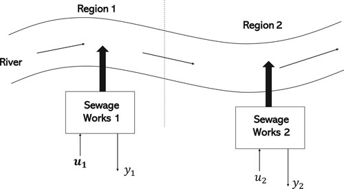
Assume that the river has two regions and each region has a sewage station. Then, the river pollution system can be described by a nonlinear interconnected systems as follows (see Yan et al., 2017 for no delay case) (38) $\begin{array}{rl}{\dot{x}}_1& =\underset{A_1}{\underbrace{\left[\begin{array}{cc}-1.32& 0\\ -0.32& -1.2\end{array}\right]}}{x}_1\\ & +\underset{B_1}{\underbrace{\left[\begin{array}{c}1\\ 0\end{array}\right]}}(u_1+\mathrm{\Delta }{g}_1(\cdot \left)\right)+h_1\left(x\right)\end{array}$(38) (39) $\begin{array}{rl}{y}_1& =\underset{C_1}{\underbrace{\left[\begin{array}{cc}1& 0\end{array}\right]}}{x}_1\end{array}$(39) (40) $\begin{array}{rl}{\dot{x}}_2& =\underset{A_2}{\underbrace{\left[\begin{array}{cc}-1.32& 0\\ -0.32& -1.2\end{array}\right]}}{x}_2+\underset{B_2}{\underbrace{\left[\begin{array}{c}1\\ 0\end{array}\right]}}(u_2+\mathrm{\Delta }{g}_2(\cdot \left)\right)+h_2\left(x\right)\end{array}$(40) (41) $\begin{array}{rl}{y}_2& =\underset{C_2}{\underbrace{\left[\begin{array}{cc}1& 0\end{array}\right]}}{x}_2\end{array}$(41) where $x_1=col(x_{11},x_{12})$, $x_2=col(x_{21},x_{22})$ and $x=col(x_1,x_2)$. The variables $x_{i1}$ and $x_{i2}$ for i = 1, 2 represent the concentration of biochemical oxygen demand (BOD) and the concentration of dissolved oxygen, respectively, the controllers $u_i$ are the BOD of the effluent discharge into the river, $\mathrm{\Delta }{g}_i$ represent any matched uncertainties and $h_i$ represent interconnections respectively for i = 1, 2. It is assumed that the concentrations of BOD for the two regions are measurable.

In this example, according to (5(5) $\begin{array}{rl}& {\dot{x}}_i=A_i{x}_i+f_i\left(x_i\right)+B_i(u_i+\mathrm{\Delta }{g}_i(x_i\left)\right)+h_i\left(x\right)\\ & y_i=C_i{x}_{i}i=1,2,\dots ,N\end{array}$(5) ), the nonlinear term $f_i\left(x_1\right)=0$, so Assumption 3.2 is not required. Moreover, it can be verified that $rank\left(C_i{B}_i\right)=1=m_i$ for i = 1, 2. So the Assumption 1 is satisfied. Some suitable coordinate transformation matrices $T_i$ are introduced as below ($z_i=T_i{x}_i$) $T_1=T_2=\left[\begin{array}{cc}0& 1\\ 1& 0\end{array}\right].$Then, the system (38(38) $\begin{array}{rl}{\dot{x}}_1& =\underset{A_1}{\underbrace{\left[\begin{array}{cc}-1.32& 0\\ -0.32& -1.2\end{array}\right]}}{x}_1\\ & +\underset{B_1}{\underbrace{\left[\begin{array}{c}1\\ 0\end{array}\right]}}(u_1+\mathrm{\Delta }{g}_1(\cdot \left)\right)+h_1\left(x\right)\end{array}$(38) )–(41(41) $\begin{array}{rl}{y}_2& =\underset{C_2}{\underbrace{\left[\begin{array}{cc}1& 0\end{array}\right]}}{x}_2\end{array}$(41) ) in z coordinates can be given by (42) $\begin{array}{rl}{\dot{z}}_1& =\underset{{\hat{A}}_1}{\underbrace{\left[\begin{array}{cc}-1.2& -0.32\\ 0& -1.32\end{array}\right]}}{z}_1\\ & +\underset{{\hat{B}}_1}{\underbrace{\left[\begin{array}{c}0\\ 1\end{array}\right]}}(u_1+\mathrm{\Delta }{G}_1(z_1\left)\right)+H_1\left(z\right)\end{array}$(42) (43) $\begin{array}{rl}{y}_1& =\underset{{\hat{C}}_1}{\underbrace{\left[\begin{array}{cc}0& 1\end{array}\right]}}{z}_1\end{array}$(43) (44) $\begin{array}{rl}{\dot{z}}_2& =\underset{{\hat{A}}_2}{\underbrace{\left[\begin{array}{cc}-1.2& -0.32\\ 0& -1.32\end{array}\right]}}{z}_2\\ & +\underset{{\hat{B}}_2}{\underbrace{\left[\begin{array}{c}0\\ 1\end{array}\right]}}(u_2+\mathrm{\Delta }{G}_1(z_1\left)\right)+H_2\left(z\right)\end{array}$(44) (45) $\begin{array}{rl}{y}_2& =\underset{{\hat{C}}_2}{\underbrace{\left[\begin{array}{cc}0& 1\end{array}\right]}}{z}_2\end{array}$(45) For simulation purpose, the matched uncertainties $\mathrm{\Delta }{G}_1(\cdot )$ and $\mathrm{\Delta }{G}_2(\cdot )$ are chosen to satisfy (46) $|\mathrm{\Delta }{G}_1(\cdot )|\le |-13.2z_{12}|,|\mathrm{\Delta }{G}_2(\cdot )|\le |{\cos }^2\left(z_{22}\right)|$(46) and the interconnected terms are set as (47) $\parallel H_1\parallel \le |z_{22}|,\parallel H_2\parallel \le |0.9z_{12}|.$(47) Combining (46(46) $|\mathrm{\Delta }{G}_1(\cdot )|\le |-13.2z_{12}|,|\mathrm{\Delta }{G}_2(\cdot )|\le |{\cos }^2\left(z_{22}\right)|$(46) )–(47(47) $\parallel H_1\parallel \le |z_{22}|,\parallel H_2\parallel \le |0.9z_{12}|.$(47) ), it is clear that Assumption 3.3 is satisfied. And the sliding surfaces $S_i$ are ${\dot{z}}_{i1}=-1.2z_{i1}-0.32z_{i2}.i=1,2$The initial states are chosen as $z_1\left(0\right)=col(0,1)$ and $z_2\left(0\right)=col(0,0)$, and the desired output signals $y_{id}$ are set as $y_{1d}=2e^{-t},y_{2d}=\sin \left(0.5t\right)+1.$It is clear that Assumption 3.4 is satisfied. Let $L_{12}=2,L_{22}=\mathrm{0.5.}$From (30(30) $\begin{array}{rl}{u}_i& =-B_{i2}^{-1}sgn\left(e_i\right)\{\parallel {\hat{A}}_{i21}{z}_{i1}\parallel +\parallel {\hat{A}}_{i22}{y}_i\parallel \\ & +\parallel F_{i2}(z_{i1},y_i)\parallel \\ & +\parallel {\hat{B}}_{i2}\parallel {\rho }_i(z_{i1},y_i)+k_i(z_{i1},y_i)+L_{i2}\}\end{array}$(30) ), the proposed sliding mode controllers are as follows (48) $\begin{array}{rl}{u}_1& =-sgn(y_1-y_{1d})(|1.32z_{12}|+|13.2z_{12}|+3)\end{array}$(48) (49) $\begin{array}{rl}{u}_2& =-sgn(y_2-y_{2d})(|1.32z_{22}|+|{\cos }^2(z_{22})|+2.3).\end{array}$(49) According to (9(9) ${\hat{A}}_{i11}^{\mathsf{T}}{P}_i+P_i{\hat{A}}_{i11}=-Q_i,i=1,2,\dots ,N.$(9) ), choose $Q_1=Q_2=1$. Combining (38(38) $\begin{array}{rl}{\dot{x}}_1& =\underset{A_1}{\underbrace{\left[\begin{array}{cc}-1.32& 0\\ -0.32& -1.2\end{array}\right]}}{x}_1\\ & +\underset{B_1}{\underbrace{\left[\begin{array}{c}1\\ 0\end{array}\right]}}(u_1+\mathrm{\Delta }{g}_1(\cdot \left)\right)+h_1\left(x\right)\end{array}$(38) )–(40(40) $\begin{array}{rl}{\dot{x}}_2& =\underset{A_2}{\underbrace{\left[\begin{array}{cc}-1.32& 0\\ -0.32& -1.2\end{array}\right]}}{x}_2+\underset{B_2}{\underbrace{\left[\begin{array}{c}1\\ 0\end{array}\right]}}(u_2+\mathrm{\Delta }{g}_2(\cdot \left)\right)+h_2\left(x\right)\end{array}$(40) ), $A_{i11}=-1.2$ for i = 1, 2. Then $P_1=P_2=\mathrm{0.416.}$By direct calculation, it follows from (24(24) $\begin{array}{r}{m}_{ij}=\{\begin{array}{ll}{\lambda }_{min}\left(Q_i\right)-\parallel R_i(\cdot )\parallel -2\parallel P_i\parallel {\gamma }_{i1}(\cdot ),& i=j\\ -2\parallel P_i\parallel {\gamma }_{i1}(\cdot ),& i\ne j\end{array}\end{array}$(24) ) that $\begin{array}{rl}& M^{\mathrm{\top }}+M\\ & =\left[\begin{array}{cc}-1.664{\gamma }_{11}+2& -0.832({\gamma }_{11}+{\gamma }_{21})\\ -0.832({\gamma }_{11}+{\gamma }_{21})& -1.664{\gamma }_{21}+2\end{array}\right].\end{array}$According to (23(23) $\begin{array}{rl}& \parallel H_{i1}(z_{11},y_{1d},\dots ,z_{N1},y_{Nd})\parallel \\ & \le {\gamma }_{i1}(\Vert T^{-1}col(z_{11},y_{1d},\dots ,z_{N1},y_{Nd}\Vert \left)\right)\\ & \times (\sum _{j=1}^N\parallel z_{j1}\parallel +\sum _{j=1}^N\parallel y_{jd}\parallel )\end{array}$(23) ), (42(42) $\begin{array}{rl}{\dot{z}}_1& =\underset{{\hat{A}}_1}{\underbrace{\left[\begin{array}{cc}-1.2& -0.32\\ 0& -1.32\end{array}\right]}}{z}_1\\ & +\underset{{\hat{B}}_1}{\underbrace{\left[\begin{array}{c}0\\ 1\end{array}\right]}}(u_1+\mathrm{\Delta }{G}_1(z_1\left)\right)+H_1\left(z\right)\end{array}$(42) ) and (44(44) $\begin{array}{rl}{\dot{z}}_2& =\underset{{\hat{A}}_2}{\underbrace{\left[\begin{array}{cc}-1.2& -0.32\\ 0& -1.32\end{array}\right]}}{z}_2\\ & +\underset{{\hat{B}}_2}{\underbrace{\left[\begin{array}{c}0\\ 1\end{array}\right]}}(u_2+\mathrm{\Delta }{G}_1(z_1\left)\right)+H_2\left(z\right)\end{array}$(44) ), ${\gamma }_{11}=6\cdot {\sin }^2\left(z_{11}\right),{\gamma }_{21}=2\cdot \cos \left(z_{21}\right)+3.$By direct verification, it is straightforward to check that $M^{\mathrm{\top }}+M>0$ in the domain Ω of the origin satisfying $\mathrm{\Omega }=\left\{\right(z_{11},z_{21},\dots ,z_{N1})||z_{11}|\le 5.2\mathrm{\&}\Vert z_{21}|\le 3.9\}$.

According to (27(27) $\begin{array}{rl}& \dot{V}(z_{11},z_{21},\dots ,z_{N1})\\ & \le \sum _{i=1}^N\{-{\lambda }_{min}(Q_i)\parallel z_{i1}{\parallel }^2+\parallel {\mathrm{\Gamma }}_{i11}(z_{i1},y_{id}{)}^{\mathsf{T}}{P}_i\\ & +P_i{\mathrm{\Gamma }}_{i11}(z_{i1},y_{id})\parallel \parallel z_{i1}{\parallel }^2\\ & +2\parallel z_{i1}\parallel \parallel P_i\parallel \parallel {\hat{A}}_{i12}{y}_{id}\parallel \\ & +2\parallel z_{i1}\parallel \parallel P_i\parallel \parallel {\mathrm{\Gamma }}_{i12}(z_{i1},y_{id})y_{id}\parallel \\ & +2\parallel z_{i1}\parallel \parallel P_i\parallel \parallel H_{i1}(z_{11},y_{1d},\dots ,z_{N1},y_{Nd})\parallel \}\\ & =-\sum _{i=1}^N\{{\lambda }_{min}\left(Q_i\right)-\parallel R_i(\cdot )\parallel \\ & -2\parallel P_i\parallel {\gamma }_{i1}(\cdot )\}\parallel z_{i1}{\parallel }^2\\ & +2\sum _{i=1}^N\sum _{\begin{array}{c}j=1\\ j\ne i\end{array}}^N\parallel P_i\parallel \parallel z_{i1}\parallel {\gamma }_{i1}(\cdot )(\parallel z_{j1}\parallel +L_{i1})\\ & +2\sum _{i=1}^N(\parallel {\hat{A}}_{i12}{y}_{id}\parallel +\parallel {\mathrm{\Gamma }}_{i12}(z_{i1},y_{id})y_{id}\parallel )\\ & \cdot \parallel P_i\parallel \parallel z_{i1}\parallel \\ & \le -\frac{1}{2}{\lambda }_{min}(M^{\mathsf{T}}+M)\sum _{i=1}^N\parallel z_{i1}{\parallel }^2\\ & +2\sum _{i=1}^N(\parallel {\hat{A}}_{i12}{y}_{id}\parallel +\parallel {\mathrm{\Gamma }}_{i12}(z_{i1},y_{id})y_{id}\parallel \\ & +{\gamma }_{i1}(\cdot )L_{i1})\cdot \parallel P_i\parallel \parallel z_{i1}\parallel \\ & =-\frac{1}{2}\sum _{i=1}^N\left\{{\lambda }_{min}\right(M^{\mathsf{T}}+M)\parallel z_{i1}\parallel \\ & -4(\parallel {\hat{A}}_{i12}{y}_{id}\parallel +\parallel {\mathrm{\Gamma }}_{i12}(z_{i1},y_{id})y_{id}\parallel \\ & +{\gamma }_{i1}(\cdot )L_{i1})\parallel P_i\parallel \}\parallel z_{i1}\parallel \end{array}$(27) ) for this example (50) $\dot{V}(z_{11},z_{21})\le 0$(50) if $|z_{11}|\ge 0.3$ and $|z_{21}|\ge 0.25$. Therefore, system (38(38) $\begin{array}{rl}{\dot{x}}_1& =\underset{A_1}{\underbrace{\left[\begin{array}{cc}-1.32& 0\\ -0.32& -1.2\end{array}\right]}}{x}_1\\ & +\underset{B_1}{\underbrace{\left[\begin{array}{c}1\\ 0\end{array}\right]}}(u_1+\mathrm{\Delta }{g}_1(\cdot \left)\right)+h_1\left(x\right)\end{array}$(38) )–(41(41) $\begin{array}{rl}{y}_2& =\underset{C_2}{\underbrace{\left[\begin{array}{cc}1& 0\end{array}\right]}}{x}_2\end{array}$(41) ) is uniformly ultimately bounded.

The tracking results are shown in Figure 2, which offers a high tracking performance. The concentration of biochemical oxygen demand (BOD) of each subsystem $y_i$ can track the ideal reference $y_{id}$ using the controller from (48(48) $\begin{array}{rl}{u}_1& =-sgn(y_1-y_{1d})(|1.32z_{12}|+|13.2z_{12}|+3)\end{array}$(48) )–(49(49) $\begin{array}{rl}{u}_2& =-sgn(y_2-y_{2d})(|1.32z_{22}|+|{\cos }^2(z_{22})|+2.3).\end{array}$(49) ), even in the presence of uncertainties. The time responses of the states of the system (38(38) $\begin{array}{rl}{\dot{x}}_1& =\underset{A_1}{\underbrace{\left[\begin{array}{cc}-1.32& 0\\ -0.32& -1.2\end{array}\right]}}{x}_1\\ & +\underset{B_1}{\underbrace{\left[\begin{array}{c}1\\ 0\end{array}\right]}}(u_1+\mathrm{\Delta }{g}_1(\cdot \left)\right)+h_1\left(x\right)\end{array}$(38) )–(41(41) $\begin{array}{rl}{y}_2& =\underset{C_2}{\underbrace{\left[\begin{array}{cc}1& 0\end{array}\right]}}{x}_2\end{array}$(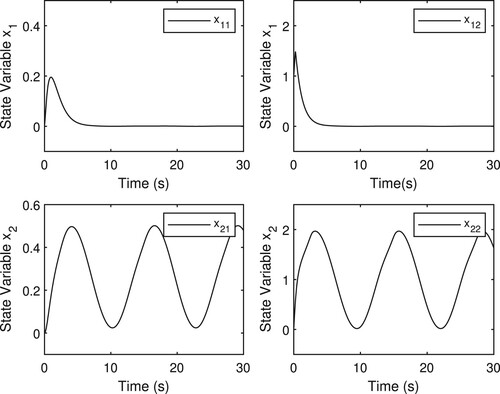41) ) are shown in Figure 3. which indicates that the system states are bounded. Simulation results demonstrate that the method developed in this paper is effective.

Figure 2. Time responses of system outputs and desired outputs.

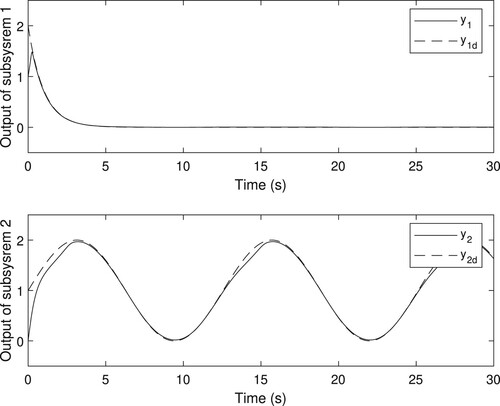
Figure 3. Time responses of system state variables.

7. Conclusions

This paper has presented a sliding mode control strategy to deal with the output tracking problem of a class of large-scale systems with unmatched unknown nonlinear interconnections. The desired reference signals are allowed to be time-varying. A decentralised sliding mode control scheme has been proposed to satisfy the reachability condition. This drives the interconnected system onto the pre-designed sliding surface. A set of conditions is developed to guarantee that the output tracking errors are uniformly ultimately bounded while all the state variables of the interconnected system are bounded. The application of the developed results to a river pollution control system has demonstrated that the proposed approach is effective and practicable.

Disclosure statement

No potential conflict of interest was reported by the author(s).

Data availability statement

The authors confirm that the data supporting the findings of this study are available within the article.

Additional information

Funding

This work was supported by the National Natural Science Foundation of China [grant numbers 61922042 and 62020106003], China Scholarship Council for 3 years' study at the University of Kent, and Qing Lan Project.

Notes on contributors

Yueheng Ding

Yueheng Ding received the B.S. degree in electrical engineering and automation from the Jiangsu Normal University, Jiangsu, P.R. China, in 2018. He is currently a PhD candidate in electronic engineering at University of Kent, Canterbury, UK. His research interests include tracking control, sliding mode control, decentralized control and large-scale interconnected systems.

Xinggang Yan

Dr Xinggang Yan received the B.Sc. Degree from Shaanxi Normal University, in 1985, the M.Sc. Degree from Qufu Normal University in 1991, and the Ph.D. Degree of Engineering from Northeastern University, China in 1997. Currently, he is Senior Lecturer in Control Engineering at the University of Kent, United Kingdom. He received the Best Application Paper Award of ASian Control Conference (ASCC) in Fukuoka, Japan in 2019. He has published three books, six invited book chapters and about 200 referred papers in the area of control engineering. He serves as the Associate Editor for several engineering journals including IET Control Theory & Applications, Energies, and Complexity. His research interests include decentralised control, sliding mode control, fault detection and isolation, time delay systems and interconnected systems.

Zehui Mao

Professor Zehui Mao (M'10) received her Ph.D. degree in Control Theory and Control Engineering from Nanjing University of Aeronautics and Astronautics, Nanjing, China, in 2009. She is currently a professor at the College of Automation Engineering in Nanjing University of Aeronautics and Astronautics, China. She was a visiting scholar in University of Virginia. She worked in the areas of fault diagnosis, with particular interests in nonlinear control systems, sampled-data systems and networked control systems. Her current research interests include fault diagnosis and fault-tolerant control of systems with disturbance and incipient faults, and high speed train and spacecraft flight control applications.

Bin Jiang

Bin Jiang (M'03-SM'05-F'20) received the Ph.D. degree in automatic control from Northeastern University, Shenyang, China, in 1995. He is currently Chair Professor of Cheung Kong Scholar Program with the Ministry of Education and the Vice President of Nanjing University of Aeronautics and Astronautics, Nanjing, China. He has authored eight books and over 200 referred international journal papers and conference papers. His current research interests include intelligent fault diagnosis and fault tolerant control and their applications to helicopters, satellites, and high-speed trains.

Dr. Jiang currently serves as an Associate Editor or an Editorial Board Member for a number of journals, such as the IEEE Trans. On Cybernetics, Neurocomputing al, He is a Chair of Control Systems Chapter in IEEE Nanjing Section, a member of IFAC Technical Committee on Fault Detection, Supervision, and Safety of Technical Processes.

Sarah K. Spurgeon

Sarah K. Spurgeon OBE, FREng, FIEEE, FIET obtained a BSc in Mathematics and a DPhil in Electronics from the University of York, UK in 1985 and 1988 respectively. She has held previous academic positions at the University of Loughborough, the University of Leicester and the University of Kent in the UK and is now Professor of Control Engineering and Head of the Department of Electronic and Electrical Engineering at University College London. Her research interests are in the area of systems modelling and analysis, robust control and estimation in which areas she has published over 270 refereed research papers. She was awarded the Honeywell International Medal for ‘distinguished contribution as a control and measurement technologist to developing the theory of control’ in 2010 and an IEEE Millenium Medal in 2000. She is currently Vice President Publications of the International Federation of Automatic Control (IFAC), an elected member of the Board of Governors of the IEEE Control Systems Society and a member of the General Assembly of the European Control Association. Within the UK she is currently a Vice President of the IET and is a past President of the Engineering Professors Council, the representative body for engineering in higher education.

References

- Cai, H., & Hu, G. (2017). Distributed tracking control of an interconnected leader–follower multiagent system. IEEE Transactions on Automatic Control, 62(7), 3494–3501. https://doi.org/10.1109/TAC.2017.2660298
- Edwards, C., & Spurgeon, S. K. (1998). Sliding mode control theory and application. Taylor & Francis.
- Farzad, Z., & Mohammad Hossein, S. (2018). On event-triggered tracking for non-linear SISO systems via sliding mode control. IMA Journal of Mathematical Control and Information, 37(1), 105–119. https://doi.org/10.1093/imamci/dny041
- Han, Y. Q., & Yan, H. S. (2020). Observer-based multi-dimensional Taylor network decentralised adaptive tracking control of large-scale stochastic nonlinear systems. International Journal of Control, 93(7), 1605–1618. https://doi.org/10.1080/00207179.2018.1521994
- Huerta, H., Loukianov, A. G., & Cañedo, J. M. (2019). Passivity sliding mode control of large-scale power systems. IEEE Transactions on Control Systems Technology, 27(3), 1219–1227. https://doi.org/10.1109/TCST.87
- Kim, H. S., Park, J. B., & Joo, Y. H. (2017). Decentralized sampled-data tracking control of large-scale fuzzy systems: an exact discretization approach. IEEE Access, 5, 12668–12681. https://doi.org/10.1109/ACCESS.2017.2723982
- Li, X. H., & Liu, X. P. (2018). Backstepping-based decentralized adaptive neural H∞ tracking control for a class of large-scale nonlinear interconnected systems. Journal of the Franklin Institute, 355(11), 4533–4552. https://doi.org/10.1016/j.jfranklin.2018.04.038
- Liu, C., Zhang, H., Xiao, G., & Sun, S. (2019). Integral reinforcement learning based decentralized optimal tracking control of unknown nonlinear large-scale interconnected systems with constrained-input. Neurocomputing, 323, 1–11. https://doi.org/10.1016/j.neucom.2018.09.011
- Lunze, J. (2020). Feedback control of large-scale systems. Bookmundo Direct.
- Onyeka, A. E., Yan, X. G., Mao, Z., Jiang, B., & Zhang, Q. (2020). Robust decentralised load frequency control for interconnected time delay power systems using sliding mode techniques. IET Control Theory and Applications, 14(2), 470–480. https://doi.org/10.1049/cth2.v14.3
- Pagilla, P. R., Dwivedula, R. V., & Siraskar, N. B. (2007). A decentralized model reference adaptive controller for large-scale systems. IEEE/ASME Transactions on Mechatronics, 12(2), 154–163. https://doi.org/10.1109/TMECH.2007.892823
- Ren, X., Yang, G., & Li, X. (2020). Global adaptive fuzzy distributed tracking control for interconnected nonlinear systems with communication constraints. IEEE Transactions on Fuzzy Systems, 28(2), 333–345. https://doi.org/10.1109/TFUZZ.91
- Rinaldi, G., Menon, P. P., Edwards, C., & Ferrara, A. (2019). Variable gains decentralized super-twisting sliding mode controllers for large-scale modular systems. In 2019 18th European control conference (ECC) (pp. 3577–3582).
- Ruiz-Duarte, J., & Loukianov, A. (2020). Approximate causal output tracking for linear perturbed systems via sliding mode control. International Journal of Control, 93(4), 993–1004. https://doi.org/10.1080/00207179.2018.1500034
- Song, J., Huang, L. Y., Karimi, H. R., Niu, Y., & Zhou, J. (2020). ADP-based security decentralized sliding mode control for partially unknown large-scale systems under injection attacks. IEEE Transactions on Circuits and Systems I: Regular Papers, 67(12), 5290–5301. https://doi.org/10.1109/TCSI.8919
- Song, J., Wang, Y. K., Niu, Y., Lam, H. K., He, S., & Liu, H. (2022). Periodic event-triggered terminal sliding mode speed control for networked PMSM system: A GA-optimized extended state observer approach. IEEE/ASME Transactions on Mechatronics. Advance Online Publication. https://doi.org/10.1109/TMECH.2022.3148541
- Su, Z., Qian, C., Hao, Y., & Zhao, M. (2018). Global stabilization via sampled-data output feedback for large-scale systems interconnected by inherent nonlinearities. Automatica, 92, 254–258. https://doi.org/10.1016/j.automatica.2018.03.057
- Tan, L. N. (2020). Distributed H∞ optimal tracking control for strict-feedback nonlinear large-scale systems with disturbances and saturating actuators. IEEE Transactions on Systems, Man, and Cybernetics: Systems, 50(11), 4719–4731. https://doi.org/10.1109/TSMC.6221021
- Wan, M., & Yin, Y. (2020). Adaptive decentralized output feedback tracking control for large-scale interconnected systems with time-varying output constraints. Mathematical Problems in Engineering, 2020. https://doi.org/10.1155/2020/6760521
- Wei, Y., Zheng, Z., Li, Q., Jiang, Z., & Yang, P. (2020). Robust tracking control of an underwater vehicle and manipulator system based on double closed-loop integral sliding mode. International Journal of Advanced Robotic Systems, 17(4), 172988142094177. https://doi.org/10.1177/1729881420941778
- Wu, L. B., Wang, H., He, X. Q., & Zhang, D. Q. (2018). Decentralized adaptive fuzzy tracking control for a class of uncertain large-scale systems with actuator nonlinearities. Applied Mathematics and Computation, 332, 390–405. https://doi.org/10.1016/j.amc.2018.03.080
- Wu, S. F., Grimble, M. J., & Breslin, S. G. (1998). Introduction to quantitative feedback theory for lateral robust flight control systems design. Control Engineering Practice, 6(7), 805–828. https://doi.org/10.1016/S0967-0661(98)00053-7
- Yan, X., Spurgeon, S., & Edwards, C. (2014). Memoryless static output feedback sliding mode control for nonlinear systems with delayed disturbances. IEEE Transactions on Automatic Control, 59(7), 1906–1912. https://doi.org/10.1109/TAC.9
- Yan, X., Spurgeon, S., & Edwards, C. (2017). Variable structure control of complex systems: analysis and design. Springer.
- Yan, X. G., Edwards, C., & Spurgeon, S. K. (2004). Decentralised robust sliding mode control for a class of nonlinear interconnected systems by static output feedback. Automatica, 40(4), 613–620. https://doi.org/10.1016/j.automatica.2003.10.025
- Yan, X. G., Lam, J., & Dai, G. Z. (1999). Decentralized robust control for nonlinear large-scale systems with similarity. Computers & Electrical Engineering, 25(3), 169–179. https://doi.org/10.1016/S0045-7906(99)00002-6
- Yan, X. G., Wang, J. J., Lu, X. Y., & Zhang, S. Y. (1998). Decentralized output feedback robust stabilization for a class of nonlinear interconnected systems with similarity. IEEE Transactions on Automatic Control, 43(2), 294–299. https://doi.org/10.1109/9.661085
- Yan, Y., Yu, S. H., & Sun, C. Y. (2020). Quantization-based event-triggered sliding mode tracking control of mechanical systems. Information Sciences, 523, 296–306. https://doi.org/10.1016/j.ins.2020.03.023
- Yao, D., Li, H., Lu, R., & Shi, Y. (2020). Distributed sliding-mode tracking control of second-order nonlinear multiagent systems: an event-triggered approach. IEEE Transactions on Cybernetics, 50(9), 3892–3902. https://doi.org/10.1109/TCYB.6221036
- Zhao, B., Liu, D., Xiong, Y., & Li, Y. C. (2017). Observer-critic structure-based adaptive dynamic programming for decentralised tracking control of unknown large-scale nonlinear systems. International Journal of Systems Science, 48(9), 1978–1989. https://doi.org/10.1080/00207721.2017.1296982
- Zhao, Y., Sun, X., Wang, G., & Fan, Y. (2021). Adaptive backstepping sliding mode tracking control for underactuated unmanned surface vehicle with disturbances and input saturation. IEEE Access, 9, 1304–1312. https://doi.org/10.1109/Access.6287639
- Zhu, G., Nie, L., Lv, Z., Sun, L., Zhang, X., & Wang, C. (2020). Adaptive fuzzy dynamic surface sliding mode control of large-scale power systems with prescribe output tracking performance. ISA Transactions, 99, 305–321. https://doi.org/10.1016/j.isatra.2019.08.063