Model-free robust decoupling control of nonlinear nonaffine dynamic systems

Abstract

This study presents a model-free robust input-output decoupling control with Nonlinear-Dynamic-Coupling Inversion/Inverter (NDCI) in a U-control framework. Regarding the decoupling, an input/output (I/O) coupling matrix function is proposed to derive two decouplers (U-decoupler/functional inversion and D-decoupler/static matrix inversion). A general existing theorem is proved for model-free sliding mode control (MFSMC) to lay the foundation for the NDCI, which takes the Lyapunov differential inequality for its derivative rather than the semi-define Lyapunov derivative. Accordingly, a multi-input and multi-output (MIMO) model-free decoupling U-control (MFDUC) platform is established to integrate the functionalities into a double closed-loop system framework. To validate the functionalities and configurations, this study presents transparent and comparative simulated bench tests, which also could be treated as user guidance for further study and ad hoc applications.

KEYWORDS:

• MIMO decoupling control
• model-free SMC
• I/O model-based/free decoupling
• nonlinear-dynamic-coupling inversion/inverter (NDCI)
• U-control framework
• simulation validations

1. Introduction

Control of MIMO dynamic systems has been naturally widely rooted in academic research and industrial applications (Liu et al., 2019; Novara & Milanese, 2019; Wu et al., 2022; Ye & Song, 2022), which has been continuously reported in textbooks (Bhattacharyya & Keel, 2022; Isidori, 2014; Wang et al., 2008) and journal publications (Celentano et al., 2020; Rodrigues & Mesbah, 2021; Ye & Song, 2022). A critical bottleneck issue for this type of control system design, compared with SISO systems, is the coupling of input/output (I/O) — the interactions between the two ends. Accordingly, decoupling is a straightforward intuition for designing MIMO control systems because it is simple and effective for designing controllers to achieve the system I/O pairing performance/operation with SISO techniques. Bearing the size of the study, it cannot cover the enormous achievements in MIMO control system design. Accordingly, with the focus of the study, it only takes a critical review of some of the representative decoupling methods to justify the study motivation and to outline the major contributions of the study.

Model-based decoupling control: Most of the decoupling control has been linear model-based, which makes a plant into a diagonal matrix to facilitate using the SISO design techniques for the control system into independently paired I/O in operation. Representatively, various transfer function-based dynamic decoupling control schemes have been presented (Cai et al., 2008), which convert the plant into diagonally expanded matrices through pre-compensators. Similar decoupling approaches, such as band-decoupled and statically decoupled systems and triangularly coupled systems (Dumont, 2021), have been studied as well. For the state space model-based decoupling control, the design is formulated in terms of a state feedback controller and feedforward gain controller to achieve diagonalised I/O pairing effects while simultaneously obtaining the other specified system performance (Zhao et al., 2021). For nonlinear model-based decoupling control, most of the studies do not directly take the nonlinear plant model for decoupling (maybe generally impossible for nonlinear decoupling), alternatively use other techniques such as coordinate transform or deliberately treat the nonlinear coupling as uncertainty/external disturbance (Zhu & Wang, 2020), linearisation of nonlinear models (Mao et al., 2011; Pandey et al., 2021). While a nonlinear model is used for decoupling design, the formulations are much more complicated (Nijmeijer & Respondek, 1988). Studies on nonlinear model-based decoupling control have been mainly linked to applications, but no obvious progression in methodology development recently. In summary, model-based decoupling approaches have obvious merit in dealing with interaction functional analysis and algorithm formulation; however, on the other side, it has less robustness (sensitive to plant model uncertainty) and is difficult in solving equation systems, possibly even transcendental, nonlinear equations with nonlinear I/O coupled plants, further the control systems need re-design once the nominal models changed. This gives the first motivation in considering model-free style decoupling control to increase the robustness and remove the equation-based functional decoupling.

Model-free decoupling control: Price and Rasmussen (2017) presented a high-gain-based cascade control to implement model-free decoupling control of heating, ventilation and air conditioning (HAVC) systems, which need mild conditions to approximate nonlinear dynamic plus cautiousness in selecting the inner loop gain. The other most closely claimed model-free decoupling control has been adaptive and/or neural network based data-driven approaches (Dai et al., 2001; Zhou et al., 2023), which adaptively use universal approximation and online (i.e. real-time) learning to determine data-driven models as reference for controller design. Picking up a few exemplary publications to show the research progressions in this domain, Wang et al. (2009) proposed a model-free indirect adaptive decoupling control for nonlinear discrete-time MIMO systems, which obviously involved adaptive modelling and linearisation for decoupling control. Hou et al. (2021) proposed a data-driven discrete terminal sliding mode decoupling control method with prescribed performance, again obviously data-driven linearisation model was used to derive the decoupling control. The other interesting topic is considering the randomness of the data-driven approach, in which the data-driven decoupling design has been investigated in probability using mutual information optimisation (Zhang & Zhou, 2022), which deals with couplings among the outputs of the stochastic systems (Zhang & Wang, 2017). An open space for further study is to remove the request of the nominal model base for the PI controller design and the feasibility to remove the request for probability density functions in the decoupling controller design.

However, strictly speaking, the above configurations cannot be deemed as strict model-free style, because of using online estimated models in decoupling. Therefore, an obvious question asked here is why there is almost no proper solution for mode-free decoupling control so far. From the author’s point of view, this is not because the topic is meaningless, it is essentially because there is no proper insight/configuration/formulation. Consequently, this gives rise to the second motivation of the study for decoupling control without using both offline models and adaptive online models.

U-control system framework: U-control has been predominantly developed for SISO control system design, analysis and simulation. The U-control framework has structures with two loops, the inner loop for trimming the plant to achieve nonlinear dynamic inversion into a unit constant or an identity matrix and the outer loop for achieving system performance. Accordingly, the control design tasks are relieved via plant stabilisation/inversion in the inner loop and system performance specification in the outer loop separately, which makes the control system design universally feasible for all the model-based and model-free dynamic plants. It should be noted that in parallel the high-order fully actuated system control approach (Duan, 2021) is the equivalent design of a model-based U-control, while a control/input affine nonlinear model is used.

The kernel foundation of the U-control methodology is the double dynamic inversion to separate the request of stabilisation and response performance, which provides simplicity/generality (solutions) from complexity (problems). Some representative publications include model-based discrete time U-control (Zhu & Guo, 2002) achieving general pole placement control by the integration of solving Diophantine equation and U-inversion; a general procedure for dynamic inversion (Li et al., 2020); U-model, U-control methodology and platform (Zhang et al., 2020); underactuated coupled nonlinear adaptive control synthesis using the U-model for multivariable unmanned marine robotics (Hussain et al., 2020); complete model-free sliding mode control (CMFSMC) (Zhu, 2021; Zhu et al., 2022); a new configuration of composite nonlinear feedback control (Zhu et al., 2023); robust trajectory tracking of quadrotor UAV using U-control (Li et al., 2022). It should be noted that no decoupling control approach included in the framework so far. Consequently, the inclusion of this type of multi-variable U-control is the third motivation of the study.

Justification of the study

In brief, the bottleneck issue of the study is how the SISO MFSMC approach can accommodate the third inversion – input-output decoupling based on the nonlinear and dynamic inversions while treating the plant as a complete uncertainty. From the conceptual understanding and technical configuration, to the derivation of the formulation are critically challenging, maybe this is why no such work appeared before the study, rather because this topic is trivial and not worthwhile make it.

Motived from the above critical review, verbally, the study presents a new approach to cancel the I/O coupling to simplify the MIMO control system design procedure and to improve the resultant performances, in terms of robustness (model-free), generality (model-free), simplicity in design and implementation (U-control, model-free SMC, double dynamic inversion, model-free decoupling) and bench tests for understanding and applications. The major contributions from the study are outlined below.

1. To achieve a decoupling effect, an I/O-coupling control matrix function (I/O-CCMF) is proposed to form a basis for decoupling design, which enables two decouplers derived, one is the U-decoupler by solving the I/O-CCMF and the other is the D-decoupler by taking a gain matrix inversion. Integrating the two decouplers with the Nonlinear-Dynamic-Inversion (NDI) within a closed loop significantly reduces the design and computational complexity while increasing the robustness to uncertainties.

2. An SMC existing theorem is proved to generalise SMC in both forms, model-based and model-free formulations, by which the Lyapunov stability inequality is applied to obtain the switching and equivalent controls without inducing chattering effects.

3. To accommodate the MIMO decoupling control, the dual loop SISO U-control platform, composed of plant trimming in the inner loop with stabilisation/robustness and assigning system performance (e.g. damping ratio and undamped natural frequency) in the outer loop, are properly expanded to cover the multi-variable control systems.

4. Simulation studies, with significantly input/output coupled nonlinear nonaffine dynamic plants, are conducted not only to validate the functional configurations and analytical results  but also to provide transparent guidance for future expansions/applications.

5. This presents an exemplary case study in terms of (1) a new vision of model-free control without using adaptive and/or data-driven online models, (2) a seamless supplement to model-based approaches, such as significantly reducing complexity in decoupling nonlinear control system design and real implementation, (3) an insight/definition for total robustness control, taking total uncertain systems (model-free), contrast to nominal model-based uncertain systems (still model-based), into analysis and design.

The rest of the study includes the following. Section 2 gives preliminary materials for the following section development, Section 3 presents the major analytical derivations and conceptual explanations for the model-free nonlinear-dynamic-coupling inversion/inverter (NDCI), Section 4 establishes the MIMO model-free decoupling U-control (MFDUC) platform, Section 5 takes up case studies through simulation demonstrations and comparisons with two bench test examples and Section 6 concludes the study.

2. Preliminary

2.1. Nonlinear plant description

Consider a class of general single-input single-output (SISO) nth-order nonlinear dynamic plant, described by (1) $\sum {}_{\text{SISO}}\text{: }{y}^{(n)}=f(y^{(0\sim n-1)},u,d)$(1) where the triplets {$y\in \mathsf{R}$, $u\in \mathsf{R}$ and $d\in \mathsf{R}$} are the plant output, input and external disturbance, respectively, and $y^{(0\sim n-1)}=[y\cdots y^{(n-1)}{]}^T\in {\mathsf{R}}^n$ is the $n-1$ order output derivative vector. It should be noted that model (1) can be expressed in state space equations as well by letting $x=y^{(0\sim n-1)}={\left[\begin{array}{cccc}{x}_1=y& x_2=\dot{y}& \cdots & x_{n-1}=y^{(n-1)}\end{array}\right]}^T\in {\mathsf{R}}^n$ and $x_n=f(x,u,d)$.

Assumption 2.1: $f:u\to y$, an unknown mapping from the input space to the output space, is a continuously differentiable of class ${\mathsf{C}}^n$ and satisfied with the Lipschitz continuity $|f(x_1)-f(x_2)|\le K|x_1-x_2|,K\in {\mathsf{R}}^{+}$.

Assumption 2.2: The plant is Bounded-Input-Bounded-Output (BIBO), $|u(t)|\le B_u\cap |y(t)|\le B_y,\mathrm{\forall }t\in {\mathsf{R}}^{+},B_u,B_y\in {\mathsf{R}}^{+}$.

Assumption 2.3: The plant is a class of asymptotically stable zero dynamics, which have minimum phase properties. Therefore, plant invertibility exists and is stable.

Assumption 2.4: The plant is completely observable/controllable, and the observability/controllability matrices are non-singular.

Assumption 2.5: The disturbance is unknown but bounded $|d|\le D=sup(|d|)\in {\mathsf{R}}^{+}$.

Remark 2.1:

This study treats the plant as a total uncertainty, except the dynamic order is assumingly known in the design and will expand this SISO description (1) into an MIMO template for developing model-free decoupling control in the following sections.

2.2. Generalised MFSMC

Regarding model (1), a generalised SISO SMC in the form of equivalent control can be expressed (Zhu, 2021). (2) $\begin{array}{rl}\sigma (\tilde{\mathrm{y}})& =\mu (\tilde{\mathrm{y}}),{\mathsf{R}}^n\to \mathsf{R}\\ \dot{\sigma }& =u=\{\begin{array}{ll}{u}_{sw}=-k_g\mathrm{sgn}(\sigma )& \mathrm{\forall }|\sigma |>\delta \\ u_{eq}={\rho (\sigma )|}_{\dot{\sigma }\sigma =0\cup \dot{\sigma }\sigma <0}& \mathrm{\forall }|\sigma |\le \delta \end{array}\text{, }\\ & {\mathsf{R}}^m\to \mathsf{R}\end{array}$(2) where $\sigma$ and $\dot{\sigma }$ are the sliding function (SF) and the derivative, respectively, $\tilde{\mathrm{y}}=\text{y}-{\text{y}}_d={\left[\begin{array}{cccc}\tilde{y}& \dot{\tilde{y}}& \cdots & {\tilde{y}}^{(n-1)}\end{array}\right]}^T\in {\mathsf{R}}^n$ is the output tracking error vector, $\text{y}=y^{(0\sim n-1)}={\left[\begin{array}{cccc}y& \dot{y}& \cdots & y^{(n-1)}\end{array}\right]}^T\in {\mathsf{R}}^n$ and ${\text{y}}_d={\left[\begin{array}{cccc}{y}_d& {\dot{y}}_d& \cdots & y_d^{(n-1)}\end{array}\right]}^T\in {\mathsf{R}}^n$ are the output derivative vector and the desired output derivative vector, respectively. $\mu (\tilde{\mathrm{y}})=0$ is a stable polynomial, such as satisfying Hurwitz stability and $\delta \in \mathsf{R}$ is the sliding band thickness. For model-based SMC, it gives $\dot{\sigma }=u=\rho (\sigma ){|}_{\dot{\sigma }\sigma =0}:{\mathsf{R}}^n\to \mathsf{R}$ and for the model-free SMC (MFSMC), it has $\dot{\sigma }=u=\rho (\sigma ){|}_{\dot{\sigma }\sigma <0}:{\mathsf{R}}^n\to \mathsf{R}$. This study will prove the MFSMC existing theorem and integrate it with MIMO model-free nonlinear dynamic inversion and decoupling control.

2.3. SISO model-free U-control systems

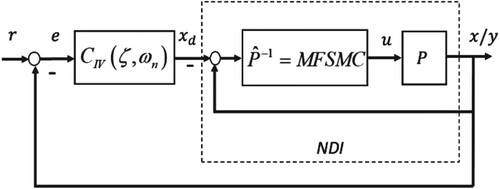
Figure 1 shows the SISO model-free U-control system, which is functionally expressed as (Zhu, 2021). (3) $\begin{array}{rl}& {\mathrm{\Sigma }}_{\text{Usiso}}:(F,C(C_{IV},{\hat{P}}^{-1}),P)\\ & \iff (F,C_{IV},C_{NDI}({\hat{P}}^{-1},P)\in I_n)\\ & \iff (F,C_{IV},I_n)\end{array}$(3) where F denotes the configuration of the U-control system. For a general model unknown plant $P\in {\mathsf{R}}^n$, the objective of the U-control system is to use a double loop of control configuration and design independently the controllers with double dynamic inversion formulations (the plant dynamic inversion in the inner loop and closed-loop control performance dynamic inversion in the outer loop). The two loop controllers are explained below.

1. Trimming plant: The control objective with the inner loop is to use model-free sliding mode control (MFSMC) ${\hat{P}}^{-1}=\text{MFSMC}$ to achieve nonlinear dynamic inversion/cancellation (NDI) to generate the nth-order identity matrix $C_{\text{NDI}}({\hat{P}}^{-1},P)\in I_n$ or a unit constant in terms of robust stability. It should be explained that (1) the design does not intend to achieve more specifications of the whole system response trajectory against nominal design performance, (2) while a plant converted to a unit constant/matrix in the inner loop, the controller design in the outer loop will be independently conducted without dealing with the plant/model, accordingly, named as invariant (IV) controller, (3) for SMC, if full states are unavailable, various state observers (Kang et al., 2013) are optional, for example, extended state observer (ESO) (Guo & Zhao, 2011), to estimate the state estimate from the control input and the measured system output.

2. Assigning system performance: The control objectives with the outer loop are (1) to use a closed loop to achieve nominal design performance, for example, linear dynamic system performance is specified with the Laplace transfer function $\frac{Y}{R}=G=\frac{C_{IV}}{1+C_{IV}}$, it can be implemented by a closed loop configuration while taking up the invariant controller $C_{IV}=(1-G{)}^{-1}G$, which is more robust, for sensitivity (Arkun et al., 1984), against the open-loop implementation, particularly to the commonly encountered constant disturbance, (2) to assign the closed-loop bandwidth narrower than that in the inner loop, (3) to use the invariant controller to provide the desired state vector or the desired output derivative vector as reference for the inner loop SMC.

This study will expand the SISO control framework to include the MIMO decoupling control.

Figure 1. Model-free SISO U-control platform.

Remark 2.2:

The similar idea using a dual loop to allocate control tasks has been adopted in adaptive tuning PID control (Huang et al., 2002). To gain the system’s robust stability in the inner loop tunes the controller online without seeking the nominal design performance. The outer loop takes periodic online detection when modelling errors occur and retune the controller. With such distributed control tasks, the system is treated as a newly configured system to provide effective control performance directly. This is also the U-control configuration with double loops. However, the obvious distinction is that U-control takes robust NDI in the inner loop, accordingly, the outer loop design with the nominal performance is completely independent of the inner loop, also the model-free U-control does not require adaptively estimating online models and extracting recursive information for designing controllers. The other approach, the high-order fully actuated (HOFA) control system design (Duan, 2021) as equivalently shown in the U-control framework Figure 2, is a type of model-based dynamic inversion control. For easy reference, the following notations are used to connect HOFA control with those functional blocks in U-control Figure 2.

1. The HOFA plant model $P:x^{(n)}=f(x^{(0\sim n-1)})+B(x^{(0\sim n-1)})u$

2. The model-based HOFA dynamic investigation $P^{-1}:u=-B^{-1}(f(x^{(0\sim n-1)})+A_{0\sim n-1}{x}^{(0\sim n-1)}-v)$

3. The invariant HOFA controller $C_1:x^{(n)}+A_{0\sim n-1}{x}^{(0\sim n-1)}=v$

Figure 2. HOFA in U-control platform.

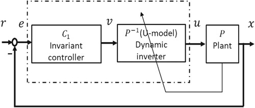
It is noted that the HOFA is a type of model-based (nominal model of $f(\cdot )$ is used for the controller design) approach.

3. Model-free nonlinear-dynamic-coupling inversion/inverter (NDCI)

3.1. Model unknown MIMO plants

Expand the SISO system model (1) into a class of general m-dimensional square MIMO nonlinear dynamic plants as below. (4) $\sum {}_{mimo}:y^{(n)}=F(y^{(0\sim n-1)},u,d)$(4) where $y={\left[\begin{array}{ccc}{y}_1& \cdots & y_m\end{array}\right]}^T\in {\mathsf{R}}^m$ and $u={\left[\begin{array}{ccc}{u}_1& \cdots & u_m\end{array}\right]}^T\in {\mathsf{R}}^m$ are the system output and input vectors, respectively. For the output dynamic expressions, $\begin{array}{rl}{y}^{(n)}& ={\left[\begin{array}{ccc}{y}_1^{(n_1)}& \cdots & y_m^{(n_m)}\end{array}\right]}^T\in {\mathsf{R}}^m,\\ y^{(0\sim n-1)}& ={[y_1^{(0\sim n_1-1)}\cdots y_m^{(0\sim n_m-1)}]}^T\in {\mathsf{R}}^m\end{array}$and $y_i^{(0\sim n_i-1)}=[y_i\cdots y_i^{(n_i-1)}{]}^T\in {\mathsf{R}}^{n_i},\mathrm{\forall }i=1,\dots m$. The function $F={\left[\begin{array}{ccc}{f}_1& \cdots & f_m\end{array}\right]}^T:u\to y$ is a sufficiently differentiable mapping vector from the input space to the output space and $d={\left[\begin{array}{ccc}{d}_1& \cdots & d_m\end{array}\right]}^T\in {\mathsf{R}}^m$ is the external disturbance vector. The MIMO plant description shares, in proper dimension, the same properties as those assumed with the SISO plant (1). This study treats the MIMO plant as total uncertainty, except the dynamic order of each sub-plant is assumed known in the control system design, to develop a new model-free robust decoupling control framework.

To represent the interactions of all the outputs, let $\overline{Y}:=y_1^{(0\sim n_1-1)}\times \cdots \times y_m^{(0\sim n_m-1)}\in {\mathsf{R}}^{{\sum }_{i=1}^{m}i}$. Consequently, plant (4) can be expressed as (5) $\sum {}_{\text{mimo}}:y^{(n)}=F(\overline{Y},u,d)$(5) To represent the couplings/interactions between the plant input vector $u$ and output vector $y$, this study proposes using an I/O coupling matrix function, so that plant (5) can be expressed as (6) $\sum {}_{\text{mimo}}:y^{(n)}=F_y(\overline{Y},d)+U(\overline{Y},u)$(6) where $U(\overline{Y},u)=U(\ast )=U\in {\mathsf{R}}^{mm}$ is defined as the I/O coupling matrix function (I/O-CMF). Consequently, for decoupling control of plant (6), let (7) $\sum {}_{\text{mimo}}:\{\begin{array}{rl}& y^{(n)}=F_y(\overline{Y},d)+U(\overline{Y},u)\\ & U(\overline{Y},u)=Dv\end{array}$(7) where $v={\left[\begin{array}{rlr}{v}_1& \dots & v_m\end{array}\right]}^T\in {\mathsf{R}}^m$ is the virtual controller vector, in which each of the elements is to be designed by SISO control approaches, and $D\in {\mathsf{R}}^{mm}\cap \text{rank}(D)=m$ is the decoupling matrix to be assigned depending if the control matrix function $U(\ast )$ is given or unknown.

3.2. Input/Output (I/O) decoupling

Definition of input-output decoupling (Nijmeijer & van der Schaft, 1990): For plant (4) it is called input-output coupled, by a feasible relabelling of the inputs with the following properties hold.

1. The output $y_i,i\in m$ is invariant with the inputs $u_j,j\ne i,i,j\in m$.

2. The output $y_i,i\in m$ is not invariant with the inputs $u_i,i\in m$.

This section presents model-based and model-free decouplers.

3.2.1. Decoupling with given I/O-CMF – model-based decoupler (U-decoupler)

In the case of $U(\ast )$, the decoupling is a way of solving the systems of equations below (8) $U(\overline{Y},u)-v{|}_{D=I_m}=0\to u:{\mathsf{R}}^{mm}\to {\mathsf{R}}^m$(8) where $u={\left[\begin{array}{ccc}{u}_1& \cdots & u_m\end{array}\right]}^T\in {\mathsf{R}}^m$ is the controller output/plant control input and $v={\left[\begin{array}{ccc}{v}_1& \cdots & v_m\end{array}\right]}^T\in {\mathsf{R}}^m$ is the controller input/virtual control.

Remark 3.1:

Various algorithms for solving systems of nonlinear equations have been effectively applicable (Amiri et al., 2019). In the solution of the systems of nonlinear equations, assume the general fundamental conditions, existence, boundness and Lipschitz continuity, are satisfied. Make it clear, this is not the focus of the study, which merely uses the Matlab function  to obtain the numerical control vector $u$ in simulation demonstrations.

Remark 3.2:

It should be noted that this is a model-based decoupling procedure for the control input vector $u$, even the virtual control vector $v$ is still determined by a model-free design.

3.2.2. Decoupling with unknown I/O-CMF – a model-free decoupler (D-decoupler)

In the case of $U(\ast )$ unknown, to obtain a model-free coupling effect, an assumption is made for the following equality holds. (9) $U(\ast )=Bu+\beta$(9) where $B=\left[\begin{array}{ccc}{b}_{11}& \mathsf{K}& b_{1m}\\ \mathsf{M}& \mathsf{O}& \mathsf{M}\\ b_{m1}& \mathsf{K}& b_{mm}\end{array}\right]\in {\mathsf{R}}^{mm},\text{ rank}(B)=m$ is the coupling gain matrix to reflect the input/output (I/O) interactions and $\beta$ is the residual to $U(\ast )$. $U(\ast )=Bu+\beta$ represents a linear affine control $Bu$ approximation to the nonlinear non-affine I/O-CFM $U(\ast )$.

Accordingly, system (7) can be rewritten as follows. (10) $\sum {}_{mimo}:\{\begin{array}{rl}{y}^{(n)}& =F_y(\overline{Y},d)+U(\overline{Y},u)\\ & =F_y(\overline{Y},d)+Bu+\beta \\ u& =Dv\end{array}$(10) For decoupling, assign the decoupler $D=B^{-1}$ under certain conditions ($\beta \to 0$) in the design. Consequently, there is no need to find the matrix $B$, which alternatively tunes the matrix $D$. Then substituting $Bu=BDv=B{B}^{-1}v=I_{m}v$ into (10) to yield (11) $\sum {}_{mimo}:\{\begin{array}{rl}{y}^{(n)}& =F_y(\overline{Y},d)+Bu+\beta \\ & =F_y(\overline{Y},d)+{I_{m}v|}_{\beta \to 0\cap D=B^{-1}}\\ u& =Dv\end{array}$(11) That is, in effect, the system is decoupled into m isolated sub-control systems in the form of (12) $y_i^{(n_i)}=F(\overline{Y},\beta ,d)+v_i,i\in [1\dots m]$(12)

Theorem 3.1:

The model-free D-decoupler converges to the model-based U-decoupler $Bu\to U(\ast )$ while the residual $\beta \to 0$.

Proof:

Express the residual from (9) as (13) $\beta =U(\ast )-Bu$(13) Assign a Lyapunov function $V=\frac{1}{2}{\beta }^2$ and its derivative accordingly is expressed as (14) $\begin{array}{rl}\dot{V}& =\beta \dot{\beta }=(U(\ast )-Bu)\left(\dot{U}(\ast )\frac{\mathrm{\partial }U(\ast )}{\mathrm{\partial }u}-B\dot{u}\right)\\ & =(U(\ast )-B{D}^{-1}v)\left(\dot{U}(\ast )\frac{\mathrm{\partial }U(\ast )}{\mathrm{\partial }v}-B{D}^{-1}v\right)\end{array}$(14) while $\dot{V}<0$, $\beta \to 0$ from Lyapunov stability condition.

Corollary 3.1:

Matrix $D$ is not unique because the differential inequality $\dot{V}=(U(\ast )-B{D}^{-1}v)(\dot{U}(\ast )\frac{\mathrm{\partial }U(\ast )}{\mathrm{\partial }v}-B{D}^{-1}v\phantom{\frac{\mathrm{\partial }U(\ast )}{\mathrm{\partial }v}})<0$ has multiple solutions.

Remark 3.3:

The Corollary chooses the matrix $D$ more relaxed than the unique choice from solving equality equations. This gives a much stronger robust tuning of the matrix $D$ within a large range of choices.

Remark 3.4:

Compared with the other linear and nonlinear decouplers (Hou et al., 2021; Liu et al., 2019), the new decouplers have several obvious merits, such as (1) does not increase system dynamic order, (2) does not require decoupling interconnections, (3) does not introduce summation elements, (4) does not take up pole/zero cancellation, (5) for D-decoupler, there is no need to estimate/approximate nonlinear nominal models offline and/or online.

The procedure (the rule of thumb) to tune the matrix $D$ is listed with the TITO systems below

1. Always make sure $Rank(D)\in {\mathsf{R}}^m$, that is, $det(D)\ne 0$.

2. Start from setting up $D=diag(D),\mathrm{\forall }{d}_{11}=d_{22}=1$. If a good decoupling effect is observed, this is the case without input/output coupling. The matrix $D$ is determined.

3. Otherwise, set up $D=\left[\begin{array}{cc}\pm d_{11}& \pm d_{12}\\ \pm d_{21}& \pm d_{22}\end{array}\right]$ to start tuning, by trial and error, from $D=\left[\begin{array}{cc}\pm 1_{11}& \pm {0.3}_{12}\\ \pm {0.5}_{21}& \pm 2_{22}\end{array}\right]$. Large absolute values have a high gain effect.

4. As the matrix $D$ is determined in the principle of the Lyapunov differential inequality for its derivative rather than the Lyapunov derivative equality, there are various choices of the matrix to achieve the input/output decoupling effect.

5. From the group of feasible decoupling matrices $D$, select the better fit, for example, regarding the control input with low amplitude and less fluctuation in the steady states.

It should be noted that a systematic procedure to tune the matrix $D$ could be progressively established with more applications.

3.3. Model-free nonlinear dynamic inversion (NDI)

A model-free SMC (MFSMC) has been proposed to achieve the NDI. The MFSMC (Zhu, 2021) has been studied with certain progressions (formulation and demonstration); however, the general MFSMC existing theorem has not been proved. Consider a control vector $u$ specified for MIMO SMC below. (15) $u=\text{smc}\in {\mathsf{R}}^m$(15) where $\text{smc}={\left[\begin{array}{ccc}\text{sm}{\text{c}}_1& \dots & \text{sm}{\text{c}}_m\end{array}\right]}^T\in {\mathsf{R}}^m$.

To design each of the model-free SMCs with an output vector $y_i^{(0\sim n_i-1)}={\left[\begin{array}{cccc}{y}_{i1}& {\dot{y}}_{i1}& \cdots & y_{i1}^{(n_i-1)}\end{array}\right]}^T\in {\mathsf{R}}^{n_i}$, assign the corresponding sliding function and the derivative, which satisfy the Lyapunov asymptotic stability conditions. For determining the equivalent control, consider a set of design criteria below (16) $\begin{array}{rl}{\sigma }_i& ={\mu }_i({\text{e}}_i){|}_{\mathrm{\forall }t\ge 0,||\mu ({\text{e}}_i)||\prec {\delta }_i}:{\mathsf{R}}^{n_i}\to \mathsf{R}\\ {\dot{\sigma }}_i& =u_i={\rho }_i({\sigma }_i){|}_{{\dot{\sigma }}_i{\sigma }_i\prec 0}:{\mathsf{R}}^{n_i+m_i}\to \mathsf{R}\end{array}$(16) where ${\sigma }_i$ and ${\dot{\sigma }}_i$ are the sliding function and the derivative associated with its output, respectively, ${\text{e}}_i=y_i^{(0\sim n_i-1)}-y_{di}^{(0\sim n_i-1)}={\left[\begin{array}{cccc}{\tilde{y}}_i& {\dot{\tilde{y}}}_i& \cdots & {\tilde{y}}_i^{(n_i-1)}\end{array}\right]}^T\in {\mathsf{R}}^{n_i}$ is the output tracking error vector and $y_{di}^{(0\sim n_i-1)}=[\phantom{y_{di}^{(n_i-1)}}{y}_{di}{\dot{y}}_{di}{\cdots y_{di}^{(n_i-1)}]}^T\in {\mathsf{R}}^{n_i}$ is the desired output vector. Accordingly, the sliding function is commonly defined as ${\sigma }_i={\mu }_i({\text{e}}_i)=c_i{\text{e}}_i\in {\mathsf{R}}^{n_i}\to \mathsf{R}$, where ${\sigma }_i=c_i{\text{e}}_i=0$ is a Hurwitz stable polynomial with the properly assigned coefficient vector $c_i$.

Theorem 3.2

(MFSMC existing theorem): For easy formality proof, consider a SISO plant (1) $\sum {}_{\text{SISO}}\text{: }{y}^{(n)}=f(y^{(0\sim n-1)},u,d)$, with a properly assigned sliding function $\sigma$ and its derivative $\dot{\sigma }$. Assign a Lyapunov function $V$ in terms of sliding function $\sigma$with $V(\sigma )=\frac{1}{2}{\sigma }^2\ge 0$, to satisfy Lyapunov asymptotic stability condition, it also requires the derivative of the Lyapunov function $\dot{V}=\dot{\sigma }\sigma \prec 0$. Regarding MFSMC, it has $\mathrm{\exists }u=\rho (\sigma ){|}_{{\dot{\sigma }}_i{\sigma }_i\prec 0}$, under the conditions of (1) $\rho (\sigma ):\{\begin{array}{c}\rho ({\sigma }_1)>\rho ({\sigma }_2),\mathrm{\forall }{\sigma }_1<{\sigma }_2\\ 0,\mathrm{\forall }{\sigma }_1={\sigma }_2\end{array}$ is a monotonically decreasing function, and (2) $|\hat{f}{|}_{max}<|\rho (\sigma )|$, where $|\hat{f}{|}_{max}$ is the bound of plant (1) in the expression of $\sum {}_{\text{SISO}}\text{: }{y}^{(n)}=f(y^{(0\sim n-1)},u,d)=\hat{f}(y^{(0\sim n-1)},u_1,d)+u_1$. With the two conditions, a set of controls $u=\rho (\sigma )$ exist to give rise to the Lyapunov stabilised control systems in terms of $\dot{V}=\{\begin{array}{c}\dot{\sigma }\sigma <0,\mathrm{\forall }\rho (\sigma )\sigma <0\\ 0,\mathrm{\forall }\sigma =0\end{array}$.

Proof:

Let $u=\rho (\sigma )$, for the first condition, to achieve $\dot{V}=\dot{\sigma }\sigma \sim \rho (\sigma )\sigma <0$, it requires (1) $\mathrm{sgn}(u=\rho (\sigma ))=-\mathrm{sgn}(\sigma )$ which is achieved by $u=\rho (\sigma )$ being a decreasing monotone function of $\sigma$ and $\dot{\sigma }=\rho (\sigma )=0,\mathrm{\forall }\sigma =0$ indicates the state vector converged to the origin. For the second condition, (2) let $\sum {}_{SISO}\text{: }{y}^{(n)}=f(y^{(0\sim n-1)},u,d)=\hat{f}(y^{(0\sim n-1)},u_1,d)+u_1$ and $\dot{\sigma }=(y^{(n)}+\dot{\sigma }\mathrm{\setminus }{y}^{(n)})=(f+\dot{\sigma }\mathrm{\setminus }{y}^{(n)}){|}_{f=y^{(n)}}=(\hat{f}+u_1+\dot{\sigma }\mathrm{\setminus }{y}^{(n)}){|}_{u_1=u-\dot{\sigma }\mathrm{\setminus }{y}^{(n)}}=\hat{f}+\rho (\sigma ){|}_{u=\rho (\sigma )}$. As $u=\rho (\sigma )$ is a decreasing monotone function of $\sigma$, to achieve $\dot{V}=\dot{\sigma }\sigma \prec 0$, it requires $|\hat{f}{|}_{max}<|\rho (\sigma )|$, which is still a decreasing monotone function of $\sigma$.

Corollary 3.2:

Rather than just a sole solution from $u=\rho (\sigma ){|}_{\dot{\sigma }=0}$ with model-based SMC, there are various options for selecting $u=\rho (\sigma ){|}_{\dot{\sigma }\sigma \prec 0}$ for MFSMC. Here a few examples with both switching control $u_{sw}$ and equivalent control $u_{eq}$ are picked up (Zhu, 2023).

Proportional (P) control (17) $u=\{\begin{array}{cc}{u}_{sw}=-k_g\mathrm{sgn}(\sigma )& \mathrm{\forall }|\sigma |>\delta \\ u_{eq}=\rho (\sigma )=-k_l\sigma & \mathrm{\forall }|\sigma |\le \delta \end{array}$(17) where $|\hat{f}{|}_{max}<k_g<|k_u{|}_{max},\mathrm{\forall }{u}_{sw}$ and $|\hat{f}{|}_{max}<k_l<|k_u{|}_{max},\mathrm{\forall }{u}_{eq}$, where $|\hat{f}{|}_{max}$ is the plant bound and $|k_u{|}_{max}$ is the controller saturation bound. Consequently, it achieves $\underset{t\to \mathrm{\infty }}{lim}\sigma (\tilde{\mathrm{y}})\to 0:\to \underset{t\to \mathrm{\infty }}{lim}\tilde{\mathrm{y}}=\text{y}-{\text{y}}_d\to 0,\underset{t\to \mathrm{\infty }}{lim}{\text{y}}^{-1}{\text{y}}_d\to I_n$.

Proportional and integral (PI) control (18) $u=\{\begin{array}{cc}{u}_{sw}=-k_g\mathrm{sgn}(\sigma )& \mathrm{\forall }|\sigma |>\delta \\ u_{eq}=\rho (\sigma )=-k_p\sigma -k_i\int \sigma & \mathrm{\forall }|\sigma |\le \delta \end{array}$(18) Similarly, the PI control can achieve the Lyapunov stability conditions $V=\frac{1}{2}{\sigma }^2>0\cap \dot{V}=\dot{\sigma }\sigma <0$ with the properly assigned gains $k_g,k_p,k_i$ to make the controller $u=\rho (\sigma )$ a decreasing monotone function of $\sigma$.

Continuous control with monotone bounded hyperbolic tangent function (19) $u=\rho (\sigma )=-k_h\tanh (k_0\sigma )\sigma$(19) where the controller parameters $k_g,k_p,k_i$ have properly tuned the controller $u=\rho (\sigma )$ a decreasing monotone function of $\sigma$ is to satisfy the Lyapunov stability conditions $V=\frac{1}{2}{\sigma }^2>0\cap \dot{V}=\dot{\sigma }\sigma <0$

Remark 3.5:

The gains in the above controllers are specified to remove the sign impact from the plants to achieve $\dot{\sigma }\sigma =\rho (\sigma )\sigma \prec 0$. Consequently, a large range of gain options to satisfy the Lyapunov asymptotic stabilisation conditions, which relax the choices of the gain tunings – increase the robustness.

Remark 3.6:

The generalised MFSMC covers (1) asymptotical stabilisation by assigning the sliding function with Hurwitz stable polynomials, (2) finite-time stabilisation by assigning the sliding function with fractional stable polynomials and (3) both model-based design and model-free design of the controller by assigning the SF derivative $\dot{\sigma }=\rho (u)=0$ or $\dot{\sigma }=u\rho (\sigma )<0$ (Zhu, 2021).

Corollary 3.3

For the dynamic inversion $C_{NDI}({\hat{P}}^{-1},P)\stackrel{asymp}{⟶}{I}_n$ in all the cases above, because $\underset{t\to \mathrm{\infty }}{lim}\sigma (\tilde{\mathrm{y}})\to 0:\to \underset{t\to \mathrm{\infty }}{lim}\tilde{\mathrm{y}}=\text{y}-{\text{y}}_d\to 0$ implies $\text{y = }{I}_n{\text{y}}_d$, that is, $C_{NDI}({\hat{P}}^{-1},P)\stackrel{asymp}{⟶}\text{y}=I_n{\text{y}}_d\to \text{y}={\text{y}}_d\to I_n$

Property 3.1:

Consider a dynamic model $f=|\hat{f}|+|\epsilon |$ (could be nonlinear and/or time-varying) (Slotine & Li, 1991), where $\hat{f}$ is the nominal model used as a basis for model-based control system design and $\epsilon$ is the uncertainty or model error subject to $f$. The percentage of robustness control is defined here as $R=\frac{|\epsilon |}{|\hat{f}|+|\epsilon |}(\mathrm{\%})$. For the model-free approach, $R=\frac{|\hat{f}|+|\epsilon |}{|\hat{f}|+|\epsilon |}=100(\mathrm{\%})$, accordingly called total/full robustness control. Obviously, for those model-based approaches, the robustness percentage is less than such model-free approaches.

3.4. Procedure for achieving NDCI

In summary, the NDCI procedure within the inner loop is outlined below.

1. Take the MIMO plant as a total uncertainty, except assume the dynamic order of each sub-output known in the SMC design.

2. Separate independently design the model-free D-decoupler by assigning the decoupling matrix $D$.

3. Separate independently design the nonlinear dynamic inverter by model-free SMC (SF ${\sigma }_i={\mu }_i({\tilde{\mathrm{y}}}_i)$, sliding band thickness ${\delta }_i$, and switching/equivalent controls $v_{swi}$/$v_{eqi}$.

4. While the output dynamic vector for feedback control is not available/measurable, an observer, such as an extended state observer (ESO) needs to be introduced to estimate the vector.

5. The desired output vectors $y_{di}$ are specified/provided by the outer loop in the U-control framework.

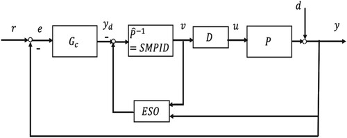
4. MIMO model-free decoupling U-control (MFDUC) platform

As shown in Figure 3, the MIMO U-control platform is functionally expressed as (20) $\begin{array}{rl}& {\mathrm{\Sigma }}_{\text{Umimo}}:(F,C(C_{IV},{\hat{P}}^{-1},D),P)\\ & \iff (F,C_{IV},C_{NDCI}({\hat{P}}^{-1},D,P)\in I_m)\\ & \iff (F,C_{IV},I_m)\end{array}$(20) Below is the description of the two loops designed.

1. Trimming plant in the inner loop – robust stability: NDI for SISO systems has been explained in Section 2. As the decoupling control design still uses the SISO technique to design the MIMO control systems, (1) the SISO NDI remains in its feasibility and (2) the decoupling proposed in the study is independently achieved from NDI. Subsequently, it gives NDCI in the form of $C_{NDCI}({\hat{P}}^{-1},D,P)\iff (C_{NDI},D)\in I_m$, in which the formulations have been presented in the above sections. It is noted that there are two decouplers developed in the study, model-based $U$-decoupler and model-free $D$-decoupler.

2. Assigning system performance – dynamics/steady states: The outer loop controller $C_{IV}$ design includes

   1. Assign I/O paring linear dynamic performance $g=\text{diag}\left[\begin{array}{ccc}{g}_{11}({\zeta }_1,{\omega }_{n1})& \dots & g_{mm}({\zeta }_m,{\omega }_{nm})\end{array}\right]$, where $g$ is for the decoupled O/I Laplace transfer function (dynamic gain matrix) with specified damping ratio and undamped natural frequency ($\begin{array}{cc}{\zeta }_i,& {\omega }_{ni}\end{array}$), in which the asymptotic stability means all the roots lying in the open left half-plane on the complex plane and the steady-state error $\underset{t\to \mathrm{\infty }}{lim}(r_i(t)-y_i(t))=\underset{t\to \mathrm{\infty }}{lim}{e}_i(t)=0$ to a given level reference vector $r=\text{diag}\left[\begin{array}{ccc}{r}_1& \dots & r_m\end{array}\right]$.

   2. Determine the invariant controller $C_{IV}$, converting the system performance into a closed-loop implementation by taking the dynamic inverse of the performance transfer function as $C_{VI}=g(I_m-g{)}^{-1}$.

   3. Provide reference vector $y_d={\left[\begin{array}{ccc}{y}_{d1}& \dots & y_{dm}\end{array}\right]}^T\in {\mathsf{R}}^{n_1\times \cdots \times n_m}$ for each I/O paring path, $y_i={\left[\begin{array}{cccc}{y}_{i1}& {\dot{y}}_{i1}& \cdots & y_{i1}^{(n_i-1)}\end{array}\right]}^T\in {\mathsf{R}}^{n_i}$ in the inner loop NDCI, configure the invariant control $C_{IV}$ in state space realisation to provide the output derivative reference vector automatically.

Figure 3. Model-free MIMO U-control platform.

5. Case studies

The simulation considers a two-input and two-output (TITO) plant below. (21) $P_{2x2}:\{\begin{array}{rl}& {\ddot{y}}_1+y_2{\dot{y}}_1+u_2{\dot{y}}_2+0.6y_1-\sin (u_1)\\ & -2u_2-u_1^3=0\\ & {\ddot{y}}_2-1.5(1-y_1^2){\dot{y}}_2+y_1-2u_1+u_2^3=0\end{array}$(21) The external level disturbances, a typical non-vanishing disturbance, are assigned with $d_1(t)=1d_2(t)=0.2$ added at the corresponding outputs, respectively.

Inspect plant (21), the first line of the plant is a nonlinear nonaffine dynamic and the second line is an expanded Van der Pol equation with nonlinear control input, the interconnect outputs and the I/O couplings are apparently observed in the sub-plants.

This case study is set up for testing the decoupling control implemented within the MIMO U-control framework. The analytically designed NDCI and invariant control need to be demonstrated numerically if they are consistent with the expected results. For a set of given references (${\left[\begin{array}{cc}{r}_1(t)=4& r_2(t)=\sin (t)\end{array}\right]}^T,\mathrm{\forall }t\ge 0$) and a black-box plant with the given dynamic orders of each sub-plant, plus assuming the output derivatives are available for the control system designs, otherwise output derivative observers, revised from the state observers, can be taken in to estimate the derivative vectors.

The decoupling control objective is described as I/O paring performance, decoupled output responses with specified damping ratio and undamped natural frequency ($\begin{array}{cc}{\zeta }_i,& {\omega }_{ni}\end{array}$) and the steady-state error to level references $\underset{t\to \mathrm{\infty }}{lim}(r_i(t)-y_i(t))=\underset{t\to \mathrm{\infty }}{lim}{e}_i(t)=0,i=1,2$.

5.1. Control system design

Regarding Figure 3, as the output derivative vectors are available, there is no need to use observers. The control system design procedure includes the following separate sections.

1. Design NDI through model-free SMC: Specify the sliding function with ${\sigma }_i=20(y_i-y_{di})+({\dot{y}}_i-{\dot{y}}_{di})=20e_i+{\dot{e}}_i,i=1,2$. Set up the sliding mode band thickness ${\delta }_i=1,i=1,2$. Assign the SM controllers with $v_i=\{\begin{array}{cc}-k_{gi}\mathrm{sgn}({\sigma }_i)& \mathrm{\forall }{u}_{swi}\\ -k_{pi}{\sigma }_i& \mathrm{\forall }{u}_{eqi}\end{array},i=1,2$ and $\left[\begin{array}{cc}{k}_{g1}=k_{g2}=-5& k_{p1}=k_{p2}=-5\end{array}\right]$ (tuned by trial and error).

2. Design decouplers: This includes the design of the two types of decouplers, model-based (U-decoupler) and model-free (D-decoupler).

For the model-based U-decoupler, the coupling control matrix function is extracted from the plant (21) and the control input vector is determined by solving the following nonlinear systems of equations. (22) $U:\{\begin{array}{c}-u_2{\dot{y}}_2+\sin (u_1)+2u_2+u_1^3=v_1\\ 2u_1-u_2^3=v_2\end{array}$(22) For the mode-free D-decoupler, tune the decoupling gain matrix $D=\left[\begin{array}{cc}1& 2\\ 1& -3\end{array}\right]$ with trial-and-error tests. Because of the multiple choice of the matrix $D$, the other choices of the D-decoupler also have been tested in the simulation.

1. Design invariant controllers: For the whole closed-loop control system Laplace transfer function matrix $Y(s)/R(s)=G(s)$, assign the I/O paring linear dynamic performance in terms of a diagonal matrix $G=\text{diag}\left[\begin{array}{cc}{g}_{11}({\zeta }_1,{\omega }_{n1})& g_{22}({\zeta }_2,{\omega }_{n2})\end{array}\right]$ and specify the two diagonal transfer functions as (23) $\begin{array}{rl}\frac{Y_i}{R_i}& =g_{ii}=\frac{C_{IVi}\text{SM}{\text{C}}_i({\hat{P}}^{-1}\ast P)}{1+C_{IVi}}=\frac{C_{IVi}}{1+C_{IVi}}\\ & =\frac{{\omega }_{ni}^2}{s^2+2{\zeta }_i{\omega }_{ni}s+{\omega }_{ni}^2},\{\begin{array}{cc}{\zeta }_1=0.7& {\omega }_{n1}=1\\ {\zeta }_2=1& {\omega }_{n2}=1\end{array}\end{array}$(23)

Therefore, the two controllers are designed by taking the inversion of the system’s closed-loop transfer function $G_{ii}$, which are expressed as (24) $\begin{array}{rl}{C}_{IVi}& =\frac{G_{ii}}{1-G_{ii}}=\frac{{\omega }_{ni}^2}{s(s+2{\zeta }_i{\omega }_{ni}s)},\\ & \begin{array}{cc}\{\begin{array}{c}{\zeta }_1=0.7\\ {\zeta }_2=1\end{array}& \begin{array}{c}{\omega }_{n1}=1\\ {\omega }_{n2}=1\end{array}\end{array}\end{array}$(24)

The invariant controllers also provide desired reference vectors for the SMCs in the inner loop. Accordingly, from (24) these desired output derivative vectors are formed $y_{di}^{(0\sim 1)}={\left[\begin{array}{cc}{y}_{di}& {\dot{y}}_{di}\end{array}\right]}^T={\left[\begin{array}{cc}\frac{1}{s}\frac{{\omega }_n^2}{s+2\zeta {\omega }_n}& \frac{{\omega }_n^2}{s+2\zeta {\omega }_n}\end{array}\right]}^T$.

It should be noted that throughout the simulation process, the plan model was not used as a reference for designing the controller except for the mode-based U-decoupler. That is, the plant is treated completely as an uncertainty, only the input/output are available and the dynamic order of the plant is assumed known in advance.

5.2. Simulation tests and discussions

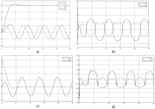
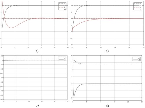
Matlab/Simulink is used to conduct the computational experiments. Figure 4 shows the control system response using I/O-CCFM $U(\ast )$ decoupler and Figure 5 is generated with a model-free decoupler $D$. To test the dynamic and coupling variation to the system response, set $(1+\mathrm{\Delta })y_2$ ($\mathrm{\Delta }=\left[\begin{array}{cc}-0.4& 0.4\end{array}\right]$ is the variation, taking up 40% deviation range) as $y_2$ is interacted with both sub-plant and associated with control $u_2$. Figures 6 and 7 show the responses from using decouplers $U$ and $D$, respectively. Inspect the plots and draw the following observations/discussions.

1. The fundamental ideas, in terms of two dynamic inversions (NDI and invariant controller) and one static inversion (matrix inversion/D-decoupler and solution of set equation/U-decoupler) through model-free SMC, control system specification and decoupling within the MIMO U-control framework, are consistent with the analytical results presented in the study. Inspection of all figures a, the paring performance with the reference and output response is reasonably reflecting the design specifications. It is noted that the second sub-system output response to the sinusoidal (with a frequency of 1/rad) reference has ${90}^{\circ }$ phase delay, this is because the frequency response $g_2(\omega =1)={\frac{1}{{(j\omega )}^2+j2\omega +1}|}_{\omega =1}=\frac{1}{-1+j2+1}=\frac{1}{j2}=0.5\mathrm{\angle }-{90}^{\circ }$, a forward gain of 2 has been added to compensate for the amplitude reduction in the simulation.

2. For the decoupling controller output $u$ vector, as shown in Figures b, both U and D-decouplers have a similar amplitude range $u_i\sim \pm 3,i=1,2$. However, the U-decoupler produces fast oscillation in the starting phase and a longer time (solving the nonlinear system equations) compared with the D-decoupler in the simulations. With the successful control effect, the coupling matrix B can be obtained by $D=B^{-1}=\left[\begin{array}{cc}1& 2\\ 1& -3\end{array}\right]$, which could be a useful reference for understanding the plant and maintaining/revising the control system in the future. In addition, to test the multiple choice matrix $D$, the simulation selected $D=\left[\begin{array}{cc}1& 5\\ 1& -3\end{array}\right]$, $D=\left[\begin{array}{cc}1& 0\\ 1& -1\end{array}\right]$, and $D=\left[\begin{array}{cc}1& 0\\ 1& -5\end{array}\right]$ All these showed the well-decoupled control results and robustness in assigning the D-decouplers.

3. For the error of each subsystem, the difference between the reference and output, as shown in Figure c, the errors to level references are, as expected, well asymptotically converged to zero. For the errors to sinusoidal references are, as expected, the same frequency but are obvious due to the phase lag. A merit point observed from the plots is that the nonlinear control system does not induce harmonics, this conforms once again to the achievement of NDI to make the whole system operate by the linear dynamics specified.

4. NDI by SMC significantly facilitates such insight and formulations, dealing with chattering effects at the controller output, as the equivalent controller output in model-free SMC is formulated by $\dot{\sigma }\sigma \prec 0$ (this is asymptotic Lyapunov stability) rather than most popularly model-based SMC with $\dot{\sigma }=0$ (only Lyapunov stability) which is one of the sources inducing chattering. With the MFSMC, the sliding band thickness is relatively relaxed without losing steady-state accuracy as the sliding function and its derivative are asymptotically converged to zero. For sliding function (SF), as shown in figure d, the U-decoupler clearly shows the two SFs separated and the D-decoupler has mixed up the two SFs within the sliding mode bands.

5. To test the dynamic and coupling variation to the system response, particularly for the decoupling effect. In the case of both dynamic interaction and I/O coupling from $y_2$, conducted a series of tests of $(1+\mathrm{\Delta })y_2$ ($\mathrm{\Delta }=\left[\begin{array}{cc}-0.4& 0.4\end{array}\right]$, a 40% deviation range). Figures 6 and 7 show the U decoupling and D decoupling control with the test of $(1+0.4)y_2$ respectively. As shown in Figure 6, the U-decoupler still enables the system to track level reference properly, but not the sinusoidal reference in shape, amplitude and phase due to the inaccurate root solutions. The D-decoupler has no such problems as it takes such variations as uncertainties dealt with NDI.

6. While the plant model is completely unknown, the designed control system has a very simple tuning of process in selecting SMC and D-decoupler parameters which have a relatively wide range of choices while keeping almost the same specified performances. For example, the SM controllers with $u_i=\{\begin{array}{cc}-k_{gi}\mathrm{sgn}({\sigma }_i)& \mathrm{\forall }{u}_{swi}\\ -k_{pi}{\sigma }_i& \mathrm{\forall }{u}_{eqi}\end{array},i=1,2$ and $\left[\begin{array}{cc}{k}_{g1}=k_{g2}=-5& k_{p1}=k_{p2}=-5\end{array}\right]$ were tuned by trial and error, they have a large range of selections to achieve the NDI in terms of robust stabilisation instead of delicate transient response specification (to be achieved by the external loop) similar to the D-decoupler. What was selected have made the smallest control amplitude ranges within the tested set of parameters. Such U-control to relocate control tasks (robust stabilisation and decoupling in the inner loop and control system performance specification in the external loop) separately independently has the potential for industrial co-design, particularly for emerging systems, such as unmanned aerial vehicles (UAV).

7. Regarding the robustness against model internal uncertainty, the control system designed has taken the plant as a whole uncertainty $R=\frac{|\hat{f}|+|\epsilon |}{|\hat{f}|+|\epsilon |}=100(\mathrm{\%})$, and the plots confirm the expected outcomes.

8. The contents presented analytically and validated computationally in the study have followed a route from complexity (problems) to simplicity (analysis and solutions). The derived and simulated are consistent and basically feasible for those with reasonably good control system knowledge to use/expand for their ad hoc research and development. In some sense, this study could be treated as a user manual.

Figure 4. U decoupling control system responses. (a) Output response $y(t)$, (b) Control $u(t)$, (c) Error $e(t)=r(t)-y(t)$, (d) Sliding mode function $\sigma (t)$.

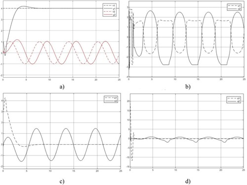
Figure 5. D decoupling control system responses. (a) Output response $y(t)$, (b) Control $u(t)$, (c) Error $e(t)=r(t)-y(t)$, (d) Sliding mode function $\sigma (t)$.

Figure 6. U decoupling control system responses with $(1+\mathrm{\Delta })y_2=(1+0.4)y_2$. (a) Output response $y(t)$, (b) Control $u(t)$, (c) Error $e(t)=r(t)-y(t)$, (d) Sliding mode function $\sigma (t)$.

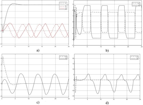
Figure 7. D decoupling control system responses with $(1+\mathrm{\Delta })y_2=(1+0.4)y_2$. (a) Output response $y(t)$, (b) Control $u(t)$, (c) Error $e(t)=r(t)-y(t)$, (d) Sliding mode function $\sigma (t)$.

5.3. Comparative simulation demonstrations

This section compares a commonly used dynamic decoupling control (DDC) approach (Bhattacharyya & Keel, 2022 Cai et al., 2008;) with the new approach MFDUC (with the D decoupler) for a general TITO first-order linear dynamic plant. Figure 8 shows the dynamic decoupling control system and the coupling plant is tested with both decoupling control schemes. The desired closed-loop transfer function is specified by, both decoupling control systems (25) $G(s)=\left[\begin{array}{cc}{\displaystyle \frac{1}{s+1}}& 0\\ 0& {\displaystyle \frac{1}{3s+1}}\end{array}\right]$(25) The reference vector is assigned with ${\left[\begin{array}{cc}{r}_1(t)=4& r_2(t)=2\end{array}\right]}^T,\mathrm{\forall }t\ge 0$. The two control system designs are briefed below.

1. For the DDC, the controllers are expressed by (26) $\begin{array}{rl}{G}_c(s)& =\left[\begin{array}{cc}{G}_{c11}(s)& G_{c12}(s)\\ G_{c21}(s)& G_{c22}(s)\end{array}\right]\\ & =\left[\begin{array}{cc}{\displaystyle \frac{2s+1}{s}}& 0\\ -{\displaystyle \frac{(s+1)(2s+1)}{s}}& {\displaystyle \frac{s+1}{3s}}\end{array}\right]\end{array}$(26)

2. For the MFDUC, keep the SMC the same as used in the first case study, the rest of the work is to tune the D-decoupler, which $D=\left[\begin{array}{cc}10& 3\\ -1& 9\end{array}\right]$ is selected from large feasible decoupling control options.

Figure 8. Dynamic decoupling control.

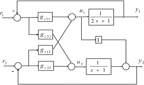
Figure 9 shows the comparisons of the model-matched DDC against the MFDUC. Large initial control inputs ${\left[\begin{array}{cc}{u}_1(0)=8& r_2(0)=-814\end{array}\right]}^T$ are observed from the DDC and the final control inputs are $[u_1(25)=4{r_2(25)=-2.23]}^T$. For the MFDUC, the initial control inputs ${\left[\begin{array}{cc}{u}_1(0)=0& r_2(0)=0\end{array}\right]}^T$ are observed and the final control inputs are ${\left[\begin{array}{cc}{u}_1(25)=3.99& r_2(25)=-10.00\end{array}\right]}^T$.

Figure 9. DDC and MFDUC control systems. (a) Output response $y(t)$ – DDC, (b) Control $u(t)$ – DDC, (c) Output response $y(t)$ – MFDUC, (d) Control $u(t)$ – MFDUC.

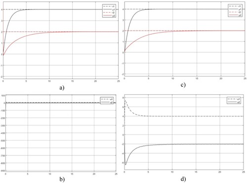
Figure 10 shows the comparisons of the model mismatched DDC which the second sub-transfer function takes $\frac{1}{3s+1}$ in simulation and the nominal model of $\frac{1}{s+1}$ in the design against the MFDUC with the same D-coupler $D=\left[\begin{array}{cc}10& 3\\ -1& 9\end{array}\right]$. Inspect Figure 10, for the DDC large initial control inputs $[u_1(0)=8r_2(0){=-814]}^T$ are observed and the final control inputs are ${\left[\begin{array}{cc}{u}_1(25)=4& r_2(25)=-2.23\end{array}\right]}^T$. For the MFDUC, the initial control inputs ${\left[\begin{array}{cc}{u}_1(0)=0& r_2(0)=0\end{array}\right]}^T$ are observed and the final control inputs are ${\left[\begin{array}{cc}{u}_1(25)=3.99& r_2(25)=-10.00\end{array}\right]}^T$. Obviously, DDC has large dynamic variation in the transient phase, but the MFDUC robustly keeps the response the same as in Figure 9 except the control input vector is accordingly adjusted.

Figure 10. DDC and MFDUC control systems with plant parameter variation. (a) Output response $y(t)$ – DDC, (b) Control $u(t)$ – DDC, (c) Output response $y(t)$ – MFDUC, (d) Control $u(t)$ – MFDUC.

In summary, this comparative study consistently confirms the validity tested with the first case study.

6. Conclusions

Regarding insight/concept for developing new robust control system design approaches, this study takes total uncertain systems (model-free, no need for online model estimation), contrast to nominal model-based uncertain systems (still mode-based), into analysis and design.

To the author’s best knowledge, this is the first study to take MIMO nonlinear nonaffine plants as whole uncertainty to design model-free decoupling control. The study has proposed three types of separate inversions within the U-control framework to achieve its aim in terms of model-free robust decoupling control of multivariable systems. The three inversions are (1) model-free nonlinear dynamic inversion to trim the plant into an identity matrix, which is implemented by a general model-free SMC; (2) static decoupling to cancel the I/O coupling effects, which is implemented by system I/O equations solution (U-decoupler) or a matrix inversion formulation (D-decoupler); (3) whole control system performance inversion for determining the invariant controller for the output control, and simultaneously to provide the desire state vector for the inner loop control.

The presented method could be expanded to provide solutions for the other related issues in MIMO control system design, such as under-actuated control and over-actuated control. In merits, (1) the model-free control methodology has roots in bionics and human heuristic behaviour, which effectively uses the error and the error derivatives in conjunction with SMC. This merit is comparable with mode-free adaptive control which still needs online model updating with the measured errors and the model variables, and the other data-driven learning control approaches in need of online model estimation. (2) The U-control configuration represents a fundamental insight – the control system design is a backward procedure to invert the system with prescribed requests, U-control takes an inverting procedure with two dynamic inversions and one static inversion from [ABC]^∧-1 to [A]^∧-1*[B]^∧-1*[C]^∧-1 = [B]^∧-1*[C]^∧-1*[A]^∧-1 = *** (in any order of the three inversions), which makes the whole control system design separately independently possible and could provide a co-design platform for the effective and speedy design of plant/process and the control independently. (3) The approach is not against model-based methods, in general, it supplements the methods with the whole spectrum from model-based to mode-free. Hopefully, these insights could be supplementary references for the other control approaches in strategic methodology development. Further studies from the current results could be those topics on control of time-delayed multivariable systems, MIMO systems with hard (noncontinuous) nonlinearity and bench test applications.

Acknowledgements

The authors would like to express their gratitude to the editors and the anonymous reviewers for their promotional comments and constructive suggestions regarding the revision of the paper.

Disclosure statement

No potential conflict of interest was reported by the author(s).

Data availability statement

The datasets used and/or analysed during the current study are available from the corresponding author upon reasonable request.

Additional information

Notes on contributors

Quanmin Zhu

Quanmin Zhu is Professor in control systems at the School of Engineering, University of the West of England, Bristol, UK. He obtained his MSc in Harbin Institute of Technology, China in 1983, PhD in Faculty of Engineering, University of Warwick, UK in 1989, and worked a as postdoctoral research associate at the Department of automatic control and systems engineering, University of Sheffield, UK between 1989-2994. His main research interest is in nonlinear system modelling, identification, and control. He has published over 300 papers on these topics, edited various books with Springer, Elsevier, and the other publishers, and provided consultancy to various industries. Currently Professor Zhu is acting as Editor of Elsevier book series of Emerging Methodologies and Applications in Modelling, Identification and Control.

Ruobing Li

Ruobing Li is just completed his PhD at the University of the West England, UK. His main research is in U-control based control system design, simulation, and applications.

Jianhua Zhang

Jianhua Zhang is Associate Professor at School of Information and Control Engineering, Qingdao University of Technology, China. His main research interest is in control math, nonlinear dynamic system control and simulation.

References

- Amiri, A., Cordero, A., Darvishi, M. T., & Torregrosa, J. R. (2019). A fast algorithm to solve systems of nonlinear equations. Journal of Computational and Applied Mathematics, 354, 242–258. https://doi.org/10.1016/j.cam.2018.03.048
- Arkun, Y., Manousiouthakis, B., & Palazoglu, A. (1984). Robustness analysis of process control systems. A case study of decoupling control in distillation. Industrial & Engineering Chemistry Process Design and Development, 23(1), 93–101. https://doi.org/10.1021/i200024a016
- Bhattacharyya, S., & Keel, L. (2022). Linear multivariable control systems. Cambridge University Press. https://doi.org/10.1017/9781108891561
- Cai, W. J., Ni, W., He, M. J., & Ni, C. Y. (2008). Normalized decoupling —A new approach for MIMO process control system design. Industrial & Engineering Chemistry Research, 47(19), 7347–7356. https://doi.org/10.1021/ie8006165
- Celentano, L., Basin, M. V., & Chadli, M. (2020). Robust tracking design for uncertain MIMO systems using proportional–integral controller of order v. Asian Journal of Control, 23(5), 2042–2063. https://doi.org/10.1002/asjc.2405
- Dai, X., He, D., Zhang, X., & Zhang, T. (2001). MIMO system invertibility and decoupling control strategies based on ANN αth-order inversion. IEE Proceedings - Control Theory and Applications, 148(2), 125–136. https://doi.org/10.1049/ip-cta:20010283
- Duan, G. R. (2021). High-order fully actuated system approaches: Part I. Models and basic procedure. International Journal of Systems Science, 52(2), 422–435. https://doi.org/10.1080/00207721.2020.1829167
- Dumont, G. A. (2021). Decoupling control of MIMO systems. (UBC EECE) EECE 460. University of British Columbic.
- Guo, B. Z., & Zhao, Z. L. (2011). On the convergence of an extended state observer for nonlinear systems with uncertainty. Systems & Control Letters, 60(6), 420–430. https://doi.org/10.1016/j.sysconle.2011.03.008
- Hou, M. D., Wang, Y. S., & Yaozhen Han, Y. Z. (2021). Data-driven discrete terminal sliding mode decoupling control method with prescribed performance. Journal of the Franklin Institute, 358(13), 6612–6633. https://doi.org/10.1016/j.jfranklin.2021.06.025
- Huang, H. P., Roan, M. L., & Jeng, J. C. (2002). On-line adaptive tuning for PID controllers. IEE Proceedings - Control Theory and Applications, 149(1), 60–67. https://doi.org/10.1049/ip-cta:20020099
- Hussain, N. A. A., Ali, S. S. A., Ovinis, M., Arshad, M., & Al-saggaf, U. M. (2020). Underactuated coupled nonlinear adaptive control synthesis using U-model for multivariable unmanned marine robotics. IEEE Access, 1851–1965. https://doi.org/10.1109/ACCESS.2019.2961700
- Isidori, A. (2014). Nonlinear control systems. Springer.
- Kang, W., Krener, A. J., Xiao, M. Q., & Xu, L. (2013). A survey of observers for nonlinear dynamical systems. In S. Park, & L. Xu (Eds.), Data assimilation for atmospheric, oceanic and hydrologic applications (Vol. II). Springer. https://doi.org/10.1007/978-3-642-35088-7_1
- Li, R. B., Zhu, Q. M., Kiely, J., & Zhang, W. C. (2020). Algorithms for U-model-based dynamic inversion (UM-dynamic inversion) for continuous time control systems. Complexity, 2020, Article ID 3640210. https://doi.org/10.1155/2020/3640210
- Li, R. B., Zhu, Q. M., Nemati, H., Yue, X. C., & Narayan, P. (2022). Trajectory tracking of a quadrotor using extend state observer based U-model enhanced double sliding mode control. Journal of the Franklin Institute.
- Liu, L., Tian, S., Xue, D., Zhang, T., Chen, Y. Q., & Zhang, S. (2019). A review of industrial MIMO decoupling control. International Journal of Control, Automation and Systems, 17(5), 1246–1254. https://doi.org/10.1007/s12555-018-0367-4
- Mao, J. F., Wu, G. Q., Wu, A. H., & Zhang, X. D. (2011). Nonlinear decoupling sliding mode control of permanent magnet linear synchronous motor based on α-th order inverse system method. Procedia Engineering, 15, 561–567. https://doi.org/10.1016/j.proeng.2011.08.106
- Nijmeijer, H., & Respondek, W. (1988). Dynamic input-output decoupling of nonlinear control systems. IEEE Transactions on Automatic Control, 33(11), 1065–1070. https://doi.org/10.1109/9.14420
- Nijmeijer, H., & van der Schaft, A. (1990). The input-output decoupling problem. In Nonlinear dynamical control systems. Springer. https://doi.org/10.1007/978-1-4757-2101-0_8
- Novara, C., & Milanese, M. (2019). Control of MIMO nonlinear systems: A data-driven model inversion approach. Automatica, 101, 417–430. https://doi.org/10.1016/j.automatica.2018.12.026
- Pandey, S. K., Dey, J., & Banerjee, S. (2021). Generalized discrete decoupling and control of MIMO systems. Asian Journal of Control, 24, 1–19. https://doi.org/10.1002/asjc.2716
- Price, C. R., & Rasmussen, B. P. (2017). Decoupling of MIMO systems using cascaded control architectures with application for HVAC systems. American Control Conference (ACC), 2907–2912. https://doi.org/10.23919/ACC.2017.7963392
- Rodrigues, D., & Mesbah, A. (2021). Multivariable control based on incomplete models via feedback linearization and continuous-time derivative estimation. International Journal of Robust and Nonlinear Control, 31(18), 9193–9230. https://doi.org/10.1002/rnc.5762
- Slotine, J. J. E., & Li, W. P. (1991). Applied nonlinear control. Prentice Hall.
- Wang, Q. G., Ye, Z., Cai, W. J., & Hang, C. C. (2008). PID control for multivariable processes. Springer.
- Wang, W., Hou, Z., & Jin, S. (2009). Model-free indirect adaptive decoupling control for nonlinear discrete-time MIMO systems. Proceedings of the 48 h IEEE Conference on Decision and Control (CDC) (pp. 7663–7668). https://doi.org/10.1109/CDC.2009.5400164.
- Wu, B., Wu, J., Zhang, J., Tang, G., & Zhao, Z. (2022). Adaptive neural control of a 2DOF helicopter with input saturation and time-varying output constraint. Actuators, 11(11), 336. https://doi.org/10.3390/act11110336
- Ye, H., & Song, Y. (2022). Prescribed-time tracking control of MIMO nonlinear systems under non-vanishing uncertainties. IEEE Transactions on Automatic Control. https://doi.org/10.1109/TAC.2022.3194100
- Zhang, Q., & Wang, A. (2017). Decoupling control in statistical sense: Minimised mutual information algorithm. International Journal of Advanced Mechatronic Systems, 7(2), 61–70. https://doi.org/10.1504/IJAMECHS.2016.082625
- Zhang, Q., & Zhou, Y. (2022). Recent advances in non-gaussian stochastic systems control theory and its applications. International Journal of Network Dynamics and Intelligence, 1(1), 111–119. https://doi.org/10.53941/ijndi0101010
- Zhang, W. C., Zhu, Q. M., Mobayen, S., Yan, H., Qiu, J., & Narayan, P. (2020). U-Model and U-control methodology for nonlinear dynamic systems. Complexity, ID1050254. https://doi.org/10.1155/2020/1050254
- Zhao, J., Han, F., Wang, Y., Zhang, X., Zhang, G., & Du, G. (2021). Decoupling control of multi-DOF supporting system of MLDSB. Applied Sciences, 11(16), 7239. https://doi.org/10.3390/app11167239
- Zhou, F., Shen, Y., & Li, L. (2023). Adaptive output feedback controller of resisting large measurement noises for MIMO nonlinear systems. International Journal of Systems Science, 54(2), 264–282. https://doi.org/10.1080/00207721.2022.2113175
- Zhu, H. Q., & Wang, S. S. (2020). Decoupling control based on linear/non-linear active disturbance rejection switching for three-degree-of-freedom six-pole active magnetic bearing. IET Electric Power Applications, 14(10), 1818–1872. https://doi.org/10.1049/iet-epa.2019.0448
- Zhu, Q. M. (2021). Complete model-free sliding mode control (CMFSMC). Scientific Reports, 11(1), 22565. https://doi.org/10.1038/s41598-021-01871-6
- Zhu, Q. M. (2023). Model-free sliding mode enhanced proportional, integral, and derivative (SMPID) control. Axioms, 12(8), 721. https://doi.org/10.3390/axioms12080721
- Zhu, Q. M., & Guo, L. (2002). A pole placement controller for non-linear dynamic plants. Proceedings of the Institution of Mechanical Engineers. Part I: Journal of Systems and Control Engineering, 216(6), 467–476. https://doi.org/10.1177/095965180221600603
- Zhu, Q. M., Li, R. B., & Yan, X. G. (2022). U-model-based double sliding mode control (UDSM-control) of nonlinear dynamic systems. International Journal of Systems Science, 53(6), 1153–1169. https://doi.org/10.1080/00207721.2021.1991503
- Zhu, Q. M., Mobayen, S., Nemati, H., Zhang, J. H., & Wei, W. (2023). A new configuration of composite nonlinear feedback control for nonlinear systems with input saturation. Journal of Vibration and Control, 29(5–6), 1417–1430. https://doi.org/10.1177/10775463211064010