Tracking control for nonlinear high-order fully actuated system with state constraints: an explicit reference governor approach

Abstract

This paper studies the tracking control problem of nonlinear high-order fully actuated system subject to state constraints. In order to guarantee the stability of the closed-loop system, a generalised nonlinear proportional differential controller is designed to configure the system into a desired linear constant system. Then, an explicit reference governor for high-order system is introduced to modify the reference signal such that the system state and the state derivatives of certain orders always remain within a prescribed constraint set. Furthermore, we prove that the modified reference will converge to the original reference as much as possible. Therefore, the system state can finally track to the original reference by tracking the modified reference. Two numerical examples demonstrate the validity of the proposed method in this paper.

Keywords:

• High-order fully actuated system
• state constraints
• explicit reference governor

1. Introduction

Since the first-order state-space model was proposed, it has always been the mainstream of research in the field of control theory and engineering. However, the first-order state-space model mainly focuses on the state variables of system rather than the control variables of system, and it is inevitable that there exist a series of problems in analysis and design of control system based on this model. For example, if a high-order model is reduced to a first-order model, the fully actuated property of the original system will be destroyed. For this reason, Duan (2020c) pioneered the concept of high-order fully actuated system (HOFAS). Different from the first-order state-space model, the HOFAS is directly modelled by physical laws without model reduction. Since most of actual systems exist in the form of second-order or high-order, such as Newton's law, Kirchhoff's law, Lagrange equation and so on, the HOFAS model is a more general representation of practical systems. Moreover, most first-order under-actuated systems can also be transformed into the form of HOFAS by elimination elevation-order way. Afterwards, the controllability (Duan, 2021), the observability (Duan, 2020a), the robust control (Duan, 2020b), the adaptive control (Duan, 2020d) and the model tracking control (Duan, 2022a) were given successively for HOFAS, respectively. Following the results in Duan (2020a, 2020b, 2020c, 2020d, 2021, 2022a), some scholars have designed various controller for HOFAS, such as the fault-tolerant controller (Liu et al., 2022), the practical prescribed time controller (Zhang, Zhu et al., 2022) and the event-triggered controller (Meng et al., 2022). In the distributed control of HOFAS, Zhang, Liu et al. (2022) presented a model predictive control strategy for high-order multi-agent systems by establishing the Diophantine equation. Yu et al. (2023) studied the coordinated control of distributed direct-current microgrid based on the HOFAS model. However, none of the results mentioned above take into account the impact of state constraints.

Due to the physical constraints of equipment and the requirements of system safe operation, the states of actual system will almost be restricted to a constraint set. The common constrained control approaches include model predictive control (MPC) (Mayne, 2014; Xi, 1993), barrier Lyapunov function (Liu & Tong, 2017; Niu & Zhao, 2013; Tee et al., 2009) and so on. By solving real-time online optimisation problems, MPC shows perfect control performance in constrained discrete-time systems, but it is usually helpless to continuous-time systems and cannot provide an explicit expression of controller. The barrier Lyapunov function is another approach to deal with constraints, which often employs backstepping control to obtain feedback laws such that the states are within the given constraint set. However, the controller design based on backstepping control is complex and difficult to implement in the practical systems. In the tracking control of constrained systems, an alternative approach to handle constraints was presented in Bemporad (1998) and Gilbert and Kolmanovsky (1999), that is, a reference governor (RG) was designed to modify the reference signal such that the system state not exceeds the prescribed constraint set. But the methods in Bemporad (1998) and Gilbert and Kolmanovsky (1999) have inability to provide an explicit expression of governor since these methods also have to solve the online optimisation problems. Therefore, an explicit reference governor (ERG) approach was presented in Garone and Nicotra (2015). Compared with the traditional RG based on online optimisation, the ERG is designed by converting the constraints in the state space into the level set of the Lyapunov function, so that the system states remain within the level set of the Lyapunov function by adjusting the reference signal. Using the results in Garone and Nicotra (2015), Nicotra et al. (2019) studied the spacecraft attitude control problem with nonconvex state constraints; Hosseinzadeh and Garone (2019) solved the control problem of nonlinear systems subject to the intersection of concave constraints; Hosseinzadeh et al. (2020) designed a time-dependent ERG for time-varying constrained systems and Wang et al. (2022) introduced an invariance-based robust ERG design method for linear systems with input constraints.

In this paper, based on the ERG approach, we present a novel tracking control strategy for nonlinear HOFAS with state constraints. The controller design is divided into two steps. Firstly, we design a fully actuated controller such that the closed-loop system is asymptotically stable. Then, an ERG for high-order systems is proposed to generate the modified reference signal that can be tracked without violating the state constraints. Compared with the traditional constrained control approaches such as MPC and the barrier Lyapunov function, the proposed approach does not require solving online optimisation problems and avoids complex calculations caused by high-order backstepping control. Therefore, the approach in this paper is easier to implement in the practical systems. The main contributions of this paper are as follows:

1. Based on the HOFAS model, a generalised nonlinear proportional differential (PD) controller is proposed to configure the nonlinear HOFAS into a stable linear constant system.

2. An ERG for high-order systems is constructed to modify the reference signal such that the system state and the state derivatives remain within a prescribed constraint set during the state tracking the modified reference. The closed-loop system is proved to be asymptotically stable at the equilibrium corresponding to the modified reference. Furthermore, we prove that the modified reference will converge to the original reference as much as possible, so that the system state can track to the original reference by tracking the modified reference.

The remainder of this paper is organised as follows. Section 2 gives the problem statement. In Section 3, the implementation process of control strategy is presented for HOFAS. The stability of the closed-loop system and the convergence property of ERG are analysed, respectively. Section 4 provides two numerical examples to illustrate the obtained results. Section 5 concludes this paper.

Notations: $x^{(m)}$ is the $m$-th order derivative of x. $\parallel \cdot \parallel$ represents Euclidean norm. Moreover, $\begin{array}{rl}{x}^{(0\sim m-1)}& =\left[\begin{array}{c}x\\ \dot{x}\\ ⋮\\ x^{(m-1)}\end{array}\right],\\ A_{0\sim m-1}& =\left[\begin{array}{cccc}{A}_0& A_1& \cdots & A_{m-1}\end{array}\right],\\ \mathrm{\Phi }(A_{0\sim m-1})& =\left[\begin{array}{cccc}0& I& & \\ & & \ddots & \\ & & & I\\ -A_0& -A_1& \cdots & -A_{m-1}\end{array}\right].\end{array}$

2. Problem statement

Consider a high-order nonlinear system in the following form: (1) $\begin{array}{r}{x}^{(m)}=f(x^{(0\sim m-1)},t)+g(x^{(0\sim m-1)},t)u,\end{array}$(1) where $x,u\in {\mathbf{R}}^n$ are the state vector and the control input vector, respectively; $f(x^{(0\sim m-1)},t)\in {\mathbf{R}}^n$ and $g(x^{(0\sim m-1)},t)\in {\mathbf{R}}^{n\times n}$ are the sufficiently smooth nonlinear vector and matrix function, respectively. The nonlinear matrix function $g(x^{(0\sim m-1)},t)$ satisfies the following fully actuated property: (2) $\begin{array}{rl}& \mathrm{rank}g(x^{(0\sim m-1)},t)=n,\mathrm{\forall t}\ge 0,\mathrm{\forall }{x}^{(i)}\in {\mathbf{R}}^n,\\ & i=0,1,\dots ,m-1.\end{array}$(2) Due to the physical constraints of equipment and the actual requirements of safe operation in practical engineering, the system state is constrained to (3) $\begin{array}{r}{c}_{\mathrm{xj}}^T{x}^{(0\sim m-1)}+c_{\mathrm{ej}}^T{x}_e\le h_j,j=1,2,\dots ,n_c,\end{array}$(3) where $c_{\mathrm{xj}}\in {\mathbf{R}}^{\mathrm{mn}},c_{\mathrm{ej}}\in {\mathbf{R}}^n$ are the constant vector, $h_j\in \mathbf{R}$ is a scalar and $x_e$ is the equilibrium. Thus, a state constraint set can be defined by (4) $\begin{array}{rl}& \mathrm{\Gamma }=\{x^{(0\sim m-1)}\in {\mathbf{R}}^{\mathrm{mn}}|c_{\mathrm{xj}}^T{x}^{(0\sim m-1)}+c_{\mathrm{ej}}^T{x}_e-h_j\le 0,\\ & j=1,2,\dots ,n_c\}.\end{array}$(4) The objective of this paper is to design a control strategy such that the system state x asymptotically tracks to a given time-varying reference signal $r(t)$ and the state derivatives $x^{(i)}$ converge to the origin without violating the state constraints (3(3) $\begin{array}{r}{c}_{\mathrm{xj}}^T{x}^{(0\sim m-1)}+c_{\mathrm{ej}}^T{x}_e\le h_j,j=1,2,\dots ,n_c,\end{array}$(3) ). We will achieve this objective in two steps. In the first step, based on the HOFAS approach, a generalised nonlinear PD controller is designed to stabilise system (1(1) $\begin{array}{r}{x}^{(m)}=f(x^{(0\sim m-1)},t)+g(x^{(0\sim m-1)},t)u,\end{array}$(1) ), regardless of state constraints (3(3) $\begin{array}{r}{c}_{\mathrm{xj}}^T{x}^{(0\sim m-1)}+c_{\mathrm{ej}}^T{x}_e\le h_j,j=1,2,\dots ,n_c,\end{array}$(3) ). In the second step, an ERG is designed to modify the reference signal $r(t)$ such that the system state not exceeds the constraint set (4(4) $\begin{array}{rl}& \mathrm{\Gamma }=\{x^{(0\sim m-1)}\in {\mathbf{R}}^{\mathrm{mn}}|c_{\mathrm{xj}}^T{x}^{(0\sim m-1)}+c_{\mathrm{ej}}^T{x}_e-h_j\le 0,\\ & j=1,2,\dots ,n_c\}.\end{array}$(4) ). Furthermore, the modified reference $q(t)$ asymptotically converges to the original reference $r(t)$ as much as possible. For the purpose that the state derivatives $x^{(i)}$ converge to the origin, it is necessary to assume that the derivative of the reference signal $r(t)$ ultimately converges to zero (i.e. $\underset{t\to \mathrm{\infty }}{lim}\dot{r}(t)=0$). 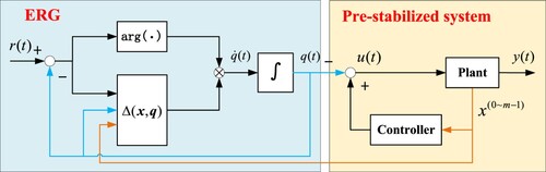The structure of control system is shown in Figure 1.

Figure 1. The structure of control system: the pre-stabilised system is represented by yellow area and the ERG is represented by blue area.

Step 1. Given that $g(x^{(0\sim m-1)},t)$ satisfies the fully actuated property (2(2) $\begin{array}{rl}& \mathrm{rank}g(x^{(0\sim m-1)},t)=n,\mathrm{\forall t}\ge 0,\mathrm{\forall }{x}^{(i)}\in {\mathbf{R}}^n,\\ & i=0,1,\dots ,m-1.\end{array}$(2) ), a generalised nonlinear PD controller for system (1(1) $\begin{array}{r}{x}^{(m)}=f(x^{(0\sim m-1)},t)+g(x^{(0\sim m-1)},t)u,\end{array}$(1) ) is designed as (5) $\begin{array}{r}\{\begin{array}{l}u=-g^{-1}(x^{(0\sim m-1)},t)[f(x^{(0\sim m-1)},t)+v],\\ v=A_0(x-r(t))+\sum _{i=1}^{m-1}{A}_i{x}^{(i)},\end{array}\end{array}$(5) where $A_0$ and $A_i,i=1,2,\dots ,m-1$ are the proportional gain and the differential gain to be designed, and $r(t)$ is a given reference signal. Under controller (5(5) $\begin{array}{r}\{\begin{array}{l}u=-g^{-1}(x^{(0\sim m-1)},t)[f(x^{(0\sim m-1)},t)+v],\\ v=A_0(x-r(t))+\sum _{i=1}^{m-1}{A}_i{x}^{(i)},\end{array}\end{array}$(5) ), the closed-loop system becomes (6) $\begin{array}{r}{x}^{(m)}=-\sum _{i=0}^{m-1}{A}_i{x}^{(i)}+A_{0}r(t).\end{array}$(6) Step 2. To prevent the violation of state constraints (3(3) $\begin{array}{r}{c}_{\mathrm{xj}}^T{x}^{(0\sim m-1)}+c_{\mathrm{ej}}^T{x}_e\le h_j,j=1,2,\dots ,n_c,\end{array}$(3) ), an ERG is designed as (7) $\begin{array}{r}\dot{q}(t)=k\mathrm{\Delta }(x,x_e)\frac{r(t)-q(t)}{max\{\Vert r(t)-q(t)\Vert ,\eta \}},\end{array}$(7) where k>0 is a constant gain and $\eta >0$ is an arbitrarily small scalar. $\mathrm{\Delta }(x,x_e)\ge 0$ is a scalar function called the dynamic safety margin, which represents the distance between the boundary of constraint set (4(4) $\begin{array}{rl}& \mathrm{\Gamma }=\{x^{(0\sim m-1)}\in {\mathbf{R}}^{\mathrm{mn}}|c_{\mathrm{xj}}^T{x}^{(0\sim m-1)}+c_{\mathrm{ej}}^T{x}_e-h_j\le 0,\\ & j=1,2,\dots ,n_c\}.\end{array}$(4) ) and the system state. $max\{\Vert r(t)-q(t)\Vert ,\eta \}$ represents that the maximum between $\Vert r(t)-q(t)\Vert$ and η is taken to prevent the denominator in Equation (7(7) $\begin{array}{r}\dot{q}(t)=k\mathrm{\Delta }(x,x_e)\frac{r(t)-q(t)}{max\{\Vert r(t)-q(t)\Vert ,\eta \}},\end{array}$(7) ) from being zero. Since the reference $r(t)$ is modified as $q(t)$, the equilibrium of the closed-loop system (6(6) $\begin{array}{r}{x}^{(m)}=-\sum _{i=0}^{m-1}{A}_i{x}^{(i)}+A_{0}r(t).\end{array}$(6) ) is transformed into $x_e=q(t)$.

To ensure that the closed-loop system (6(6) $\begin{array}{r}{x}^{(m)}=-\sum _{i=0}^{m-1}{A}_i{x}^{(i)}+A_{0}r(t).\end{array}$(6) ) is asymptotically stable, the following lemma is given to determine the gain matrices $A_i,i=0,1,\dots ,m-1$.

Lemma 2.1

Duan, 2020c

Assume that there exist $F,V\in {\mathbf{R}}^{\mathrm{mn}\times \mathrm{mn}}$ such that $\mathrm{\Phi }(A_{0\sim m-1})V=\mathrm{VF}$ and $detV\ne 0$, then (8) $\begin{array}{r}{A}_{0\sim m-1}=-Z{F}^m{V}^{-1},\end{array}$(8) where $\begin{array}{r}V=V(Z,F)=\left[\begin{array}{c}Z\\ \mathrm{ZF}\\ ⋮\\ Z{F}^{m-1}\end{array}\right],\end{array}$and $Z\in {\mathbf{R}}^{n\times \mathrm{mn}}$ is an arbitrary matrix satisfying $detV(Z,F)\ne 0$.

Remark 2.1

The ERG equation (7(7) $\begin{array}{r}\dot{q}(t)=k\mathrm{\Delta }(x,x_e)\frac{r(t)-q(t)}{max\{\Vert r(t)-q(t)\Vert ,\eta \}},\end{array}$(7) ) is composed of the constant gain k, the safety margin function $\mathrm{\Delta }(x,x_e)$ and the direction function $\frac{r(t)-q(t)}{max\{\Vert r(t)-q(t)\Vert ,\eta \}}$. Theoretically, the constant gain k should be chosen as large as possible to improve the convergence rate of $q(t)$ to $r(t)$. However, the convergence rate is also constrained by the safety margin function $\mathrm{\Delta }(x,x_e)$, which implies that the convergence rate of $q(t)$ to $r(t)$ will not improve infinitely with the increase of k. On the other hand, an excessive k will cause the ERG to be sensitive, resulting in the poor robustness of the closed-loop system. The direction function $\frac{r(t)-q(t)}{max\{\Vert r(t)-q(t)\Vert ,\eta \}}$ determines the change direction of the modified reference $q(t)$. Specifically, the reference $q(t)$ will increase if $q(t)<r(t)$, and the reference $q(t)$ will decrease if $q(t)>r(t)$. The scalar η should be chosen as small as possible to reduce its effect on the convergence performance of $q(t)$ to $r(t)$.

Remark 2.2

The main advantage of the HOFAS approach is that the full-actuation property allows us to design a controller to eliminate all the original system dynamics and construct a desired linear constant closed-loop system. However, if there exist state constraints, the designed controller cannot ensure that the system state always remains within a given constraint set. Section 6 in Duan (2022a) presents an eigenstructure-based solution to the problem, that is, the system state is restricted within a given set Ω belonging to the constraint set Γ, and the region of Ω can be maximised by optimising the parametric matrix Z. Nevertheless, the eigenstructure-based method reduces the degree of freedom of controller design, and requires the initial state of system to be within the given set Ω. In this paper, by designing an ERG, the system state can be driven to any position in the constraint set Γ, as long as the initial state belongs to Γ. Moreover, the control gain matrix $A_i$ can still be directly obtained by solving Equation (8(8) $\begin{array}{r}{A}_{0\sim m-1}=-Z{F}^m{V}^{-1},\end{array}$(8) ), and the free parametric matrix Z is no longer optimised.

3. Main results

In this section, we will give the main results of this paper. Firstly, Lemma 3.1 is provided to characterise the state constraints (3(3) $\begin{array}{r}{c}_{\mathrm{xj}}^T{x}^{(0\sim m-1)}+c_{\mathrm{ej}}^T{x}_e\le h_j,j=1,2,\dots ,n_c,\end{array}$(3) ) by the level set of the Lyapunov function, and further the dynamic safety margin function $\mathrm{\Delta }(x,x_e)$ is determined. Then we prove that, with the designed controller (5(5) $\begin{array}{r}\{\begin{array}{l}u=-g^{-1}(x^{(0\sim m-1)},t)[f(x^{(0\sim m-1)},t)+v],\\ v=A_0(x-r(t))+\sum _{i=1}^{m-1}{A}_i{x}^{(i)},\end{array}\end{array}$(5) ) and ERG (7(7) $\begin{array}{r}\dot{q}(t)=k\mathrm{\Delta }(x,x_e)\frac{r(t)-q(t)}{max\{\Vert r(t)-q(t)\Vert ,\eta \}},\end{array}$(7) ), the state of system (1(1) $\begin{array}{r}{x}^{(m)}=f(x^{(0\sim m-1)},t)+g(x^{(0\sim m-1)},t)u,\end{array}$(1) ) can asymptotically track to the reference $q(t)$ without violating the given state constraints (3(3) $\begin{array}{r}{c}_{\mathrm{xj}}^T{x}^{(0\sim m-1)}+c_{\mathrm{ej}}^T{x}_e\le h_j,j=1,2,\dots ,n_c,\end{array}$(3) ), and the modified reference $q(t)$ will converge to the original reference $r(t)$ as much as possible.

Lemma 3.1

Consider system (1(1) $\begin{array}{r}{x}^{(m)}=f(x^{(0\sim m-1)},t)+g(x^{(0\sim m-1)},t)u,\end{array}$(1) ) subject to constraints (3(3) $\begin{array}{r}{c}_{\mathrm{xj}}^T{x}^{(0\sim m-1)}+c_{\mathrm{ej}}^T{x}_e\le h_j,j=1,2,\dots ,n_c,\end{array}$(3) ). If the corresponding quadratic Lyapunov function is constructed as (9) $\begin{array}{rl}V(x^{(0\sim m-1)},x_e)& =(x-x_e{)}^{\mathrm{T}}{P}_0(x-x_e)\\ & +\sum _{i=1}^{m-1}{x^{(i)}}^{\mathrm{T}}{P}_i{x}^{(i)},\end{array}$(9) where $P_i\in {\mathbf{R}}^{n\times n}>0,i=0,\dots ,m-1$, the constraints $c_{\mathrm{xj}}^T{x}^{(0\sim m-1)}+c_{\mathrm{ej}}^T{x}_e\le h_j$ imply that the Lyapunov function is constrained to $V(x^{(0\sim m-1)},x_e)\le {\mathrm{\Gamma }}_j(x_e)$ with (10) $\begin{array}{r}{\mathrm{\Gamma }}_j(x_e)=\frac{(({\tilde{c}}_{\mathrm{xj}}^T+c_{\mathrm{ej}}^T)x_e-h_j{)}^2}{c_{\mathrm{xj}}^T{\mathrm{\Lambda }}^{-1}{c}_{\mathrm{xj}}},\end{array}$(10) where ${\tilde{c}}_{\mathrm{xj}}$ is the first n rows of $c_{\mathrm{xj}}$.

Proof.

Letting $\mathrm{\Lambda }=\mathrm{diag}\{P_i\}$, the Lyapunov function (9(9) $\begin{array}{rl}V(x^{(0\sim m-1)},x_e)& =(x-x_e{)}^{\mathrm{T}}{P}_0(x-x_e)\\ & +\sum _{i=1}^{m-1}{x^{(i)}}^{\mathrm{T}}{P}_i{x}^{(i)},\end{array}$(9) ) can be rewritten as (11) $\begin{array}{r}V(x^{(0\sim m-1)},x_e)={\left[\begin{array}{c}x-x_e\\ x^{(1\sim m-1)}\end{array}\right]}^{\mathrm{T}}\mathrm{\Lambda }\left[\begin{array}{c}x-x_e\\ x^{(1\sim m-1)}\end{array}\right].\end{array}$(11) By using a coordinate transformation $\begin{array}{r}\tilde{x}={\mathrm{\Lambda }}^{1/2}\left[\begin{array}{c}x-x_e\\ x^{(1\sim m-1)}\end{array}\right],\end{array}$we obtain that the Lyapunov function (11(11) $\begin{array}{r}V(x^{(0\sim m-1)},x_e)={\left[\begin{array}{c}x-x_e\\ x^{(1\sim m-1)}\end{array}\right]}^{\mathrm{T}}\mathrm{\Lambda }\left[\begin{array}{c}x-x_e\\ x^{(1\sim m-1)}\end{array}\right].\end{array}$(11) ) is equivalent to $V={\tilde{x}}^{\mathrm{T}}\tilde{x}$, and $x^{(0\sim m-1)}={\mathrm{\Lambda }}^{-1/2}\tilde{x}+[x_e^{\mathrm{T}}0{\cdots 0]}^{\mathrm{T}}$. Substituting the expression of $x^{(0\sim m-1)}$ into constraints $c_{\mathrm{xj}}^T{x}^{(0\sim m-1)}+c_{\mathrm{ej}}^T{x}_e-h_j\le 0$ yields that $\begin{array}{r}{c}_{\mathrm{xj}}^T{\mathrm{\Lambda }}^{-1/2}\tilde{x}+({\tilde{c}}_{\mathrm{xj}}^T+c_{\mathrm{ej}}^T)x_e-h_j\le 0.\end{array}$Thus, the boundaries of constraint set Γ are determined by the following hyperplane: $\begin{array}{r}{c}_{\mathrm{xj}}^T{\mathrm{\Lambda }}^{-1/2}\tilde{x}+({\tilde{c}}_{\mathrm{xj}}^T+c_{\mathrm{ej}}^T)x_e-h_j=0.\end{array}$Therefore, the maximum level set of Lyapunov function (9(9) $\begin{array}{rl}V(x^{(0\sim m-1)},x_e)& =(x-x_e{)}^{\mathrm{T}}{P}_0(x-x_e)\\ & +\sum _{i=1}^{m-1}{x^{(i)}}^{\mathrm{T}}{P}_i{x}^{(i)},\end{array}$(9) ) is the square distance between the origin and this hyperplane, i.e. Equation (10(10) $\begin{array}{r}{\mathrm{\Gamma }}_j(x_e)=\frac{(({\tilde{c}}_{\mathrm{xj}}^T+c_{\mathrm{ej}}^T)x_e-h_j{)}^2}{c_{\mathrm{xj}}^T{\mathrm{\Lambda }}^{-1}{c}_{\mathrm{xj}}},\end{array}$(10) ).

Based on Lemma 3.1, the state constraints (3(3) $\begin{array}{r}{c}_{\mathrm{xj}}^T{x}^{(0\sim m-1)}+c_{\mathrm{ej}}^T{x}_e\le h_j,j=1,2,\dots ,n_c,\end{array}$(3) ) can be transformed into the constraints $V(x^{(0\sim m-1)},x_e)\le {\mathrm{\Gamma }}_j(x_e)$. 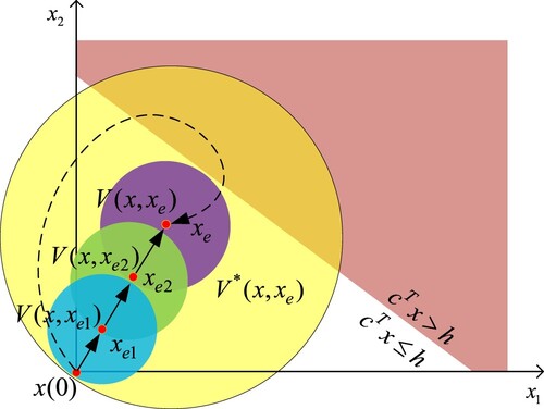Furthermore, the dynamic safety margin function is determined by (12) $\begin{array}{r}\mathrm{\Delta }(x,x_e)=min\{{\mathrm{\Gamma }}_j(x_e)-V(x^{(0\sim m-1)},x_e)\}.\end{array}$(12) We take a two-dimensional system to explain the mechanism of ERG. Assume that the initial state $x(0)$ is the origin, the final equilibrium is $x_e$, and the system state is constrained to $c^{T}x\le h$. Then there are two paths converging to $x_e$ from $x(0)$ in Figure 2. If $x(0)$ converges directly to $x_e$ (black dotted line with arrow), the state trajectory of system may exceed the constraint set, given that part of the level set of $V^{\ast }(x,x_e)$ falls outside the constraint set. An alternative approach is to change the position of equilibrium $x_e$ by modifying the reference signal such that $x(0)$ gradually converges to $x_e$ through $x_{e1}$ and $x_{e2}$ (black solid line with arrow). Since the level sets of $V(x,x_{e1})$, $V(x,x_{e2})$ and $V(x,x_e)$ are all inside the constraint set, the state trajectory of system will remain within these three level sets and never reach outside the constraint set.

Figure 2. Geometric interpretation of the ERG design scheme: $c^{T}x>h$ (red area) indicates outside the constraint set, while $c^{T}x\le h$ (white area) indicates inside the constraint set; blue area, green area, purple area and yellow area are the level sets of the Lyapunov function $V(x,x_{e1})$, $V(x,x_{e2})$, $V(x,x_e)$ and $V^{\ast }(x,x_e)$, respectively; $x(0)$ is the initial state; black solid and dotted lines with arrow represent the state trajectories of system.

Remark 3.1

The core of ERG is to characterise the constraints in the state space by the level set of the Lyapunov function. Then, the reference signal is modified to change the position of equilibrium such that the level set of the Lyapunov function is within the given constraints set at all times. Therefore, the system state can remain within the constraint set by tracking the modified reference signal.

Theorem 3.2

Consider system (1(1) $\begin{array}{r}{x}^{(m)}=f(x^{(0\sim m-1)},t)+g(x^{(0\sim m-1)},t)u,\end{array}$(1) ) subject to constraints (3(3) $\begin{array}{r}{c}_{\mathrm{xj}}^T{x}^{(0\sim m-1)}+c_{\mathrm{ej}}^T{x}_e\le h_j,j=1,2,\dots ,n_c,\end{array}$(3) ) and a given reference signal $r(t)$. The nonlinear PD controller (5(5) $\begin{array}{r}\{\begin{array}{l}u=-g^{-1}(x^{(0\sim m-1)},t)[f(x^{(0\sim m-1)},t)+v],\\ v=A_0(x-r(t))+\sum _{i=1}^{m-1}{A}_i{x}^{(i)},\end{array}\end{array}$(5) ) can ensure that the closed-loop system (6(6) $\begin{array}{r}{x}^{(m)}=-\sum _{i=0}^{m-1}{A}_i{x}^{(i)}+A_{0}r(t).\end{array}$(6) ) is asymptotically stable with the equilibrium $x_e$. Furthermore, if the reference signal $r(t)$ is modified as $q(t)$ accordingly with ERG (7(7) $\begin{array}{r}\dot{q}(t)=k\mathrm{\Delta }(x,x_e)\frac{r(t)-q(t)}{max\{\Vert r(t)-q(t)\Vert ,\eta \}},\end{array}$(7) ) and the initial reference $q(0)=x_e(0)$ satisfies $V(x(0),x_e(0))\le {\mathrm{\Gamma }}_j(x_e(0))$, the system state $x^{(0\sim m-1)}$ will not exceed the constraint set (4(4) $\begin{array}{rl}& \mathrm{\Gamma }=\{x^{(0\sim m-1)}\in {\mathbf{R}}^{\mathrm{mn}}|c_{\mathrm{xj}}^T{x}^{(0\sim m-1)}+c_{\mathrm{ej}}^T{x}_e-h_j\le 0,\\ & j=1,2,\dots ,n_c\}.\end{array}$(4) ), and $q(t)$ will converge to $r(t)$ as much as possible.

Proof.

The proof is divided into the following three parts.

Part 1: We first prove that the closed-loop system (6(6) $\begin{array}{r}{x}^{(m)}=-\sum _{i=0}^{m-1}{A}_i{x}^{(i)}+A_{0}r(t).\end{array}$(6) ) is asymptotically stable with the equilibrium $x_e$. The closed-loop system (6(6) $\begin{array}{r}{x}^{(m)}=-\sum _{i=0}^{m-1}{A}_i{x}^{(i)}+A_{0}r(t).\end{array}$(6) ) can be rewritten as (13) $\begin{array}{rl}{x}^{(1\sim m)}& =\mathrm{\Phi }(A_{0\sim m-1})x^{(0\sim m-1)}\\ & +{\left[\begin{array}{cccc}0& \cdots & 0& A_0^{\mathrm{T}}\end{array}\right]}^{\mathrm{T}}r(t).\end{array}$(13) According to the equilibrium $x_e=r(t)$, system (13(13) $\begin{array}{rl}{x}^{(1\sim m)}& =\mathrm{\Phi }(A_{0\sim m-1})x^{(0\sim m-1)}\\ & +{\left[\begin{array}{cccc}0& \cdots & 0& A_0^{\mathrm{T}}\end{array}\right]}^{\mathrm{T}}r(t).\end{array}$(13) ) is equivalent to (14) $\begin{array}{r}\left[\begin{array}{c}{x}^{(1)}\\ x^{(2)}\\ ⋮\\ x^{(m)}\end{array}\right]=\mathrm{\Phi }(A_{0\sim m-1})\left[\begin{array}{c}x\\ x^{(1)}\\ ⋮\\ x^{(m-1)}\end{array}\right]+\left[\begin{array}{c}0\\ ⋮\\ 0\\ A_0{x}_e\end{array}\right].\end{array}$(14) Further, system (14(14) $\begin{array}{r}\left[\begin{array}{c}{x}^{(1)}\\ x^{(2)}\\ ⋮\\ x^{(m)}\end{array}\right]=\mathrm{\Phi }(A_{0\sim m-1})\left[\begin{array}{c}x\\ x^{(1)}\\ ⋮\\ x^{(m-1)}\end{array}\right]+\left[\begin{array}{c}0\\ ⋮\\ 0\\ A_0{x}_e\end{array}\right].\end{array}$(14) ) can be transformed into (15) $\begin{array}{r}{x}^{(1\sim m)}=\mathrm{\Phi }(A_{0\sim m-1})\left[\begin{array}{c}x-x_e\\ x^{(1\sim m-1)}\end{array}\right].\end{array}$(15) Based on Lemma 2.1, $\mathrm{\Phi }(A_{0\sim m-1})V=\mathrm{VF}$, selecting a diagonal matrix F whose all diagonal elements are negative, the matrix $\mathrm{\Phi }(A_{0\sim m-1})$ is Hurwitz and system (15(15) $\begin{array}{r}{x}^{(1\sim m)}=\mathrm{\Phi }(A_{0\sim m-1})\left[\begin{array}{c}x-x_e\\ x^{(1\sim m-1)}\end{array}\right].\end{array}$(15) ) is asymptotically stable. Therefore, the closed-loop system (6(6) $\begin{array}{r}{x}^{(m)}=-\sum _{i=0}^{m-1}{A}_i{x}^{(i)}+A_{0}r(t).\end{array}$(6) ) is asymptotically stable with the equilibrium $x_e$.

Part 2: The system state will be proved to remain within the constraint set Γ. In view of the results in Lemma 3.1, it can be concluded that the system state will remain within the constraint set Γ if the inequality $V(x^{(0\sim m-1)},x_e)\le {\mathrm{\Gamma }}_j(x_e)$ holds. The proof will be completed by contradiction. Assume that there exist three times $t_0,t_1,t_2$ satisfying $t_0\le t_1<t_2$ such that $V(t_0)\le {\mathrm{\Gamma }}_j(t_0)$ and $V(t_2)>{\mathrm{\Gamma }}_j(t_2)$. Since $V(x^{(0\sim m-1)},x_e)$ and ${\mathrm{\Gamma }}_j(x_e)$ are continuous-time functions, it must be $V(t_1)={\mathrm{\Gamma }}_j(t_1)$. It follows from the dynamic safety margin function (12(12) $\begin{array}{r}\mathrm{\Delta }(x,x_e)=min\{{\mathrm{\Gamma }}_j(x_e)-V(x^{(0\sim m-1)},x_e)\}.\end{array}$(12) ) and ERG (7(7) $\begin{array}{r}\dot{q}(t)=k\mathrm{\Delta }(x,x_e)\frac{r(t)-q(t)}{max\{\Vert r(t)-q(t)\Vert ,\eta \}},\end{array}$(7) ) that $\mathrm{\Delta }(x(t_1),x_e(t_1))=0$ and $\dot{q}(t_1)=0$. According to the expression of ${\mathrm{\Gamma }}_j(x_e)$, we have ${\dot{\mathrm{\Gamma }}}_j(t_1)=0$. Since $\mathrm{\Phi }(A_{0\sim m-1})$ is Hurwitz, we can get $\dot{V}(x^{(0\sim m-1)},x_e)\le 0$ and $\dot{V}(t_1)\le {\dot{\mathrm{\Gamma }}}_j(t_1)$. This implies that $V(x^{(0\sim m-1)},x_e)$ will never exceed ${\mathrm{\Gamma }}_j(x_e)$, which contradicts the assumption $V(t_2)>{\mathrm{\Gamma }}_j(t_2)$. Thus, the system state will remain within the constraint set Γ.

Part 3: Finally, we prove that the modified reference $q(t)$ will converge to the original reference $r(t)$ as much as possible. The proof will be divided into the following two cases.

Case I: $\mathrm{\Delta }(x,x_e)\ge 0$. If $\mathrm{\Delta }(x,x_e)>0$, it follows from ERG (7(7) $\begin{array}{r}\dot{q}(t)=k\mathrm{\Delta }(x,x_e)\frac{r(t)-q(t)}{max\{\Vert r(t)-q(t)\Vert ,\eta \}},\end{array}$(7) ) that $\dot{q}(t)>0$ when $q(t)<r(t)$ and $\dot{q}(t)<0$ when $q(t)>r(t)$. Furthermore, if $\mathrm{\Delta }(x,x_e)=0$ and $\mathrm{\Delta }(x,x_e)\not\equiv 0$, $\mathrm{\Delta }(x,x_e)=0$ will eventually be transformed into $\mathrm{\Delta }(x,x_e)>0$ according to the results in Part 2. Therefore, $q(t)$ will converge to $r(t)$ as $x\to x_e$.

Case II: $\mathrm{\Delta }(x,x_e)\equiv 0$. It means that $q(t)\equiv r(t)$ or $V(x^{(0\sim m-1)},x_e)\equiv {\mathrm{\Gamma }}_j(x_e)$. $q(t)\equiv r(t)$ implies that the modified reference $q(t)$ has converged to $r(t)$. In what follows, the condition $V(x^{(0\sim m-1)},x_e)\equiv {\mathrm{\Gamma }}_j(x_e)$ is highlighted for discussion. In this case, the level set of the Lyapunov function is tangent to the boundaries of the constraint set Γ, that is, the modified reference $q(t)$ cannot proceed any further to $r(t)$ without violating the dynamic safety margin, given that the original equilibrium $x_e$ of the closed-loop system falls outside the constraint set Γ. Then, the reference $q(t)$ will converge to a new reference $q^{\ast }$ rather than the original reference $r(t)$, where $q^{\ast }$ is the point on the boundary of the constraint set Γ. In view of the structure of ERG (7(7) $\begin{array}{r}\dot{q}(t)=k\mathrm{\Delta }(x,x_e)\frac{r(t)-q(t)}{max\{\Vert r(t)-q(t)\Vert ,\eta \}},\end{array}$(7) ), $q(t)$ will converge towards $r(t)$ as much as possible along the direction of $r(t)-q(t)$. Since the state constraints (3(3) $\begin{array}{r}{c}_{\mathrm{xj}}^T{x}^{(0\sim m-1)}+c_{\mathrm{ej}}^T{x}_e\le h_j,j=1,2,\dots ,n_c,\end{array}$(3) ) are convex, the constraint set Γ is a convex set. Therefore, the reference $q(t)$ will approach $r(t)$ as much as possible in this convex set, and $q^{\ast }$ is the reference closest to $r(t)$.

4. Numerical examples

4.1. Example 1

In this subsection, the numerical simulation is carried out by the model in Duan (2022b) to demonstrate the effectiveness of the proposed control scheme. Consider the following nonlinear system: $\begin{array}{r}\{\begin{array}{l}{\dot{x}}_1=x_1+x_2^3,\\ {\dot{x}}_2=u.\end{array}\end{array}$Since the linearised system has an uncontrollable mode whose eigenvalue is positive, there does not exist a smooth state feedback stabilising controller in the state-space model. In Duan (2022b), the stabilisation problem of the system has been solved by the HOFAS approach. However, the tracking control problem is different from the stabilisation problem for the system. Taking first-order differential to the first equation of the system and rewriting $x_1$ as x, the system can be transformed into the following second-order fully actuated model: $\begin{array}{r}\ddot{x}=\dot{x}+3(\dot{x}-x{)}^{2/3}u.\end{array}$Given a constant reference signal $r(t)=r$, the controller is designed as $\begin{array}{r}u=-\frac{1}{3(\dot{x}-x{)}^{2/3}}(a_1\dot{x}+a_0(x-r)).\end{array}$Then the closed-loop system becomes $\begin{array}{r}\ddot{x}=-a_1\dot{x}-a_0(x-r).\end{array}$Note that the controller is effective if and only if $\dot{x}\ne x$. 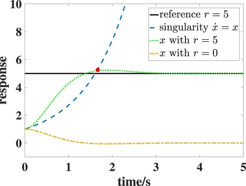For the stabilisation of the system, Duan (2022b) has proved that if the initial state satisfies $\dot{x}(0)\ne x(0)$, it can obtain $\dot{x}(t)\ne x(t)$ for any t>0, since the state trajectory of the closed-loop system and the singularity trajectory of the system $\dot{x}=x$ are opposite in direction. However, the results may no longer be reasonable in the tracking control of the system. Select $a_0=5$, $a_1=3$, $x(0)=1$, and $\dot{x}(0)=0$. Figure 3 shows the state trajectories x of the closed-loop system with r=5 and r=0, respectively. It can be seen from the figure that if the reference is r=5, there exists an intersection point (red dot) between the state trajectory x and the singularity trajectory $\dot{x}=x$ excepting for the initial point $x(0)$, since the state trajectory and the singularity trajectory are same in direction. Thus, $\dot{x}(0)\ne x(0)$ cannot guarantee $\dot{x}(t)\ne x(t)$ in the tracking control of the system. In what follows, the ERG is employed to deal with the problem.

Figure 3. The state trajectories $x(t)$ with r=5 and r=0, and the singularity trajectory $\dot{x}=x$.

Given that the initial state $\dot{x}(0)<x(0)$, to avoid the singular condition $\dot{x}(t)=x(t)$, the system state is constrained to $\dot{x}(t)<x(t),t>0$. The constraint set is determined by $\mathrm{\Gamma }=\{x|\left[\begin{array}{cc}-1& 1\end{array}\right]x^{(0\sim 1)}<0\}$, and we have $c_{\mathrm{xj}}^{\mathrm{T}}=[-11]$, ${\tilde{c}}_{\mathrm{xj}}=-1$, $c_{\mathrm{ej}}=0$ and $h_j=0$. In view of $a_0=5$, $a_1=3$, solving the Lyapunov equation $\mathrm{\Lambda \Phi }+{\mathrm{\Phi }}^T\mathrm{\Lambda }=-I$, we can obtain $\begin{array}{r}\mathrm{\Lambda }=\left[\begin{array}{cc}1.3& 0.1\\ 0.1& 0.2\end{array}\right].\end{array}$Substituting the expressions of $c_{\mathrm{xj}}$, ${\tilde{c}}_{\mathrm{ej}}$, $h_j$ and Λ into Equation (10(10) $\begin{array}{r}{\mathrm{\Gamma }}_j(x_e)=\frac{(({\tilde{c}}_{\mathrm{xj}}^T+c_{\mathrm{ej}}^T)x_e-h_j{)}^2}{c_{\mathrm{xj}}^T{\mathrm{\Lambda }}^{-1}{c}_{\mathrm{xj}}},\end{array}$(10) ) yields $\mathrm{\Gamma }=q^2/1.3$. Furthermore, according to Equation (12(12) $\begin{array}{r}\mathrm{\Delta }(x,x_e)=min\{{\mathrm{\Gamma }}_j(x_e)-V(x^{(0\sim m-1)},x_e)\}.\end{array}$(12) ), the dynamic safety margin function is determined by $\mathrm{\Delta }(x,q)=q^2/1.3-1.3(x-q{)}^2-0.2(x-q)\dot{x}-0.2{\dot{x}}^2$. The parameters of ERG (7(7) $\begin{array}{r}\dot{q}(t)=k\mathrm{\Delta }(x,x_e)\frac{r(t)-q(t)}{max\{\Vert r(t)-q(t)\Vert ,\eta \}},\end{array}$(7) ) are selected as k=10 and $\eta =0.1$. Then, the trajectories of system state and the modified reference $q(t)$ are shown in Figure 4. It can be inferred from the figure that if the system state directly tracks the reference r=5, the state will diverge because the closed-loop system is singular at the intersection between the state trajectory and the singularity trajectory. By designing an ERG, the system state can track to the reference r=5 by tracking the modified reference $q(t)$. 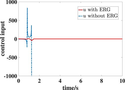Since the employment of ERG, the constraints $\dot{x}(t)<x(t)$ are satisfied and the singular condition $\dot{x}(t)=x(t)$ is avoided. Figure 5 shows the control inputs of system with ERG and without ERG, respectively. Without ERG, the control input will diverge when $\dot{x}=x$ because the controller contains the term $-1/(3(\dot{x}-x{)}^{2/3})$. Since the employment of ERG can avoid the singular condition $\dot{x}=x$, the control input with ERG is effective.

Figure 4. The state trajectories $x(t)$ with ERG and without ERG, and the references $r(t)$ and $q(t)$.

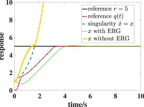
Figure 5. The control input $u(t)$ with ERG and without ERG.

4.2. Example 2

To validate further the proposed approach in this paper, consider the following nonlinear strict-feedback system in Hu and Duan (2023) with high-order form: $\begin{array}{r}\{\begin{array}{l}{x}_1^{(3)}=x_1{\dot{x}}_1^2+\cos x_1^2\sin {\ddot{x}}_1+x_2,\\ {\dot{x}}_2=\cos x_2\sin {\dot{x}}_1+{\ddot{x}}_1^2{x}_2+u,\\ y=x_1.\end{array}\end{array}$The above high-order strict-feedback system can be converted into the following form of HOFAS by elimination elevation-order $\begin{array}{r}\{\begin{array}{l}{x}_1^{(4)}=f(x_1,{\dot{x}}_1,{\ddot{x}}_1,x_1^{(3)})+u,\\ y=x_1,\end{array}\end{array}$where $f(x_1,{\dot{x}}_1,{\ddot{x}}_1,x_1^{(3)})={\dot{x}}_1^3+2x_1{\dot{x}}_1{\ddot{x}}_1-2x_1{\dot{x}}_1\sin x_1^2\sin {\ddot{x}}_1+x_1^{(3)}\cos x_1^2\cos {\ddot{x}}_1+\cos (x_1^{(3)}-x_1{\dot{x}}_1^2-\cos x_1^2\sin {\ddot{x}}_1)+{\ddot{x}}_1^2(x_1^{(3)}-x_1{\dot{x}}_1^2-\cos x_1^2\sin {\ddot{x}}_1)$. Assume that the system state is constrained to $|x_1|\le 2.1$ and the time-varying reference signal $r(t)$ is defined by $\begin{array}{r}r(t)=\{\begin{array}{l}2,0\le t<2.5,\\ 0,2.5\le t<5,\\ 2,5<t.\end{array}\end{array}$To enable the system state $x_1$ to track the given reference signal $r(t)$ and the closed-loop system to a stable linear system, the controller is designed as $\begin{array}{rl}u& =-f(x_1,{\dot{x}}_1,{\ddot{x}}_1,x_1^{(3)})-189(x_1-r(t))\\ & -130{\dot{x}}_1-60{\ddot{x}}_1-10x_1^{(3)}.\end{array}$Furthermore, to ensure that the system state satisfies the constraint $|x_1|\le 2.1$, the original reference $r(t)$ is modified as $q(t)$ by designing an ERG. According to the designed controller, the closed-loop system matrix is $\begin{array}{r}\mathrm{\Phi }=\left[\begin{array}{cccc}0& 1& 0& 0\\ 0& 0& 1& 0\\ 0& 0& 0& 1\\ -189& -130& -60& -10\end{array}\right].\end{array}$Solving the Lyapunov equation $\mathrm{\Lambda \Phi }+{\mathrm{\Phi }}^{\mathrm{T}}\mathrm{\Lambda }=-I$, we have $\begin{array}{r}\mathrm{\Lambda }=\left[\begin{array}{cccc}14.1373& 10.0790& 9.4431& 0.0030\\ 10.0790& 10.1752& 8.0520& 0.0814\\ 9.4431& 8.0520& 8.8440& 0.0570\\ 0.0030& 0.0814& 0.0570& 0.0557\end{array}\right].\end{array}$Based on Equation (12(12) $\begin{array}{r}\mathrm{\Delta }(x,x_e)=min\{{\mathrm{\Gamma }}_j(x_e)-V(x^{(0\sim m-1)},x_e)\}.\end{array}$(12) ), the dynamic safety margin function is computed by $\mathrm{\Delta }(x,q)=(q-2.1{)}^2/0.1395-14.1373(x-q{)}^2-10.1752{\dot{x}}^2-8.8440{\ddot{x}}^2-0.0557(x^{(3)}{)}^2-20.1580(x-q)\dot{x}-18.8862(x-q)\ddot{x}-0.0059(x-q)x^{(3)}-16.1040\dot{x}\ddot{x}-0.1628\dot{x}{x}^{(3)}-0.1140\ddot{x}{x}^{(3)}$. Selecting the parameters of ERG as k=0.1 and $\eta =0.01$, and the initial system state as $[x_1(0),{\dot{x}}_1(0),{\ddot{x}}_1(0),x_1^{(3)}(0)]=[0,0.3,0.5,0.3]$, the state trajectories $x_1$ of control system with ERG and without ERG are shown in Figure 6. It can be seen from the figure that, by employing the ERG technique, the state $x_1$ will track to the reference $r(t)$ and not exceed the state constraint $|x_1|\le 2.1$. By contrast, the system state $x_1$ violates the constraint $|x_1|\le 2.1$ when the control system is without ERG. The reason for this result is that we design an ERG such that the state $x_1$ tracks the modified reference $q(t)$ instead of the reference $r(t)$, which guarantees that the level set of the Lyapunov function is within the constraint set determined by $|x_1|\le 2.1$. 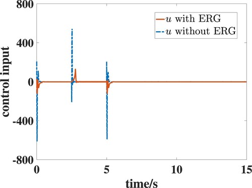Furthermore, the modified reference $q(t)$ converges to the original reference $r(t)$, which is shown in Figure 7. The control inputs of system with ERG and without ERG are shown in Figure 8, respectively. It is clear that the controller with ERG requires lower control input compared with that without ERG.

Figure 6. The state trajectory $x_1(t)$ with ERG and without ERG, and the references $r(t)$.

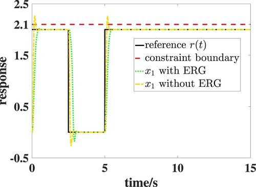
Figure 7. The original reference $r(t)$ and the modified reference $q(t)$.

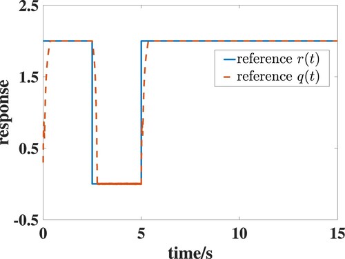
Figure 8. The control input $u(t)$ with ERG and without ERG.

5. Conclusion

In this work, we address the tracking control problem of nonlinear HOFAS with state constraints. To stabilise the system, a generalised nonlinear PD controller is designed. Then, an ERG is constructed to modify the reference signal such that the modified reference can be reached without violating the state constraints. Furthermore, we prove that the modified reference will converge to the original reference as much as possible. Finally, two numerical simulations are provided to demonstrate the validity of the proposed control scheme. This paper has deigned the control scheme for the nominal HOFAS with state constraints, but there are always some perturbations in the practical systems such as model uncertainties and external disturbances. In the future works, we will design an ERG involving perturbation information to address the robust tracking control problem of nonlinear HOFAS with state constraints and model uncertainties.

Disclosure statement

No potential conflict of interest was reported by the author(s).

Data availability statement

Data sharing not applicable to this article as no datasets were generated or analysed during the current study.

Additional information

Funding

This work is supported by National Natural Science Foundation (NNS- F) of China [Grant Nos. 62022055 and 61973215]

References

- Bemporad, A. (1998). Reference governor for constrained nonlinear systems. IEEE Transactions on Automatic Control, 43(3), 415–419. https://doi.org/10.1109/9.661611
- Duan, G. (2020a). High-order fully actuated system approaches: Part III. Observability and observer design. Acta Automatica, 46(9), 1885–1895. https://doi.org/10.16383/j.aas.c200370
- Duan, G. (2020b). High-order fully actuated system approaches: Part III. Robust control and high-order backstepping. International Journal of Systems Science, 52(5), 952–971. https://doi.org/10.1080/00207721.2020.1849863
- Duan, G. (2020c). High-order fully actuated system approaches: Part I. Models and basic procedure. International Journal of Systems Science, 52(2), 422–435. https://doi.org/10.1080/00207721.2020.1829167
- Duan, G. (2020d). High-order fully actuated system approaches: Part IV. Adaptive control and high-order backstepping. International Journal of Systems Science, 52(5), 972–989. https://doi.org/10.1080/00207721.2020.1849864
- Duan, G. (2021). High-order fully actuated system approaches: Part VII. Controllability, stabilisability and parametric designs. International Journal of Systems Science, 52(14), 3091–3114. https://doi.org/10.1080/00207721.2021.1921307
- Duan, G. (2022a). High-order fully-actuated system approaches: Part IX. Generalised PID control and model reference tracking. International Journal of Systems Science, 53(3), 652–674. https://doi.org/10.1080/00207721.2021.1970277
- Duan, G. (2022b). Stabilization via fully actuated system approach: A case study. Journal of Systems Science and Complexity, 35(3), 731–747. https://doi.org/10.1007/s11424-022-2091-7
- Garone, E., & Nicotra, M. M. (2015). Explicit reference governor for constrained nonlinear systems. IEEE Transactions on Automatic Control, 61(5), 1379–1384. https://doi.org/10.1109/TAC.2015.2476195
- Gilbert, E. G., & Kolmanovsky, I. V. (1999). Set-point control of nonlinear systems with state and control constraints: A Lyapunov-function, Reference-Governor approach. In Proceedings of the 38th IEEE conference on decision and control (pp. 2507–2512). IEEE.
- Hosseinzadeh, M., & Garone, E. (2019). An explicit reference governor for the intersection of concave constraints. IEEE Transactions on Automatic Control, 65(1), 1–11. https://doi.org/10.1109/TAC.9
- Hosseinzadeh, M., Sinopoli, B., & Bobick, A. F. (2020). An explicit reference governor for time-varying linear constraints. In Proceedings of the 59th IEEE conference on decision and control (pp. 3323–3328). IEEE.
- Hu, L., & Duan, G. (2023). Adaptive guaranteed cost tracking control for high-order nonlinear systems based on fully actuated system approaches. Transactions of the Institute of Measurement and Control. Article 01423312231183610
- Liu, X., Chen, M., Sheng, L., & Zhou, D. (2022). Adaptive fault-tolerant control for nonlinear high-order fully-actuated systems. Neurocomputing, 495, 75–85. https://doi.org/10.1016/j.neucom.2022.04.129
- Liu, Y., & Tong, S. (2017). Barrier Lyapunov functions for Nussbaum gain adaptive control of full state constrained nonlinear systems. Automatica, 76, 143–152. https://doi.org/10.1016/j.automatica.2016.10.011
- Mayne, D. Q. (2014). Model predictive control: Recent developments and future promise. Automatica, 50(12), 2967–2986. https://doi.org/10.1016/j.automatica.2014.10.128
- Meng, R., Hua, C., Li, K., & Ning, P. (2022). Adaptive event-triggered control for uncertain high-order fully actuated system. IEEE Transactions on Circuits and Systems II: Express Briefs, 69(11), 4438–4442. https://doi.org/10.1109/TCSII.2022.3177309
- Nicotra, M. M., Liao-McPherson, D., Burlion, L., & Kolmanovsky, I. V. (2019). Spacecraft attitude control with nonconvex constraints: An explicit reference governor approach. IEEE Transactions on Automatic Control, 65(8), 3677–3684. https://doi.org/10.1109/TAC.9
- Niu, B., & Zhao, J. (2013). Tracking control for output-constrained nonlinear switched systems with a barrier Lyapunov function. International Journal of Systems Science, 44(5), 978–985. https://doi.org/10.1080/00207721.2011.652222
- Tee, K. P., Ge, S. S., & Tay, E. H. (2009). Barrier Lyapunov functions for the control of output-constrained nonlinear systems. Automatica, 45(4), 918–927. https://doi.org/10.1016/j.automatica.2008.11.017
- Wang, P., Zhang, W., Zhang, X., & Ge, S. S. (2022). Robust invariance-based explicit reference control for constrained linear systems. Automatica, 143, Article 110433. https://doi.org/10.1016/j.automatica.2022.110433
- Xi, Y. (1993). Model predictive control. National Defense Industry Press.
- Yu, Y., Liu, G., Huang, Y., & Guerrero, J. M. (2023). Coordinated predictive secondary control for dc microgrids based on high-order fully actuated system approaches. IEEE Transactions on Smart Grid, 15(1), 19–33. https://doi.org/10.1109/TSG.2023.3266733
- Zhang, D., Liu, G., & Cao, L. (2022). Proportional integral predictive control of high-order fully actuated networked multiagent systems with communication delays. IEEE Transactions on Systems, Man, and Cybernetics: Systems, 53(2), 801–812. https://doi.org/10.1109/TSMC.2022.3188504
- Zhang, L., Zhu, L., & Hua, C. (2022). Practical prescribed time control based on high-order fully actuated system approach for strong interconnected nonlinear systems. Nonlinear Dynamics, 110(4), 3535–3545. https://doi.org/10.1007/s11071-022-07820-w