Improvement of a Simple Coupled VOF with LS (S-CLSVOF) Method

Abstract

In this study, an efficient conversion algorithm of level set function $\varphi$ from volume fraction $\alpha$ is developed. This method makes the calculation of $\varphi$ easier than the conventional CLSVOF method, and the precision of surface tension can be improved by the application of $\varphi .$ The two numerical tests are shown to demonstrate the proposed scheme. As a result of two demonstration tests, it is obtained that (a) the proposed method gives better $\varphi$ than that of the existing simple coupled method because this can take into account multi-dimensional profiles of $\alpha ,$ (b) a surface tension evaluated by using the proposed method can contribute to much lower spurious currents, (c) the proposed method can simulate bubble generation with a similar precision of rigorous CLSVOF method.

KEYWORD:

• Computational fluid dynamics
• Volume of fluid method
• Level set function

1. Introduction

Recently, chemical processes including a gas-liquid interface have increased in importance in the fields of printed electronics and biotechnologies, etc. The theoretical research of these processes is complicated due to the dynamical interactions between surface tension force and fluid field. To clarify the mechanism of the interactions, many numerical studies have been developed. Especially, numerical methods in the full Eulerian framework are useful because the efficient computation of fluid dynamics with complicated interface morphology can be carried out. Numerical methods for the full Eulerian framework have been developed such as Volume of Fluid (VOF), Level Set (LS), and many improved methods (Prosperetti and Tryggvason 2009). The former captures the interface by defining a volume fraction $\alpha$ in a range of $\left[0,1\right]$ where an interface is indicated in the cell with $\alpha \in \left(0,1\right).$ The latter uses the signed distance function $\varphi ,$ an interface locates at iso-surfaces or lines of $\varphi =0.$ The VOF-type method has an advantage in the conservation of volume, whereas an ingenious advection scheme must be used to avoid non-physical diffusion. Many advection schemes have been developed such as CICSAM (Compressive Interface Capturing Scheme for Arbitrary Meshes, Ubbink and Issa (1999), HRIC (High-Resolution Interface Capturing scheme, Muzaferija et al. (1998), SLIC (Simple Linear Interface Calculation, Noh and Woodward (1976)), and PLIC (Piecewise Linear Interface Calculation, Youngs 1982). The authors also developed THAINC (Tangent Hyperbola with Adaptive slope for Interface Capturing) scheme which extends a tangent hyperbola function to three-dimensional spaces (Dhar et al. 2013).

On the other hand, it is pointed out that the LS-type method cannot keep the nature of distance function $\varphi$ in the computational process of advection terms. The $\varphi$ then must be recovered by using a re-initialization procedure. In the earlier study, the re-initialization procedure might be a cause of poor conservation of volume of a focusing fluid, but Olsson et al. (2007) and Losasso et al. (2006) overcame the disadvantage by modifying the re-initialization procedure.

As for a surface tension force, Continuum Surface Force (CSF) model (Blackbill et. al.(1992)) has been used in many numerical studies. However, it is pointed out that the CSF model in the VOF method yields numerical errors (Hayashi 2007; Lafaurie et al. 1994; Renardy and Renardy 2002), whereas the use of the CSF model in the LS method decreases the error dramatically. A coupled LS and VOF (CLSVOF) method that combines the VOF method and the LS method can be a way to resolve to fix that problem. In addition, when using the CLSVOF method, we can become available both the advantage of conservation of volume and precision of surface tension force. Although the CLSVOF method is more accurate than both the standalone LS and VOF methods, an original CLSVOF method demands a larger computational cost because the calculational procedures for advection of both $\varphi$ and $\alpha ,$ and the combination of these variables are required. To simplify the coupling procedure, Kunkelmann and Stephan (2010) proposed the algorithm in which $\alpha$ is only advected and $\varphi$ is converted from the profiles of $\alpha .$ Albadawi et al. (2013) proposed a more simplified method called S-CLSVOF (A simple coupled VOF with LS method). This method allows us easy modification of existing VOF source code, and an increase of computational load is smaller than that for the original CLSVOF method. For example, Yamamoto et al. (2017) implemented the S-CLSVOF method in an open computational fluid dynamics code (OpenFOAM), and confirmed the acceptable precision of thermo-capillary flows. However, the S-CLSVOF method handles $\varphi$ and $\alpha$ without any spatial directions. In other words, the converted value of $\varphi$ can be ambiguous in multidimensional geometry problems.

In this study, we propose a novel numerical algorithm that converts the information of $\alpha$ to the information of $\varphi .$ This method makes the calculation of $\varphi$ easier than the conventional CLSVOF method, and the precision of surface tension can be improved by the application of $\varphi .$ The validation of our new numerical algorithm is shown through the following numerical tests:

1. The motion of a single bubble and drop under the condition of no-gravity

2. Bubble formation from a single nozzle

2. Numerical method

2.1. Governing equations

On the one-fluid approximation, mass and momentum conservations of two-phase incompressible fluid are given as: (1) $$\nabla \cdot \mathit{V}=0$$(1) (2) $$\rho \left(\frac{\partial \mathit{V}}{\partial t}+(\mathit{V}\cdot \nabla )\mathit{V}\right)=-\nabla P+\nabla \cdot \mu [\nabla \mathit{V}+{(\nabla \mathit{V})}^{\mathrm{T}}]+\rho \mathit{g}+{\mathit{F}}_{\sigma }$$(2) where $\mathit{V}$ is the velocity, $\rho$ the density, $t$ the time, $P$ the pressure, $\mu$ the viscosity, $\mathit{g}$ the gravity, and ${\mathit{F}}_{\sigma }$ the surface tension force at the interface. $\rho$ and $\mu$ are given by: (3) $$\rho ={\alpha }_L{\rho }_L+{\alpha }_G{\rho }_G$$(3) (4) $$\mu ={\alpha }_L{\mu }_L+{\alpha }_G{\mu }_G$$(4) where $\alpha$ is the volume fraction of phases, and subscripts $L$ and $G$ are liquid and gas, respectively.

The volume fraction $\alpha$ is transported by the following equation. (5) $$\frac{\partial \alpha }{\partial t}+\mathit{V}\cdot \nabla \alpha =0$$(5)

To solve Eq. (5)(5) $$\frac{\partial \alpha }{\partial t}+\mathit{V}\cdot \nabla \alpha =0$$(5) , we use the THAINC method. This method extends a tangent hyperbola function proposed by Xiao et al. (2005) to multi-dimension. In the Cartesian coordinate system, an interpolation of $\alpha$ in the $x$ direction can be written as: (6) $$\alpha \left(x\right)=\frac{1}{2}\left\{1+\gamma \tanh \hspace{0.17em}\beta \left(\frac{x-x_{\mathrm{edge}}}{\Delta x}-{\tilde{x}}_D\right)\right\}$$(6) where $x_{\mathrm{edge}}$ is the location at the computational cell face, $\Delta x$ the cell size. Parameters $\gamma ,$ $\beta ,$ ${\tilde{x}}_D$ can be given by (7) $$\gamma =\{\begin{array}{c}1\mathrm{ }if\mathrm{ }\partial \alpha /\partial x\ge 0\\ -1\mathrm{ }\mathit{otherwise}\end{array}$$(7) (8) $$\beta =\min \hspace{0.17em}\left[{\beta }_{\max },\max \hspace{0.17em}\left\{{\beta }_{\min },\frac{2\left|n_x\right|}{\sqrt{n_y^2}}\right\}\right]$$(8) (9) $${\tilde{x}}_D=\frac{1}{2\beta }\ln \hspace{0.17em}\left[\frac{\exp \hspace{0.17em}\left(2\beta \right)-\lambda \exp \hspace{0.17em}\left(2\beta \right)}{\lambda \exp \hspace{0.17em}\left(2\beta \right)-1}\right]$$(9) (10) $$\lambda =\exp \hspace{0.17em}\left[\frac{\beta \left(2\alpha -1\right)}{\gamma }\right]$$(10) where $n_x$ and $n_y$ are $x$ and $y$ components of interface normal, respectively. After performing some numerical experiments with different values of ${\beta }_{\min }$ and ${\beta }_{\max },$ we have found that ${\beta }_{\min }=0.001$ and ${\beta }_{\max }=10$ were reasonable values to transport $\alpha$ (Dhar et al. 2014).

2.2. Coupling of Level Set Function

Albadawi et al. (2013) proposed a calculation method that evaluates the initial value of the level set function ${\varphi }_0$ by using the following simple equation. (11) $${\varphi }_0=\left(2\alpha -1\right)\Gamma$$(11) where the parameter $\mathit{\Gamma }$ depends on the cell size. In the literature (Albadawi et al. 2013), $\mathrm{\Gamma }=0.75\Delta x$ is proposed. The profiles of $\varphi$ are calculated by using the following equation. (12) $$\frac{\partial \varphi }{\partial \tau }=\mathrm{Sign}\left({\varphi }_0\right)\left(1-\left|\nabla \varphi \right|\right)$$(12) where $\tau$ is the pseudo-time step. For example, $\tau =\Delta x/N,$ $N>10$ are recommended (Albadawi et al. 2013). Using Eq. (11)(11) $${\varphi }_0=\left(2\alpha -1\right)\Gamma$$(11) , the value of $\varphi$ converted from the information α is ambiguous in the multidimensional geometry problems. Therefore, we need to consider other alternatives to Eq. (11)(11) $${\varphi }_0=\left(2\alpha -1\right)\Gamma$$(11) : the interpolation technique in the THAINC method is utilized as an alternative method.

We shall explain the details for the one-dimensional case and multi-dimensional algorithm following analogously.

When the points of origin in Eq. (6)(6) $$\alpha \left(x\right)=\frac{1}{2}\left\{1+\gamma \tanh \hspace{0.17em}\beta \left(\frac{x-x_{\mathrm{edge}}}{\Delta x}-{\tilde{x}}_D\right)\right\}$$(6) are shifted and ${\tilde{x}}_D$ is displaced with ${\varphi }_i\mathrm{ }\left(i=x,y\mathrm{ }or\mathrm{ }z\right),$ we obtain: (13) $$\alpha \left(x\right)=\frac{1}{2}\left\{1+\gamma \tanh \hspace{0.17em}\beta \left(\frac{x}{\Delta x}-{\varphi }_x\right)\right\}$$(13) for the $x$ direction. By integrating $\alpha \left(x\right)$ with $x,$ we give the following condition. (14) $$\frac{1}{\mathrm{\Delta }x}{\int }_{-0.5\mathrm{\Delta }x}^{0.5\mathrm{\Delta }x}\alpha \left(x\right)dx={\alpha }_{\mathrm{VOF}}$$(14) where ${\alpha }_{\mathrm{VOF}}$ is the calculated value by the VOF method. By substituting Eq. (13)(13) $$\alpha \left(x\right)=\frac{1}{2}\left\{1+\gamma \tanh \hspace{0.17em}\beta \left(\frac{x}{\Delta x}-{\varphi }_x\right)\right\}$$(13) in Eq. (14)(14) $$\frac{1}{\mathrm{\Delta }x}{\int }_{-0.5\mathrm{\Delta }x}^{0.5\mathrm{\Delta }x}\alpha \left(x\right)dx={\alpha }_{\mathrm{VOF}}$$(14) , we obtain: (15) $${\varphi }_x=\frac{1}{2\beta }\ln \hspace{0.17em}\left[\frac{e^{\beta }-\lambda }{\lambda e^{\beta }-1}\right]$$(15) (16) $$\lambda =\exp \hspace{0.17em}\left[\frac{\beta \left(2{\alpha }_{\mathrm{VOF}}-1\right)}{\gamma }\right]$$(16)

In Eq. (15)(15) $${\varphi }_x=\frac{1}{2\beta }\ln \hspace{0.17em}\left[\frac{e^{\beta }-\lambda }{\lambda e^{\beta }-1}\right]$$(15) , $\beta$ can be estimated by Eq. (8)(8) $$\beta =\min \hspace{0.17em}\left[{\beta }_{\max },\max \hspace{0.17em}\left\{{\beta }_{\min },\frac{2\left|n_x\right|}{\sqrt{n_y^2}}\right\}\right]$$(8) . Here, a demonstration of the conversion of $\varphi$ from the various $\alpha$ is performed in the one-dimensional case where $\alpha$ is located perpendicular to the x-axis. Hereafter, the unit grid size is used ($\mathrm{\Delta }x=1$). 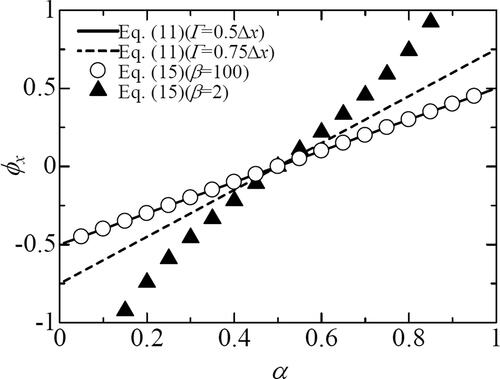The results are shown in Figure 1, where the solid line is ϕ obtained by Eq. (11)(11) $${\varphi }_0=\left(2\alpha -1\right)\Gamma$$(11) with Γ = 0.50Δx and the dashed line is ϕ obtained using that with Γ = 0.75Δx. Open circle and solid triangle correspond to results obtained using Eq. (15)(15) $${\varphi }_x=\frac{1}{2\beta }\ln \hspace{0.17em}\left[\frac{e^{\beta }-\lambda }{\lambda e^{\beta }-1}\right]$$(15) . From Figure 1, it is obvious that $\varphi$ obtained by Eq. (15)(15) $${\varphi }_x=\frac{1}{2\beta }\ln \hspace{0.17em}\left[\frac{e^{\beta }-\lambda }{\lambda e^{\beta }-1}\right]$$(15) changes from –0.5 to 0.5 linearly when ${\beta }_{\max }=100$ is set. The result agrees well with the correct ${\varphi }_x.$ Namely, ${\beta }_{\max }=100$ is selected in this study.

Figure 1. Variation of ${\varphi }_x$ as a function of α .

Next, the extension to the two-dimensional case will be discussed. Since $\alpha$ is a scalar variable, Eq. (11)(11) $${\varphi }_0=\left(2\alpha -1\right)\Gamma$$(11) cannot reflect the distance in two dimensions. In this study, the distance in each direction (such as ${\varphi }_x$ and ${\varphi }_y$) is calculated by using Eq. (15)(15) $${\varphi }_x=\frac{1}{2\beta }\ln \hspace{0.17em}\left[\frac{e^{\beta }-\lambda }{\lambda e^{\beta }-1}\right]$$(15) . It should be noted that ${\varphi }_x$ and ${\varphi }_y$ have different values because $\beta$ varies due to the slope of the interface (i.e. Eq. (8)(8) $$\beta =\min \hspace{0.17em}\left[{\beta }_{\max },\max \hspace{0.17em}\left\{{\beta }_{\min },\frac{2\left|n_x\right|}{\sqrt{n_y^2}}\right\}\right]$$(8) ). 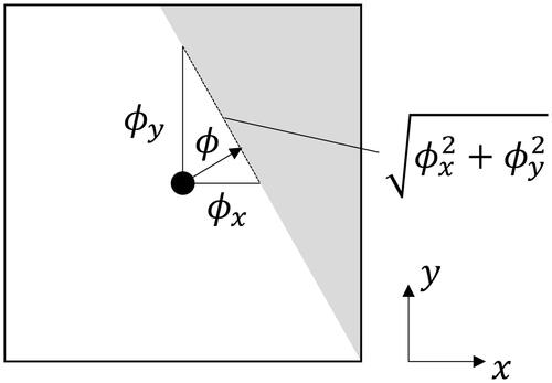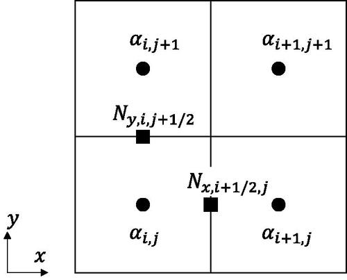This can affect the construction of $\varphi$ in the multi-dimensional problem. The value of geometrical distance $\varphi$ is then calculated by the following equation (see Figure 2): (17) $$\varphi =\frac{{\varphi }_x{\varphi }_y}{\sqrt{{\varphi }_x^2+{\varphi }_y^2}}$$(17)

Figure 2. Location of ${\varphi }_x,$ ${\varphi }_y$ and $\varphi .$

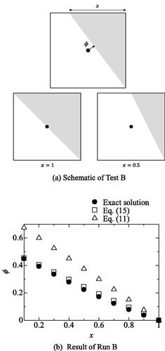
To validate the proposed method, two numerical tests are carried out. In Test A shown in Figure 3, $\alpha$ with $\alpha =0.25$ is indicated as a gray region and another is the white region. The white region is $\varphi >0,$ whereas $\varphi <0$ in the gray region. An angle of inclination is changed and the effect of $\varphi$ ware compared. The results are shown in Figure 4(a) and (b). It is clearly shown that Eq. (11)(11) $${\varphi }_0=\left(2\alpha -1\right)\Gamma$$(11) cannot essentially acquire exact $\varphi$ whereas the proposed method gives good agreement with the exact solutions. In addition, the effect of variable $\alpha$ is compared in Figure 5. The proposed method gives better $\varphi$ values than any $\alpha .$

Figure 3. Schematic of Test A.

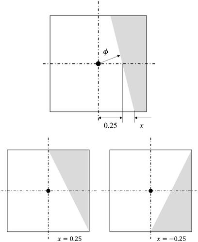
Figure 4. Two-dimensional test for $\varphi$ (Run A). (a) Result of run A. (b) Zoom of Figure 4 (a).

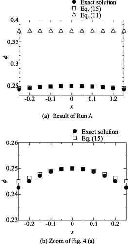
Figure 5. Two-dimensional test for $\varphi$ (Run B). (a) Schematic of test B. (b) Result of run B.

This method makes the calculation of $\varphi$ easier than the conventional CLSVOF method, and the precision of surface tension can be improved by the application of $\varphi .$

2.3. Surface tension model

From the concept of the CSF model, ${\mathit{F}}_{\sigma }$ is calculated by using: (18) $${\mathit{F}}_{\sigma }=\sigma \kappa \mathit{n}\delta$$(18) where $\sigma$ is the surface tension, $\kappa$ the curvature, $\mathit{n}$ the unit normal to the interface, and $\delta$ the delta function. Equation (18)(18) $${\mathit{F}}_{\sigma }=\sigma \kappa \mathit{n}\delta$$(18) can be rewritten as (19) $${\mathit{F}}_{\sigma }=\sigma \kappa \mathit{N}$$(19) (20) $$\mathit{N}=\nabla \alpha$$(20)

The Arrangement of $\alpha$ and $\mathit{N}$ is shown in Figure 6 Francois et al. (2006) proposed the calculation method of $\mathit{N}$ by using the following equations. (21) $$N_{x,i+1/2,j}=\frac{{\alpha }_{i+1,j}-{\alpha }_{i,j}}{\mathrm{\Delta }x}$$(21) (22) $$N_{y,i,j+1/2}=\frac{{\alpha }_{i,j+1}-{\alpha }_{i,j}}{\mathrm{\Delta }y}$$(22)

Figure 6. Variable arrangement in a cell.

In addition, $\kappa$ is interpolated by (23) $${\kappa }_{i+1/2,j}=\frac{{\kappa }_{i,j}\left|{\varphi }_{i+1,j}\right|+{\kappa }_{i+1,j}\left|{\varphi }_{i,j}\right|}{\left|{\varphi }_{i+1,j}\right|+\left|{\varphi }_{i,j}\right|}$$(23)

On the other hand, Renardy and Renardy (2002) proposed another interpolation defined by: (24) $${\kappa }_{i+1/2,j}=\frac{w_{i,j}{\kappa }_{i,j}+w_{i+1,j}{\kappa }_{i+1,j}}{w_{i,j}+w_{i+1,j}}$$(24) (25) $$w_{i,j}={\alpha }_{i,j}\left(1-{\alpha }_{i,j}\right)$$(25) $\kappa$ is estimated by: (26) $$\kappa =-\nabla \cdot \mathit{n}$$(26)

In the framework of the CSF model, the following two types of equations can be considered. (27) $${\mathit{n}}_{\alpha }=\frac{\nabla \alpha }{\left|\nabla \alpha \right|}$$(27) (28) $${\mathit{n}}_{\varphi }=\frac{\nabla \varphi }{\left|\nabla \varphi \right|}$$(28)

The detail of Eqs. (26–28) are shown in Appendix (ALE-like scheme in the Blackbill et. al. (1992). In this study, ${\mathit{F}}_{\sigma }$ is calculated with ${\mathit{n}}_{\varphi }.$ In the case where the interface contacts with walls, an extrapolation of $\varphi$ or $\alpha$ can express a contact angle. But the direct assignment of $\mathit{n}$ is a more concise procedure. (29) $$\mathit{n}={\mathit{n}}_w\cos \hspace{0.17em}\theta +{\mathit{n}}_{t\varphi }\sin \hspace{0.17em}\theta$$(29) where ${\mathit{n}}_w$ is the normal vector of walls, $\theta$ the contact angle, and ${\mathit{n}}_{t\varphi }$ the tangential vector of the contact interface.

Figure 7 shows the calculation procedure. Parts enclosed in red rectangles correspond to additional procedures to the existing VOF method. This means the modification of source code is as easy as the S-CLSVOF method. Table 1 lists the numerical schemes employed in this study. To solve Eq. (12)(12) $$\frac{\partial \varphi }{\partial \tau }=\mathrm{Sign}\left({\varphi }_0\right)\left(1-\left|\nabla \varphi \right|\right)$$(12) , the 3rd-order TVD Runge-Kutta scheme and ENO (Essentially Non-Oscillatory polynomial interpolation) scheme are adopted.

Figure 7. Calculation procedure.

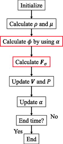
Table 1. Numerical schemes in the present study.

Term of calculation	Scheme
Advection of $\mathit{V}$	3rd order CIP scheme (Constrained Interpolation Profile Scheme)
Viscosity	Central difference
Time difference	2nd order Adams-Bashforth
Advection of $\alpha$	THAINC
Poisson equation of $P$	BiCGStab (Biconjugate Gradient Stabilized method)

3. Demonstration

3.1. The motion of a single bubble and drop under the condition of no-gravity

To demonstrate the effectiveness of the THAINC-LS method, the two-dimensional motion of a single bubble under the condition of no gravity was calculated. In addition, a droplet also was examined in the same condition.

This test was also performed by Albadawi et al. (2013) and Yamamoto et al. (2017). The calculation domain is a square of 0.05 m on a side. Surrounding all walls are defined as slip walls. A circle of 0.01 m in diameter was located at the center of the region. The numerical method in this test is shown in Table 2. The physical properties of a bubble or droplet are summarized in Table 3. Two types of computational grid size are set in this test shown in Table 4. Correct solutions consist of a zero velocity field because the pressure field is balanced at a circle due to surface tension force. Then, the following value of two errors was compared as performance indexes.

Table 2. Method for calculation of surface tension.

Method	Equations
A (CSF with VOF function)	Eq. (25)
B (Albadawi et al. 2013)	Eq. (26) with (11)
C (Proposed)	Eq. (26) with (17)

Table 3. Physical properties.

Unit	Bubble	Drop
${\rho }_1$[kg/m^3]	$1$	$1000$
${\rho }_2$[kg/m^3]	$1000$	$1$
${\mu }_1$[Pa･s]	$1\times {10}^{-5}$	$1\times {10}^{-3}$
${\mu }_2$[Pa･s]	$1\times {10}^{-3}$	$1\times {10}^{-5}$
$\mathrm{\sigma }$[N/m]	$1.0\times {10}^{-2}$	$1.0\times {10}^{-2}$

Table 4. Grid size resolution.

Level	Number of cells	$\mathrm{\Delta }x,\mathrm{\Delta }y$ [m]
L1	$50\times 50$	$0.001$
L2	$100\times 100$	$0.0005$
L3	$150\times 150$	$0.001/3$
L4	$200\times 200$	$0.00025$

(1) Maximum error of fluid velocity (30) $$\left|V_{\max }\right|=\underset{i,j}{\max }\left|{\mathit{V}}_{i,j}\right|$$(30)

(2) Cell averaged error of fluid velocity (31) $$\left|V_{\mathrm{ave}}\right|=\frac{1}{N_x{N}_y}\sum _{i,j}\left|{\mathit{V}}_{i,j}\right|$$(31) where $N_x$ and $N_y$ are the numbers of computational cells. We compared the average pressure inside the circle with Yong–Laplace’s theory. As a result, errors of pressure induced by surface tension were within 1%.

Table 5 summarizes the comparison of the value of two errors for the case of bubble and droplet at t = 0.1 s, respectively. It was confirmed that the motion of a single bubble and droplet under the condition of no-gravity was in a pseudo-steady state at t = 0.1 s. Albadawi et al. (2013) insisted that the S-CLSVOF was effective in decreasing errors, and our test results (Method B) also follow their findings. Furthermore, it is notable that the errors when using the proposed method (Method C) are the smallest compared to those for other methods. Figure 8 shows the comparison of velocity fields at t = 0.1 s. If the flow is in a completely steady state, the velocity in both phases doesn’t arise due to the balance of pressure and surface tension force. As is obvious from Figure 8, Method A gives birth to large-scale velocities. Unrealistic velocities are called spurious currents and have been identified by many researchers (e.g. Hayashi 2007 and Yokoi 2007).

Figure 8. Velocity profiles at t = 0.1 s (Bubble case, resolution:L2). (a) Numerical results obtained by the original Method A. (b) Numerical results obtained by Method B. (c) Numerical results obtained by the Method C.

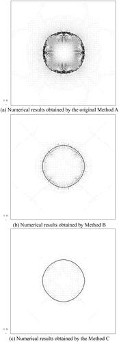
Table 5. Comparison of the value of two errors.

(a) Bubble case
Method	Resolution	$\left|V_{\max }\right|$	$\left|V_{\mathrm{ave}}\right|$
A	L1	$5.41\times {10}^{-2}$	$2.93\times {10}^{-3}$
	L2	$6.97\times {10}^{-2}$	$2.62\times {10}^{-3}$
	L3	$9.78\times {10}^{-2}$	$2.45\times {10}^{-3}$
	L4	$1.32\times {10}^{-1}$	$3.29\times {10}^{-3}$
B	L1	$1.26\times {10}^{-2}$	$4.75\times {10}^{-4}$
	L2	$2.75\times {10}^{-2}$	$5.34\times {10}^{-4}$
	L3	$3.51\times {10}^{-2}$	$5.45\times {10}^{-4}$
	L4	$3.61\times {10}^{-2}$	$3.57\times {10}^{-4}$
C	L1	$8.82\times {10}^{-3}$	$3.83\times {10}^{-4}$
	L2	$6.62\times {10}^{-3}$	$1.37\times {10}^{-4}$
	L3	$9.30\times {10}^{-3}$	$1.42\times {10}^{-4}$
	L4	$9.19\times {10}^{-3}$	$1.05\times {10}^{-4}$
(b) Drop case
Method		$\left|V_{\max }\right|$	$\left|V_{\mathrm{ave}}\right|$
A	L2	$7.35\times {10}^{-2}$	$3.37\times {10}^{-3}$
	L3	$9.63\times {10}^{-2}$	$4.27\times {10}^{-3}$
B	L2	$2.83\times {10}^{-2}$	$6.23\times {10}^{-4}$
	L3	$7.05\times {10}^{-2}$	$9.66\times {10}^{-4}$
C	L2	$4.54\times {10}^{-3}$	$1.50\times {10}^{-4}$
	L3	$4.67\times {10}^{-3}$	$1.61\times {10}^{-4}$

As can be seen from Table 4 and Figure 8, Method B can reduce spurious currents. This means that making use of $\varphi$ is effective for estimating the surface tension force. Moreover, the proposed method (Method C) can drastically reduce spurious currents with more accurate $\varphi$ values.

3.2. Bubble formation from a single nozzle

To demonstrate a more practical case, bubble formation from a single nozzle is calculated. Previously, Ohta et al. (2007, 2011) calculated this by using the original CLSVOF method. They compared with the experimental results by Helsby and Tuson (1955) and successfully obtained a good agreement on bubbles behavior. In this study, we tried to compare the calculation with that of Ohta et al. (2007, 2011).

Table 6 and Figure 9 show computational conditions and boundary conditions, respectively. This is the same as Helsby and Tuson’s (1955) experiment. The glycerol-water solution was stationary at the initial state, and the air was suddenly injected from an inlet. Albadawi et al. (2013) reported the effect of the contact angle at a nozzle was small when the contact angle was smaller than 40 degrees. In this study, therefore, we set the contact angle to 10 degrees. For a fair comparison, a grid of the same size as Ohta et al. (2007,2011) was used. This calculation takes 18 hours by using PC (CPU: Xeon E5-2620, Memory: 32GB) up to $T=15.0.$

Figure 9. Boundary conditions.

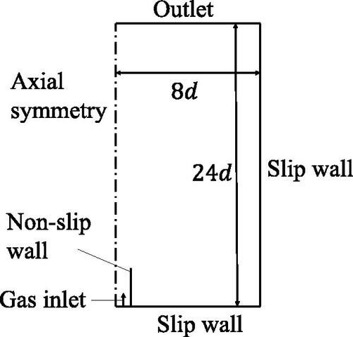
Table 6. Condition of calculation.

Nozzle diameter d	$1.7\mathrm{ }\mathrm{mm}$
Averaged velocity of gas U	$0.0881\mathrm{ }\mathrm{m}/\mathrm{s}$
Liquid viscosity	$0.126\mathrm{Pa}\cdot \mathrm{s}$
Liquid density	$1223.8\mathrm{kg}/{\mathrm{m}}^3$
Gas viscosity	$1.822\times {10}^{-5}\mathrm{ }\mathrm{Pa}\cdot \mathrm{s}$
Gas density	$1.205\mathrm{kg}/{\mathrm{m}}^3$
Surface tension coefficient	$6.6\times {10}^{-2}\mathrm{ }\mathrm{N}/\mathrm{m}$
Cell size	$0.03125\mathrm{ }\mathrm{m}$

Figure 10 shows the comparison bubbles’ behavior with that in Ohta et al. (2011). $T$ is the dimensionless time with time $t,$ an averaged velocity $U,$ and nozzle diameter $d,$ i.e. $T=Ut/d.$ This indicates that the proposed method can reproduce similar behavior in the formation of the bubbles. The detail patterns are in the following:

Figure 10. A sequence of calculated bubble formations (left: CLSVOF by Ohta et al. (2011), right: Proposed method, $T$ is dimensionless time).

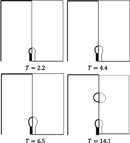
1. Bubble growth in the radial direction is similar

2. The timings of bubble growth and detachment are agreed upon

3. A leading bubble doesn’t affect a formation of a secondary bubble (Ohta et al. 2011).

4. Rising velocity of a leading bubble is agreed

Although the proposed method reduces the number of calculation procedures for level set function, good agreements can be obtained in the bubble dynamics.

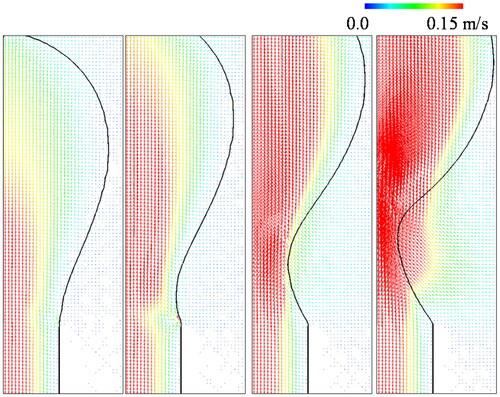
The simulation by Ohta et al. (2007) has a little difference in bubble volume of 4% from the experiment. In our calculation, the generated bubble is larger than that of Ohta et al. (2011). They pointed out that a slight difference in the timing of bubble breakup would give rise to large errors in the estimation of bubble volume. To confirm the effect, a sequence of pinch is shown in Figure 11. Ohta et al. (2011) and Albadawi et al. (2013) pointed out that gas velocity rapidly increases at the pinching of bubbles before detaching a bubble. The proposed method can obtain the same tendencies. However, the timing of the bubble breakup is slightly delayed under the order of 1 millisecond. Therefore, more flexible mesh refinement, especially at the pinching location is needed in future work.

Figure 11. A sequence of pinch-off.

The above-mentioned examples demonstrate that the proposed method can extensively improve the estimated precision of surface tension force, even though the method has a simple interface construction algorithm as with the method of Albadawi et al. (2013). In the future, more practical investigations including challenging problems with a dynamic contact angle and with interface behavior at high flow-rate regimes are needed.

4. Conclusion

A new method for converting the volume fraction $\alpha$ to the level set function $\varphi$ was proposed in this study. This method makes the calculation of $\varphi$ easier than the conventional CLSVOF method, and the precision of surface tension can be improved by the application of $\varphi .$ From two validation computations, we were able to obtain the following results:

1. The proposed method achieves a higher reconstruction accuracy for $\varphi$ than that of the existing simple coupled method because this method takes into account multi-dimensional profiles of $\alpha .$

2. If a surface tension evaluated by the proposed method is used in the computation, spurious currents can be considerably reduced.

3. The proposed method can simulate complex bubble motion including growth and detachment with the same degree of accuracy as the rigorous CLSVOF method.

Appendix

The ALE-like scheme in the Blackbill et al. (1992) is written as ($f=\alpha \text{ or }\varphi$): (32) $${\kappa }_{i,j}=-{\left(\nabla \cdot {\mathit{n}}_f\right)}_{i,j}=-{\left(\frac{\partial n_{fx}}{\partial x}+\frac{\partial n_{fy}}{\partial y}\right)}_{i,j}$$(32) (33) $${\left(\frac{\partial n_{fx}}{\partial x}\right)}_{i,j}=\frac{n_{fx,i+\frac{1}{2},j}-n_{fx,i-\frac{1}{2},j}}{\mathrm{\Delta }x}$$(33) (34) $${\left(\frac{\partial n_{fy}}{\partial y}\right)}_{i,j}=\frac{n_{fy,i,j+\frac{1}{2}}-n_{fy,i,j-\frac{1}{2}}}{\mathrm{\Delta }y}$$(34) (35) $$n_{fx,i+\frac{1}{2},j}=\frac{1}{2}\left(n_{fx,i+\frac{1}{2},j+\frac{1}{2}}+n_{fx,i+\frac{1}{2},j-\frac{1}{2}}\right)$$(35) (36) $$n_{fy,i,j+\frac{1}{2}}=\frac{1}{2}\left(n_{fy,i+\frac{1}{2},j+\frac{1}{2}}+n_{fy,i-\frac{1}{2},j+\frac{1}{2}}\right)$$(36) (37) $$n_{fx,i+\frac{1}{2},j+\frac{1}{2}}=\frac{{\left(\frac{\partial f}{\partial x}\right)}_{i+\frac{1}{2},j+\frac{1}{2}}}{\sqrt{{\left(\frac{\partial f}{\partial x}\right)}_{i+\frac{1}{2},j+\frac{1}{2}}^2+{\left(\frac{\partial f}{\partial y}\right)}_{i+\frac{1}{2},j+\frac{1}{2}}^2}}$$(37) (38) $${\left(\frac{\partial f}{\partial x}\right)}_{i+\frac{1}{2},j+\frac{1}{2}}=\frac{f_{i+1,j}+f_{i+1,j+1}-f_{i,j}-f_{i,j+1}}{2\mathrm{\Delta }x}$$(38) (39) $${\left(\frac{\partial f}{\partial y}\right)}_{i+\frac{1}{2},j+\frac{1}{2}}=\frac{f_{i,j+1}+f_{i+1,j+1}-f_{i,j}-f_{i+1,j}}{2\mathrm{\Delta }y}$$(39)

References

- Albadawi A, Donoghue DB, Robinson AJ, Murray DB, Delauré YMC. 2013. Influence of surface tension implementation in volume of fluid and coupled volume of fluid with level set methods for bubble growth and detachment. Int J Multiphase Flow. 53:11–28. doi: 10.1016/j.ijmultiphaseflow.2013.01.005
- Brackbill JU, Kothe DB, Zemach C. 1992. A continuum method for modeling surface tension. J Comput Phys. 100:335–354. doi: 10.1016/0021-9991(92)90240-Y
- Dhar A, Shimada N, Tomiyama A. 2013. A simple scheme for interface tracking. Kagaku Kogaku Ronbunshu. 39:86–93. doi: 10.1252/kakoronbunshu.39.86
- Dhar A, Shimada N, Hayashi K, Tomiyama A. 2014. An interface-capturing method for free-surface flows in a flow channel consisting of solid obstacles. J Chem Eng Japan. 47:230–240. doi: 10.1252/jcej.13we165
- Francois MM, Cummins SJ, Dendy ED, Kothe DB, Sicilian JM, Williams MW. 2006. A balanced-force algorithm for continuous and sharp interfacial surface tension models within a volume tracking framework. Comput Phys. 213:141–173. doi: 10.1016/j.jcp.2005.08.004
- Hayashi K. 2007. A study of numerical prediction method for two-phase flows based on an interfacial tracking model. [Doctoral Thesis]. Kobe University.
- Kunkelmann C, Stephan P. 2010. Modification and extension of standard volume-of-fluid solver for simulating boiling heat transfer. In V Europian Conference on Computational Fluid Dynamics,
- Lafaurie B, Nardone C, Scardovelli R, Zaleski S, Zanetti G. 1994. Modelling merging and fragmentation in multiphase flows with surfer. Comput Phys. 113:134–147. doi: 10.1006/jcph.1994.1123
- Losasso F, Fedkiw R, Osher S. 2006. Spatially adaptive techniques for level set methods and incompressible flow. Computer Fluids. 35:995–1010. doi: 10.1016/j.compfluid.2005.01.006
- Muzaferija S, Peric M, Sames P, Schelin T. 1998. A two-fluid navier-stokes solver to simulate water entry. Proc Twenty-Second Symposium on Na-Val Hydrodynamics
- Noh WF, Woodward PR. 1976. SLICK (Simple Line Interface Calculation). Lect Notes Phys. 59:330–360.
- Ohta M, Kikuchi D, Yoshida Y, Sussman M. 2007. Direct numerical simulation of the slow formation process of single bubbles in a viscous liquid. J Chem Eng Japan. 40:939–943. doi: 10.1252/jcej.06WE275
- Ohta M, Kikuchi D, Yoshida Y, Sussman M. 2011. Robust numerical analysis of the dynamic bubble formation process in a viscous liquid. Int J Multiphase Flow. 37:1059–1071. doi: 10.1016/j.ijmultiphaseflow.2011.05.012
- Olsson E, Kreiss G, Zahedi S. 2007. A conservative level set method for two phase flow ii. Comput Phys. 225:785–807. doi: 10.1016/j.jcp.2006.12.027
- Prosperitti A, Tryggvason G. 2009. Computational methods for multiphase flow. Cambridge: Cambridge University Press.
- Renardy Y, Renardy M. 2002. Prost: a parabolic reconstruction of surface tension for the volume-of-fluid method. Comput Phys. 183:400–421. doi: 10.1006/jcph.2002.7190
- Ubbink O, Issa RI. 1999. Method for capturing sharp fluid interfaces on arbitrary meshes. J Comput. Phys. 153:26–50. doi: 10.1006/jcph.1999.6276
- Xiao F, Honma Y, Kono T. 2005. A simple algebraic interface capturing scheme using hyperbolic tangent function. Int J Numer Meth Fluids. 48:1023–1040. doi: 10.1002/fld.975
- Yamamoto T, Okano Y, Dost S. 2017. Validation of S-CLSVOF method with the density-scaled balanced continuum surface force model in multiphase systems coupled with thermocapilary flows. Int J Numer Meth Fluids. 83:223–244. doi: 10.1002/fld.4267
- Yokoi K. 2007. Efficient implementation of THINC scheme: a simple and practical smoothed VOF algorithm. J Comput Phys. 226:1985–2002. doi: 10.1016/j.jcp.2007.06.020
- Youngs DL. 1982. Time-dependent multi-material flow with large fluid distortion. In Numerical Methods Fluid Dynamics, 273–285. New York: Academic Press.