Fast Prediction of Heat Flux Distribution in Boilers Using Computational Fluid Dynamics Simulation Data via Multi-Extreme Learning Machines

Abstract

The heat transfer and hydrodynamic safety of the water-cooled wall in coal-fired boilers are important guarantees for the safe and stable operation of thermal power units. In recent years, influenced by coal quality changes and load fluctuation, the ash deposition and slagging of the water wall and the fluctuation of heat load bring great challenges to the furnace heat transfer safety. It is urgent to monitor the heat flux distribution of the water-cooled wall in the furnace to ensure the safety of the heating surface. In this study, a calculation method for heat flux distribution of 350 MW boiler based on computational fluid dynamics (CFD) and extreme learning machine (ELM) is proposed. First, 120 typical operating conditions in boiler were simulated using ANSYS Fluent to characterize heat flux distribution. Next, to circumvent the high computational cost of CFD simulations, a heat flux distribution prediction model based on multi-ELM was developed by integrating the simulation data and the actual operating parameters of the boiler. Two parameters, namely, separated over-fire air (SOFA) damper opening and main burner secondary air damper opening, were applied to divide the 120 operating conditions into six categories, and use K-means algorithm to find the central operating condition of each category. In each category, the heat flux data of a specific operating condition were randomly selected as the verification set, and the validity of the heat flux distribution prediction models was verified. Finally, the prediction models of heat flux distribution based on multi-ELM were compared with the prediction models based on four contemporary neural network algorithms. Results showed that for the multi-ELM model, the prediction error was <10%, showing that it can accurately predict the heat flux distribution of a boiler and provide guidance for the regulation of the actual production process.

Keywords:

• Supercritical boiler
• Heat flux
• Computational fluid dynamics
• Extreme learning machine

1. Introduction

With the large-scale grid integration of renewable energy, the tasks of peak regulation and ensuring basic power supply for thermal power units have become increasingly demanding. Deep load regulation requires frequent and rapid load changes, which can lead to problems such as fouling and slagging in the furnace, furnace stress deformation and uneven heat transfer. The above issues can lead to a decrease in the heat transfer efficiency of water-cooled walls and even result in safety accidents like water-cooled wall rupture, thereby reducing the operational efficiency of the power unit and jeopardizing the safety of the power plant. The distribution of boiler heat flux is an important indicator for evaluating the heat dissipation performance of the furnace (Hao et al. 2019). Timely acquisition of boiler water-cooled wall heat flux distribution is important for boiler commissioning and safe operation.

Currently, the heat flux can be directly measured by installing heat flux measurement devices on the surface or inside the furnace (Anson and Godridge 1967; Gardon 1960; Godefroy et al. 1990; Ploteau et al. 2007). However, the direct measurement method is limited by the number of measurement devices and installation difficulties, which can only obtain heat flux values at a few points in the furnace, making it difficult to obtain the three-dimensional distribution of heat flux.

With the continuous advancement of computer technology, computational fluid dynamics (CFD) has been widely applied in boiler combustion simulation, including gas–solid flow (Li et al. 2018; Sun et al. 2019), combustion and NOx emissions (Du et al. 2017; Li et al. 2017; Tan et al. 2017; Zhang et al. 2015). Wang et al. (2020) comprehensively described the heat transfer estimation technology in the three-dimensional CFD model of coal-fired boilers, proposed a set of heat transfer sub-models that can be easily used to solve and analyze the practical problems of large boilers, and focused on the heat transfer calculation of the furnace water wall. Xu et al. (2016) utilized numerical simulation to determine gas–solid flow behavior in a massive circulating fluidized bed (CFB) boiler. The heat flux distribution was determined using the rate of heat transfer obtained from the cluster refresh model and the thermal–hydraulic coupled study. Zhang et al. (2016) carried out numerical simulations on the heat flux distribution of a barrier wall of a 600 MW supercritical arch-fired boiler (SC-AFB) under a variety of operating conditions. The experimental results show that the predicted heat flux distribution trend and value are in good agreement with the measured data. Numerical simulation of the heat flux distribution in boiler water-cooled wall using CFD techniques is a stable and highly accurate method. Due to the complex structure of the boiler furnace and the presence of hundreds of physical, chemical, and heat transfer reactions, using CFD numerical simulation can result in long computation periods. Based on the reasons mentioned above, it is challenging to obtain real-time information on the heat flux distribution of the boiler water-cooled wall through CFD numerical simulation. CFD is often used for offline numerical simulations in thermal power plants, and the experience gained from these simulations is then used to guide subsequent combustion control.

At present, the artificial intelligence modeling method based on big data has been successfully applied in the prediction of key parameters of boiler. Through artificial intelligence algorithms, complex nonlinear relationships between various input variables (such as temperature, pressure, etc.) and output variables (such as combustion efficiency, pollutant emissions concentration, etc.) in boiler systems can be accurately captured. Leiprecht et al. (2021) used data-driven methods to predict the heat load in district heating and refrigeration applications. Żymełka and Szega (2021) presented an artificial neural network-based prediction model for regional heating demands. Tang and Zhang (2019) proposed a deep belief network (DBN)-based technique for modeling combustion efficiency as well as NOx emissions. Wu et al. (2022) proposed a nonlinear dynamic soft measurement algorithm based on long short-term memory (LSTM) and least absolute convergence and selection operator (LASSO) for the nitrogen oxide (NOx) emissions of a power plant denitrification system. Li et al. (2023) proposed a novel combined model based on 1D semi-empirical model and three black box models to predict the dynamics of NOx emission of a 350 MW CFB boiler. Based on the inspiration of the above research, it is possible to use data-driven modeling methods to establish a nonlinear mapping relationship between numerical simulation data of boiler heat flux and key operational parameters, enabling the prediction of heat flux.

This study establishes a data-driven prediction model based on CFD numerical simulation data to overcome the long computation time of CFD simulations and achieve the rapid prediction of the three-dimensional distribution of heat flux on the boiler water-cooled wall.

The main content of this paper include three aspects:

1. The boiler combustion was simulated using ANSYS Fluent software, and numerical simulations of heat flux were obtained under 120 operating conditions.

2. According to the opening degree of the secondary air damper and the separated over-fire air (SOFA) damper, 120 operating conditions are divided into six categories, and the center operating condition was identified for each category to construct the modeling dataset.

3. A predictive model for the heat flux distribution on the furnace water-cooled wall based on ELM was established, enabling rapid three-dimensional prediction of heat flux.

Remainder of the paper is organized as follows. Section 2 introduces the 350 MW supercritical boiler used in the experiment and its CFD simulation. Section 3 presents the data processing before the experiment and experimental modeling. The experimental results and analyses are presented in Section 4. Finally, conclusions are presented.

2. CFD simulation of a 350 MW boiler

2.1. Description of the 350 MW coal-fired boiler

In this study, a 350 MW supercritical lignite boiler was investigated. The boiler has a π-type layout, with a single furnace, double flue at the tail, and a whole steel frame suspension structure. The dimensions of the furnace are 64.8 m high, 14.6273 m wide and 14.6273 m deep, with a tail rear flue depth of 6.82 m and a cold ash hopper elevation of 6.5 m. The main burner is a fixed type, consisting of two parts, upper and lower, with six layers of pulverized coal air chamber, four layers of separate combustion (SOFA) air chamber and eight layers of auxiliary air chamber. Each layer of pulverized coal air chamber has a total of four horizontal concentrated and light pulverized coal nozzles, and each layer of SOFA has four burner nozzles, of which the burner is mainly horizontal swing mode, which can not only adjust the center position of the flame in the furnace, but also adjust the flue temperature deviation of the furnace outlet caused by the combustion process; a total of four secondary air vents are arranged in each auxiliary air chamber. The final geometric model constructed from the study object is shown in Figure 1(a). The origin of the geometrical model is located at the center of the bottom of the furnace chamber.

Figure 1. 350 MW boiler: (a) geometry model; (b) boiler meshing.

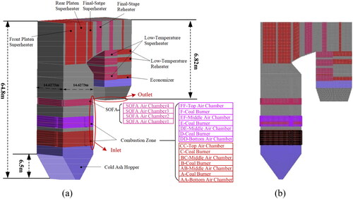
In addition, the water wall of the boiler is a membrane wall; the lower water wall and the ash hopper are equipped with spiral coils that ensure uniform heat absorption and small thermal deviation between tubes. Consequently, they are more suitable for the change of combustion conditions in the boiler. At an elevation of 43.232 m, the upper water wall is transformed into a vertical tube screen rising once, because of which, it can effectively compensate for the thermal deviation along the furnace perimeter.

2.2. Meshing and boundary condition setting in CFD

The CFD models proposed in this study are realized using ANSYS Fluent as the computing platform; the water wall is simplified as a furnace wall. The mesh division is mainly conducted by preprocessing software GAMBIT of Fluent, with the axes X, Y and Z indicating the furnace width, furnace height and furnace depth. The calculation areas are the cold ash hopper, lower burner, upper burner, SOFA, superheater, reheater and coal saver areas, which facilitate the generation of a suitable mesh. The calculation area is meshed using a mixed mesh to accommodate various complex geometric models, and the cold ash hopper area, superheater area, reheater area and coal saver area are meshed structurally. Due to the complex combustion conditions in the main combustion zone and SOFA zone, unstructured meshing and mesh encryption are applied to the area near the burner and nozzle for the accuracy of the simulation results and to better reflect the flow field changes. The mesh is constructed with 2,776,652 hexahedral structured cells. Figure 1 (b) shows the longitudinal section of the boiler.

The basic conservation equations for numerical simulation include the conservation of mass conservation of momentum, and conservation of energy. The combustion process of pulverized coal inside the boiler furnace satisfies these fundamental conservation equations. The specific mathematical formulas for these equations are shown below.

Mass conservation equation: (1) $$\frac{\partial \rho }{\partial t}+\frac{\partial }{\partial x_j}(\rho u_j)=0$$(1) where $\rho$ denotes fluid density; $t$ is the time; $u$ is the velocity vector; $\frac{\partial \rho }{\partial t}$ is the rate of mass transformation; $\frac{\partial }{\partial x_j}(\rho u_j)$ is the net outflow of mass.

Momentum conservation equation: (2) $$\begin{array}{c}\frac{\partial }{\partial t}(\rho u_i)+\frac{\partial }{\partial x_j}(\rho u_j{u}_i)=\frac{\partial {\tau }_{ij}}{\partial x_j}-\frac{\partial p}{\partial x_i}+\\ \rho g_i+F_i\end{array}$$(2) where $p$ denotes the static pressure, ${\tau }_{ij}$ is the stress tensor;$g_i$ and $F_i$ are the gravitational volumetric force and external volumetric force in the $i$ direction, respectively.

Energy conservation equation: The energy $E$ of a fluid is usually the sum of the internal energy $U,$ the kinetic energy $K=\frac{1}{2}{u}_i{}^2$ and the potential energy is $P.$ There is a relationship between the internal energy $U$ and the temperature $T,$ i.e., $U=c_{p}T.$ (3) $$\frac{\partial }{\partial t}(\rho T)+\frac{\partial }{\partial x_i}(\rho u_{i}T)=\frac{\partial }{\partial x_i}\left(\frac{k}{c_p}\frac{\partial T}{\partial x_i}\right)+S_T$$(3) where $c_p$ denotes specific heat capacity; $T$ is the temperature; $k$ is the heat transfer coefficient of the fluid; $S_T$ is the viscous dissipative term.

For the convenience of research, assume unchanged coal quality under different loads, without considering on-site temporary coal replacement and coal blending combustion. The parameters related to coal types involved in this study are shown in Tables 1 and 2. The coal particle size distribution follows the Rosin-Rammler distribution.

Table 1. Industrial analysis of coal quality.

Number	Name	Unit	Parameter values
1	Moisture M (received basis)	%	31.75
2	Ash A (received basis)	%	9.84
3	Volatile matter V (dry-ash-free)	%	42.42
4	Fixed carbon (received basis)	%	33.63
5	Low level heat generation Q (received basis)	kJ/kg	16,310

Table 2. Elemental analysis of coal quality.

Number	Name	Unit	Parameter values
1	Carbon C (received basis)	%	44.82
2	Hydrogen H (received basis)	%	2.68
3	Oxygen O (received basis)	%	10.26
4	Nitrogen N (received basis)	%	0.52
5	Sulphur S (received basis)	%	0.13

Based on the combustion mechanism analysis, select the combustion mechanism model in ANSYS Fluent. The realizable $k-\epsilon$ model predicts cylindrical jet problems more accurately, with high accuracy for flow separation and complex secondary flows. This model incorporates physical constraints in its derivation and modifications, which enables the model to better capture the characteristics of real turbulent flow. Therefore, the realizable $k-\epsilon$ model is used to compute fluid viscosity. For considering various factors such as scattering, local heat sources, and radiative heat transfer between gas and particles, the discrete ordinates (DO) model is employed to calculate thermal radiation. The species transport model to calculate flue gas components. The eddy dissipation concept model is chosen due to its ability to employ turbulent control of reaction rates, offering advantages such as high accuracy and broad applicability. As a result, the eddy dissipation concept model is utilized to calculate chemical reactions in turbulent processes. The combustion of coke is influenced by factors such as the oxygen diffusion rate on the coke surface and the chemical reaction rate. The kinetics/diffusion-limited combustion model can consider the effects of chemical reaction kinetics and heat and mass transfer. Therefore, the kinetics/diffusion-limited combustion model is used to simulate coke combustion. The boiler coal powder injection nozzle, secondary air inlet, and SOFA air inlet are set as "inlet" boundaries, and the economizer outlet is set as the "outlet" boundary. Using velocity as the gas-phase inlet, burner port is set to be 27 m/s, the secondary air inlet and the SOFA air inlet are set to 48 m/s; The pressure at the outlet is 0, and all wall surfaces are treated with standard wall function. The combustion process of the boiler was simulated using ANSYS Fluent software, and three-dimensional distribution data of boiler heat flux under different operating conditions were obtained. The data included the x, y, z coordinate values representing different positions on the furnace wall, along with their corresponding heat flux values.

The main boiler operating conditions used in the experiment include total air volume, total coal quantity, primary air flow, secondary air flow, SOFA damper opening, secondary air damper opening, temperature of secondary air and operation mode of coal mill. Using different arrangements and combinations, the heat flux data of 120 typical operating conditions are simulated, which can be used as the basis for establishing the heat flux model in the future. Among them, six pulverizers A–F operate in a certain combination, and the operation mode of pulverizers corresponds to the start-up mode of the A–F layer burners. According to the method described in the literature (Li et al. 2017), Eqs. (4)(4) $$x_r=\frac{H_r}{H_L}$$(4) and (5)(5) $$H_r=\frac{\sum n_i{B}_j{H}_{ri}}{\sum n_i{B}_i}$$(5) are used to convert different burner start-up modes into the height of the flame center inside the furnace. This conversion transforms discrete variables into continuous variables, which serve as inputs for the heat flux distribution prediction model. Boundary conditions, such as total air volume, total coal, and secondary air temperature, are set in accordance with the boiler’s practical operating parameters, as shown in Table 3. (4) $$x_r=\frac{H_r}{H_L}$$(4) (5) $$H_r=\frac{\sum n_i{B}_j{H}_{ri}}{\sum n_i{B}_i}$$(5) where $x_r$ indicates the relative height of the burner;$\mathrm{ }{H}_r$ is the arrangement height of the burner (i.e., the height from the bottom of the furnace or the middle plane of the cold ash hopper to the axis of the burner, m), calculated according to Eq. (5)(5) $$H_r=\frac{\sum n_i{B}_j{H}_{ri}}{\sum n_i{B}_i}$$(5) when several layers of burners are arranged;$\mathrm{ }{H}_L$ is the height of the furnace (i.e., from the bottom of the furnace or the middle plane of the cold ash hopper to the middle of the flue gas outlet of the furnace, m);$\mathrm{ }{n}_i$ is the number of burners in this layer;$\mathrm{ }{B}_i$ is the burning of coal for each layer of the burner; $H_{ri}$ is the arrangement height corresponding to each layer of burners.

Table 3. Description of numerical simulation boundary conditions.

Number	Operating parameters	Unit	Range
1	Load	MW	[175, 350]
2	Total air volume	t/h	[603, 1305]
3	Total coal	t/h	[90, 212]
4	Primary air flow	t/h	[218, 452]
5	Secondary air flow	t/h	[330, 897]
6	SOFA damper opening	%	[5, 100]
7	Secondary air damper opening	%	[10, 90]
8	Temperature of secondary air	°C	[320, 366]
9	Coal mill operation modes	–	ABCDEF/ABCDE/CDEF/BCDE/CDEF/CDE

2.3. Simulation results of heat flux

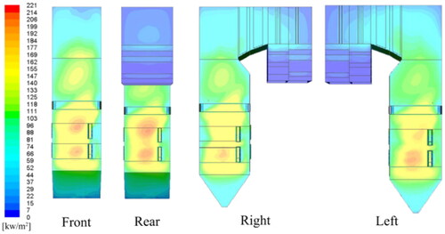
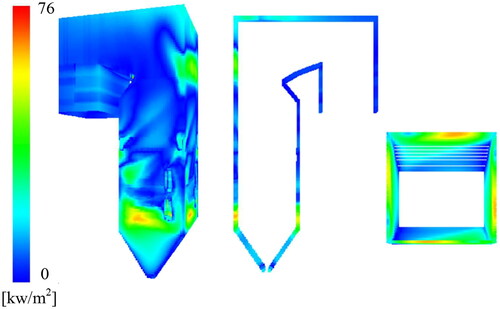
The water wall surface is simplified to the wall surface in the furnace, and the corresponding heat flux distribution under different operating conditions is obtained. The heat flux distribution of the boiler is closely related to the temperature distribution in the furnace. The area with high temperature inside the boiler also exhibits a high heat flux value on its surface. Figure 2 shows the simulation result of heat flux distribution over the entire boiler under a random operating condition. At the lower burner position in the boiler, during the early stages of combustion, the furnace temperature and heat flux density are relatively low. As the furnace position rises, the heat release from combustion increases, leading to a rapid increase in heat flux density on the boiler surface reaching its maximum value at the upper burner position. As the furnace position continues to move up, the furnace gas temperature decreases steadily and the heat flux decreases gradually.

Figure 2. Heat flux distribution of furnace wall.

3. ELM-based heat flux distribution prediction model

The heat flux value and its distribution in the water wall of the furnace cannot be measured because of the few measurement points. Moreover, CFD simulation takes a long time to quickly obtain the heat flux distribution. Therefore, a data-driven rapid modeling method of three-dimensional heat flux distribution is proposed. This method uses the heat flux value obtained by CFD simulation as the data support. To solve the problem of time-consuming and complex calculation in traditional CFD simulation, CFD simulation data are used with the data-driven prediction algorithm to develop a heat flux distribution prediction model for the water wall in the furnace. Figure 3 depicts the general technical flow chart of the heat flux distribution prediction model.

Figure 3. Framework of heat flux distribution fast prediction in boilers using computational fluid dynamics simulation data via multi-extreme learning machines.

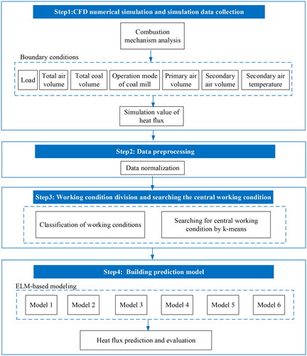
Step 1: Heat flux distribution based on main boiler operating conditions is simulated using ANSYS Fluent software. It provides a data basis for establishing the heat flux distribution model. The details of CFD are presented in Section 1.

Step 2: The simulation data are preprocessed to improve the convergence and computing speed of the deep learning process. In particular, to remove the impact of differing dimensions on modeling findings, the min–max method is used to normalize the data before modeling (Section 2.1).

Step 3: According to the damper opening of SOFA and secondary air, the CFD simulation data under all operating conditions are classified into six categories, and six sub-models are established. Before predicting the heat flux of unknown operating conditions, it is necessary to determine the sub-model to which the operating conditions belong. The k-means method is used to determine the central operating condition under each category to prevent large deviation of prediction results. The detailed principle is explained in Section 2.2.

Step 4: Take the actual on-site coal volume, air volume, wind temperature and other operating parameters and numerical simulation data as input, and take the heat flux value as output. Six sub-models for predicting the heat flux distribution in the furnace are established by using different algorithms. When predicting the heat flux of an unknown operating condition, first determine which category the operating condition belongs to according to the burndown damper opening and the secondary damper opening, and then use the corresponding sub-model to predict the heat flux distribution. At the same time, in each sub-model, the heat flux data of a specific operating condition are randomly selected as the validation set; to evaluate and examine the results, the multi-ELM-based models are compared to that of deep neural network (DNN), echo state network (ESN), DBN, and multilayer perceptron (MLP) models.

3.1. Data processing

When establishing the heat flux prediction model, there are great differences in the dimensions of different input variables. In order to eliminate the influence of dimensional differences on modeling accuracy, the minimum–maximum method is used to normalize the simulation data before the experiment starts. Thus, each value is mapped to a closed interval [0,1]. The core idea is that the output and input distribution of each layer of the neural network should be consistent to ensure that the data distribution between the layers is relatively stable and does not change, so as to avoid slow training speed and overfitting. Normalization is carried out using the following equation: (6) $$x_i^{\mathrm{*}}=\frac{x_i-x_{\min }}{x_{\max }-x_{\min }}$$(6) where $x_i$ is the simulation value of the parameter, $x_{\max }$ and $x_{\min }$ are the maximum and minimum value of the parameter, respectively, and $x_i^{*}$ is the normalized value.

3.2. Classification of operating conditions

The 120 operating conditions are arranged in a specific order and labeled T1–T120. However, direct modeling can result in large prediction biases. Therefore, the k-means clustering algorithm is used in each large class to find a central operating condition so that the Euclidean distance between this operating condition and other operating conditions under this operating condition category is the minimum sum of heat flux values. The distance calculation formula is shown in Eq. (7)(7) $$D=\sum {}_{j=1}^k\sqrt{{\sum }_{i=1}^n{(x_i-y_i)}^2}$$(7) . Table 4 shows the classification results of 120 operating conditions, and the "a" operating conditions marked in the table are the central operating condition of each type. (7) $$D=\sum {}_{j=1}^k\sqrt{{\sum }_{i=1}^n{(x_i-y_i)}^2}$$(7) where $k$ is the number of cluster centers, $x_i$ is the heat flux value under the central operating condition, $y_i$ is the heat flux value under the corresponding coordinates of other operating conditions, and $D$ is the sum of Euclidean distances between the heat flux of other operating conditions and the central operating condition.

Table 4. Classification of 120 operating conditions.

Types	SOFA dampers opening (#1–#4) (%)	Main burner secondary damper opening (%)	Classification of operating conditions
Category 1	100/100/100/100	70/70/70/70/70 /70/70/70	T1, T2, T10, T11, T12, T19, T20, T21, T56, T57, T65, T66^a, T74, T75, T110, T111, T119, T120, T3, T55
Category 2	100/100/100/100	90/90/60/60/60/60/40/40	T28, T29, T37, T38, T39, T46, T47, T48, T83, T84, T92, T93^a, T101, T102, T64, T73, T109, T118, T30, T82
Category 3	5/5/95/95	70/70/70/70/70 /70/70/70	T7, T8, T16, T17, T18, T25, T26, T27, T62, T63, T71, T72^a, T80, T81, T116, T117, T91, T100, T9, T61
Category 4	5/5/95/95	90/90/60/60/60/60/40/40	T34, T35, T43, T44, T45, T52, T53, T54, T89, T90^a, T98, T99, T107, T108, T70, T79, T115, T36, T88, T97
Category 5	5/95/95/5	70/70/70/70/70/70/70/70	T4, T5, T13, T14, T15, T22, T23, T24, T59, T60, T68, T69^a, T77, T78, T113, T114, T106, T6, T58, T67
Category 6	5/95/95/5	90/90/60/60/60/60/40/40	T31, T32, T40, T41, T42, T49, T50, T51, T86, T87, T95, T96^a, T104, T105, T76, T112, T33, T85, T94, T103

3.3. ELM-based prediction model

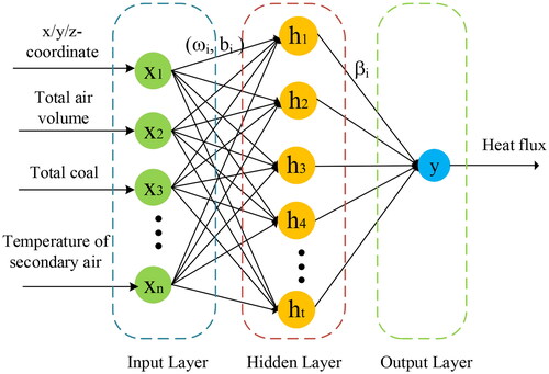
The extreme learning machine (ELM) is a single-hidden layer feed forward network (SLFN) solution algorithm. ELM has the advantages of fast learning, universality, and simple parameter setting, and it is frequently employed in several fields, such as regression (Li and Niu 2013), classification (Wang et al. 2012; Zheng et al. 2013), forecasting and diagnosis (Chen and Ou 2011; Xu et al. 2013), and so on. Figure 4 shows the structure block diagram of an ELM network. In this modelling, the ELM algorithm uses a tanh function with 25 implied layers and the dynamic parameters have been adjusted to give the best results at 0.02.

Figure 4. Structure of ELM network for prediction of heat flux distribution.

When predicting the heat flux of an unknown operating condition, the damper opening of SOFA and secondary air is measured to determine the sub-model to which the operating condition belongs, and then, the corresponding sub-model is used to predict the heat flux distribution. Of the 20 operating conditions, 17 are considered as the training set, 1 is used as the test set, and 1 is chosen randomly as the verification set to ensure model accuracy.

The multi-ELM-based prediction model for heat flux distribution in a furnace is expressed as in the following equation: (8) $$ht=f({IN}_{ht},\mathrm{ }{\omega }_i,\mathrm{ }{b}_i,{\beta }_i)$$(8) where $ht$ is the difference between the predicted heat flux value and the heat flux value under the central operating condition, ${IN}_{ht}$ is the input variable for predicting heat flux, ${\omega }_i$ is the weight between different layers in the ELM-based heat flux distribution prediction model, $b_i$ is the offset of the model, and ${\beta }_i$ is the output weight.

4. Results and discussion

4.1. Evaluation of experimental results

CFD simulation data are obtained using ANSYS Fluent software on a system with following parameters: the HP Z840 with Intel Xeon E5-2650V3 processor, 64 GB DDR4 memory and 4000 G hard drive. It takes about 14 days for one operating condition of a computing cycle. Modeling is carried out using python in Dell Inspiron 5447 with 4th generation Core i5-4210U dual-core processor with 8 G RAM in Windows 10.

R², mean absolute error (MAE), and mean absolute percentage error (MAPE) are employed as indicators to evaluate the performance of the generalization capacity and prediction performance of the model. The closer the R² is to 1, the higher the fitting degree of the model predicted value and the simulation value. Smaller MAE and MAPE values indicate higher prediction accuracy of the model. To more intuitively see the results of heat flux under each model, the mean MAE (MMAE) values of all predicted operating conditions are calculated and compared. The calculation formulas are given in Eqs. (9)–(12). (9) $$R^2=1-\frac{{\sum }_i{({\widehat{y}}_i-y_i)}^2}{{\sum }_i{({\widehat{y}}_i-{\overline{y}}_i)}^2}$$(9) (10) $$\mathrm{MAE}=\frac{1}{n}{\sum }_{i=1}^n\left|y_i-{\widehat{y}}_i\right|$$(10) (11) $$\mathrm{MAPE}=\frac{1}{n}\sum _i\frac{\left|{\widehat{y}}_i-y_i\right|}{y_i}\times 100\%$$(11) (12) $$\mathrm{MMAE}=\frac{1}{m}\times {\sum }_{i=1}^m\frac{{\sum }_{i=1}^n\left|y_i-{\widehat{y}}_i\right|}{n}$$(12) where ${\widehat{y}}_i$ is the predicted value of the heat flux distribution model, $y_i$ is the simulation value of the parameter, ${\overline{y}}_i$ is the average value of simulation value, and $m$ is the number of predicted operating conditions.

4.2. Prediction performance of ELM-based models

During the modeling of the six models, each model was trained and tested 19 times, and Table 5 shows the corresponding MMAE values, which are all within 10% of the range of variation of the heat flux values, indicating that the prediction results of the models are highly accurate.

Table 5. MMAE values of the six prediction models.

Model	MMAE	Model	MMAE
Model 1	13.40748	Model 4	15.04892
Model 2	13.11218	Model 5	15.00983
Model 3	14.36336	Model 6	14.21825

The MAE value for predicting heat flux density under the randomly selected operating condition T10 is 11.8623. The absolute error values of the predicted and simulated values of the corresponding ELM-based model are shown in Figure 5. It can be seen from the figure that there is a relatively large error in some regions of the burner. This is due to the rapid change of velocity field in the middle of the furnace and near the side walls, the existence of squeezing effect of the airflow, and the non-uniform distribution of heat flux in the water-cooled wall, which leads to a large prediction error of the model. However, most of the regions in the prediction error plots show dark blue or light blue colours, indicating that the ELM-based model has a low prediction error. Therefore, the modeling method proposed in this paper can meet the accuracy of predicting the heat flux distribution of the water wall of coal-fired boilers in power plants.

Figure 5. Prediction error distribution of T10 operating condition.

4.3. Comparative analysis of different algorithms in six models

To further verify the performance of the ELM based model, DNN (Dan et al. 2012), ESN (Jaeger 2001), DBN (Hinton et al. 2006), and MLP (Rumelhart et al. 1986) models were built for comparison using the same training and test samples. The hyperparameter settings of the comparison model are shown in Table 6. Figure 6 compares the heat flux density prediction results of the six types of models under any random operating condition using five different algorithms. All five algorithms demonstrate excellent ability to forecast the heat flux in the furnace, but in comparison, the change trends of prediction results obtained by the ELM-based model are closer to the change trends of the simulated values, which indicates that the ELM-based heat flux distribution prediction model has better fitting effect and prediction ability.

Figure 6. Comparison of prediction results with different algorithms under different operating conditions.

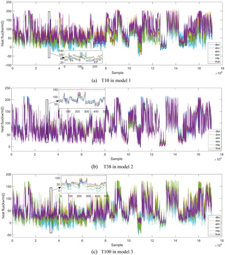
Table 6. The hyperparameter settings of the comparison model.

Model	Parameters	Value
DNN	Number of hidden layers	3
	Number of neurons	45:60:50
	Activation functions	relu:tanh:relu
	Learning rate	0.1
	Optimizer	sgd
DBN	Number of hidden layers	3
	Number of neurons	52:60:50
	Activation functions	relu:relu:relu
	Learning rate	0.08
	Optimizer	Adam
ESN	Reservoir size	50
	Spectral radius	0.88
	Leaking_rate	0.2
	Regularization coefficient	1.0 × 10^–6
	Input scaling	1.25
MLP	Number of hidden layers	3
	Number of neurons	50:60:50
	Activation functions	relu:relu:tanh
	Learning rate	0.2
	Optimizer	sgd

Table 7 shows the results of heat flux distribution prediction models under various operating conditions to further analyze the prediction accuracy of each algorithm. Except for the T87 operating condition in prediction model 6, the evaluation indexes of the predicted values of the ELM-based prediction model are better than those of the remaining four models. Among the six models, the R² of the ELM-based prediction model is maintained at approximately 0.9, showing good fit of the prediction model with the simulation values; compared with the other four algorithmic models, the MAE values of the ELM-based prediction model are the smallest among the six models, and most of its MAPE values are also within 20%, reflecting that the ELM-based prediction model has better prediction accuracy and generalization ability. More importantly, the modelling time for the elm-based prediction model is much less than that of the other four algorithmic models, saving a significant amount of time for heat flux distribution prediction. Figure 7 shows the display of 3D simulation results using different modeling algorithms under T10 operating condition, and it can be seen from the heat flux distribution in the figure that the results of the ELM algorithm are the closest to the real simulation results.

Figure 7. 3D simulation results of different modeling algorithms under T10 operating condition.

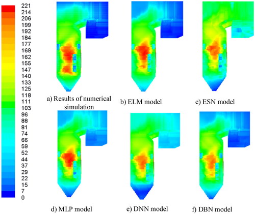
Table 7. Comparison of experimental results with different algorithms.

Predicted operating conditions	Experiment evaluation	ELM	DNN	DBN	ESN	MLP
T10 in model 1	TIME	69.3587^a	1056.4089	2266.1512	141.3149	519.2491
	R^2	0.8714^a	0.5424	0.2320	0.0176	0.2972
	MAE	11.8623^a	21.9845	30.7919	37.5130	30.4623
	MAPE (%)	17.4651^a	114.2546	196.2597	421.3746	196.01334
T38 in model 2	TIME	59.7173^a	682.3446	1475.6667	129.6851	380.5857
	R^2	0.9579^a	0.9429	0.9288	0.9103	0.9215
	MAE	7.6149^a	7.9153	9.0539	9.5711	9.7472
	MAPE (%)	11.7745^a	13.2729	14.0125	13.9288	14.6031
T100 in model 3	TIME	88.6658^a	382.4942	1580.1579	119.4647	481.1813
	R^2	0.9259^a	0.8969	0.7909	0.7758	0.8576
	MAE	7.9075^a	10.8123	15.7662	17.2519	13.6495
	MAPE (%)	82.4939^a	231.5923	115.5787	365.7249	239.8661
T107 in model 4	TIME	97.0809^a	555.6525	1951.2991	119.4607	423.2518
	R^2	0.9585^a	0.9357	0.8743	0.8326	0.9231
	MAE	6.6653^a	8.7424	11.9125	13.2840	9.4442
	MAPE (%)	34.9293^a	70.8032	54.04315	34.6159	92.8160
T13 in model 5	TIME	97.7081^a	488.8246	1553.7756	119.2566	355.7072
	R^2	0.9367^a	0.8847	0.8701	0.7636	0.8643
	MAE	9.1899^a	11.6289	13.1962	16.7540	12.8919
	MAPE (%)	12.0248^a	16.3099	16.6245	20.9785	16.7410
T87 in model 6	TIME	79.1138^a	556.7297	1701.8544	99.6779	323.8292
	R^2	0.9875^a	0.9821	0.9510	0.9400	0.9746
	MAE	3.1317^a	4.4273	8.0488	9.5193	5.1519
	MAPE (%)	16.0667	10.3511^a	27.2567	65.5657	14.1892

^a Good experimental results.

4.4. Comparative experiments of different loads under the same model

To test the performance of the modeling method, this section adjusts the data set to verify the prediction performance and popularization performance of the heat flux distribution prediction model under different boiler operation conditions. Taking model 2 as an example, the heat flux of T38 operating condition at 100% unit load is predicted in Section 3.3, and five algorithms are used to compare the experiments for T84 operating condition at 75% load and T82 operating condition at 50% load. The experimental outcomes are presented in Figure 8. As shown in Figures 6(b) and 8, for all algorithmic models, the projected and simulated value curves for estimating heat flux under various loads show the same trend, but the ELM-based model has a better fit. Table 8 shows a comparison of the specific experimental results, and the best results of different prediction algorithms have been marked with “a” in Table 8. Overall, most evaluation indexes of the ELM-based model are better than those of the other algorithmic models. However, under the T82 operating condition, the MAPE value for heat flux prediction is relatively high, indicating that the model has a significant deviation in predicting the heat flux values at 50% load. The prediction performance of heat flux density varies with different algorithms, but the predicted heat flux density distribution patterns are generally consistent with the distribution patterns of simulated heat flux density values.

Figure 8. Prediction results with different algorithms under different loads.

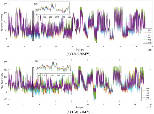
Table 8. Model evaluation with different algorithms under different loads.

Operating conditions	Evaluation indicators	ELM	DNN	DBN	ESN	MLP
	R^2	0.9579^a	0.9429	0.9288	0.9103	0.9215
T38 in 350 MW	MAE	7.6149^a	7.9153	9.0539	9.5711	9.7472
	MAPE (%)	11.7745^a	13.2729	14.0125	13.9288	14.6031
T84 in 260 MW	R^2	0.9766	0.9825^a	0.9662	0.9476	0.9474
	MAE	4.6330	3.9694^a	6.1628	7.3804	7.4160
	MAPE (%)	13.6392^a	22.4551	22.7794	26.8628	57.6548
T82 in 175 MW	R^2	0.9393^a	0.8916	0.7825	0.7704	0.8466
	MAE	7.0011^a	10.6619	14.7455	16.7826	12.9285
	MAPE (%)	72.6287^a	170.4378	76.8143	169.5044	133.9807

5. Conclusions

In view of the fact that the number of boiler temperature measurement point is small, the heat flux distribution of the furnace water wall cannot be measured, and it takes a long time to obtain the heat flux distribution of the furnace water wall through CFD numerical simulation. A data-driven fast modeling method for three-dimensional heat flux distribution is proposed. The method determines the boundary conditions of the numerical simulation according to the actual operating parameters of the boiler, and the numerical simulation is carried out for 120 different operating conditions using FLUENT software to obtain the simulated values of heat flux during steady-state operation of the furnace chamber. The 120 operating conditions were categorized according to SOFA damper opening and main burner secondary damper opening. For each category, the k-means algorithm was used to determine the central operating condition and build different prediction models. The prediction models of furnace heat flux distribution were established using ELM, DNN, DBN, ESN and MLP based algorithms. Through the comparative analysis of experimental results, the heat flux distribution prediction model based on ELM algorithm has high prediction accuracy and better fitting effect. In addition, by combining simulation data with modeling, the prediction time of heat flux distribution is greatly shortened, and the combustion situation can be determined in real time, which provides an important reference for timely adjustment of actual operation parameters. Due to the complexity of the boiler combustion process, even though the actual operating conditions are used as the boundary conditions for CFD simulation, the heat flux values obtained by numerical simulation still have some deviations from the actual boiler combustion operating conditions. In the future, in order to better describe the real-time heat flux distribution, the heat flux values obtained from the modeling in this paper can be corrected according to the values of the temperature and other parameters at the actual field measurement points of the boiler.

Disclosure statement

No potential conflict of interest was reported by the author(s).

References

- Anson D, Godridge AM. 1967. A simple method for measuring heat flux. J Sci Instrum. 44:541–544. doi: 10.1088/0950-7671/44/7/313.
- Chen FL, Ou TY. 2011. Sales forecasting system based on Gray extreme learning machine with Taguchi method in retail industry. Expert Syst Appl. 38:1336–1345. doi: 10.1016/j.eswa.2010.07.014.
- Dan C, Ueli M, Jonathan M. 2012. Multi-column deep neural network for traffic sign classification. Neural Netw. 32:333–338.
- Du Y, Wang C, Lv Q, Li D, Liu H, Che D. 2017. CFD investigation on combustion and NOx emission characteristics in a 600 MW wall-fired boiler under high temperature and strong reducing atmosphere. Appl Therm Eng. 126:407–418. doi: 10.1016/j.applthermaleng.2017.07.147.
- Gardon R. 1960. A transducer for the measurement of heat flow rate. J Heat Transfer. 82:396–398. doi: 10.1115/1.3679968.
- Godefroy JC, Clery M, Gageant C, Francois D, Servouze Y. 1990. Thin film temperature heat fluxmeters. Thin Solid Films. 193–194:924–934. doi: 10.1016/0040-6090(90)90246-A.
- Hao X, Xu P, Ma D. 2019. Analysis of hydrodynamic characteristics in water wall of supercritical boiler. J Eng Thermophys. 40:2334–2339.
- Hinton GE, Osindero S, Teh Y-W. 2006. A fast learning algorithm for deep belief nets. Neural Comput. 18:1527–1554. doi: 10.1162/neco.2006.18.7.1527.
- Jaeger H. 2001. The “echo state” approach to analysing and training recurrent neural networks-with an erratum note. Vol. 148. Bonn, Germany: German National Research Center for Information Technology GMD Technical Report. p. 13.
- Leiprecht S, Behrens F, Faber T, Finkenrath M. 2021. A comprehensive thermal load forecasting analysis based on machine learning algorithms. Energy Rep. 7:319–326. doi: 10.1016/j.egyr.2021.08.140.
- Li G, Niu P. 2013. An enhanced extreme learning machine based on ridge regression for regression. Neural Comput Appl. 22:803–810. doi: 10.1007/s00521-011-0771-7.
- Li J, Yan S, Liu Y. 2017. Boiler course design guide. 2nd ed. Beijing (China): Electric Power Press. p. 28–29.
- Li S, Chen Z, He E, Jiang B, Li Z, Wang Q. 2017. Combustion characteristics and NOx formation of a retrofitted low-volatile coal-fired 330 MW utility boiler under various loads with deep-air-staging. Appl Therm Eng. 110:223–233. doi: 10.1016/j.applthermaleng.2016.08.159.
- Li S, Ma S, Wang F. 2023. A combined NOx emission prediction model based on semi-empirical model and black box models. Energy. 264:126130. doi: 10.1016/j.energy.2022.126130.
- Li Z, Miao Z, Zhou Y, Wen S, Li J. 2018. Influence of increased primary air ratio on boiler performance in a 660 MW brown coal boiler. Energy. 152:804–817. doi: 10.1016/j.energy.2018.04.001.
- Ploteau JP, Glouannec P, Noel H. 2007. Conception of thermoelectric flux meters for infrared radiation measurements in industrial furnaces. Appl Therm Eng. 27:674–681. doi: 10.1016/j.applthermaleng.2006.05.010.
- Rumelhart DE, Hinton GE, Williams RJ. 1986. Learning representations by back-propagating errors. Nature. 323:533–536. doi: 10.1038/323533a0.
- Sun W, Zhong W, Echekki T. 2019. Large eddy simulation of the interactions between gas and particles in a turbulent corner-injected flow. Adv Powder Technol. 30:2139–2149. doi: 10.1016/j.apt.2019.06.029.
- Tan P, Tian D, Fang Q, Ma L, Zhang C, Chen G, Zhong L, Zhang H. 2017. Effects of burner tilt angle on the combustion and NOx emission characteristics of a 700 MWe deep-air-staged tangentially pulverized-coal-fired boiler. Fuel. 196:314–324. doi: 10.1016/j.fuel.2017.02.009.
- Tang Z, Zhang Z. 2019. The multi-objective optimization of combustion system operations based on deep data-driven models. Energy. 182:37–47. doi: 10.1016/j.energy.2019.06.051.
- Wang B, Wang G, Li J, Wang B. 2012. Update strategy based on region classification using ELM for mobile object index. Soft Comput. 16:1607–1615. doi: 10.1007/s00500-012-0821-9.
- Wang H, Zhang C, Liu X. 2020. Heat transfer calculation methods in three-dimensional CFD model for pulverized coal-fired boilers. Appl Therm Eng. 166:114633. doi: 10.1016/j.applthermaleng.2019.114633.
- Wu X, Yu X, Xu R, Cao M, Sun K. 2022. Nonlinear dynamic soft-sensing modeling of NOx emission of a selective catalytic reduction denitration system. IEEE Trans Instrum Meas. 71:1–11. doi: 10.1109/TIM.2022.3141154.
- Xu L, Cheng L, Cai Y, Liu Y, Wang Q, Luo Z, Ni M. 2016. Heat flux determination based on the waterwall and gas–solid flow in a supercritical CFB boiler. Appl Therm Eng. 99:703–712. doi: 10.1016/j.applthermaleng.2016.01.109.
- Xu Y, Dai Y, Dong Z, Zhang R, Meng K. 2013. Extreme learning machine-based predictor for real-time frequency stability assessment of electric power systems. IET Gen Transm Distrib. 7:391–397.
- Zhang D, Meng C, Zhang H, Liu P, Li Z, Wu Y, Lu J, Zhou W, Ran S, Zhang D. 2016. Studies on heat flux distribution on the membrane walls in a 600 MW supercritical arch-fired boiler. Appl Therm Eng. 103:264–273. doi: 10.1016/j.applthermaleng.2016.04.114.
- Zhang X, Zhou J, Sun S, Sun R, Qin M. 2015. Numerical investigation of low NOx combustion strategies in tangentially-fired coal boilers. Fuel. 142:215–221. doi: 10.1016/j.fuel.2014.11.026.
- Zheng W, Qian Y, Lu H. 2013. Text categorization based on regularization extreme learning machine. Neural Comput Appl. 22:447–456. doi: 10.1007/s00521-011-0808-y.
- Żymełka P, Szega M. 2021. Short-term scheduling of gas-fired CHP plant with thermal storage using optimization algorithm and forecasting models. Energ Convers Manage. 231:113860–113874. doi: 10.1016/j.enconman.2021.113860.