Efficiency and Status in Polygynous Pastoralist Households

Abstract

Decision-making structures may be different across polygynous and monogamous households, leading to different economic outcomes and requiring different targeting of anti-poverty programmes. We study efficiency in semi-nomadic pastoralist households in Northern Senegal with lab-in-the-field games. We find that monogamous and polygynous families are equally productively inefficient overall. However, average contributions at the household level mask differences across dyads. Junior wives receive less but give more to their husbands than senior wives, leaving junior wives worse off than other household members.

1. Introduction

Polygynous¹ families have often been overlooked by the household literature. Most theoretical models assume only two decision-makers and empirical work often ignores or excludes multi-member marriages. Household decision-making is likely different in polygynous families because discussion occurs not only between the husband and each wife but also between co-wives, with each wife having a different position of power. Given that polygyny is common in Sub-Saharan Africa – with an estimated one in four women being in a polygynous union (Arthi & Fenske, 2018) – understanding decision-making dynamics in polygynous households is important not only for understanding inefficiencies that may or may not occur but also for adjusting how anti-poverty programmes are targeted to individuals within households.

The presence of additional wives increases the complexity of intra-household decision-making and opens the possibility of both cohesion and friction in interpersonal dynamics. On the one hand, economies of scale and labour-sharing in domestic production could induce co-wives to collaborate with one another. The potential for polygyny to be productivity-enhancing was proposed by Boserup (1970) who posited co-wife cooperation for division of both household tasks and agricultural labour as a reason for the existence of polygyny and its prevalence.² On the other hand, there may be diminishing returns to polygamy since the husband or land is fixed (Becker, 1991). Moreover rivalry for resources and affection could lead to rifts and lower collaboration.

The existing evidence in the lab and field does not agree on whether polygynous families are more collaborative or efficient than monogamous families. Across co-wives, the anthropological literature mainly reports conflict and competition (Jankowiak, Sudakov, & Wilreker, 2005; Kazianga & Klonner, 2009) and associational studies find that women in polygynous households have lower quality physical and mental health (Bove & Valeggia, 2009; Hadley, 2005; Shepard, 2013), as do their children (Amey, 2002; Sellen, 1999; Wagner & Rieger, 2015). This is consistent with Rossi (2019), who finds that co-wives strategically raise their fertility to compete with one another for resources. However, Akresh, Chen, and Moore (2016) find smaller gender gaps in agricultural production in polygynous families compared to monogamous families in Burkina Faso, while Damon and McCarthy (2019) find higher yields in polygynous families than monogamous in Tanzania, suggesting that polygynous families in some cases are similarly or more efficient than their monogamous counterparts. In the lab, Barr, Dekker, Janssens, Kebede, and Kramer (2019) find that polygynous spouses contribute less in a public goods game than monogamous spouses in Western Nigeria, forgoing a substantial amount of income. In other words, polygynous spouses behave less efficiently than monogamous spouses. On the other hand, Munro, Kebede, Tarazona-Gomez, and Verschoor (2019) find that polygynous spouses in Northern Nigeria are no less (or more) efficient than monogamous spouses in a public goods game.³

Much of the existing literature on polygyny, however, focuses on crop farming households where traditionally women were an economic asset that helped expand household production. We contribute to the sparse literature by studying monogamous and polygynous households that are semi-nomadic pastoralist in Northern Senegal where cattle are the main productive asset, rather than land. We examine efficiency between husbands, wives, and co-wives using public goods games and find that monogamous and polygynous families are equally productively inefficient, with both types of families failing to maximise household income. However, there are important disparities in contribution rates by specific playing pairs in polygynous households. Junior wives contribute more to their husbands than do senior wives, but receive less from their husbands than senior wives. This finding is consistent with field evidence that suggests that junior wives suffer more domestic violence than senior wives (Hidrobo, Heath, & Roy, 2018) and the children of junior wives are less healthy (Gibson & Mace, 2007; Matz, 2016). Co-wives also contribute less to each other than to their husbands, suggesting competition rather than strategic cooperation across wives. Together, this leaves junior wives the worst off members of the household. This result suggest that policy makers should be especially thoughtful about reaching junior wives in polygynous households.

The paper proceeds as follows: Section 2 describes the experimental setting and design; Section 3 discusses descriptive statistics and sample selection; Section 4 presents our results; Section 5 concludes.

2. Experimental setting and design

2.1. Experimental setting

2.1.1. Polygyny in Senegal

Polygyny as an institution remains widespread in much of sub-Saharan Africa. The DHS Survey of Senegal in 2017 found that 32 per cent of women 15–49 years were in registered polygynous unions, and it is possible that additional customary polygynous unions remain unregistered. Polygynous families may form over time, and women in younger cohorts may eventually join polygynous households. In Antoine et al. (2002), it is estimated that roughly half of women in Senegal will be in a polygynous union at some point in their lives, which is consistent with the DHS data that show that 53 per cent of women 45–49 years old are in a polygynous union (ANSD and ICF, 2018).⁴ Polygyny is legal in Senegal, according to article 133 of the 1972 Family Code, and it is also legal according to Islamic religious codes. In Senegal a man may register a union as polygynous or monogamous when he gets married⁵ and may then take up to four wives. Analysing DHS data in Senegal and four other countries, Timaeus and Reynar (1998) show a woman is not likely to stay unmarried, whether widowed or divorced, for long, and she is more likely to enter a polygynous union after her first marriage dissolves. They also demonstrate that some polygynous unions arise through the levirate, that is, a man marrying his dead brother’s wife, or the sororate, a widower being obliged to marry a dead wife’s sister.

2.1.2. Study setting and design

The lab-in-the field games were conducted as part of a baseline survey for a dairy value chain study conducted in November 2014. The sample is composed of semi-nomadic dairy farmers who live near the town of Richard Toll and deliver milk to a local dairy processing company, La Laiterie du Berger. Households or members of the household move around with their cattle in search for pasture and water. Men are responsible for managing the household’s herd, while women are responsible for domestic chores and milking cows (Parisse, 2012). A companion study finds inefficiencies in milk production among this population, with male owned cows producing more milk than female owned cows (Hoel, Hidrobo, Bernard, & Ashour,2020).⁶

The respondents in our sample are Fulani with a patrilineal and patrilocal heritage, and polygyny is common. Households live in concessions that are composed of sub-nuclear families, many times consisting of three generations: a household head, his wives, his children, and their wives and children. Marriages are usually arranged and at the time of marriage, the new husband’s family traditionally gives the new wife several cows and sometimes gives the new wife’s family a cash gift. Marriages among first and second cousins is frequent (Hampshire & Smith, 2001).

2.2. Game design and logistics

We use a public goods game (voluntary contribution mechanism) to measure efficiency in production between spouses. After the household and individual surveys were completed for each village, one husband and up to two of his wives from each household were invited to participate in the games in the afternoon. The group of participants was gathered at a central location in the village, and the games were explained to the group. The games were explained and played only once per village to avoid contamination across individuals.

In the spouse games, each participant was given 4 stones and told they could allocate some or all four of them to the ‘private pot’ or the ‘communal pot.’ Each stone kept in the private pot was worth 200 West African Communauté Financière Africaine francs (XOF) to the participant, while stones allocated to the common pot were worth 300 XOF.⁷ The participant was told that their spouse would make an analogous decision, and the amount the respondent and their spouse contributed to the common pot would be split evenly between them.

In all games, the household income maximising choice, and therefore collectively rational and efficient choice, is to allocate all four stones to the common pot. Further, if one spouse enjoys substantially more bargaining power than their playing partner, and can appropriate their playing partner’s game earnings or has power over its allocation, then it is also individually rational and efficient to contribute all four stones to the common pot. We must therefore be careful in labelling higher contribution rates as ‘cooperative’ in the colloquial sense. Contributing at a higher rate in games is efficient but the decision-making process that leads to efficiency could indicate collaboration or self-interest.⁸

To ensure that respondents felt free to express their true preferences, and to avoid instigating conflict due to choices in the games, we took great care in obscuring a respondent’s choices from their spouse(s).⁹ Each respondent played 3–4 games in total: 1) a private risk game, 2) a public goods game with the primary spouse, 3) if the household was polygynous, a public goods game with the secondary spouse, 4) an identical public goods game with an anonymous stranger. Respondents were told that of all the games played that day, one would be selected at random to pay out real money. They were also told that their choices in the games would remain entirely private. The respondent was not informed of which game was selected to payout for them or for their spouse(s). To ensure secrecy, the game chosen to payout for each respondent was not necessarily symmetric to the payout game chosen for their spouse(s). For example, the husband could receive a payout from the game he played with his first wife, while his first wife received payment for her choices in the private risk game. In addition, respondents were eligible to receive a ‘random addition.’ The random addition ranged from 0 to 450 XOF; this range of payouts was chosen deliberately to obscure the relationship between an individual’s choice and his payout, such that any final payout could plausibly be due to the random addition rather than the contributions of spouses in a public goods game.

In each village, the game tasks began with a selected enumerator reading from a script that explained the games. The script included several examples of choices that could be made and their consequences for the respondents, and also a set of test questions to gauge participants understanding.¹⁰ A copy of the script can be found in the Supplementary Materials 6; the script was translated by the survey team into Pulaar, the local language. In addition to the main enumerator reading from a script, five other enumerators assisted in explaining the games. Two enumerators pretended to be respondents making choices with stones and plastic cups, two enumerators mimed the actions of the enumerators’ role, and one enumerator demonstrated the monetary consequences of the pretend respondents’ choices. The last enumerator also referred to posters that explained the games in pictures (see figures in Supplementary Materials 6). Smaller copies of these visual aids were distributed to each respondent. In sum, the games were explained verbally, visually, and demonstrated physically to ensure respondents’ understanding. After the group explanation, participants were taken individually with an enumerator to make their choices in each game.

After the enumerator had recorded the choices of all participants in a household, they were called back again individually to receive their final payment out of view of the other members of their household and other community members. Respondents were not told which game was selected for them to payout, but rather only how much they had earned. Individual payouts ranged from 300 to 1550 XOF, with a median payout of 1000 XOF. For comparison, the average household in our sample collected 7.54 litres of milk on the day before the survey and could sell that milk to LDB for 250 XOF per litre, leading to an average weekly household income from milk of 13,195 XOF.

3. Descriptive statistics and sample selection

3.1. Sample selection

Of the 591 households interviewed in November 2014, 538 households were eligible to play the games. A household was eligible to play the games if it had at least one husband-wife pair available to play the games on the day of the interview.¹¹ Of the 538 families invited to play the games, 171 did not send any household member to play the games or were not selected to participate because of a glitch in the computer algorithm. The main analysis sample consists of 367 households – 180 monogamous households and 187 polygynous families.

Table 1 shows household characteristics for those who were and were not included in the final sample by polygyny status. Monogamous households who participated in the games are similar to monogamous households who were eligible to play the games but did not participate. Similarly, polygynous households who played the games are broadly similar to polygynous households who were eligible but did not play the games, with the exception that smaller households were less likely to play the games. The last column in Table 1 shows that as expected, there are large differences across monogamous and polygynous households who played the games. Polygynous heads of household are older than monogamous heads of households, and polygynous households are larger in size and wealthier in terms of assets, livestock, and cows.

Table 1. Household characteristics by games participation

	(1)	(2)	(3)	(4)	(5)	(6)	(7)
	Mono: Included	Mono: Excluded	Mono: Difference	Poly: Included	Poly: Excluded	Poly: Difference	Included: Difference
	mean/sd	mean/sd	b/se	mean/sd	mean/sd	b/se	b/se
Head of household is female	0.01	0.01	0.00	0.04	0.02	−0.01	−0.03
	(0.11)	(0.11)	(0.01)	(0.19)	(0.16)	(0.02)	(0.02)
Head of household age	47.25	48.18	0.93	53.55	53.32	−0.22	−6.30***
	(14.43)	(16.49)	(1.96)	(12.00)	(13.43)	(1.66)	(1.38)
Head of house is illiterate	0.78	0.71	−0.07	0.78	0.79	0.01	0.00
	(0.41)	(0.46)	(0.06)	(0.41)	(0.41)	(0.05)	(0.04)
Household size	8.38	8.37	−0.02	11.33	9.64	−1.69**	−2.95***
	(2.98)	(3.94)	(0.43)	(4.59)	(4.38)	(0.60)	(0.41)
Asset index	0.25	0.24	−0.01	0.31	0.29	−0.03	−0.07***
	(0.14)	(0.11)	(0.02)	(0.16)	(0.18)	(0.02)	(0.02)
Non-cow livestock index	0.12	0.13	0.01	0.18	0.14	−0.04	−0.06***
	(0.11)	(0.13)	(0.02)	(0.15)	(0.13)	(0.02)	(0.01)
Total lactating cows	7.26	8.12	0.86	9.77	10.07	0.30	−2.51***
	(4.42)	(6.74)	(0.68)	(6.91)	(11.40)	(1.14)	(0.61)
Number of plots	0.78	0.83	0.05	0.83	0.81	−0.01	−0.05
	(1.10)	(0.89)	(0.13)	(0.95)	(1.05)	(0.13)	(0.11)
Observations	180	90	270	187	81	268	367

Notes: In columns 1 and 2 and 4 and 5, the table shows means with standard deviations shown in parentheses below for the sample of households eligible to play games, split into those that are and are not included in the main analysis sample, by monogamous and polygynous status. The difference in means between households that are and are not included is shown in columns 3 and 6, with standard errors from a t-test of difference in means in parentheses below. Column 7 shows the difference in means between monogamous and polygynous households that are included in the sample, with standard errors from a t-test of difference in means in parentheses below. *p < 0.1; **p < 0.05; ***p < 0.01

3.2. Descriptive statistics

3.2.1. Demographic descriptive statistics

Table 2 shows demographic descriptive statistics for individuals included in the main analysis, split by gender and marriage type. The first five columns show statistics for monogamous husbands, monogamous wives, polygynous husbands, polygynous first wives, and polygynous second and third wives respectively.¹² The sixth column shows the difference between monogamous and polygynous husbands, with standard errors and stars for statistical difference from zero. The seventh column shows the difference between monogamous and polygynous first wives. The final column shows the difference between polygynous first and second and third wives.

Table 2. Demographic summary statistics

	Mono	Mono	Poly	Poly	Poly	Husband	First Wife	Poly Wives
	Husbands	Wives	Husbands	First Wives	Second+ Wives	differences	difference	differences
	mean(sd)[N]	mean(sd)[N]	mean(sd)[N]	mean(sd)[N]	mean(sd)[N]	b(se)	b(se)	b(se)
Age	47.46	35.39	55.24	41.51	36.27	7.77	6.12	−5.25
	(14.49)	(12.43)	(12.44)	(10.83)	(10.02)	(1.45)***	(1.32)***	(1.29)***
	[180.00]	[180.00]	[170.00]	[142.00]	[124.00]
Number of children	4.83	4.35	7.92	4.70	3.76	3.09	0.35	−0.94
	(2.49)	(2.11)	(3.69)	(2.03)	(1.91)	(0.34)***	(0.24)	(0.25)***
	[179.00]	[178.00]	[166.00]	[137.00]	[120.00]
Formal education	0.03	0.08	0.03	0.03	0.05	−0.00	−0.06	0.02
	(0.18)	(0.28)	(0.17)	(0.17)	(0.22)	(0.02)	(0.03)**	(0.02)
	[179.00]	[178.00]	[168.00]	[137.00]	[120.00]
Koranic school	0.48	0.38	0.50	0.40	0.47	0.02	0.03	0.07
	(0.50)	(0.49)	(0.50)	(0.49)	(0.50)	(0.05)	(0.06)	(0.06)
	[179.00]	[178.00]	[168.00]	[137.00]	[120.00]
Illiterate	0.78	0.87	0.78	0.94	0.96	−0.00	0.06	0.02
	(0.42)	(0.33)	(0.42)	(0.24)	(0.20)	(0.04)	(0.03)*	(0.03)
	[180.00]	[180.00]	[170.00]	[142.00]	[124.00]
Been divorced	0.15	0.05	0.18	0.08	0.36	0.03	0.03	0.28
	(0.36)	(0.22)	(0.39)	(0.27)	(0.48)	(0.04)	(0.03)	(0.05)***
	[179.00]	[178.00]	[168.00]	[137.00]	[120.00]
Length of marriage: wife’s report		21.41		27.83	22.16		6.41	−5.67
		(12.03)		(10.41)	(10.84)		(1.41)***	(1.62)***
		[162.00]		[110.00]	[70.00]
Age gap		12.07		10.83	16.80		−1.24	5.97
		(6.62)		(9.11)	(9.74)		(0.88)	(1.20)***
		[180.00]		[141.00]	[109.00]

Notes: Summary statistics for those included in the main analysis are shown in columns 1–5, split by player gender and marriage type. Means are shown in straight text, standard deviations in parentheses, and sample size in brackets. Column 6 shows the difference between monogamous and polygynous husbands, with standard errors of a t-test for difference in means in parentheses. Column 7 shows the difference between monogamous wives and polygynous first wives. Column 8 shows the difference between polygynous first wives and polygynous second and third wives. *p < 0.1; **p < 0.05; ***p < 0.01

Monogamous husbands and wives are significantly younger than are their polygynous counterparts, while polygynous second and third wives are significantly younger than first wives (though similar in age to monogamous wives). Polygynous husbands report significantly more children than monogamous husbands, while polygynous first wives report a similar number of children as monogamous wives; second and third wives report fewer children than first wives. Formal education is rare in this population (3% for husbands), though monogamous wives report higher rates of formal education (8%) than polygynous first wives (3%). Koranic education is more common (38-50%), but there are no statistically significant differences across groups. Most people are illiterate. Polygynous wives are more likely to be illiterate than are monogamous wives. Divorce and remarriage are not uncommon. 15–18 per cent of husbands report having been divorced. First wives (monogamous or polygynous) are less likely to be divorced than polygynous second and third wives (5–8 percent compared to 36 percent). The difference in divorce rates between the first and second and third wives is significant and is consistent with Timaeus and Reynar (1998) observation that divorced wives are more likely to enter polygynous unions.

At the time of marriage, the new husband’s family traditionally gives the new wife cows. Table 3 shows descriptive statistics of asset ownership by gender and marriage type. Most women report knowing how many cows they received at the time of marriage (96–98%), and while 6 per cent of monogamous wives report being given zero cows at the time of marriage, 99 per cent of polygynous wives report receiving cows. Polygynous first wives report receiving more cows at the time of marriage than polygynous second and third wives (6.23 cows versus 5.16 cows). The new husband’s family also sometimes gives the new wife’s family a cash gift. Women are less sure how much cash their family received at the time of their marriage: 14-19 per cent report not knowing how much money was given. 39–57 per cent report that zero cash was given. Of those who do know whether cash was given, similar amounts were given to monogamous and polygynous first wives’ families; the families of second and third wives received more than twice as much as did the families of first wives.

3.2.2. Game descriptive statistics

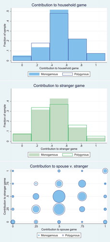
Figure 1 first shows histograms of contributions rates to the common pot in the spouse and stranger games, by marriage type. The histograms show roughly similar distributions, with monogamous spouses slightly more likely to contribute 2 tokens in the stranger and spouse games but less likely to contribute 1; the differences across distributions are not statistically significant (spouse games: Pearson ${\chi }^2=4.25,$ p-value = 0.373; stranger games: Pearson ${\chi }^2=4.45,$ p-value = 0.349). Figure 1 also shows a scatter plot of contributions to the spouse game by contributions to the stranger game, with the size of the circle or dot indicating the percentage of the sample making that choice. The plot shows that while many people contribute the same number of tokens to the spouse and stranger games (seen along the diagonal), many also contribute more in the spouse game than in the stranger game. These patterns do not differ by marriage type.¹³

Figure 1. Contribution summary statistics

Note: The figures show histograms of contributions to the common pot in the spouse and stranger games, as well as a scatter plot of behaviour in each with sizes of the dots indicating the number of respondents in each bin.

Table 4 shows summary statistics of contributions to the common pot for the stranger and spouse games by gender and marriage type. The first three rows show similar statistics to those shown in Table 2: means, standard deviations, and sample sizes are shown for monogamous husbands, monogamous wives, polygynous husbands, polygynous first wives, and polygynous second and third wives; followed by differences between monogamous and polygynous husbands, monogamous and polygynous first wives, and polygynous first and second and third wives along with standard errors. The fourth row shows differences between contributions to the stranger and first spouse game for each group, along with standard errors. The fifth row shows, for polygynous individuals who played two spouse games, differences between the first and second spouse games along with standard errors. The final two lines of the table show the fraction of respondents who said the games were ‘easy to understand’ or ‘very difficult to understand,’ with ‘a bit difficult to understand’ omitted.

Table 3. Asset summary statistics

	Mono	Mono	Poly	Poly	Poly	Husband	First Wife	Poly Wives
	Husbands	Wives	Husbands	First Wives	Second+ Wives	differences	difference	differences
	mean(sd)[N]	mean(sd)[N]	mean(sd)[N]	mean(sd)[N]	mean(sd)[N]	b(se)	b(se)	b(se)
Number cows for bride wealth		5.83		6.23	5.07		0.40	−1.16
		(2.98)		(2.87)	(1.84)		(0.34)	(0.31)***
		[172.00]		[134.00]	[117.00]
Zero cows for bride wealth		0.06		0.01	0.02		−0.04	0.00
		(0.23)		(0.12)	(0.13)		(0.02)*	(0.02)
		[179.00]		[138.00]	[121.00]
Don’t know how many cows for bride wealth		0.03		0.02	0.03		−0.01	0.00
		(0.18)		(0.15)	(0.16)		(0.02)	(0.02)
		[178.00]		[137.00]	[120.00]
Cash for bride price		26,643.84		20,601.69	45,312.55		−6,042.14	24,710.86
		(42,807.14)		(38,175.51)	(76,591.20)		(5,051.10)	(8,053.21)***
		[146.00]		[118.00]	[96.00]
Zero cash for bride price		0.47		0.57	0.41		0.09	−0.15
		(0.50)		(0.50)	(0.49)		(0.06)	(0.06)**
		[179.00]		[138.00]	[121.00]
Don’t know how much cash for bride price		0.18		0.14	0.20		−0.04	0.06
		(0.39)		(0.35)	(0.40)		(0.04)	(0.05)
		[178.00]		[137.00]	[120.00]
Savings	41,996.29	4,811.53	119,836.36	4,302.21	5,342.02	77,840.08	−509.32	1,039.81
	(165,437.37)	(27,673.30)	(501,514.65)	(18,854.57)	(37,122.43)	(40,036.06)*	(2,762.32)	(3,621.60)
	[175.00]	[178.00]	[165.00]	[136.00]	[119.00]
Zero Savings	0.77	0.75	0.72	0.81	0.82	−0.05	0.06	0.01
	(0.42)	(0.44)	(0.45)	(0.39)	(0.38)	(0.05)	(0.05)	(0.05)
	[175.00]	[178.00]	[165.00]	[136.00]	[119.00]
I own land	0.51	0.14	0.59	0.23	0.17	0.08	0.09	−0.05
	(0.50)	(0.35)	(0.49)	(0.42)	(0.38)	(0.05)	(0.04)**	(0.05)
	[179.00]	[179.00]	[169.00]	[137.00]	[120.00]
I keep all land if divorce	0.88	0.32	0.91	0.42	0.48	0.03	0.10	0.06
	(0.33)	(0.48)	(0.29)	(0.50)	(0.51)	(0.04)	(0.13)	(0.14)
	[92.00]	[25.00]	[99.00]	[31.00]	[21.00]
I own cows	0.97	0.95	0.92	0.99	0.98	−0.04	0.04	−0.01
	(0.18)	(0.22)	(0.27)	(0.09)	(0.13)	(0.02)*	(0.02)**	(0.01)
	[177.00]	[179.00]	[168.00]	[137.00]	[120.00]
I keep all cows if divorce	0.51	0.51	0.52	0.49	0.57	0.01	−0.02	0.08
	(0.50)	(0.50)	(0.50)	(0.50)	(0.50)	(0.06)	(0.06)	(0.06)
	[170.00]	[169.00]	[155.00]	[136.00]	[118.00]

Notes: Summary statistics for those included in the main analysis are shown in columns 1–5, split by player gender and marriage type. Means are shown in straight text, standard deviations in parentheses, and sample size in brackets. Column 6 shows the difference between monogamous and polygynous husbands, with standard errors of a t-test for difference in means in parentheses. Column 7 shows the difference between monogamous wives and polygynous first wives. Column 8 shows the difference between polygynous first wives and polygynous second and third wives. *p < 0.1; **p < 0.05; ***p < 0.01

Table 4. Game summary statistics

	Mono	Mono	Poly	Poly	Poly	Husband	First Wife	Poly Wives
	Husbands	Wives	Husbands	First Wives	Second+ Wives	differences	difference	differences
	mean(sd)[N]	mean(sd)[N]	mean(sd)[N]	mean(sd)[N]	mean(sd)[N]	b(se)	b(se)	b(se)
Contribution to Stranger	0.44	0.43	0.48	0.42	0.43	0.04	−0.01	0.01
	(0.21)	(0.25)	(0.23)	(0.25)	(0.26)	(0.02)*	(0.03)	(0.03)
	[180.00]	[180.00]	[170.00]	[142.00]	[128.00]
Contribution to First Spouse	0.56	0.50	0.59	0.50	0.56	0.03	−0.00	0.06
	(0.22)	(0.23)	(0.22)	(0.24)	(0.25)	(0.03)	(0.03)	(0.03)*
	[180.00]	[180.00]	[127.00]	[127.00]	[109.00]
Contribution to Second Spouse			0.55	0.46	0.47			0.00
			(0.19)	(0.24)	(0.23)			(0.04)
			[109.00]	[75.00]	[75.00]
Stranger v. 1st spouse differences b(se)	−0.12	−0.07	−0.11	−0.07	−0.13
	(0.02)***	(0.02)***	(0.02)***	(0.02)***	(0.03)***
1st spouse v. 2nd spouse differences b(se)			0.04	0.03	0.09
			(0.03)	(0.04)	(0.04)**
Easy to understand	0.37	0.31	0.34	0.33	0.38	−0.03	0.02	0.05
	(0.48)	(0.46)	(0.48)	(0.47)	(0.49)	(0.06)	(0.05)	(0.06)
	[180.00]	[180.00]	[127.00]	[127.00]	[109.00]
Difficult to understand	0.33	0.32	0.28	0.27	0.23	−0.05	−0.05	−0.04
	(0.47)	(0.47)	(0.45)	(0.44)	(0.42)	(0.05)	(0.05)	(0.06)
	[180.00]	[180.00]	[127.00]	[127.00]	[109.00]

Notes: Summary statistics for those included in the main analysis are shown in columns 1–5, split by player gender and marriage type. Means are shown in straight text, standard deviations in parentheses, and sample size in brackets. Column 6 shows the difference between monogamous and polygynous husbands, with standard errors of a t-test for difference in means in parentheses. Column 7 shows the difference between monogamous wives and polygynous first wives. Column 8 shows the difference between polygynous first wives and polygynous second and third wives. Rows 1–3 show contributions to the stranger, first, and second spouse games. Row 4 shows the difference in contributions to the stranger and first spouse games, with standard error in parentheses. Row 5 shows the difference in contribution to the first and second spouse games. The last two lines show respondents’ reports of how easy the games were to understand. ‘A bit difficult’ is the omitted category. *p < 0.1; **p < 0.05; ***p < 0.01

In unconditional means, there are no significant differences in average contribution to the common pot in the stranger game across groups (42-48%), and the absolute differences across groups are small: wives contribute at similar rates while there is a small, marginally significant difference in contribution rates across monogamous and polygynous husbands.

Spouses contribute 46–59 per cent of their endowment to the common pot in the spouse games. This is productively inefficient; respondents forego an average of 189.2 XOF of household income, or 16 per cent of potential earnings, in order to maintain control over some of a smaller total amount of money. It is common to find that spouses do not maximise household income in lab-in-the-field games; see Munro (2017) for a review of the literature. Monogamous husbands contribute to their spouse game at similar rates to polygynous husbands in their first wife spouse game (56 v. 59%). Monogamous wives contribute at similar rates to their husbands as do polygynous first wives (50%). Polygynous second and third wives contribute marginally significantly more to their husbands than first wives (56 v. 50%). Polygynous husbands give less, but not significantly, to their second and third wives than to their first wives (55 v. 59%). Co-wives give less to each other (46 and 47%) than to their husband (50 and 56%), and the difference is significant for second and third wives (row 5). All groups give substantially more in their first spouse game than in the stranger game (row 4).¹⁴

In sum, Table 4 shows the first evidence that monogamous husbands and wives are no more or less efficient than are polygynous husbands and first wives in unconditional mean contributions. Second and third wives give more to their husband than do first wives, and give more to their husband than to their co-wife.

Unfortunately, our ability to study whether polygynous spouses treat each game symmetrically is limited because many polygynous families did not send the husband, senior wife, and a junior wife. The main analysis sample examines 170 polygynous husbands and one or more of their wives; only 60 polygynous households sent their husbands and two of their wives. Although polygynous households who sent all potential wives are likely different from those who did not, it is still interesting to examine general trends within this subsample. Section 8 of supplementary material provides descriptive statistics on this restricted sample. Patterns of contributions to the common pot are similar across the full sample and the restricted sample. In terms of treating each game symmetrically, most polygynous spouses in the restricted sample contribute equally to each spouse game (68% of husbands, 52% of senior wives, 53% of junior wives). When not contributing evenly, spouses usually contribute more to their first spouse than their second (23% of husbands, 32% of senior wives, 30% of junior wives), while husbands occasionally contribute more to the junior wife game than the senior (8%), senior wives sometimes contribute more to the co-wife than the husband (17%), and junior wives sometimes more to the co-wife than to the husband (17%).

4. Results

Table 5 shows differences in contributions to the common pot across polygynous and monogmous households conditional on demographic and household controls and enumerator fixed effects, with standard errors clustered at the household level. Columns 1 and 4 control for only enumerator fixed effects. Columns 2 and 5 add control variables for individual age, illiteracy status, and number of children, as well as household size, indices for asset and livestock wealth, and the number of lactating cows owned by the household. Columns 3 and 6 add controls for whether the individual is divorced, the age gap between the respondent and their playing partner, and whether the respondent found the games ‘very difficult’ to understand. The first three columns in Table 5 show OLS regressions of the contribution rate to the common pot in the spouse game on an indicator that the household is polygynous, while the last three columns add an indicator that the respondent is male interacted with the polygynous indicator.

Table 5. Regression analysis of contributions to the spouse game by gender and marriage type

	(1)	(2)	(3)	(4)	(5)	(6)
VARIABLES	Limited Controls	Basic Controls	Extended Controls	Limited Controls	Basic Controls	Extended Controls
Polygynous	−0.01	−0.02	−0.02	−0.00	−0.02	−0.02
	(0.02)	(0.02)	(0.02)	(0.02)	(0.02)	(0.02)
Male				0.06**	0.06**	0.08***
				(0.03)	(0.03)	(0.03)
Male x Polygynous				0.01	0.01	0.01
				(0.03)	(0.03)	(0.03)
Constant	0.56***	0.46***	0.46***	0.53***	0.45***	0.43***
	(0.04)	(0.05)	(0.05)	(0.04)	(0.05)	(0.06)
Observations	982	982	982	982	982	982
R-squared	0.03	0.05	0.05	0.05	0.06	0.07

Notes: The table shows OLS regressions of contribution to the spouse game by gender and marriage type. Columns 1 and 4 control for only enumerator fixed effects. Columns 2 and 5 add controls for individual age, illiteracy status, and number of children, as well as household size, indices for asset and livestock wealth, and the number of lactating cows owned by the household. Columns 3 and 6 add controls for whether the individual is divorced, the age gap between the respondent and their playing partner, and whether the respondent found the games ‘very difficult’ to understand. Standard errors are clustered at the household level. *p < 0.1; **p < 0.05; ***p < 0.01

Results show that there are no differences in giving across monogamous and polygynous households. Men give more on average in their spouse games than do women,¹⁵ but polygynous men give no more on average than monogamous men.

While Table 5 shows that there are no differences across monogamous and polygynous contribution rates overall, there are difference by playing pair in polygynous households. Table 6 shows regression results by dyad, while Figure 2 presents the results graphically.¹⁶ Polygynous husbands contribute more to their first wives (51%) than to their second and third wives (46%). Second and third wives contribute more to their husbands (48%) than to their co-wives (39%) and they contribute more to their husbands (48%) than first wives contribute to their husbands (42%). Monogamous husbands and polygynous husbands contribute more to their first wives (50% and 51%) than those wives do to their husbands (44% and 42%).

Table 6. Regression analysis of contributions to spouse game by dyad

	(1)	(2)	(3)
VARIABLES	Limited Controls	Basic Controls	Extended Controls
Mono husband to wife	−0.03	−0.01	−0.01
	(0.03)	(0.03)	(0.03)
Mono wife to husband	−0.09***	−0.07**	−0.07*
	(0.03)	(0.03)	(0.04)
1st wife to poly husband	−0.09***	−0.09***	−0.09**
	(0.03)	(0.03)	(0.04)
2nd+ wife to poly husband	−0.03	−0.03	−0.03
	(0.03)	(0.04)	(0.05)
Poly husband to 2nd+ wife	−0.05**	−0.05**	−0.05*
	(0.02)	(0.02)	(0.03)
1st wife to 2nd+ wife	−0.13***	−0.13***	−0.12***
	(0.03)	(0.03)	(0.03)
2nd+ wife to 1st wife	−0.12***	−0.12***	−0.12***
	(0.03)	(0.04)	(0.04)
Constant	0.62***	0.51***	0.51***
	(0.04)	(0.06)	(0.06)
Observations	982	982	982
R-squared	0.06	0.07	0.07
p-values of Wald tests between coefficients	– – – – – -	– – – – – -	– – – – – -
Mono H to Mono W = Mono W to Mono H	0.0260	0.0400	0.111
Poly H to 2nd W = 2nd W to Poly H	0.669	0.592	0.809
1st W to 2nd W = 2nd W to 1st W	0.919	0.850	0.976
Mono W to Mono H = 1st W to Poly H	0.925	0.510	0.502
Mono W to Mono H = 2nd W to Poly H	0.0730	0.225	0.343
1st W to Poly H = 1st W to 2nd W	0.192	0.196	0.299
2nd W to Poly H = 2nd W to 1st W	0.00500	0.00600	0.00900
1st W to Poly H = 2nd W to Poly H	0.0870	0.0880	0.142

Notes: The table shows an OLS regression of contribution to the spouse game by dyad. The omitted variable is monogamous wife giving to husband. Tests for equality between coefficients are shown beneath the regression table. Column 1 controls for only enumerator fixed effects. Column 2 adds controls for individual age, illiteracy status, and number of children, as well as household size, indices for asset and livestock wealth, and the number of lactating cows owned by the household. Column 3 adds controls for whether the individual is divorced, the age gap between the respondent and their playing partner, and whether the respondent found the games ‘very difficult’ to understand. Standard errors are clustered at the household level. *p < 0.1; **p < 0.05; ***p < 0.01

Figure 2. Contribution by dyad

Note: The figure shows coefficient estimates of contributions by dyad (regression results shown in column 3 of Table 1).

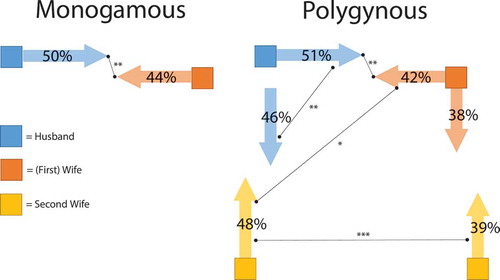
These tables and figures together show that differences between monogamous and polygynous households are overall small and not statistically different from zero. However, there are important differences by dyad within polygynous households. Polygynous husbands contribute less to their second and third wives than they contribute to their first wives; second and third wives give more to their husbands than first wives do. Co-wives also give less to each other than to their husbands, suggesting competition rather than collaboration among co-wives. Overall, this leaves second and third wives worse off than first wives.

5. Conclusion

In a series of lab-in-the-field games, we find that monogamous and polygynous households are equally productively inefficient on average. Members of both types of households are willing to forgo substantial household income in order to maintain individual control over resources. Consistent with our finding, a related paper finds that there are no differences across monogamous and polygynous households in terms of milk production or the gender gap in milk production (Hoel et al., 2020). However, average contributions at the household level mask differences in giving across dyads in polygynous households. Within polygynous households, we find that junior wives give more to their husbands than do senior wives, but receive less from their husbands than do senior wives. Co-wives also give less to each other than to their husbands, suggesting competition rather than collaboration among co-wives. Overall, junior wives receive fewer household resources compared to other members of the family.

Our results that junior wives are the worst off are consistent with other literature that shows that junior wives are more likely to suffer from domestic violence than senior wives (Hidrobo et al., 2018) and the children of junior wives are less healthy (Gibson & Mace, 2007; Matz, 2016). These results are also internally consistent with the descriptive statistics shown in Tables 2 and 3. In particular, junior wives receive fewer cattle compared to senior wives at the time of marriage and they are more likely to have been previously divorced. Divorce may well be the reason junior wives have less decision-making power, and in fact, contributions of husbands and first wives to second wives are smaller if they have been previously divorced (results available upon request).

Our results offer an interesting comparison to those in Barr et al. (2019) and Munro et al. (2019). All three studies find that both monogamous and polygynous families behave inefficiently and do not maximise household income. However, like Munro et al. (2019) and unlike Barr et al. (2019) we find that polygynous households are no more or less efficient overall than monogamous households. Unlike Barr et al. (2019) we find that polygynous husbands contribute less to their junior wives than to their senior wives, while junior wives give more to their husbands than do senior wives. Like Barr et al. (2019) we find that co-wives contribute less to each other than they do to their husbands. However, in our setting, the higher giving of second wives to husbands compensates for lower giving between co-wives, thus we do not see any differences on average between monogamous and polygynous relationships.

It is beyond the scope of this paper to disentangle what is driving these differences across studies; we believe economic activity, social norms, and cultural factors intersect with household structure in shaping contribution behaviour. All three papers study populations with distinct ethnicities that have different social norms and our paper, compared to Barr and Munro, has a distinct economic activity. In our setting, cattle is the main asset which is used for accumulating wealth, milk production, and meat production. While women generally tend to milk lactating cows in the morning and evening, men tend to ensure the cattle are fed and have water, which entails migrating with the cows daily and seasonally. In this context, the economic argument for polygyny laid out by Boserup (1970) that adding more wives increases production may not be as relevant. Adding more wives to increase production may also not be as relevant for the Munro et al. (2019) context where female seclusion inhibits women from working on the farms. Social norms around marriage and divorce are also distinct in our setting where marriages involve a transfer of both bride wealth (a gift of cows from the new husband’s family to the new wife herself) and bride price (a gift of cash from the new husband’s family to the new wife’s family) (Platteau & Gaspart, 2007). While in a divorce women may keep some of her bride wealth, if a women initiates the divorce, she must pay some of it back. Usually divorced women command a smaller bride price if they have lost their virginity.

There are several limitations to our study. First, it is possible that that monogamous families in our setting are simply ‘pre-polygynous’ and will add more wives in the future. The demographics in our sample support the idea that some monogamous marriages might become polygynous. Rossi (2019) notes that second marriages in Senegal usually take place 12 years after the first but the variation in the timing of the second marriage is large. In our sample the average polygynous husband is 8 years older than the average monogamous husband. Monogamous and polygynous individuals also display similarities in their altruism to strangers, risk preferences, time preferences, and other preferences associated with decision-making (see Tables B.1 and B.2 in Supplementary Materials). It is entirely possible that in this community for husbands and first wives, monogamy should not be thought of as an immutable trait but rather a temporary status. Boltz and Chort (2016) provides evidence that a risk of becoming polygynous changes behaviour even inside a monogamous marriage. While we do not find evidence to support the idea that adding a second wife to a household changes resource-sharing behaviour between the husband and first wife, it is possible that patterns are different overall in this group because everyone expects to become polygynous. Second, our small sample limits our ability to fully understand the mechanisms underpinning the contribution behaviour we observe. While we believe that the divorce status of junior wives is likely one reason for which husbands and senior wives contribute less to them, we cannot rigorously test this hypothesis or discard other related hypotheses. Relatedly, because not all individuals in polygamous relationships played the games, the junior and senior wives we observe are a selected sample and thus we cannot rigorously compare characteristics of senior wives to junior wives. While we conduct robustness checks (see supplementary material section 8) on polygynous households where husband and both senior and junior wives participated in the games, this sample is too small to further investigate any characteristics underpinning the contribution behaviour we observe.

Despite these limitations, our study has important policy implications. First we find that households are not efficient, implying non-cooperative household models such as separate spheres models are more appropriate in this setting (Lundberg & Pollak, 1993). In these models distribution within the household depends on an individual’s control over resources, implying that targeting public transfers to an individual matters for specific outcomes. Second, we find that while there is no evidence that polygynous households are more or less efficient than monogamous ones, junior wives in polygynous relationships are worst off in terms of how much they receive from husband net of how much they give to husband. This suggests that they do not have much influence over resource allocation decisions, and policy makers should be especially attentive to including their needs and perspectives. Policy makers have been concerned that poverty reduction plans need to be designed differently for polygynous households than monogamous families. Our results suggest that polygynous husbands and their first wives interact similarly to monogamous families, but that special attention is needed for junior wives.

Supplemental material

Supplementary Materials are available for this article which can be accessed via the online version of this journal available at https://doi.org/10.1080/00220388.2020.1762863

Disclosure statement

No potential conflict of interest was reported by the author(s).

Additional information

Funding

This work was supported by the European Union through the Consortium of International Agricultural Research Centers (CGIAR) Research Programs on Policies, Institutions and Markets (PIM); and Agriculture for Nutrition and Health (A4NH); the International Food Policy Research Institute (IFPRI)’s Strategic Innovation Fund; Colorado College’s Chapman and Soucheck Research Funds, Dean’s Fund, and Social Science Executive Committee to JBH; and the Eugene Rosenfeld Dissertation Award from the Pardee Research and Development (RAND) Graduate School to KW.

Notes

1. Polygamy refers to the institution of marriage with multiple members, either a single wife with more than one husband, polyandry, or a single husband with more than one wife, polygyny. In practice, nearly all polygamy is polygyny, and we will use the term polygyny for the sake of clarity.

2. Becker (1974) theory formalises the division of labour into his model of marriage markets, and the demand for wives specifically based on their productivity is tested in Jacoby (1995), who finds that men do have more wives when women are more productive. These studies are precursors to the cooperation mechanism in the model of Akresh et al. (2016).

3. Munro et al. (2019) was first published as the working paper Munro, Kebede, Tarazone-Gomez, and Verschoor (2010), and was a precedent to both Barr et al. (2019) and this study.

4. Because polygynous families form over time, we wanted to get an estimate of more completed family formations. Thus we look at marital status for the oldest women in the DHS, then assuming that those families would not add more wives later in life.

5. It is not possible to change the legal type of marriage at a later date.

6. The size of the gender gaps is not different in monogamous and polygynous households.

7. In November 2014, the exchange rate was 524 XOF per USD.

8. In a related paper, Hoel2019 show that households that behave more efficiently in the lab report less collaborative decision-making in milk production.

9. Hoel (2015) found that most spouses made the same allocation in a public dictator game as they did in a secret dictator game in Kenya.

10. Respondents were not allowed to participate until they could answer the test questions correctly. After playing the games, respondents were asked if in general they found the activities very difficult, a bit difficult, or easy to understand. They were also asked if they found it very difficult, a bit difficult, or easy to choose what to do. 31 per cent of respondents said it was very difficult to understand, while 26 per cent said it was very difficult to choose what to do. Table 4 shows that there are no differences in understanding across monogamous and polygynous husbands and wives. Contributions in the spouse games are not significantly related to self-reported understanding or difficultly choosing, after controlling for demographics and enumerator fixed effects. Results are robust to excluding respondents who said the games were very difficult to understand (available on request).

11. If there was more than one such pair in the household, preference was given to married household members who were responsible for delivering milk to LDB. If there was more than one such pair delivering milk to LDB, invited participants were selected at random. If the husband had more than two wives, two were selected at random to be invited. Results are robust to excluding 3+ wife families, available on request.

12. There are 111 second wives and 17 third wives in the sample.

13. See Supplementary material section 9 for more on robustness of game design.

14. In addition to differences in average contribution rates, we can also look at the mean linear difference between contribution in the household games and stranger game. 84 per cent of respondents give the same or more in their spouse game than they do in their stranger game. This further suggests that play in the games was not random.

15. This is also a common finding in the spouse games literature; see Munro (2017) for a summary of the literature.

16. Note that the omitted category in this regression is polygynous husband contribution to the first wife, so several relevant comparisons are not shown directly in the table. Tests of equality between coefficients are shown in the panel beneath the main regression table.

References

- Akresh, R., Chen, J. J., & Moore, C. T. (2016). Altruism, cooperation, and efficiency: Agricultural production in polygynous households. Economic Development and Cultural Change, 64(4), 661–696.
- Amey, F. K. (2002). Polygyny and child survival in West Africa. Social Biology, 49(1–2), 74–89.
- ANSD and ICF. (2018). Sénégal: Enquête démographique et de santé continue (EDS-Continue 2017). Technical report. Rockville, MD.
- Antoine, P., et al. (2002). Les complexités de la nuptialité: de la précocité des union féminines à la polygamie masculine en Afrique. In G. Caselli, J. Vallin, & G. Wunsch (Eds.), Démographie: analyse et synthèses (volume II: Les déterminants de la fecondité) (pp. 75–102). Paris: INED.
- Arthi, V., & Fenske, J. (2018). Polygamy and child mortality: Historical and modern evidence from Nigeria’s Igbo. Review of Economics of the Household, 16(1), 97–141.
- Barr, A., Dekker, M., Janssens, W., Kebede, B., & Kramer, B. (2019). Cooperation in polygynous households. American Economic Journal: Applied Economics, 11(2), 266–283.
- Becker, G. S. (1974). A theory of marriage: Part II. Journal of Political Economy, 82(2, Part 2), S11–S26.
- Becker, G. S. (1991). A treatise on the family. Cambridge, MA: Harvard University Press.
- Boltz, M., & Chort, I. (2016). The risk of polygamy and wives’ saving behavior. The World Bank Economic Review, 33(1), 209–230.
- Boserup, E. (1970). The role of women in economic development. New York: St. Martin’s.
- Bove, R., & Valeggia, C. (2009). Polygyny and women’s health in sub-Saharan Africa. Social Science & Medicine, 68(1), 21–29.
- Damon, A. L., & McCarthy, A. S. (2019). Partnerships and production: Agriculture and polygyny in Tanzanian households. Agricultural Economics, 50(5), 527–542.
- Gibson, M. A., & Mace, R. (2007). Polygyny, reproductive success and child health in rural Ethiopia: Why marry a married man? Journal of Biosocial Science, 39(2), 287–300.
- Hadley, C. (2005). Is polygyny a risk factor for poor growth performance among Tanzanian agropastoralists? American Journal of Physical Anthropology, 126(4), 471–480.
- Hampshire, K. R., & Smith, M. T. (2001). Consanguineous marriage among the Fulani. Human Biology, 73(4), 597–603.
- Hidrobo, M., Heath, R., & Roy, S. (2018). Cash transfers, polygamy, and intimate partner violence: Experimental evidence from Mali. IFPRI Discussion Paper (1785).
- Hoel, J. B. (2015). Heterogeneous households: A within-subject test of asymmetric information between spouses in Kenya. Journal of Economic Behavior & Organization, 118, 123–135.
- Hoel, J. B., Hidrobo, M., Bernard, T., & Ashour, M. (2020). What do intra-household experiments measure? Evidence from the lab and field. Mimeo.
- Jacoby, H. G. (1995). The economics of polygyny in sub-saharan africa: Female productivity and the demand for wives in Côte d’Ivoire. Journal of Political Economy, 103(5), 938–971.
- Jankowiak, W., Sudakov, M., & Wilreker, B. C. (2005). Co-wife conflict and co-operation. Ethnology, 44, 81–98.
- Kazianga, H., & Klonner, S. (2009). The intra-household economics of polygyny: Fertility and child mortality in rural Mali. Munich Personal RePEc Archive (12859).
- Lundberg, S., & Pollak, R. A. (1993). Separate spheres bargaining and the marriage market. Journal of Political Economy, 101(6), 988–1010.
- Matz, J. A. (2016). Productivity, rank, and returns in polygamy. Demography, 53(5), 1319–1350.
- Munro, A. (2017). Intra-household experiments: A survey. Journal of Economic Surveys, 32(1), 134–175.
- Munro, A., Kebede, B., Tarazona-Gomez, M., & Verschoor, A. (2019). The lion’s share. an experimental analysis of polygamy in northern Nigeria. Economic Development and Cultural Change, 67(4), 833–861.
- Munro, A., Kebede, B., Tarazone-Gomez, M., & Verschoor, A. (2010). The lion’s share: An experimental analysis of polygamy in northern Nigeria. GRIPS Discussion Papers 10.
- Parisse, M. (2012). Developing local dairy production: The Laiterie du Berger, Senegal. Field Actions Science Reports, 6, 1–6.
- Platteau, J.-P., & Gaspart, F. (2007). The perverse effects of high brideprices. World Development, 35(7), 1221–1236.
- Rossi, P. (2019). Strategic choices in polygamous households: Theory and evidence from Senegal. The Review of Economic Studies, 86(3), 1332–1370.
- Sellen, D. W. (1999). Polygyny and child growth in a traditional pastoral society. Human Nature, 10(4), 329–371.
- Shepard, L. D. (2013). The impact of polygamy on women’s mental health: A systematic review. Epidemiology and Psychiatric Sciences, 22(1), 47–62.
- Timaeus, I. M., & Reynar, A. (1998). Polygynists and their wives in sub-Saharan Africa: An analysis of five Demographic and Health Surveys. Population Studies, 52(2), 145–162.
- Wagner, N., & Rieger, M. (2015). Polygyny and child growth: Evidence from twenty-six African countries. Feminist Economics, 21(2), 105–130.