Poverty Trap or Means to Escape Poverty? Empirical Evidence on the Role of Environmental Income in Rural Nepal

Abstract

Understanding how poverty persists and how this affects environmental reliance has policy implications for poverty reduction and environmental conservation. Employing a panel data-set from rural Nepal, we shed light on this issue, using a combination of parametric and nonparametric models. Results show that, as a population, households will converge at a single equilibrium point in the long-term, hence indicating the absence of a poverty trap. The exact asset level of this single equilibrium point, which indicates the absence of a poverty trap, varies between groups of households (for example, based on location, marital status). Based on the convergence point of the entire study population, two groups of households are identified: one situated above the convergence point and another situated below the point. Total environmental income, that is, all income from forest and non-forest environments, is very important to households below the convergence point. Although total environmental income is not a major contributor to asset accumulation, its non-forest component is a significant and positive contributor. We attribute the importance to their looser restriction to access, than for forest resources. Hence, securing greater access to forests without affecting the conservation priorities will help improve the contribution of forest resources to poverty reduction.

1. Introduction

The contribution of environmental income to rural livelihoods in the Global South is increasingly being recognised (Angelsen et al., 2014; Byron & Arnold, 1999; Rasul, Karki, & Sah, 2008). Results from a global-comparative analysis of environmental income (that is, income generated form non-cultivated environmental resources) from 8000 households in 24 countries in the Global South recently showed that environmental income accounts for 28 per cent of total household income (Angelsen et al., 2014). There is a general consensus in academia about the importance of environmental resources in providing rural livelihoods with a source of food, fuel, fodder, medicine, and construction material which can be used for subsistence and income generation (Djoudi, Vergles, Blackie, Koffi Koame, & Gautier, 2015; Hogarth, Belcher, & Campbell, 2013; Jiao et al., 2019; Pouliot & Treue, 2013). Empirical evidence on the role of environmental resources for rural livelihoods have important welfare implications as they allow researchers and policy-makers to understand the impact of deforestation and environmental degradation on poor people’s lives, enabling effective design of development and conservation strategies (Angelsen et al., 2014; Angelsen & Wunder, 2003; Cavendish, 2002; Vedeld, Angelsen, Sjaastad, & Berg, 2004).

Following the UN’s Millenium Development Goals and Sustainable Development Goals, attention has been shifted to the possible link between poverty alleviation and environmental income (Scharlemann et al., 2016). In Nepal, forests and other non-cultivated environmental resources have become the focus of many development and poverty alleviation efforts (Nightingale, 2003), partly because they are considered critical for subsistence and income generation for rural households (Adhikari, Di Falco, & Lovett, 2004; Charlery & Walelign, 2015; Walelign, Charlery, Smith-Hall, Chhetri, & Larsen, 2016). While available research supports the idea that environmental resources can generate income which can contribute to poverty alleviation ‘for some people in some places’ (Roe, Elliott, Sandbrook, & Walpole, 2013), depending on specific contextual factors and product-specific characteristics (Shackleton, Shackleton, Buiten, & Bird, 2007), empirical evidence on the question is too limited to lead to firm conclusions. The underlying arguments linking environmental income and poverty alleviation include the role of non-cultivated environments in filling seasonal income gaps and as safety nets in times of emergency (Byron & Arnold, 1999; Fisher & Shively, 2005; McSweeney, 2004; Pattanayak & Sills, 2001; Shackleton et al., 2007; Yemiru, Roos, Campbell, & Bohlin, 2010). Other scholars, however, argue that inferior characteristics of environmental resources keep households trapped in poverty (Angelsen & Wunder, 2003; Barbier, 2010; Skoufias, 2003; Vira & Kontoleon, 2013; Wong & Godoy, 2003).

While understanding the contribution of environmental resources in breaking rural poverty traps in the Global South is crucial to ensure the formulation of appropriate pro-poor and sustainable environmental and development policies, household-level analyses linking environmental resource use and poverty transitions have been hampered by a lack of suitable quantitative datasets. Most empirical studies on environmental income in the Global South use one-year income data to categorise households into poverty groups (for example, Babulo et al., 2009; Reddy & Chakravarty, 1999; Walelign, 2013). Therefore, they provide a static analysis of the environment-poverty nexus. Panel data is needed for a dynamic, empirical investigation of the links between environmental income and household poverty movements. Using a two-wave panel data, Walelign et al. (2019) empirically investigated the role of environmental resources in asset accumulation for rural households in Nepal. However, the study has three limitations. First, the study emphasises asset accumulation and did not test the presence of poverty traps. Second, the study considered four type of assets (that is, implements, livestock, bank saving, and jewellery) and overlooked very important assets that are relevant in understanding poverty. These include social capital (for example, help from the community, trust on the community), and human capital (for example, education, experience). Third, the paper did not distinguish the effect of different sources of environmental income (forest vs non-forest and cash vs non-cash). These limitations hamper our understanding of the effect of environmental income in breaking poverty traps.

In this paper, we investigate the effect of environmental income on poverty traps. Using a unique three-wave environmentally-augmented income and asset panel dataset, we first apply the poverty trap theory of Carter and Barrett (2006) to test for the presence of poverty traps among the sample households. We included a wide variety of assets in testing for poverty traps. Then, we identify groups of households with different asset accumulation paths and assess the importance of environmental income to these groups. Lastly, we examine the covariates of asset dynamics, with specific focus on environmental income, allowing us to conclude on the environment-poverty nexus. In the models, we examined the differential effect of forest and non-forest environmental income on one hand, as well as cash and non-cash environmental income, on the other hand.

2. Methods

2.1. Poverty trap theory

Generally, if households with low asset values, often the poor, accumulate assets at a greater rate than households with high asset values, often the better-off, neoclassical assumption of diminishing returns to assets will hold and the asset poor households will eventually catch up with the asset rich households by moving to a single long-term equilibrium (Islam, 2003). If households with low asset values accumulate assets at a lower rate than households with high asset values or cannot accumulate assets, this induces a reinforcement of poverty and the poor households stay trapped in poverty (Barret, Garg, & McBride, 2016; Carter & Barrett, 2006). Different frameworks of poverty traps exist depending on the potential cause of poverty traps. These frameworks, among others, include: (i) nutrition-based poverty traps, where lack of enough calories is posited as the main cause of poverty traps (Banerjee & Duflo, 2011), (ii) health poverty traps, where poor health and the consequent medical costs to return to normal health and inability to work are posited as the cause for poverty traps (Banerjee & Duflo, 2011), and (iii) energy poverty traps, where reliable, efficient, and sufficient energy sources and the consequent inability to accomplish daily tasks more efficiently is posited as the main cause of poverty traps (Jones, 2016). All these studies explain poverty traps as households’ inability to escape poverty due to the mechanisms that inhibit their capacity for income generation and accumulation of assets.

To understand and illustrate the concept of poverty traps, in the current paper we use the asset dynamics framework developed by Carter and Barrett (2006) because assets are less seasonal, and stochastic, as well as less prone to measurement error than income and consumption measures. In this framework, assets are used as a measure of household welfare dynamics and encompass ‘conventionally privately held productive and financial wealth, as well as social, geographic and market access positions that confer economic advantage’ (Carter & Barrett, 2006, p. 179). Figure 1 (adapted from Adato, Carter, & May, 2006) illustrates the framework and the theory of poverty traps. In the figure, the x-axis displays initial asset index¹ while the y-axis displays current asset index. The 45-degree line represents a situation in which the current and the initial asset holdings are equal and hence any point on this line represents a dynamic equilibrium.

Figure 1. Hypothetical household asset dynamics (adapted from Adato et al., 2006)

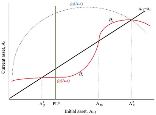
Households’ welfare dynamics depends on the marginal returns to initial assets and scale of returns to assets. Based on this, two asset dynamics paths and patterns of implied poverty traps can be identified. The first one is the case in which the entire asset distribution is concave downward, shown with the function, $g_1\left(A_{t-1}\right)$, where the marginal return on assets changes sign (from positive to negative) only once. This implies that households accumulate assets over time and whatever their initial asset holding, will eventually converge to a single stable dynamic asset equilibrium,² $A_c^{\ast }$, in the long-term (Adato et al., 2006). On the other hand, if the part of the asset distribution is ‘S-shaped’ (shown with the function $g_2\left(A_{t-1}\right)$), household asset accumulation path cuts the 45-degree line (represents the equality between current and initial assets) three times, resulting in two stable ($A_p^{\ast }$ and $A_c^{\ast }$) and one unstable ($A_m$) dynamic equilibrium points. At the unstable equilibrium, the asset dynamics bifurcate and this results in multiple equilibria (Adato et al., 2006; Zimmerman & Carter, 2003). A household above the unstable equilibrium accumulates assets over time and moves to the upper stable equilibrium, $A_c^{\ast }$, while a household below is too poor to accumulate assets over time and hence, moves to the lower equilibrium, $A_p^{\ast }$, in the long-term (Zimmerman & Carter, 2003) and becomes trapped there.

Testing for the presence of poverty traps can be done in both a relative and absolute sense. In terms of the relative sense, the number of equilibrium points determines the presence of poverty traps – meaning that a single equilibrium point implies no poverty trap while multiple equilibria imply the presence of a poverty trap, where the lowest equilibrium ($A_p^{\ast }$) is associated with that poverty trap (Carter & Barrett, 2006; Giesbert & Schindler, 2012). This is because the lowest equilibrium point is associated with low living standards equivalent to poverty, while the highest equilibrium point is associated with high living standards equivalent to non-poverty. Analysing poverty in terms of an absolute sense makes reference to a poverty line ($P{L}^{\ast }$) to test for the presence of poverty traps, meaning that regardless of the number of equilibrium points, any equilibrium point which falls below the poverty line is associated with a poverty trap (Naschold, 2012). To illustrate this, in Figure 1, a poverty trap exists for the asset accumulation path represented by $g_2\left(A_{t-1}\right)$ as one of its stable equilibrium points ($A_p^{\ast }$) falls below the poverty line. In this paper, we employ the relative approach to assessing the presence of a poverty trap in the study population, as our created asset index does not allow for the calculation of a poverty line, which is required for the absolute approach (see creation of asset index section below). Consequently, following Carter and Barrett (2006) and Giesbert and Schindler (2012), we consider that poverty traps exist in our study population if at least two stable and one unstable equilibrium points are present, and the lowest equilibrium is a poverty trap.

2.2. Data source and data collection

2.2.1. Study area

The study sites consist of four village development committees (VDCs) from three districts which span across the agro-ecological zones in Nepal (Meilby, Puri, Christensen, & Rayamajhi, 2006): Lete and Kunjo VDCs in Mustang district in the Himalayas, Hemja VDC in Kaski district in the mid-hills, and Chainpur VDC in Chitwan district in the Terai.³ Table 1 provides a breakdown and brief description of the sample districts and village development committees. Data collection was conducted by the Community Based Forest and Tree Management in the Himalaya (ComForM) project, under the Poverty Environment Network (PEN) study programme.

Table 1. Key descriptions of the study areas

District	VDC	# of households (2006)	Sampled households (2006)	Elevation (m.a.s.l.)	Market access
Chitwan	Chainpur	1542	207	350	Motorable, gravel road (all reason)
Kaski	Hemja	222	114	1000	Tarmac road, bus service
Mustang	Kunjo	163	88	2200–3000	2006: plane and foot 2009: motorable (dry-weather) gravel road
	Lete	174	98

The study sites in Chitwan and Kaski districts are similar in terms of accessibility and infrastructural development. They both have year-round motorable road access to market centres, and villagers are readily able to engage in skilled and unskilled employment opportunities in the connected town centres. However, the study sites in Mustang are more remote, with less infrastructural development. The recent construction of a tertiary (dry-weather) road, connecting the town centres of Beni and Jamsom, (transecting Lete VDC) has significantly increased access to Lete and Kunjo during the dry seasons. Though the VDCs of Mustang are becoming more connected to town centres and other districts than before, due to the construction of the road, they remain more reliant on traditional livelihood strategies and experience higher poverty indices than the VDCs in the other districts (poverty rates of 42.3% in the Mountains, 24.3% in the Mid-hills and 23.4% in the Tarai regions [CBS, 2013]).

Local restrictions are placed on the collection of products from public forests, including cash and subsistence products such as timber and firewood. Each sample village has at least one community forest/forest conservation area with forest management plan and constitution. Restrictions vary across these village level forest conservation entities and forest products according to their constitution and depending on the conditions of the forest. Membership is required to have access to the forests (all sample households are members of at least one community forest user group/forest conservation area) and all members are believed to have equal access to forest products. Access to environmental products is not restricted to the same degree on other public land and there is no restriction to owners of private land with trees (Larsen et al., 2014).

2.2.2. Data collection

Data was collected in 2006, 2009, and 2012. Data collection and handling followed the PEN guidelines⁴ to ensure consistency across sites. The PEN prototype questionnaire formed the backbone of the data collection instruments at the village and household levels. Household economic data was collected on a quarterly basis (four visits per year) to facilitate easy recall, improving the quality of the data. The quarterly datasets in each year were summed to result in annual economic data. Household assets and village level data was collected at the beginning and again at the end of each year. Income is defined as the value added of labour and capital, and environmental income is defined as income generated through the extraction of products from non-cultivated sources (for example, forests, grasslands, bushlands, wetlands, fallows and wild plants, and animals harvested from croplands) (Angelsen et al., 2014). This is the total value of cash or goods obtained from the trade of goods and/or services by members of the household, less the cost of all inputs except labour provided by household members. The cost of household labour is not factored into the income calculation due to difficulties in estimation and the poor labour markets in the study sites. All goods produced or collected by the household and used for home consumption (subsistence) are valued at market prices within the community and counted as part of household income (Centre for International Forestry research [CIFOR], 2007). In the absence of market prices due to fragile or thin markets, alternative valuation methods were used – including bartered prices, substitute goods, embedded time, distant market prices, and contingent valuation – as described in Wunder, Luckert, and Smith-Hall (2011). Therefore, income from the environment, crops, and livestock all have a cash and subsistence component. All nominal variables were put in real terms using the national consumer price index (CPI). All assets shared by household members in production and consumption (for example, value of implements, land holding) as well as all income values were divided by adult equivalent units (aeu) in the household, in order to allow inter-household comparisons.

The 2006 data was collected from 507 randomly selected households across the three districts in the four VDCs (Table 1). Of the 507 initially sampled households, 446 were resurveyed in 2009. From these 446 households, 428 were resurveyed in 2012. This results in an attrition rate of 12 per cent between 2006 and 2009, 4 per cent between 2009 and 2012, and 16 per cent over the six-year period. Analysis of the effect of attrition based on dynamic and static attrition tests using appropriate models (for example, probit) show that although attrition is non-random, its effect on the estimates from the data is benign for the current estimations (see Appendices D, E, and Walelign, 2016a). One household was dropped from further analysis due to implausibly high total income; thus, we made use of the balanced dataset covering 427 households over the three-year periods.

2.3. Creation of the composite asset index

Assets were measured in different units (Appendix A). Thus, we needed to construct a single asset variable to avoid interpretation difficulties as well as the ‘curse of dimensionality’ – estimation difficulties due to the number of asset variables measured in different units (Naschold, 2013). In the literature, this has been done in two ways: the livelihood weighted asset index (Adato et al., 2006) and data reduction statistical tools, particularly principal factor analysis (PFA) (Naschold, 2013) or principal component analysis (PCA) (Filmer & Pritchett, 2001). Neither method of asset index construction is superior to the other and the choice depends on the purpose of the study or on the basis of data availability (Naschold, 2013). In this paper, the PFA approach is selected over PCA because we are interested in explaining the common variance among assets and dealing with measurement errors. The PFA approach is also preferred over the livelihood-weighted approach (for example, Adato et al., 2006) as we would like to examine the pattern of environmental income for the different asset dynamics groups. This would not be possible if we employed the livelihood weighted approach because environmental income would be part of the livelihood weighted asset index. Additionally, the Kaiser-Meyer-Olkin measure of sampling adequacy test (see SM1 in Supplementary Materials) and Bartlett’s test of sphericity (with${\mathrm{X}}^2(105)=210.12;\mathrm{P}-\mathrm{v}\mathrm{a}\mathrm{l}\mathrm{u}\mathrm{e}<0.01$) suggest PFA is appropriate for our data.

According to the Kaiser criterion, two principal component factors should be kept for further analysis. However, both factor scores tend to provide similar information towards households’ asset possession and dynamics (see SM 2, SM 3, SM3 4 in Supplementary Materials and Figure 2). On this basis and as the first factor contains the largest share of the common variance relative to other factors (including the second), we used the first principal factor score in the subsequent analysis. The factor represents an asset score, a unit-less composite indicator for asset possession and is interpreted in relative (comparative), not in absolute, value, implying that higher values indicate a larger asset possession.

Following Naschold (2013) and Barrett et al. (2006), to allow for comparison of asset indices across time, we use the pooled asset data to create the asset index. In order to account for differences that affect factor weights over time, we include year dummies in the factor analysis. Following Naschold (2013, 2012) and Giesbert and Schindler (2012), we included both productive and non-productive assets in the PFA analysis. This is because both asset categories play important functions to the livelihood of households: productive assets are mainly used in production while non-productive assets have other functions, including for example, having access to a source of information (for example, TV). Non-productive assets can often be converted to productive assets if need for productive assets arises.

2.4. Modelling poverty traps

After generating the asset index, we model the asset dynamics of households to test for the presence of poverty traps using nonparametric and semiparametric regression models.⁵ The nonparametric model can be specified as:

(1) $A_{i,t}=f\left(A_{i,t-1}\right)+{\epsilon }_{i,t}$(1)

Where $A_{i,t}$ is the asset index at time $t$, $A_{i,t-1}$ is lagged asset index and ${\epsilon }_{i,t}$ is an error term which has normal distribution with zero mean and constant variance. Different techniques of estimating Equation (1)(1) $A_{i,t}=f\left(A_{i,t-1}\right)+{\epsilon }_{i,t}$(1) (for example, locally weighted scatterplot smoother, kernel-weighted local linear smoother) tend to lead to similar results (Naschold, 2013). Hence, in this paper, Equation (1)(1) $A_{i,t}=f\left(A_{i,t-1}\right)+{\epsilon }_{i,t}$(1) is estimated with local polynomial smoothing regression with Epanechnikov kernel weights. Though the nonparametric models are flexible as they do not assume any functional form, one major limitation of modelling asset dynamics through nonparametric regression is that it is not possible to account for covariates other than the lagged asset values.

To allow for the inclusion of other explanatory variables and identify the covariates of households’ asset accumulation, with a focus on households’ income from environmental resources, we rely on a parametric model. Following other previous empirical studies on asset growth (Giesbert & Schindler, 2012; Quisumbing & Baulch, 2013), the fourth-degree polynomial parametric regression model can be specified as:

(2) $A_{i,t}-A_{i,t-1}={\beta }_0+{\sum }_{j=1}^4{\beta }_j{A}_{i,t-1}^j+\delta X_{i,t-1}+{\epsilon }_{it}$(2)

Where $A_{i,t}$ is the asset index at time $t$, $A_{i,t-1}$ is lagged asset index, $x_{i,t-1}$ is vector of lagged explanatory variables (for example, household and household head characteristics, location dummies, income from environmental resources, and income from non-environmental sources), $\delta$ is the associated vector of coefficients, ${\sum }_{j=1}^4{A}_{i,t-1}^j$ is the fourth degree polynomial of lagged assets and ${\sum }_{j=1}^4{\beta }_j$ (that is, ${\beta }_1,{\beta }_2,{\beta }_3,and{\beta }_4$) is the associated vector of coefficients, ${\beta }_0$ is the regression intercept, and ${\epsilon }_{i,t}$ is an error term which has a normal distribution with zero mean and constant variance. A significant negative coefficient of $A_{i,t-1}$ (that is, ${\beta }_1$) suggests convergence in households’ asset dynamics meaning that asset poor households accumulate assets faster than their asset rich counterparts. A significant coefficient of ${\sum }_{j=2}^4{\beta }_j$ (that is, ${\beta }_2,{\beta }_3,and{\beta }_4$) suggests the presence of non-linearities in households’ asset accumulation. The choice of explanatory variables was advised by existing studies on rural livelihood and livelihood dynamics, rural poverty and poverty dynamics, and asset accumulation (for example, Abro, Alemu, & Hanjra, 2014; Adams, 1998; Barrett et al., 2006; Haddad & Ahmed, 2003; Giesbert & Schindler, 2012; Jiao, Pouliot, & Walelign, 2017; Krishna, 2007; May & Woolard, 2007; Winters et al., 2009). We also run alternative models disaggregating (i) total environmental income into forest and non-forest, (ii) total environmental income to cash and subsistence components, and (iii) total forest and non-forest environmental income into their cash and subsistence components. The disaggregation into forest and non-forest environmental income allows investigating the potentially different effects of the two sources of income on asset accumulation. The different effects can arise from the nature of institutions governing those resources and the products collected from forest and non-forest environments in Nepal: products collected from forest and non-forest environments differ in remuneration and access restriction. The disaggregation into cash and subsistence incomes accommodates the difference in the nature of these two types of income: while cash environmental income is converted into cash (through markets) and can either be used to fulfil household consumption necessities or can directly be invested in assets, subsistence environmental income is used by the households for direct consumption. Subsistence environmental income can also promote households’ investment in assets as it covers part of the households’ consumption needs, allowing part of the cash income (from other income sources) that would have been used for subsistence to be invested in asset accumulation. This means that cash and subsistence environmental income have direct and indirect effects on asset accumulation, respectively, and the sign and significance of the effects is context-specific.

We estimated Equation (2)(2) $A_{i,t}-A_{i,t-1}={\beta }_0+{\sum }_{j=1}^4{\beta }_j{A}_{i,t-1}^j+\delta X_{i,t-1}+{\epsilon }_{it}$(2) using the fixed effects panel data estimator for two major reasons. First, we suspect the presence of endogeneity arising from household time-invariant unobserved heterogeneity, and the fixed effects estimator is a powerful tool to wipe out the resulting bias. Second, the Hausman specification test (X²(13) = 869.46; P-value ˂ 0.01) rejects the null hypothesis that the random effects estimator is preferred over the fixed effects estimator.

One major issue which has been said to be linked to measuring poverty traps and dynamics is a potential bias arising from measurement errors and shocks/fluctuations in the welfare indicator resulting in extreme values in one or more periods and rendering the observation of the indicator without the measurement error or shocks/fluctuations to get close to the average of the indicator (the issue of regression towards the mean) (Bigsten & Shimeles, 2008; Dercon & Krishnan, 2000). However, the empirical models we employed here are not sensitive to these issues. This is because we use assets – rather than income and consumption expenditure – as a welfare measure, PFA to create the asset index which is robust to measurement errors, and the lagged asset index and shocks in the models. Hence, while the common bias due to measurement errors and shocks cannot be ruled out completely, these are not considered to have critically affected the results.

Given the short period (that is, six years) of our dataset and slow asset accumulation in rural communities of the Global South, following the literature (Giesbert & Schindler, 2012; Naschold, 2012, 2013), we assume all households follow the same asset accumulation path. Without this assumption, we would risk observing part of the long-term asset accumulation path of a household. However, we also relax this assumption to allow households in a specific socio-economic group to follow the same asset accumulation. This allows an observation of whether the convergence points differ by groups.

3. Results

3.1. Poverty traps

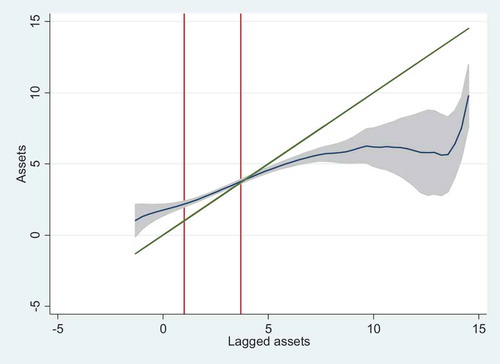
Figure 2 shows the estimated dynamic asset accumulation path (blue line), its 95 per cent confidence band (grey band), along with the 45-degree line (green line) which indicates the possible points of dynamic equilibrium for the entire pooled population (under the assumption of all households follow the same asset accumulation path) based on local polynomial nonparametric regression. The asset accumulation path, along with its upper and lower confidence bands, cross the 45-degree line (at the point of stable equilibrium) only once, suggesting the existence of a single dynamic equilibrium. Hence, no evidence for the presence of poverty traps in rural Nepal; rather, all households tend to move towards (converge at) a single equilibrium point in the long-term, although the equilibrium point tends to differ by socio-economic groups (see Table 2). This result was consistent across other estimation methods of asset dynamics and poverty traps that allow for the inclusion of explanatory variables, that is, fixed effects parametric model (Table 5) and penalised spline semiparametric regression (Appendix C). It was also consistent across two alternative measures of asset scores: total value of major types of natural, physical, and financial assets (that is, livestock, implements, saving, jewellery, and debt – as a measure of access to assets) and total land size (SM 5 and SM6 in Supplementary Materials). The approximate location of the stable equilibrium point for the entire pooled population is at 1.15 asset scores (Figure 2).

Figure 2. Household asset dynamics based on local polynomial regression.Note: Red vertical lines represent (from left to right) the lower bound of the confidence interval, the stable equilibrium point, and the upper bound of the confidence interval

Table 2. Equilibrium points by sub-groups of households estimated based on local polynomial nonparametric regression

	Approximate location of the equilibrium	95% confidence interval
		Lower bound	Upper bound
Sex of household head
Male	1.15	0.43	1.72
Female	1.15	−0.20	2.20
Head born in the village
Yes	1.1	0.50	1.71
No	0.85	0.10	1.45
Head married
Yes	1.13	0.52	1.70
No	1.85	−0.40	2.2
Location
Chitwan	1.52	1.05	2.05
Kaski	1.32	0.58	1.90
Mustang	0.10	−0.30	1.25
Shock
Yes	0.80	0.22	1.40
No	1.60	0.50	2.15

When we relax the assumption that all households, on average, follow a single asset accumulation path (as in the above analysis) and undertake population subgroup analyses, allowing all households in each subgroup to follow an asset accumulation path based on the characteristics of their subgroup, we find evidence for the presence of group specific equilibria (Table 2). Like the results for the pooled population, the subgroups each show the existence of a single dynamic equilibrium. Therefore, our findings do not suggest that all households in rural Nepal will converge at an identical convergence point or asset level. Rather, what is important is the presence of a single dynamic equilibrium for either the entire study population or for subgroups of that population, therefore pointing to the absence of a poverty trap. Households with a head born in the village had a higher equilibrium (1.1 asset scores) than households with a head born outside the village (0.85 asset scores). Households with an unmarried head move to different equilibria than households with a married head (1.85 and 1.13 asset scores, respectively). With regards to location, households living in Chitwan and Kaski were more likely to converge to a higher equilibrium (1.52 and 1.32 asset scores, respectively) while households living in Mustang are more likely to converge to a very low equilibrium (0.10 asset scores). Households who experienced negative shocks (in the form of moderate and severe shock) moved to a lower equilibrium (0.80 asset scores) than households who did not experience any shock (1.60 asset scores). However, male and female headed households appeared to move to the same equilibrium (1.15 asset scores). It is common that households may change their socio-economic status (for example, marital status of a household head), in which case the household follows the asset accumulation path of the new group and converge to the associated equilibrium point.

3.2. Household income sources and asset holdings

The distribution of households on the dynamic asset accumulation path (based on the local polynomial nonparametric regression) resulted in a great majority (n = 1193) of households below the stable equilibrium and very few above (n = 88). Dividing the population into these two groups – below and above the stable equilibrium – allowed an analysis of the differences in livelihoods and characteristics of households on different points of the dynamic asset accumulation path. Table 3 reports the mean and relative income (total and from each source) for households above and below the equilibrium. The total income of households above the stable equilibrium was about three times larger than the total income of households below the stable equilibrium. Income from remittances was the most important source for the households below the stable equilibrium while business was the most important income source for those above the stable equilibrium. Environmental income was the second and sixth most important income source for the households below and above the stable equilibrium, respectively. On average, households below the stable equilibrium generated more income from the environment than those above the stable equilibrium, but the difference was not statistically significant. Overall, the three most important income sources for the population, in order of importance, were business income, remittances, and environmental income.

Table 3. Mean income (from individual sources; in Nepalese Rupees, NRs) for the two different asset dynamics groups(identified based on local polynomial nonparametric regression)

	Below the equilibrium (n = 1193)		Above the equilibrium (n = 88)		Significance difference tests		Overall
Income sources	Abs.	Rel.	Abs.	Rel.	Abs. (F-statistic)	Rel. (Z-statistic)	Abs.	Rel.
Environmental income	7,356 (23,082)	16.92	6,034 (10,137)	4.32	0.28	3.11***	7,266 (22,433)	14.50
Crop income	4,97 (11,211)	11.45	7,521 (11,083)	5.38	4.23**	1.75**	5,151 (11,217)	10.28
Livestock income	6,198 (16,748)	14.25	14,858 (46,397)	10.63	15.07***	0.94	6,793 (20,306)	13.56
Remittances	8,619 (23,798)	19.82	5,561 (16,548)	3.98	1.40	3.68***	8,409 (23,380)	16.79
Support income	3,508 (7,752)	8.07	11,065 (18,790)	7.92	58.48***	0.05	4,028 (9,145)	8.04
Other income	4,782 (28,990)	11.00	23,572 (100,288)	16.86	19.72***	−1.67**	6,073 (38,586)	12.12
Business income	7,058 (57,528)	16.23	71,070 (402,193)	50.84	23.84***	−8.05***	11,456 (119,745)	22.87
Wage income	981 (2,450)	2.26	99 (361)	0.07	11.38***	1.38*	921 (2,377)	1.84
Total income	43,480 (77,945)	-	139,781 (425,472)	-	42.28***	-	50,096 (136,219)	-

Notes: Values in parenthesis are standard deviations of the mean; estimation based on the pooled data from the three periods. ***Significant at 1 per cent, **Significant at 5 per cent, *Significant at 10 per cent; Abs. = absolute, Rel. = relative. We used ANOVA significance test for the absolute incomes and z-test for proportions for relative incomes; the figures are adjusted for adult equivalent unit.Values

A better appreciation of the importance of the various income sources of the two groups of households can be obtained through an observation of the relative shares of these income sources in average total household income for each group (Table 3). Focusing on environmental income, we see that it constituted a significantly greater share of total income for the households below the stable equilibria than for those above. The same was true for crop income, income from remittances, and wage income. On the other hand, business income and income from other sources (for example, land rentals, pension) constituted a significantly greater share of total income for the households above the stable equilibrium than for those below. Livestock income was more important to households below the equilibrium than those above, but the difference was not significant. Unlike the rest of the income sources, support income (for example, gifts, pension, and support from governmental and non-governmental organisations) had a very similar importance to both groups of households.

An analysis of the differences in asset holding for the two groups reveals that on average households above the stable equilibrium had significantly greater asset endowment than households below the equilibrium (Table 4). This was true for all assets except ‘number of female adult members’, where although the households above the equilibrium had a larger number of female adult members, the difference was insignificant.

Table 4. Mean individual asset endowment by different asset dynamics categories

Major Assets holdings	Local polynomial nonparametric regression			Overall
	Below the equilibrium (n = 1193)	Above the equilibrium (n = 88)	ANOVA: F(1, 1281)
Total livestock value (NRs)^a	28,990 (62,064)	76,872 (266,875)	22.28***	32,279 (92,600)
Total implement value (NRs)^a	8,681 (11,821)	64,766 (54,311)	779.13***	12,534 (23,065)
Total land (Square Metres) ^a	1,581 (3,109)	3,152 (3,756)	20.30***	1,689 (3,181)
Bank saving (NRs) ^a	8,727 (23,589)	68,952 (121,622)	194.95***	12,865 (41,902)
Jewellery (NRs) ^a	12,952 (30,845)	61,266 (98,421)	123.77***	16,271 (41,157)
Number of male adult members	1.71 (1.09)	2.11 (1.26)	11.16***	1.73 (1.11)
Number of female adult members	1.78 (1.01)	1.92 (0.86)	1.65	1.79 (1.00)
Head education (years of schooling)	3.38 (4.24)	9.03 (5.30)	140.42***	3.77 (4.55)
Maximum household education (years of schooling)	9.04 (3.95)	13.35 (2.68)	101.43***	9.34 (4.02)

Notes: Values in parenthesis are standard deviations of the mean; estimation based on the pooled data from the three periods. ***Significant at 1 per cent, **Significant at 5 per cent, *Significant at 10 per cent; ^a Adjusted for adult equivalent units.

3.3. Covariates of composite asset change

Table 5 reports eight variations of fixed effects models for household asset accumulation, (i) two with total environmental income (one with absolute environmental income and the other with relative share of environmental income to the households’ total income) as a covariate (specifications 1 and 2), (ii) two with total environmental income disaggregated into cash and subsistence components (one with absolute cash and subsistence environmental income and the other with relative shares of cash and subsistence environmental income to household total income) as a covariate (specifications 3 and 4), (iii) two with total environmental income disaggregated into forest and non-forest components (one with absolute forest and non-forest environmental income and the other with relative shares of forest and non-forest environmental income to household total income) as a covariate (specifications 5 and 6), and (iv) two with both forest and non-forest environmental income disaggregated into cash and subsistence components (one with cash and subsistence, forest and non-forest environmental income, and the other with relative shares of cash and subsistence forest and non-forest environmental income to household total income) as a covariate (specifications 7 and 8). In all the models, the included explanatory variables (see Appendix B for summary statistics of the variables) explained about 70 per cent of the variation in households’ asset accumulation and are jointly significant at the 1 per cent level, indicating that they have a good explanatory power. The eight models are similar in terms of significance, sign, and magnitude of influence of explanatory variables on households’ asset accumulation.

Table 5. Parametric estimation of asset accumulation using fixed effect

	(1) Absolute environmental income as a covariate	(2) Relative environmental income as a covariate.	(3) Cash and subsistence income as a covariate	(4) Cash and subsistence environmental income as a covariate	(5) Forest and non-forest environmental income as a covariate	(6) Forest and non-forest environmental income reliance as a covariate	(7) Cash and subsistence and forest and non-forest environmental income as a covariate	(8) Cash and subsistence and forest and non-forest environmental income reliance as a covariate
Lagged assets (lagged) (score)	−1.011*** (0.064)	−1.011*** (0.074)	−1.011*** (0.074)	−1.011*** (0.074)	−1.011*** (0.074)	−1.011*** (0.074)	−1.006*** (0.073)	−1.009*** (0.073)
Lagged assets (lagged and squared)(score)	−0.043 (0.029)	−0.044 (0.040)	−0.043 (0.040)	−0.043 (0.040)	−0.044 (0.040)	−0.042 (0.040)	−0.039 (0.041)	−0.040 (0.040)
Lagged assets (lagged and cubic) (score)	−0.010*** (0.018)	−0.100*** (0.025)	−0.100*** (0.025)	−0.100*** (0.025)	−0.100*** (0.025)	−0.100*** (0.025)	−0.101*** (0.026)	−0.098*** (0.025)
Lagged assets (lagged and fourth) (score)	0.016*** (0.003)	0.016*** (0.004)	0.016**** (0.004)	0.016*** (0.004)	0.016*** (0.004)	0.016*** (0.004)	0.017*** (0.004)	0.016*** (0.004)
Head age (years)	0.002 (0.004)	0.001 (0.004)	0.002 (0.004)	0.002 (0.004)	0.001 (0.004)	0.001 (0.004)	0.001 (0.004)	0.002 (0.004)
Head age (centred and squared) (years)^a	−0.040** (0.020)	−0.040** (0.020)	−0.038** (0.018)	−0.038** (0.018)	−0.038** (0.018)	−0.038** (0.018)	−0.038** (0.018)	−0.039** (0.018)
Head female (1 = female; 0 = male)	0.158 (0.107)	0.1590 (0.121)	0.158 (0.120)	0.168 (0.121)	0.155 (0.121)	0.159 (0.121)	0.141 (0.120)	0.150 (0.121)
Head born in the village (1 = yes; 0 = no)	−0.060 (0.066)	−0.064 (0.063)	−0.060 (0.064)	−0.069 (0.063)	−0.061 (0.063)	−0.056 (0.063)	−0.055 (0.063)	−0.064 (0.064)
Head married (1 = yes; 0 = no)	−0.137 (0.088)	−0.130 (0.108)	−0.137 (0.111)	−0.132 (0.108)	−0.143 (0.111)	−0.134 (0.106)	−0.155 (0.111)	−0.147 (0.106)
Number of children household members	−0.074*** (0.023)	−0.075*** (0.020)	−0.074*** (0.020)	−0.075*** (0.020)	−0.075*** (0.020)	−0.072*** (0.020)	−0.074*** (0.020)	−0.074*** (0.020)
Number of elder household members	−0.083 (0.063)	−0.082 (0.054)	−0.083 (0.054)	−0.086 (0.054)	−0.085 (0.054)	−0.090* (0.054)	−0.083 (0.054)	−0.094* (0.054)
Distance from the village centre (in hours)	0.036 (0.066)	0.042 (0.072)	0.038 (0.073)	0.041 (0.073)	0.039 (0.072)	0.039 (0.072)	0.045 (0.073)	0.046 (0.072)
Moderate shock	−0.103*** (0.039)	−0.103*** (0.035)	−0.103*** (0.035)	−0.096*** (0.036)	−0.099*** (0.037)	−0.086** (0.037)	−0.093** (0.037)	−0.073* (0.038)
Severe shock	−0.126** (0.074)	−0.123* (0.064)	−0.126** (0.064)	−0.117* (0.065)	−0.122* (0.064)	−0.112* (0.063)	−0.129** (0.065)	−0.108* (0.064)
Non-environmental total income (NRs)^b	0.079 0.146	-	0.08 0.118	-	0.092 0.121	-	0.100 0.112	-
Environmental income (NRs)^b	0.356 (0.739)	-	-	-	-	-	-	-
Environmental reliance (%)	-	−0.044 (0.090)	-	-	-	-	-	-
Subsistence environmental income (NRs)^b	-	-	0.354 (0.375)	-	-	-	-	-
Cash environmental income (NRs)^b	-	-	0.449 (10.700)	-	-	-	-	-
Cash environmental reliance (%)	-	-	-	0.196 (0.158)	-	-	-	-
Subsistence environmental reliance (%)	-	-	-	−0.075 (0.104)	-	-	-	-
Forest income (NRs)	-	-	-	-	−0.949 (2.020)	-	-	-
Non-forest environmental income (NRs)^b	-	-	-	-	0.561*** (0.208)	-	-	-
Forest reliance (%)	-	-	-	-	-	−0.183 (0.113)	-	-
Non-forest environmental reliance (%)	-	-	-	-	-	0.202 (0.142)	-	-
Forest cash income (NRs)^b	-	-	-	-	-	-	6.720 (13.700)	-
Non-forest environmental cash income (NRs)^b	-	-	-	-	-	-	−23.000** (11.300)	-
Forest subsistence income (NRs) ^b	-	-	-	-	-	-	−1.170 (2.070)	-
Non-forest environmental subsistence income (NRs)^b	-	-	-	-	-	-	0.654*** (0.194)	-
Forest cash income reliance (%)	-	-	-	-	-	-	-	0.257 (0.202)
Forest subsistence income reliance (%)	-	-	-	-	-		-	−0.325** (0.141)
Non-forest environmental cash income reliance (%)	-	-	-	-	-	-	-	−0.183 (0.242)
Non-forest environmental subsistence income reliance (%)	-	-	-	-	-	-	-	0.288 (0.179)
Constant	0.377 (0.230)	0.392 (0.243)	0.377 (0.245)	0.381 (0.241)	0.397 (0.246)	0.396* (0.239)	0.411* (0.249)	0.401* (0.238)
Joint test of the model (F-test)	59.43***	228.64***	218.89***	197.06***	203.64***	220.02***	179.69***	218.24***
Joint test of fourth degree polynomial terms (F-test)	16.47***	12.85***	471.72***	332.77***	476.47***	290.67***	464.46***	257.36***
R-squared	0.70	0.70	0.70	0.70	0.70	0.70	0.70	0.70
# of observations	854	854	844	844	854	854	854	854
# of groups	427	427	427	427	427	427	427	427

Notes: Values in parenthesis are standard errors of the coefficients; estimation based on two transition periods: 2006–2009 and 2009–2012. ***Significant at 1 per cent, **Significant at 5 per cent, *Significant at 10 per cent; ^a Values that are rescaled – the original values are divided by 100. ^b Values that are rescaled – the original values are divided by 1,000,000.

The coefficient of households’ lagged assets was significant and negative, indicating that poorer households accumulated assets at a faster rate than wealthier households; this supports the finding against the presence of poverty traps in rural Nepal. The four polynomial expansions of lagged assets were significant individually (except the second degree term) and also jointly. Hence, the null hypothesis that the higher order polynomial expansions are jointly zero was rejected, in all specifications, hinting that household movement towards the single equilibrium was characterised by curvature/non-linearity as can be seen in Figure 1. The squared term of household heads’ age was negatively associated with households’ asset accumulation, indicating that the older the household head, the more likely the household depletes its asset base. Number of children was negatively correlated with household asset accumulation and so was exposure to moderate and/or severe shock.⁶

Environmental income (total, cash, and subsistence), both in absolute and relative terms, did not appear as a statistically significant contributor to household asset accumulation. The coefficient of absolute environmental income (total, cash, and subsistence) was positive while that of relative environmental income was negative, except for the cash component. This suggests that getting a higher income from environmental resources could contribute positively to households’ asset accumulation, however, depending highly on environmental resources (earning a higher share of total income from environmental resources), especially for subsistence, does not enable households to climb out of poverty. Absolute income from non-forest environments and its subsistence components showed a significant positive association with households’ asset accumulation, while household reliance on subsistence forest income showed a significant negative association with their asset accumulation.

4. Discussion

Empirical evidence on the presence of poverty traps is inconclusive, but there appear to be some geographic patterns. In line with studies from Asia and Latin America (see for example, Naschold, 2012, 2013; Quisumbing & Baulch, 2013) we found evidence that rural households in Nepal tend to converge to a stable long-term equilibrium point and hence no poverty traps. The location of the convergence point tends to vary across various socio-economic groups (Barret et al., 2016). Interestingly, households located in the mountain areas (Mustang) move to a lower equilibrium while households located in the Terai (Chitwan) move to a higher equilibrium point, regardless of their initial asset possession. This reflects differences in infrastructural development of the different agro-ecological zones in Nepal (for example, roads). This affects households’ access to market and alternative income earning activities as well as their accumulation of assets and poverty status (Charlery & Walelign, 2015), and suggests the likely presence of geographic poverty traps in Nepal. This finding is in line with other studies that reported spatial differences in poverty in the Global South (Amarasinghe, Samad, & Anputhas, 2005; Burke & Jayne, 2008; Jalan & Ravallion, 1997; Kam, Hossain, Bose, & Villano, 2005). Our findings also indicate that households with male and female heads will likely converge to a similar long-term asset equilibrium; given that most female-headed households receive remittance income in Nepal. These findings support that of recent research on migration in Nepal which found that migration contributes to increased asset accumulation (Thieme & Wyss, 2005). Using an alternative approach of creating asset index (see for example, Adato et al., 2006), livelihood weighted approach that allow analysing poverty traps in absolute senses, we tested whether the single equilibrium point could imply the presence of poverty traps. The test results reveal that, as a population, households will tend to converge to a single equilibrium that is well above the asset poverty line (Appendix F), suggesting no evidence for poverty traps. These findings are consistent with existing evidence from Asia (Naschold, 2012, 2013), while they contrast more with existing empirical evidence from Africa, as most cases support the presence of poverty traps (Adato et al., 2006; Carter, Little, Mogues, & Negatu, 2007; Lybbert, Barrett, Desta, & Coppock, 2004; Santos & Barrett, 2006) and a few cases suggesting the absence of poverty traps (Barrett et al., 2006; Giesbert & Schindler, 2012; Naschold, 2013).

With a single equilibrium, two groups of households with different asset accumulation paths are present and identified in the current study: the first group of households is situated below the equilibrium point and the other group of households is above the equilibrium point. The former group moves up to the equilibrium (accumulating assets) while the latter group moves down to the equilibrium in the long-term (decumulating assets). The asset dynamics path implies that households below the equilibrium accumulate assets very slowly, suggesting that convergence towards the equilibrium will most likely take a very long time. This reflects the fact that the households below the equilibrium are multi-dimensionally deprived in terms of assets (lack most asset types) (see Table 4) compared to the households above the equilibrium. Additionally, due to the complementarity and supplementarity of rural livelihood assets (Foster, Valdés, Davis, & Anríquez, 2011), these households’ productive potential is limited, which in turn limits household investments in assets. This also reflects the fact that rural households are mostly small-scale farmers with subsistence-based livelihoods (IFAD, 2013) and have very low amounts of financial capital for coping with shocks and for asset investment.

Our findings also provide evidence in favour of conditional/club convergence, that is, households with distinct characteristics appear to move to different long-term equilibrium points implying that groups of households with different characteristics, regardless of initial asset, will converge to group-specific equilibrium points (Barret et al., 2016). Interestingly, households located in the mountain areas (Mustang) move to a very low equilibrium while households located in the Terai (Chitwan) move to a higher equilibrium point, regardless of their initial asset possession. This reflects differences in infrastructural development of the different agro-ecological zones in Nepal (for example, roads). This affects households’ access to market and alternative income earning activities as well as their accumulation of assets and poverty status (Charlery & Walelign, 2015), and suggests the likely presence of geographic poverty traps in Nepal. This finding is in line with other studies that reported spatial differences in poverty in the Global South (Amarasinghe et al., 2005; Burke & Jayne, 2008; Jalan & Ravallion, 1997; Kam et al., 2005). Our findings also indicate that households with male and female heads will likely converge to a similar long-term asset equilibrium; given that most female-headed households receive remittance income in Nepal. These findings support that of recent research on migration in Nepal which found that migration contributes to increased asset accumulation (Thieme & Wyss, 2005).

Environmental income is shown to be important for rural livelihoods in Nepal. Though all households use environmental resources for their subsistence, environmental income is particularly important for households situated below the stable equilibrium. This is in line with previous studies that highlight the importance of environmental resources to the poorest households’ livelihoods (Adhikari et al., 2004; Babulo et al., 2009; Walelign, 2013). However, we find no evidence that environmental income or its reliance contributes to rural households’ overall asset accumulation. This is a reflection of the nature of environmental resource use in our sample: 85 per cent of the environmental income is used for subsistence and the remaining is generated through commercialisation of products (that is, cash income). Hence, environmental income cannot on its own generate the financial capital needed for investing in assets. Our findings furthermore suggest that being highly reliant on environmental income for subsistence negatively affects households’ ability to accumulate assets. As was previously argued by Angelsen and Wunder (2003), environmental resources hence appear to make important contributions to livelihoods by providing households with a source of products for their own consumption and can therefore be considered as useful tools in poverty prevention, that is, preventing households from moving deeper into poverty in rural Nepal, rather than lifting the poor out of poverty. This finding is possibly attributable to the fact that resources with a high rent and that have a potential to help the poor to move out of poverty are captured by the elite or domesticated by better-off households who have the capability to invest (for example, land, cash savings) (Angelsen & Wunder, 2003; Iverson et al., 2006). It should be noted however, that cases exist where a specific high-value environmental product or service allows households to move beyond subsistence use and earn significant cash income, which allows them to invest in asset accumulation. Although these examples are generally rare, they do exist in similar study settings (from the Global South) of the current study – for example, the case of ‘yarsagumba (Ophiocordyceps sinensis)’⁷ in the Himalayan regions of Nepal, Bhutan, India, and Tibet (Pouliot, Pyakurel, & Smith-Hall, 2018; Pyakurel, Bhattarai, & Smith-Hall, 2018) or engagement in formal forest activities⁸ in South Africa (Shackleton et al., 2007).

Disaggregation of environmental income into forest and non-forest sources and further these sources into cash and subsistence (Table 5) shows that total and subsistence income from non-forest environments is more important to rural households. This finding could be due to a variety of reasons. Firstly, we see that non-forest environments are sources of important products (Angelsen et al., 2014) that are predominantly used for households’ subsistence as an input to maintain some asset types. For example, fodder is an important input to rear livestock assets (Franzel, Carsan, Lukuyu, Sinja, & Wambugu, 2014a; Franzel, Kiptot, & Lukuyu, 2014b). This is supported by the fact that subsistence non-forest environmental income shows a significant positive impact on households’ asset accumulation, while households’ reliance on subsistence forest income shows a significant negative impact on their asset accumulation. The greater importance of total non-forest environmental resources could also be due to the differential access to collection of products from the forest and non-forest environments in our study areas: more severe restrictions are placed on the collection of products from forest than from non-forest environments (Larsen et al., 2014). Additionally, Iversen et al. (2006) provide evidence of cases of unfair distribution of benefits, where the local elites who manage the community forests take the substantial part of the benefits from the user groups. This is coupled with the poor being denied their traditional access to the forest as a result of community forest management rules (Iversen et al., 2006).

The findings also show that households below and above the stable equilibrium follow different livelihood strategies. Households in the latter group engage in more non-agrarian oriented livelihood strategies. This coincides with results of previous studies which have shown the importance of business ownership to more asset endowed households (Iiyama, Kariuki, Kristjanson, Kaitibie, & Maitima, 2008; Nielsen, Rayamajhi, Uberhuaga, Meilby, & Smith-Hall, 2013; Tesfaye, Roos, Campbell, & Bohlin, 2011; Walelign, 2016b) and the increasing importance of remittances to rural households in Nepal (Maskay & Adhikari, 2013; Thagunna & Acharya, 2013). Whether remittance income is used for asset accumulation in Nepal is still under debate; there is concern that remittances are instead used to pay off debts (for example, on investments required to enable migration) and to support the consumption of the remaining household members (IFAD, 2013).

Households’ asset accumulation pattern was largely dictated by household and household head characteristics. Age was included in the model both in level and squared terms and the coefficients were positive and negative respectively, indicating the presence of life cycle effects in asset accumulation. This suggests that households accumulate assets at a decreasing rate up to a certain age before which asset decumulation starts. Number of children in a household is negatively associated with households’ asset accumulation, and this can be due to the fact that children are non-productive household members (net consumers). Therefore, a higher number of children will slow down households’ asset accumulation as they consume resources (including labour) without contributing to the households’ livelihood status. Households’ shock experience (both in terms of severe and moderate shocks) was found to deplete households’ assets. This is consistent with studies that explore the effect of shocks on rural households’ asset accumulation and poverty traps (Carter et al., 2007; Giesbert & Schindler, 2012).

5. Conclusions

Using a three-year panel dataset from Nepal and a combination of parametric, semi-parametric, and non-parametric regression models, we find no evidence for the presence of poverty traps in rural Nepal. The evidence shows the presence of single dynamic equilibriumpoints, that all households are likely to move to in the long-term. When disaggregated into subgroups, the results show that households with different socio-economic characteristics have distinct group specific (single) equilibria: for example, due to the poor infrastructure in the mountain areas of Nepal, households in these areas have a lower asset equilibrium point than households in the mid-hills and low lands. Hence, poverty reduction policies and strategies should prioritise securing access to infrastructure to these areas and target investments aimed at reducing inequalities among socio-economic groups to improve the livelihood of the poor and reduce poverty faster.

The role of environmental income in enabling household asset accumulation is limited. However, resources collected from non-forest environments (mainly for subsistence), for which access rules are looser than for forest products, contribute positively to households’ asset accumulation. Hence, securing access to more non-forest lands on one hand and revising the existing stringent forest resource access rules in forest land in a way that does not jeopardise environmental conservation will enable rural households to accumulate assets. This is especially so for those households who move to the equilibrium point from below. In this way, convergence to the equilibrium point could happen faster than expected.

Environmental income is a known component of income portfolios in rural settings of many countries. Therefore, our results are relevant to countries where environmental income is important to rural livelihoods, and especially where profitable income opportunities from environmental resources are limited for rural households. More research is however needed to understand the link between environmental income and poverty dynamics in settings where commercialisation of valuable environmental resources is widespread.

Acknowledgements

The authors would like to acknowledge the Community Based Forest Management in the Himalaya (ComForM) I-III research project for collecting the data used in this study. The ComForM project was funded by the Danish Ministry of Foreign Affairs (grant numbers 104.Dan.8.L.716 and 10-015LIFE). We also acknowledge the comments from Carsten Smith-Hall and participants of the Forests & Livelihoods: Assessment, Research, and Engagement (FLARE) network conference which was held in Paris in 2015. The first author is also thankful for the financial support provided by the Programme on Forests (PROFOR) project. The data and codes used will be available from the authors on request.

Disclosure statement

No potential conflict of interest was reported by the author(s).

Supplementary Materials

Supplementary Materials are available for this article which can be accessed via the online version of this journal available at https://doi.org/10.1080/00220388.2021.1873282

Additional information

Funding

This work was supported by the Danish Ministry of Foreign Affairs [104.Dan.8.L.716 and 10- 015LIFE].

Notes

1. The construction of the asset index is discussed below.

2. Dynamic stable equilibrium refers to an equilibrium point that returns to original position if there is any change in asset accumulation. This equilibrium could be beneficial to households if it is located above the poverty line.

3. See Larsen et al. (2014) for detailed description of the study sites, sampling procedures, and data collection.

4. The Poverty Environmental Network (PEN) is managed by the Centre for International Forestry Research (CIFOR) and all PEN material, including guidelines, are available on the CIFOR/PEN website http://www1.cifor.org/pen.

5. The semiparametric model results are presented in Appendix C.

6. Moderate shock includes events that affect household wellbeing without a significant income decline, for example crop failure within 1/3 of normal range, illness for less than three months, losing a small proportion of land or other assets. While severe shock includes event resulting in significant household income decrease, for example the death of the main ‘bread winner’ in the household.

7. ‘Ophiocordyceps sinensis’ is a high altitude Himalayan fungus-caterpillar product found in alpine meadows in China, Bhutan, Nepal, and India. It has been used in the Traditional Chinese Medicine system for over 2000 years. Heightened demand in China over the past 15 years for the product, coupled with limited production, has led to a price hike and increased economic importance of harvests to rural households throughout the species’ range (Pouliot et al., 2018).

8. Formal forest activities include engagement in forest based tourism activities (ecotourism) and forest product industries (for example, timber, companies providing weeding, thinning, and felling services) (Shackleton et al., 2007).

Appendix A.

List of asset variables included in the factor analysis

Table

Type of assets	Variables	Description
Human capital	Household Head education	Number of years of formal education completed by the household head.
Human capital	Maximum Household education	Number of years of formal education completed by the household member with the maximum education.
Human capital	Number of female adults	Number of female adult household members (age range 15 to 60 years, inclusive). These are considered capable of earning income that contributes to the household’s total income.
Human capital	Number of male adults	Number of male adult household members (age range 15 to 60 years, inclusive). These are considered capable of earning income that contributes to the household’s total income.
Natural capital	Total land area	Total number of hectares of land owned by the household, including land rented out (does not include land rented in by the household).
Financial capital	Total livestock value	Total value of the household’s livestock at the end of the observation period.
Physical capital	Total implement value	Total value of all implements owned by the household – bicycles, cars, television, tools, and so forth.
Financial capital	Bank savings	Total value of household’s financial savings, in local or national banking institutions.
Financial capital	Jewellery value	Total values of household’s non-productive assets in the form of jewellery (for example, gold, silver, and precious stones).
Financial capital	Debt (access to credit)	Total value of money the household owed to other households and financial institutions.
Social capital	Help from other households	Ordinal variable describing whether the household is able to receive help from other households in times of unexpected shocks (such as illness): 1 = no, 2 = sometimes, and 3 = yes.
Social capital	Trust in other households	Ordinal variable indicating the level of trust the household has in other households in the community of residence: 1 = no trust, 2 = moderate trust, and 3 = high trust.
Social capital	Head belong to the biggest cast	Indicator of ethnicity of the household’s head: 1 = household head belongs to the biggest caste/ethnic group; 0 otherwise
Social capital	Forest user group (FUG) activities attendance	Ordinal variable indicating whether the household actively participates in FUG activities: 1 = the household actively participates in forest user group activities; 0 otherwise.

Appendix B.

Summary statistics for important variables

Table

	2006 (n = 427)		2009 (n = 427)		2012 (n = 427)		Overall (n = 1281)
year	Mean/proportion	SD	Mean/proportion	SD	Mean/proportion	SD	Mean/proportion	SD
Age of household head	51.171	14.074	52.780	13.697	53.689	15.266	52.546	14.388
Sex of household head (female)	0.162	0.369	0.190	0.393	0.206	0.405	0.186	0.389
Head belong to the biggest cast	0.499	0.501	0.529	0.500	0.496	0.501	0.508	0.500
Head married	0.855	0.353	0.829	0.377	0.801	0.400	0.828	0.377
Number of household children	1.583	1.314	1.459	1.284	1.091	1.129	1.378	1.262
Number of elders	0.361	0.621	0.377	0.617	0.485	0.686	0.407	0.644
Distance from the city centre	35.355	34.746	33.138	28.530	31.878	26.348	33.457	30.097
Moderate shock	0.550	0.498	0.246	0.431	0.136	0.343	0.311	0.463
Severe shock	0.117	0.322	0.019	0.136	0.000	0.000	0.045	0.208
Chitwan	0.426	0.495	0.426	0.495	0.426	0.495	0.426	0.495
Kaski	0.230	0.421	0.230	0.421	0.230	0.421	0.230	0.421
Mustang	0.344	0.476	0.344	0.476	0.344	0.476	0.344	0.475

Appendix C.

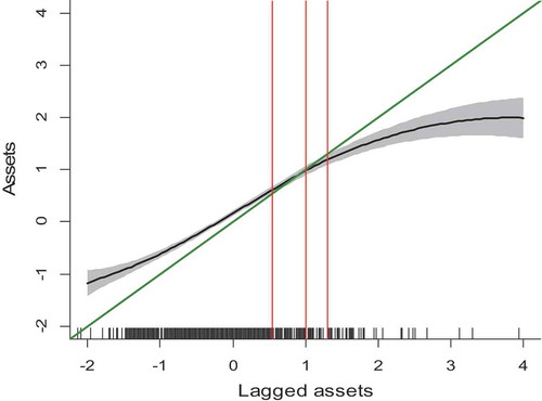
Household asset dynamics based on penalised spline semiparametric regression. Note: Vertical lines represent (from left to right) the lower bound of the confidence interval, the stable equilibrium point, and the upper bound of the confidence interval.

Appendix D.

Binary probit model to test for non-random attrition (from observables)

Table

	2009		2012
	(1)	(2)	(3)	(4)
Total income^a	0.080 (0.120)	0.040 (0.130)	0.240* (0.130)	0.190 (0.120)
Head education	0.001 (0.026)		0.019 (0.024)
Maxmum household education	−0.061** (0.026)		−0.043* (0.025)
Number of male adults	0.018 (0.083)		0.038 (0.077)
Number of female adults	−0.139 (0.093)		−0.146 (0.094)
Value of implements^a	−0.050 (0.350)		0.150 (0.330)
Area of land owned (sqm) ^a	−11.300** (5.000)		−9.500** (4.600)
Total value of livestock^a	0.020 (0.040)		0.003 (0.040)
Value of jewelry^a	0.120 (0.090)		0.090 (0.100)
Bank saving^a	−0.190 (0.189)		−0.220 (0.180)
Asset index, P1		−0.094 (0.067)		−0.072 (0.065)
Asset index, P2		−0.194*** (0.064)		−0.107* (0.060)
Debt^a	0.440*** (0.160)	0.500*** (0.160)	0.420** (0.170)	0.440** (0.180)
HHead age	0.002 (0.008)	−0.003 (0.007)	0.004 (0.007)	−0.003 (0.007)
Head sex	0.248 (0.248)	0.070 (0.228)	0.325 (0.234)	0.140 (0.216)
Head born in the village	0.223 (0.206)	0.236 (0.202)	−0.140 (0.198)	−0.106 (0.191)
Head belong to the biggest ethnic group	−0.121 (0.185)	−0.171 (0.178)	−0.084 (0.168)	−0.122 (0.162)
Head married	−0.220 (0.213)	−0.205 (0.206)	−0.132 (0.199)	−0.146 (0.194)
Number of children	−0.147** (0.064)	−0.133** (0.062)	−0.113* (0.059)	−0.099* (0.058)
Number of elders	0.141 (0.157)	0.133 (0.147)	0.231 (0.150)	0.248* (0.136)
Shock (moderate)	−0.201 (0.195)	−0.185 (0.192)	−0.117 (0.174)	−0.107 (0.170)
Shock (severe)	−0.012 (0.243)	0.099 (0.235)	−0.121 (0.237)	−0.008 (0.226)
Chitwan	−0.349 (0.255)	−0.294 (0.239)	−0.501** (0.232)	−0.453** (0.218)
Kaski	−0.424 (0.304)	−0.325 (0.285)	−0.394 (0.272)	−0.274 (0.254)
Constant	0.636 (0.749)	−0.095 (0.700)	0.160 (0.711)	−0.139 (0.653)
Neither laughed nor smiled	−0.214 (0.542)	−0.172 (0.538)	−0.076 (0.543)	−0.063 (0.524)
Only smiled	−0.714 (0.522)	−0.669 (0.517)	−0.423 (0.523)	−0.404 (0.508)
Smiled and laughed	−1.002* (0.521)	−0.934* (0.512)	−0.692 (0.515)	−0.677 (0.498)
Laughed openly and frequently	−0.484 (0.505)	−0.447 (0.503)	−0.209 (0.510)	−0.198 (0.495)
Joint test of instruments χ^2(4)	12.690**	12.600**	10.170**	10.790**
Joint test of model χ^2 (27) for (1)and χ^2 (20) for (2)	56.700***	46.680***	58.060***	40.380***
Pseudo R2	0.142	0.113	0.120	0.091
# Observations	505	505	505	505

Notes: NB: Values in parenthesis are standard errors; ***1 per cent significance, **5 per cent significance, *10 per cent significance. One observation excluded due to missing instrument information and another one due to implausibly high total income value. Individual asset variables included instead of the asset indices generated based on PCA. ^aValues that are rescaled: the original values are divided by 100,000.

Appendix E.

Test for the presence of attrition bias (from observables)

Table

				Total income		P1	P2
2009	‘non-attritors’ vs ‘entire’ sample	Slope parameters	χ^2 (19)^a	12.36 (0.870)	χ^2 (10)^a	12.74 (0.239)	12.01 (0.284)
		All parameters	χ^2 (20)^b	13.44 (0.900)	χ^2 (11)^b	14.21 (0.222)	15.99 (0.142)
	‘non-attritors’ vs ‘attritors’ sample	Slope parameters	χ^2 (19)^c	19.28 (0.439)	χ^2 (10)^c	14.69 (0.144)	17.89** (0.057)
		All parameters	χ^2 (20)^d	19.35 (0.450)	χ^2 (11)^d	16.45 (0.125)	22.61** (0.020)
2012	‘non-attritors’ vs ‘entire’ sample	Slope parameters	χ^2 (19)^a	14.64 (0.745)	χ^2 (10)^a	12.83 (0.234)	14.68 (0.144)
		All parameters	χ^2 (20)^b	14.65 (0.796)	χ^2 (11)^b	12.85 (0.303)	16.32 (0.130)
	‘non-attritors’ vs ‘attritors’ sample	Slope parameters	χ^2 (19)^c	27.72* (0.090)	χ^2 (10)^c	17.22* (0.070)	20.10** (0.028)
		All parameters	χ^2 (20)^d	28.51* (0.098)	χ^2 (11)^d	17.24 (0.101)	21.78** (0.026)

Notes: NB: Values in parenthesis are p-values. ***1 per cent significance, **5 per cent significance, *10 per cent significance. ^aTest of the null hypothesis that slope coefficients are equal between ‘non-attritors’ and ‘entire’ samples. ^bTest of the null hypothesis that all coefficients (including the constant term) are equal between ‘non-attritors’ and ‘entire’ samples. ^cTest of the null hypothesis that slope coefficients are equal between ‘non-attritors’ and ‘attritors’ samples. ^dTest of the null hypothesis that slope coefficients (including the constant term) are equal ‘non-attritors’ and ‘attritors’ samples.

Appendix F.

Household asset dynamics based on livelihood-weighted approach; vertical lines represent (from left to right) the stable equilibrium point and the stable asset equilibrium point.

References

- Abro, Z. A., Alemu, B. A., & Hanjra, M. A. (2014). Policies for agricultural productivity growth and poverty reduction in rural Ethiopia. World Development, 59, 461–474.
- Adams Jr., R. H. (1998). Remittances, investment, and rural asset accumulation in Pakistan. Economic Development and Cultural Change, 47, 155–173.
- Adato, M., Carter, M. R., & May, J. (2006). Exploring poverty traps and social exclusion in South Africa using qualitative and quantitative data. Journal of Development Studies, 42, 226–247.
- Adhikari, B., Di Falco, S., & Lovett, J. C. (2004). Household characteristics and forest dependency: Evidence from common property forest management in Nepal. Ecological Economics, 48, 245–257.
- Amarasinghe, U., Samad, M., & Anputhas, M. (2005). Spatial clustering of rural poverty and food insecurity in Sri Lanka. Food Policy, 30, 493–509.
- Angelsen, A., Jagger, P., Babigumira, R., Belcher, B., Hogarth, N. J., Bauch, S., … Wunder, S. (2014). Environmental income and rural livelihoods: A global-comparative analysis. World Development, 64, S12–S28.
- Angelsen, A., & Wunder, S. (2003). Exploring the forest-poverty link: Key concepts, issues and research implications. Bogor, Indonesia: CIFOR, Center for International Forestry Research.
- Babulo, B., Muys, B., Nega, F., Tollens, E., Nyssen, J., Deckers, J., & Mathijs, E. (2009). The economic contribution of forest resource use to rural livelihoods in Tigray, Northern Ethiopia. Forest Policy and Economics, 11, 109–117.
- Banerjee, A. V., and Duflo, E. (2011). Poor economics: A radical rethinking of the way to fight global poverty. New York, NY: PublicAffairs.
- Barbier, E. B. (2010). Poverty, development, and environment. Environment and Development Economics, 15, 635–660.
- Barrett, C. B., Garg, T., & McBride, L. (2016). Well-being dynamics and poverty traps. Annual Review of Resource Economics, 8, 303–327.
- Barrett, C. B., Marenya, P. P., McPeak, J. G., Minten, B., Murithi, F., Oluoch-Kosura, W., … Wangila, J. (2006). Welfare dynamics in rural Kenya and Madagascar. The Journal of Development Studies, 42, 248–277.
- Bigsten, A., & Shimeles, A. (2008). Poverty transition and persistence in Ethiopia: 1994-2004. World Development, 36, 1559–1584.
- Burke, W. J., & Jayne, T. S. (2008). Spatial disadvantages or spatial poverty traps: Household evidence from rural Kenya (MSU International Development Working Paper #93). Michigan: Michigan State University.
- Byron, N., & Arnold, M. (1999). What futures for the people of the tropical forests? World Development, 27, 789–805.
- Carter, M. R., & Barrett, C. B. (2006). The economics of poverty traps and persistent poverty: An asset-based approach. The Journal of Development Studies, 42, 178–199.
- Carter, M. R., Little, P. D., Mogues, T., & Negatu, W. (2007). Poverty traps and natural disasters in Ethiopia and Honduras. World Development, 35, 835–856.
- Cavendish, W. (2002). Quantitative methods for estimating the economic value of resource use to rural livelihoods. In B. M. Campbell & M. K. Luckert (Eds.), Uncovering the hidden harvest: Valuation methods for woodland and forest resources (pp. 17–65). London: Earthscan.
- CBS. (2013). Environmental statistics of Nepal. Kathmandu: Nepal Central Bureau of Statistics. Retrieved from http://apps.unep.org/publications/pmtdocuments/-Environment_Statistics_of_Nepal,_2013-2014Nepal_EnvironmentStatistics_2013.pdf.pdf
- Charlery, L., & Walelign, S. Z. (2015). Assessing environmental dependence using asset and income measures: Evidence from Nepal. Ecological Economics, 118, 40–48.
- CIFOR. (2007). PEN technical guidelines. Bogor, Indonesia: Author.
- Dercon, S., & Krishnan, P. (2000). Vulnerability, seasonality and poverty in Ethiopia. Journal of Development Studies, 36, 25–53.
- Djoudi, H., Vergles, E., Blackie, R. R., Koffi Koame, C., & Gautier, D. (2015). Dry forests, livelihoods and poverty alleviation: Understanding current trends. International Forestry Review, 17, 54–69.
- Filmer, D., & Pritchett, H. (2001). Estimating wealth effects without data or tears: An application to educational enrollment in states of India. Demography, 38, 115–132.
- Fisher, M., & Shively, G. (2005). Can income programs reduce tropical forest pressure? Income shocks and forest use in Malawi. World Development, 33, 1115–1128.
- Foster, W., Valdés, A., Davis, B., & Anríquez, G. (2011). The constraints to escaping rural poverty: An analysis of the complementarities of assets in developing countries. Applied Economic Perspectives and Policy, 33(4), 528–565.
- Franzel, S., Carsan, S., Lukuyu, B., Sinja, J., & Wambugu, C. (2014a). Fodder trees for improving livestock productivity and smallholder livelihoods in Africa. Current Opinion in Environmental Sustainability, 6, 98–103.
- Franzel, S., Kiptot, E., & Lukuyu, B. (2014b). Agroforestry: Fodder trees. Encyclopedia of Agriculture and Food Systems, 1, 235–243.
- Giesbert, L., & Schindler, K. (2012). Assets, shocks, and poverty traps in rural Mozambique. World Development, 40, 1594–1609.
- Haddad, L., & Ahmed, A. (2003). Chronic and transitory poverty: Evidence from Egypt, 1997–99. World Development, 31, 71–85.
- Hogarth, N., Belcher, B., & Campbell, B. (2013). The role of forest-related income in household economies and rural livelihoods in the border-region of Southern China. World Development, 43, 111–123.
- IFAD. 2013. Enabling poor rural people to overcome poverty in Nepal. Retrieved from http://www.ifad.org/operations/projects/regions/pi/factsheets/nepal.pdf
- Iiyama, M., Kariuki, P., Kristjanson, P., Kaitibie, S., & Maitima, J. (2008). Livelihood diversification strategies, incomes and soil management strategies: A case studyfrom Kerio Valley, Kenya. Journal of International Development, 20, 380–397.
- Iversen, V., Chhetry, B., Francis, P., Gurung, M., Kafle, G., Pain, A., & Seeley, J. (2006). Hidden value forests, hidden economies and elite capture: Evidence from forest user groups in Nepal's Terai. Ecological Economics, 58, 93–107.
- Jalan, J., & Ravallion, M. (1997). Spatial poverty traps? (World Bank Policy Research Working Paper # 1862). Washington, DC: World Bank.
- Jiao, X., Pouliot, M., & Walelign, S. Z. (2017). Livelihood strategies and dynamics in rural Cambodia. World Development, 93, 266–278.
- Jiao, X., Walelign, S. Z., Nielsen, M., R. & Smith-Hall, C. (2019). Protected areas, household environmental incomes and well-being in the Greater Serengeti-Mara Ecosystem. Forest Policy and Economics, 106, 101948.
- Jones, S. 2016. Social causes and consequences of energy poverty. In K. Csiba (Ed.), Energy poverty handbook. Brussels: European Union.
- Kam, S.-P., Hossain, M., Bose, M. L., & Villano, L. S. (2005). Spatial patterns of rural poverty and their relationship with welfare-influencing factors in Bangladesh. Food Policy, 30, 51–567.
- Krishna, A. (2007). For reducing poverty faster: Target reasons before people. World Development, 35, 1947–1960.
- Larsen, H. O., Rayamajhi, S., Chhetri, B. B. K., Charlery, L. C., Gautam, N., Khadka, N., … Walelign, S. Z. (2014). The role of environmental incomes in rural Nepalese livelihoods 2005 – 2012: Contextual information (Vol. 79). Copenhagen: Department of Food and Resource Economics, University of Copenhagen.
- Lybbert, T. J., Barrett, C. B., Desta, S., & Coppock, D. L. (2004). Stochastic wealth dynamics and risk management among a poor population. Economic Journal, 114, 750–777.
- Maskay, N. M., & Adhikari, S. R. (2013). Remittances, migration and inclusive growth: The case of Nepal (ARTNeT Policy Brief #.35). Bangkok: United Nations ESCAP.
- May, J., & Woolard, I. (2007). Poverty traps and structural poverty in South Africa: Reassessing the evidence from KwaZulu-Natal. Chronic Poverty Research Center Working Paper #82.
- McSweeney, K. 2004. Forest product sale as natural insurance: The effects of household characteristics and the nature of shock in eastern Honduras. Society and Natural Resources 17: 39–56.
- Meilby, H., Puri, L., Christensen, M., & Rayamajhi, S. (2006). Planning a system of permanent sample plots for integrated long-term studies on community-based forest management. Banko Janakari, 16(2), 3–11.
- Naschold, F. (2012). The poor stay poor: Household asset poverty traps in rural semi-arid India. World Development, 40, 2033–2043.
- Naschold, F. (2013). Welfare dynamics in Pakistan and Ethiopia – Does the estimation method matter? The Journal of Development Studies, 49, 936–954.
- Nielsen, Ø. J., Rayamajhi, S., Uberhuaga, P., Meilby, H., & Smith-Hall, C. (2013). Quantifying rural livelihood strategies in developing countries using an activity choice approach. Agricultural Economics, 44, 57–71.
- Nightingale, A. (2003). Nature-society and development: Social, cultural and ecological change in Nepal. Geoforum, 34(4), 525–540.
- Pattanayak, S. K., & Sills, E. O. (2001). Do tropical forests provide natural insurance? The microeconomics of non-timber forest product collection in the Brazilian Amazon. Land Economics, 77, 595–613.
- Pouliot, M., Pyakurel, D., & Smith-Hall, C. (2018). High altitude organic gold: The production network for Ophiocordyceps sinensis from far-western Nepal. Journal of Ethnopharmacology, 218, 59–68.
- Pouliot, M., & Treue, T. (2013). Rural people’s reliance on forests and the non-forest environment in West Africa: Evidence from Ghana and Burkina Faso. World Development, 43, 180–193.
- Pyakurel, D., Bhattarai, I., & Smith-Hall, C. (2018). Patterns of change: The dynamics of medicinal plants trade in far-western Nepal. Journal of Ethnopharmacology, 224, 323–334.
- Quisumbing, A. R., & Baulch, B. (2013). Assets and poverty traps in rural Bangladesh. The Journal of Development Studies, 49, 898–916.
- Rasul, G., Karki, M., & Sah, R. P. (2008). The role of non-timber forest products in poverty reduction in India: Prospects and problems. Development in Practice, 18, 779–788.
- Reddy, S. R. C., & Chakravarty, S. P. (1999). Forest dependence and income distribution in a subsistence economy: Evidence from India. World Development, 27, 1141–1149.
- Roe, D., Elliott, J., Sandbrook, C., & Walpole, M. (2013). Tackling global poverty: What contribution can biodiversity and its conservation really make? In D. Roe, J. Elliott, C. Sandbrook, & M. Walpole (Eds.), Biodiversity conservation and poverty alleviation: Exploring the evidence for a link (pp. 316–328). UK: Wiley-Blackwell.
- Santos, P., & Barrett, C. B. (2006). Informal insurance in the presence of poverty traps: Evidence from southern Ethiopia. In Annual meeting of the international association of agricultural economists, Queensland.
- Scharlemann, J. P. W., Mant, R. C., Balfour, N., Brown, C., Burgess, N. D., Guth, M., … Kapos, V. (2016). Global goals mapping: The environment-human landscape. A contribution towards the NERC, the Rockefeller Foundation and ESRC initiative, towards a sustainable Earth: Environment-human systems and the UN global Goals. Cambridge, UK: Sussex Sustainability Research Programme, University of Sussex, Brighton, UK and UN Environment World Conservation Monitoring Centre.
- Shackleton, C. M., Shackleton, S. E., Buiten, E., & Bird, N. (2007). The importance of dry woodlands and forests in rural livelihoods and poverty alleviation in South Africa. Forest Policy and Economics, 9, 558–577.
- Skoufias, E. (2003). Economic crises and natural disasters: Coping strategies and policy implications. World Development, 31, 1087–1102.
- Tesfaye, Y., Roos, A., Campbell, B. M., & Bohlin, F. (2011). Livelihood strategies and the role of forest income in participatory-managed forests of Dodola area in the bale highlands, southern Ethiopia. Forest Policy and Economics, 13, 258–265.
- Thagunna, K. S., & Acharya, S. (2013). Empirical analysis of remittance inflow : The case of Nepal. International Journal of Economics and Financial Issues, 3, 337–344.
- Thieme, S., & Wyss, S. (2005). Migration patterns and remittance transfer in Nepal: A case study of Sainik Basti in Western Nepal. International Migration, 43(5), 59–98.
- Vedeld, P., Angelsen, A., Sjaastad, E., & Berg, G. K. (2004). Counting on the environment: Forest income and the rural poor. EDP 98. Washington, DC: World Bank.
- Vira, B., & Kontoleon, A. (2013). Dependence of the poor on biodiversity: Which poor, what biodiversity? In D. Roe, J. Elliott, C. Sandbrook, & M. Walpole (Eds.), Biodiversity conservation and poverty alleviation: Exploring the evidence for a link (pp. 52–84). Wiley-Blackwell.
- Walelign, S. Z. (2013). Forests beyond income: The contribution of forest and environmental resources to poverty incidence, depth and severity. International Journal of AgriScience, 3, 533–542.
- Walelign, S. Z. (2016a). Should all attrition households in rural panel datasets be tracked? Lessons from a panel survey in Nepal. Journal of Rural Studies, 47, 242–253.
- Walelign, S. Z. (2016b). Livelihood strategies, environmental dependency and rural poverty: The case of Mozambique. Environment. Development and Sustainaibility, 18, 593–613.
- Walelign, S. Z., Charlery, L., Smith-Hall, C., Chhetri, B. B. K., & Larsen, H. O. (2016). Environmental income improves household-level poverty assessments and dynamics. Forest Policy and Economics, 71, 23–35.
- Walelign, S. Z., Nielsen, M. R., & Larsen, H. O. (2019). Environmental income as a pathway out of poverty? Empirical evidence on asset accumulation in Nepal. Journal of Development Studies, 55, 1508–1526.
- Winters, P., Davis, B., Carletto, G., Covarrubias, K., Quiñones, E. J., Zezza, A., … Stamoulis, K. (2009). Assets, activities and rural income generation: Evidence from a multicountry analysis. World Development, 37, 1435–1452.
- Wong, G. Y., & Godoy, R. (2003). Consumption and vulnerability among foragers and horticulturalists in the rainforest of Honduras. World Development, 31(8), 1405–1419.
- Wunder, S., Luckert, M., & Smith-Hall, C. (2011). Valuing the priceless: What are non-marketed products worth? In A. Angelsen, H. O. Larsen, J. F. Lund, C. Smith-Hall & S. Wunder (Eds.), Measuring livelihoods and environmental dependence: Methods for research and fieldwork (pp. 127–145). London: Earthscan.
- Yemiru, T., Roos, A., Campbell, B. M., & Bohlin, F. (2010). Forest incomes and poverty alleviation under participatory forest management in the Bale Highlands, Southern Ethiopia. International Forestry Review, 12(1), 66–77.
- Zimmerman, F., & Carter, M. R. (2003). Asset smoothing, consumption smoothing and the reproduction of inequality under risk and subsistence constraints. Journal of Development Economics, 71, 233–260.