The Impact of Road Development on Household Welfare in Rural Papua New Guinea

Abstract

In this paper we evaluate the impact of road development on household welfare in rural Papua New Guinea (PNG) between 1996 and 2010, using two geocoded cross-sectional national household surveys and corresponding road maps. We make use of time-variation in road surface type and condition as recorded in PNG’s National Road Asset Management System, focusing on routes that connect rural households to urban areas. To tackle endogenous placement of road infrastructure programs, we employ a correlated random effects model that controls for the location-specific average road quality over the period of analysis. We also use a newly developed generalised quantile regression method to investigate whether road works favour the poor. Our estimates show that better roads to nearest towns lead to higher consumption levels and housing quality, and to less reliance on subsistence farming. The effects are stronger among poor and remote households.

Keywords:

• Rural roads
• infrastructure
• household welfare
• social issues
• poverty
• Papua New Guinea

1. Introduction

Road access is one of the key elements necessary for rural economic development, generally offering the sole means for connecting people to markets and public services. Better roads connect rural households to goods and labour markets, providing a greater variety and lower prices of essential inputs and consumption goods, as well as higher prices and demand for local products (Gibson & Rozelle, 2003). Increased market access may raise local productivity and wages, and enable the transformation from subsistence agriculture to growing cash crops and to non-agricultural activities, thus diversifying household income sources (Aggarwal, 2018; Mu & van de Walle, 2011). Better roads may also attract financial service providers, facilitating agricultural investments and consumption smoothing (Binswanger, Khandker, & Rosenzweig, 1993), and enhance access to and quality of services like schools and hospitals (Bell & van Dillen, 2014).

Each of these factors suggests that better roads lead to higher average household consumption, which is confirmed by several studies (Knox, Daccache, & Hess, 2013). The distributional effects of better roads, however, are less understood, and the relative benefits to poor households are unclear. If better-off households are more able to compensate a lack of good roads –say, because they can better smooth out their consumption during seasons where roads are not usable, or through access to four-wheel drives – the poor would experience a relatively higher productivity gain from improved roads. Conversely, non-poor households may benefit more from better roads, since they might be able to scale up agricultural production more easily, or because the poor may be kept from road utilization due to transport costs. The effects of roads on other development outcomes beside consumption are also ambiguous. Non-agricultural employment may increase or decrease as a result of better roads, depending on the relative change in agricultural productivity. School enrolment may increase or decrease, depending on how infrastructure changes education returns and the opportunity cost of schooling (Adukia, Asher, & Novosad, 2020).

In this paper, we investigate the effect of road quality on household welfare in rural Papua New Guinea (PNG) between 1996 and 2010. PNG is a good case study ground for the effects of rural infrastructure development, due to its limited road access and high variability in road quality. In 2009, the country had a road density of 56 km per 1000 km², which is very low compared to other countries in the region (neighbouring Indonesia had 250 km per 1,000 km²). In the same year, only 13% of roads were sealed, while the majority of roads were gravel or dirt roads.

We combine two household surveys with censuses as well as GIS datasets of the road network from the time the household surveys were administered. The road map data contains measures of surface type and condition for each road section of 100 m. Together with the location of households, we can calculate the distance to the nearest road, and the quality and length of the shortest route leading to the nearest town. This allows us to construct a set of road variables that captures quality at a very granular level, considering not just the section proximate to the households but arguably the most important road for each household in its entirety.

We use six indicators for household welfare: consumption, poverty status, household engagement in subsistence farming, wage employment, housing quality, and school enrolment. Our results suggest that access to better roads increases consumption and reduces poverty by facilitating the transition out of subsistence farming and into more market-based agriculture. Access to better roads leads to a higher probability of living in a house made of non-traditional material, and greater likelihood that children are enrolled in school. We also find that disadvantaged and more remote households benefit comparatively more from upgraded roads.

To identify the impact of road quality on the route that leads to the nearest town, we use a correlated random effects model to account for endogeneity of road quality. Following the approach by Mundlak (1978), we correct for unobserved location-specific effects by including the average of the road quality variables obtained from the two maps. The resulting estimator is identical to the within estimator, despite the absence of panel data. Our results generally point to beneficial effects of sealing roads. The estimates suggest that, between 1996 and 2010, upgrading 1 km of the route leading to the nearest town from dirt to sealed road surface increased average household consumption by about 3.2%, raised the chance households lived in a house with a high-quality roof by about 1.3 percentage points, reduced the probability a household relied on subsistence farming by 0.5 percentage points, and increased the likelihood for a school-aged child to be enrolled in school by 1.4 percentage points.

We also explore effect heterogeneity. Our model is run on several population subgroups to see how the effect of road quality on consumption and poverty varies by remoteness of the household, its education level, and its demographic characteristics. We find that the effects on consumption and poverty are at least twice as high for households living more than 30 km from the nearest town, when compared to those living closer than 30 km. In addition, we apply a generalised quantile regression estimator (Powell, 2020) to investigate how the effects of road infrastructure vary across the consumption distribution. This procedure allows us to examine how different consumption quantiles are affected while also accounting for covariates, making the results comparable to the results from our base specification. Our estimates weakly indicate that the effect of upgrading dirt roads is higher for the poorest households, suggesting that road works can be considered anti-poverty measures in the case of rural PNG.

The remainder of the paper is structured as follows. In section 2 we discuss the related literature on roads and household welfare, and the associated methodological challenges. In section 3 we give the country context of the study and explain the data we use. Section 4 outlines the estimation techniques we use. In section 5 we present and discuss estimation results. In section 6 we offer some concluding points.

2. Literature

Estimating the impact of roads is complicated by the fact that government decisions about where to construct new roads, or whether to rehabilitate or upgrade existing ones, are likely correlated with areas’ growth and other development achievements. These decisions are often made based on unobserved factors like expected traffic volume, local productivity, investment cost, and political benefits of placing roads in particular areas – all factors that may also affect household welfare directly (see e.g. Burgess, Jedwab, Miguel, Morjaria, & Padró i Miquel, 2015).

Existing research on the impact of transport infrastructure has used a variety of approaches to address this endogeneity problem. Instrumental variable estimation – which requires an exogenous variable that affects road development but has no direct effect on the outcome variable of interest – is one approach. Gibson and Rozelle (2003), who also study the impacts of road infrastructure in PNG, use the year in which the national highway system penetrated the district as an instrument. A related method uses the distance from a hypothetical connection between historical centres, such as straight lines or routes predicted based on geography, as an instrument. Areas close to the connection have a higher chance of being connected to the road network, while this distance is arguably not a causal factor for economic development. This approach has been followed to obtain impact estimates of transport infrastructure in China (Banerjee, Duflo, & Qian, 2020) and Nepal (Shrestha, 2020). Gertler, Gonzalez-Navarro, Gračner, & Rothenberg (2022) instrument district-level road maintenance investments in Indonesia by interacting province budgets with characteristics from other districts, exploiting the fact that resource allocation from the central government to provinces follows a strict rule set. Regression discontinuity designs have been used to study road impacts where investment decisions were made based on whether localities exceeded a threshold at some priority measure. Examples include program evaluations in Sierra Leone (Casaburi, Glennerster, & Suri, 2013) and India (Adukia et al., 2020, Asher & Novosad, 2020; Aggarwal, 2018). A technique often used for binary road variables is difference-in-differences estimation, sometimes combined with propensity score matching to allow the common trend assumption to hold conditional on covariates (Lokshin & Yemtsov, 2005; Mu & van de Walle, 2011).

Where panel data is available, another approach to address potential endogeneity in road works is to use village or household fixed effects (Gibson & Olivia, 2010; Khandker, Bakht, & Koolwal, 2009; Khandker & Koolwal, 2010) to assess the impact of road investments over the period covered by the panel. The fixed effects approach accounts for endogeneity caused by time-invariant characteristics of the location. The availability of multiple time periods further allows instrumentation using lagged outcomes (Dercon, Gilligan, Hoddinott, & Woldehanna, 2009; Khandker & Koolwal, 2011). The studies mentioned here all require that the same households are interviewed repeatedly over a time span sufficiently long to measure the impact of road investments. However, our study only uses repeated cross-sectional data, in conjunction with repeated measurements for road variables. Using the Mundlak (1978) estimator, we apply a correlated random effects model to incorporate village fixed effects. That makes our approach applicable in a broad range of settings where panel data is not available.

Only a few studies have examined heterogeneity in the impacts of roads. Dercon et al. (2009) find that access to an all-weather road in rural Ethiopia between 1994 and 2004 reduced poverty by 6.9 percentage points. They find no evidence of heterogeneity of this effect across household characteristics like size of landholdings, livestock holdings, or literacy of the household head. However, their estimates show the effect on consumption growth is larger for households with landholdings of at least a hectare and a literate household head. Dercon, Hoddinott, and Woldehanna (2012) obtain complementary results, finding that remoteness from towns and poor roads are among the factors most associated with chronic poverty. Khandker et al. (2009) investigate how households in Bangladesh profited from road improvement projects. They predict that villages next to an improved road experience a poverty reduction of 3–6 percentage points over 4 years. The impact on household expenditure is higher for lower expenditure quintiles in this study, suggesting that road investments are pro-poor. However, using a larger dataset and controlling for other investment programs, Khandker and Koolwal (2010) find the opposite pattern. Mu and van de Walle (2011) find positive and significant average effects of rural road rehabilitation on local market development in Vietnam. The authors note a tendency for poorer localities to have higher impacts due to lower levels of initial market development. A replication study by Nguyen (2019) confirms these results.

3. Data and context

With a population of roughly 8.9 million people in 2020, PNG is the largest and most populated country of the Pacific region. During the years covered by the data used in this study (1996–2010), PNG’s real per capita growth was moderate – averaging 2.6% per year – and poverty incidence even grew by two percentage points to roughly 40% of the population (Gibson, 2012). During that time period, the share of PNG’s population living in rural areas has remained constant at around 87% according to the 2011 census, of which around 90% largely relied on (semi-)subsistence agriculture (see Table 1).

Table 1. Summary statistics for the analysis sample

	1996			2009/2010
	Mean	SD	N	Mean	SD	N	p-Value
Outcomes (PNGHS 96, HIES 09/10)
Log real per adult-equivalent expenditure	0.309	0.560	680	0.157	0.946	1473	0.033
Poverty	0.347	0.376	680	0.429	0.583	1473	0.045
Engaged in subsistence farming	0.889	0.253	680	0.914	0.318	1643	0.399
Someone in the household has wage job	0.243	0.346	680	0.137	0.390	1632	0.003
Home has a good roof	0.244	0.346	680	0.285	0.512	1643	0.205
Ratio of children aged 7–17 going to school	0.445	0.325	484	0.589	0.491	1054	0.000
Location-specific control variables (PNGRIS)
Altitude (m)	1003	595	680	1185	951	1643	0.013
Dummy, slope > 10 degrees	0.634	0.388	680	0.664	0.536	1643	0.718
Dummy, land inundation occurs	0.236	0.342	680	0.240	0.485	1643	0.955
Dummy, rainfall deficit is rare	0.290	0.366	680	0.322	0.530	1643	0.695
Annual rainfall (m)	2.640	0.513	680	2.650	0.813	1643	0.929
Log population nearest town (Census)	8.615	1.007	680	8.805	1.407	1643	0.374
Household controls (PNGHS 96, HIES 09/10)
Household size	5.839	2.438	680	4.906	2.785	1643	0.000
Ratio of household members under 15	0.406	0.208	680	0.352	0.263	1643	0.000
Ratio of household members above 50	0.104	0.172	680	0.127	0.268	1643	0.117
Age of household head	40.75	10.32	680	42.47	15.61	1643	0.032
Household head is female	0.094	0.235	680	0.148	0.402	1643	0.006
Household head is literate	0.525	0.403	680	0.473	0.567	1642	0.192
Average years of schooling	3.392	2.389	680	4.373	3.993	1633	0.000
Ratio of children in primary school age	0.602	0.302	484	0.583	0.433	1054	0.469
Impact variables (obtained from road maps)
Distance to nearest road (km)	0.609	1.234	680	0.907	2.141	1643	0.262
Distance on road to nearest town (km)	49.99	39.03	680	36.57	39.07	1643	0.044
Road to town: km of sealed road	16.10	21.15	680	14.68	28.48	1643	0.751
Road to town: km of gravel road	30.47	27.67	680	17.69	24.67	1643	0.007
Road to town: km of dirt road	3.428	6.206	680	4.199	10.92	1643	0.589

Notes: Summary statistics of log real per adult-equivalent expenditure and poverty are obtained using person sampling weights. All other ones are obtained using household sampling weights. Standard deviations and p-values account for clustering at the village level. The p-values show the probability of equal means.

Development and maintenance of PNG’s road network suffered during the two decades following independence, when funding for road maintenance fell by half (Kwa, Howes, & Lin, 2010). Government expenditure on infrastructure per capita reached its minimum in 2001, but large and sustained increases in funding only began in 2010 (Dornan, 2016). Beside low government revenues, several other factors have made it difficult to build and maintain roads during this period: limited road management capacity in the private sector due to unsteady provision of maintenance contracts, competition for construction equipment and skilled engineers between resource extraction enterprises and the Department of Works, and disputes with owners of land proximate to road works (Lucius, 2010). Alongside these practical obstacles to implementation, a lack of political will due to the low visibility of road investments, as well as high levels of corruption contributed to the insufficient maintenance of the road network (Dornan, 2016). Lastly, PNG’s climate and geography, with its rugged topography, seismic activity, intense weathering, and high seasonal rainfall in many regions – especially in the densely populated agricultural heartland of the Highlands region – make road construction and maintenance challenging (Stead, 1990).

Two nationally representative cross-sectional household surveys conducted in PNG – the 1996 Papua New Guinea Household Survey (PNGHS 96) and the 2009–2010 Household Income and Expenditure Survey (HIES 09/10) – provide the primary source of data on household consumption and other indicators used in this study. The 1996 household survey included a nationally representative sample of 830 rural households in 73 census units (villages). The 2009 survey collected information from 2208 rural households in 125 villages. We also make use of variables from the PNG Census 2000 Community Profile System (CPS 2000), which contains information on the location and population of all villages and towns from the census of 2000. This allows us to locate all the villages in the two surveys as points on a map.¹ The HIES 09/10 includes GPS coordinates of all surveyed households, allowing us to calculate fairly precise household-specific distances to the nearest road. In addition, we make use of the Papua New Guinea Resource Information System (PNGRIS) of the PNG National Agricultural Research Institute (Bryan & Shearman, 2008). This spatial database contains information on elevation, climate, and other biophysical characteristics which we include as control variables in our analysis.

For data on the status of road infrastructure over time, we rely on the road information data bank and the geographical information system of the Road Asset Management System (RAMS). The RAMS project, initiated in 1998 by the PNG Department of Works (DoW), was designed to provide a road database and analytical tool to inform policy makers about road needs and economic efficiency of investments in the road network (Jusi, Mumu, Jarvenpaa, Neausemale, & Sangrador, 2003). We link initial RAMS data – based on road surveys conducted between 1999 and 2001 – to the PNGHS 96 (we refer to the combined data as the 2000 map). Due to continued underinvestment in the transport sector, certain dimensions of the RAMS – particularly its traffic counts (vital to estimating a road’s value) – were not updated after 2001. However, the provincial works managers of the DoW were given financial support to update data on road quality, and data collected by DoW provide the basis for our dataset of roads in 2009. The road system consisted of roughly 26,000 km of roads in 2009. We link this dataset to the HIES 09/10 and refer to it as the 2009 map.²

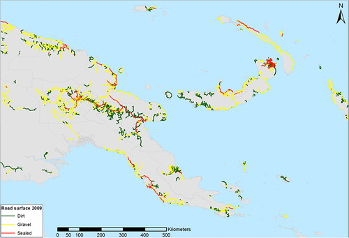
Both the 2000 and 2009 road maps include detailed information for each road segment. Most importantly, surface type (sealed, gravel, dirt) and condition (good, fair, poor) are given for all segments. The 2009 road map has much more extensive coverage of the road network – covering an additional 14,000 km of roads not included in the 2000 map, consisting mostly of gravel or dirt feeder roads. However, within our study period the focus of road works in PNG was on maintenance and upgrading, and reportedly no new roads were constructed during this period (World Food Programme & Logistics Cluster 2011; also confirmed in discussions with informants at the DoW). This leads us to conclude that the higher density of roads depicted in the 2009 map is a result of an improvement of the information contained in the map, rather than the construction of new roads.

Figures 1 and 2 map the roads, distinguished by surface type, comprising identified stretches of the national network in 2000 and 2009. A comparison of the maps shows that most of the missing road segments in 2000 are classified as dirt roads in 2009. This is partly because the additional roads on the 2009 map are made up almost entirely of provincial roads, which were more likely to have a dirt surface than national roads. In the online appendix we show descriptive statistics of the road network for both years, as well as transition matrices of surface type and condition for those roads included in both maps. They do not reveal an apparent trend in road status, in that the length of roads upgraded or improved is roughly offset by roads that deteriorated.

Figure 1. Roads by surface type in 2000.

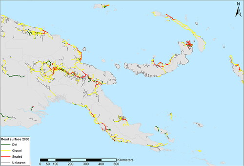
Figure 2. Roads by surface type in 2009.

Using data from the road maps and household surveys, we construct variables indicating the length, surface types and condition of the road leading to the nearest town for the sampled households. We consider the shortest route to the nearest town from the stretch of road that is closest to the household. This route may not be a perfect representation for the roads used by surveyed households – as sometimes the nearest town may not be the most relevant – but we believe that it is a useful heuristic nonetheless. For this route, we calculate the distance for each type of surface and road condition.³ For our analysis, we focus on households that are connected to a town by a road. We exclude households that are located more than 15 km from any road as it seems unlikely that they use the nearest road regularly, making road quality unlikely to have a significant impact. Furthermore, we consider only towns that had more than 1000 inhabitants according to the census 2011 and are within 5 km of the nearest road.⁴ Taken together, these restrictions mean that about 20% of the rural census units in the two surveys are dropped from our analysis. The villages left out are mostly on small islands, in the deep interior in the west of the Momase region, or at the coast of Western province (all of which have a very low population density).

Due to the fact that our road map of 2000 is less detailed than the 2009 map, we have missing information on surface type and condition for some of the road segments of 2000. For the routes used in the analysis, this information was lacking for 24% of the total distance. For that reason, we drop observations where all road segments leading to the nearest town have unknown characteristics for 2000. This leaves a total of 20% of the total distance unknown for 2000. For the remaining observations, we simply assign the segments with unknown characteristics for 2000 the same characteristics as for 2009. We conduct sensitivity checks to examine the implications of this decision, which we discuss in section 5.

Table 1 provides summary statistics for our sample. It includes geographic and road access variables that were merged with the household survey data. Both household surveys include sections that allow calculation of per adult-equivalent household expenditure – based on a closed interval recall method in the PNGHS 96, and on consumption diaries in the HIES 09/10 – as well as regional poverty lines based on the cost of locally consumed foods.⁵ Across the two household surveys, average per adult-equivalent consumption decreased and poverty incidence increased slightly. School enrolment increased by more than 14 percentage points, and average years of schooling of adults increased by almost one year. Households in the 2009/2010 HIES were slightly older (higher average age of household members), smaller (with nearly one person less, on average), and lived closer to the nearest town, compared to the households in the PNGHS 96. These differences could indicate demographic changes but are more likely caused by differences in the sampling schemes for the two surveys. Table 1 also shows the distances by surface type for the routes leading from the sampled households to the nearest town, as measured by us using the road maps and household locations.

We use six different outcome variables in our regressions of road quality. The first one is the same one as used in Gibson and Rozelle (2003): the logarithm of real yearly consumption per adult-equivalent.⁶ We divide yearly consumption by the respective regional rural poverty lines to calculate real consumption. A similar outcome variable is poverty status. We include it as our second outcome to examine specifically how the probability of being poor is affected by road infrastructure.

In addition to consumption, we are also interested in the effects of infrastructure on rural employment and structural transformation. One common change observed among rural households as a result of improved access to markets is reduced dependence on subsistence farming. Therefore, our third outcome is whether members of the household reported engaging in subsistence farming in the days prior to the survey date.⁷ Another indicator of structural change is having a wage job. Accordingly, we use a dummy for whether at least one member of the household is employed in a non-agricultural sector as fourth outcome variable. We expect that better roads improve off-farm earning opportunities and therefore reduce the necessity for subsistence agriculture and increase the likelihood of formal employment.

Another indicator of material well-being is housing quality.⁸ Traditional dwellings, with walls made of bush material and with grass or leaf roofs, are cheap to come by but have a relatively low service life. So, investments in non-traditional housing materials may signify not only an immediate improvement of living conditions but also an intention to stay in a given location more permanently. Due to the lack of credible and intertemporally comparable housing value estimates, we chose to use a dummy indicating whether the house has a good roof, i.e. a roof made of metal, tiles, or cement. If improved road access leads to better opportunities and living conditions and reduces transportation costs, we would expect more good roofs due to better access to roofing materials as well as higher demand for them.

Lastly, we examine the school enrolment ratio of children at school age. Our hypothesis is that school enrolment increases with better road infrastructure due to easier access to schools for both children and teachers.

4. Estimation

To estimate the causal relationship between the quality of the road infrastructure and our outcomes of interest, we propose a linear model of the form (1) $$y_{\mathit{ijt}}=\beta R_{jt}+\gamma D_j+\delta X_{\mathit{ijt}}+{\mu }_j+{\pi }_{pt}+{\epsilon }_{\mathit{ijt}},$$(1) where $y_{\mathit{ijt}}$ is an outcome for household $i$ in village $j$ at time $t,$ $R_{jt}$ and $D_j$ are vectors of variables related to road infrastructure, $X_{\mathit{ijt}}$ is a vector of exogenous control variables (at the household- and the village level), ${\mu }_j$ denotes unobserved, time-invariant heterogeneity at the village level, ${\pi }_{pt}$ is a province time fixed effect, and ${\epsilon }_{\mathit{ijt}}$ is an independent disturbance term.

We include two types of road infrastructure variables. $D_j$ includes the Euclidean distance to the nearest road and the distance on that road leading to the closest town with a 2010 population above 1,000 people. Since we assume no new roads were added between 1996 and 2010, these distance variables are time-invariant. $R_{jt}$ captures the combined length of road segments of a particular type on the route between surveyed households and the nearest town. Since these distances add up to the total distance travelled on that road to the nearest town, which is already included in $D_j,$ we leave out the lowest quality category of road type. This means that the coefficients in $\beta$ give the welfare impact of changing a kilometre of road from the lowest quality type to the other types. Road segments are upgraded, left to deteriorate, or remain the same type over time, so $R_{jt}$ is time-varying.

Since there is no overlap in sampled villages between the two surveys, we cannot difference out the term ${\mu }_j,$ and treating it as a random effect uncorrelated with all independent variables might lead to a biased estimate of $\beta .$ Instead, we use the correlated random effects approach introduced by Mundlak (1978). The idea is to substitute ${\mu }_j$ with the mean of $R_{jt}$ over $t,$ ${\overline{R}}_{j*},$ and an independent village random effect, ${\omega }_j:$ (2) $${\mu }_j=\alpha {\overline{R}}_{j\mathrm{*}}+{\omega }_j.$$(2) $R_{jt}$ is uncorrelated with ${\omega }_j+{\epsilon }_{\mathit{ijt}}.$ This combined disturbance term is also independent between nearby localities, as any spatial correlation is captured by ${\pi }_{pt}$ and ${\overline{R}}_{j*}.$ Since distance variables $D_j$ are time-invariant, they cannot be included in the model of ${\mu }_j$ and are assumed to be conditionally exogenous. The model is estimated using OLS and takes into account the survey design, i.e. sampling weights,⁹ stratum divisions, and standard error clustering by village. To reduce collinearity between the endogenous variables and their respective intertemporal averages, we estimate Equation (1)(1) $$y_{\mathit{ijt}}=\beta R_{jt}+\gamma D_j+\delta X_{\mathit{ijt}}+{\mu }_j+{\pi }_{pt}+{\epsilon }_{\mathit{ijt}},$$(1) using centred terms $R_{jt}-{\overline{R}}_{j*}$ instead of $R_{jt}$ to reflect variables in terms of their deviations from averages over time.

We include several location-specific control variables. Among these are the geoclimatic variables used in Gibson and Rozelle (2003) – namely, altitude (in metres), a dummy for whether the slope is above 10 degrees, a dummy indicating that the land is subject to flooding, a dummy indicating that rainfall deficits are rare, and annual rainfall (in metres). To control for the economic importance of the nearest town, we also include the logarithm of its population as measured in the census closest to the survey year.¹⁰ Population numbers could be endogenous, say, because more productive areas could enhance household welfare as well as faster population growth. To account for this potential source of endogeneity, we include the average of log population in Equation (2)(2) $${\mu }_j=\alpha {\overline{R}}_{j\mathrm{*}}+{\omega }_j.$$(2) .

We also include some household-level controls. This demands caution, however, since changes in road access could alter household characteristics. An example for such an endogenous household variable is the sector of work, which could change as a result of new opportunities created by improved road access, and thus cannot be included. We select a parsimonious set of variables that describes the composition and education level of adults in the household (see Table 1). We report results with and without these household controls for Equation (1)(1) $$y_{\mathit{ijt}}=\beta R_{jt}+\gamma D_j+\delta X_{\mathit{ijt}}+{\mu }_j+{\pi }_{pt}+{\epsilon }_{\mathit{ijt}},$$(1) . Province-time fixed effects are included to control for differences in outcomes due to unobserved factors such as local economic conditions, and the ability and political will to build, maintain, and upgrade roads. They constitute particularly effective controls since the roads to the nearest town, while not having geographical point locations, are for almost all observations located within the same province or at least have the largest part in the province as the corresponding villages. In addition, the province level is where decisions about road rehabilitation, maintenance, and upgrading for non-national roads are being made.

With regard to road types, we explore specifications with different levels of detail. A simple way to capture road quality is to consider only the surface type, i.e. whether a road is sealed, gravelled, or a dirt track. A more detailed categorization of road segments includes surface type together with road condition, i.e. whether a road is in good, fair, or poor shape. In this paper, we only present the results of the analysis using surface type. The more detailed model is consistent with the simpler model but shows no clear effects of road condition, likely due to a lack of statistical power as well as differences in the way road condition was assessed across time and between provinces. The results using road condition can be found in the online appendix.

Our basic model specification rests on the assumption that unobserved factors which both contribute to the respective outcomes and are correlated with road infrastructure are location-specific and fixed over the period between the two surveys. This by itself is a daring presumption given the 13-year period between surveys. Although overall rural economic output and poverty have stagnated over the study period, some areas may have gained or lost in population or economic importance in those years, potentially affecting infrastructure as well as household welfare. We attempt to capture changes in local economic and political conditions by including province-time dummies and year-specific town population numbers. The household level covariates also serve as indicators for economic and demographic conditions at a given time. With these controls, we believe that unobserved time-varying factors are not a cause for concern.

A caveat is that we cannot model selective migration that occurs in response to changes in road quality. This is a potential source of bias for most studies on the benefits of infrastructure; even when panel data is available, the whereabouts of individual migrating household members are seldom recorded. The actual effects of rural road quality on migration are unclear, with some evidence pointing to reduced out-migration (Castaing Gachassin, 2013), while other recent studies find no significant effects (Aggarwal, 2018; Asher & Novosad, 2020). In the online appendix, we look at correlations between our road variables and indicators of migration in PNG, which all turn out small and statistically insignificant. Given this, we believe that selective migration does not bias our estimates to a degree that would invalidate them.

In addition to the average welfare effects of rural roads, we are also interested in whether rural roads affect all households in the same manner. One open question is whether high education levels are complementary to road infrastructure, or whether it is mostly low-skilled labour that becomes more productive through better roads. Other sources of effect heterogeneity might be the gender and age of household members. For example, additional opportunities created by roads may help empower women and thereby have a larger effect on their consumption. Poor quality or lacking road infrastructure may trap older people and diminish their prospects more than those of young people due to physical constraints on walking long distances or transiting rough roads. The marginal effects of road quality may also differ between households who live close to a town and those who do not. To investigate whether this type of impact heterogeneity exists, we follow Dercon et al. (2009) and divide our sample in two subsamples to estimate the model separately by subsample. We define the subsamples on the basis of: (i) whether the road distance to the nearest town is more than 30 km, (ii) whether the average years of education for household members at least 18 years old is larger than 4 years, (iii) whether the household head is female, and (iv) whether the ratio of household members above 50 exceeds 30%.

Last of all, we explore effect heterogeneity across the distribution of real consumption, which the impact estimates on poverty status do not capture. The effect of roads on poverty is driven by relatively few households around the poverty line. However, we are also interested in how relatively poor households are affected by infrastructure compared to relatively well-off households. To this end, we employ quantile regressions.

The principal idea of quantile regression is that unlike in the least squares regression framework, it is not the conditional expectation but a conditional quantile of the outcome that is a linear function of the covariates. The $\tau$^th quantile of consumption $y_{\mathit{ijt}}$ conditional on road quality $R_{jt}$ is expressed in the linear quantile function $q\left(R_{jt},\tau \right)=\beta \left(\tau \right)R_{jt}.$ Each possible outcome can be related to this function: (3) $$y_{\mathit{ijt}}=q\left(R_{jt},U_{\mathit{ijt}}^{\mathrm{*}}\right),\mathrm{ }{U}_{\mathit{ijt}}^{\mathrm{*}}\sim \mathcal{U}(0,1),$$(3) where $U_{\mathit{ijt}}^{*}$ is a non-separable disturbance term normalised to a standard uniform distribution. $U_{\mathit{ijt}}^{*}$ determines the rank of the outcome within the conditional distribution and is what causes heterogeneity in outcomes conditional on $R_{jt}.$

Khandker et al. (2009) and Khandker and Koolwal (2010) use quantile regressions in their studies of road infrastructure. Similarly to our estimation above, they include correlated random effect terms as covariates in their quantile regressions to account for unobserved heterogeneity. The issue with this approach is that including control variables in a quantile regression model alters its interpretation. For instance, the $\tau$^th consumption quantile for households with good roads is not the same as the $\tau$^th quantile for households with good roads and low levels of education. Using a similar reasoning, including the correlated random effect terms – and thereby, implicitly, an approximation to the location-specific fixed effect – yields an interpretation different from the one associated with model (3). On the other hand, not conditioning on controls and the correlated random effect terms likely creates biased estimates. It requires the assumption that $U_{\mathit{ijt}}^{*}$ is independent of $R_{jt},$ which is quite strong, and likely holds only conditionally on covariates.

To circumvent this problem, we use a generalised quantile regression (GQR) model, as introduced by Powell (2020). Here, outcomes are modelled by the same quantile function as in (3), but the disturbance term $U_{\mathit{ijt}}^{*}$ is itself dependent on covariates $C_{\mathit{ijt}}.$ GQR jointly estimates $\beta \left(\tau \right)$ and the conditional quantile $P\left(y_{\mathit{ijt}}\le R_{jt}\beta \left(\tau \right)|C_{\mathit{ijt}}\right).$ The covariates are thus used to predict the position in the conditional outcome distribution. This way, including control variables in the model does not alter the causal interpretation of the quantile impact estimates of road quality.

For our model, we focus on the distances by surface type $R_{jt},$ while the time-invariant distances to the nearest road and to the nearest town, $D_j,$ are included in the set of covariates $C_{\mathit{ijt}}.$ The main reason is that the more variables are conditioned on, the lower is the variance of the conditional outcome distributions, and the lower is the difference between quantile effects. So, if we considered the outcome distribution conditional on both $R_{jt}$ and $D_j,$ we would not expect to see much effect heterogeneity. As further control variables we include everything we controlled for in our most detailed specification above, which includes location- and household-specific control variables, province-time dummies, and the Mundlak terms ${\overline{R}}_{j*}.$ For estimation, we use the Stata routine genqreg for all quantiles from 1 to 99. To obtain 95% confidence intervals we apply a cluster bootstrap at the village level.

5. Results

Our main estimation results, based on Equation (1)(1) $$y_{\mathit{ijt}}=\beta R_{jt}+\gamma D_j+\delta X_{\mathit{ijt}}+{\mu }_j+{\pi }_{pt}+{\epsilon }_{\mathit{ijt}},$$(1) , are summarised in Tables 2–4. For each outcome variable, we estimate three specifications. Specification 1 is a linear regression of the model specified in Equation (1)(1) $$y_{\mathit{ijt}}=\beta R_{jt}+\gamma D_j+\delta X_{\mathit{ijt}}+{\mu }_j+{\pi }_{pt}+{\epsilon }_{\mathit{ijt}},$$(1) , without household level controls and without Mundlak terms. Specification 2 includes household-level control variables. Specification 3 in addition contains the Mundlak terms. The first two specifications allow us to examine the effect that time-varying control variables have on the main coefficients. As these lead to considerable improvements in fit while leaving the coefficients of road-related variables nearly unchanged, we are not worried about them being endogenous to the model. Furthermore, the Mundlak terms in specification 3 are jointly statistically significant for four of the six outcomes. Accordingly, the third specification is our preferred one. For the analyses by subgroups and the quantile regressions we use this one as well.

Table 2. Impact of road type and distances on consumption and poverty status

	Log(real p.a.e. consumption)			Poverty status
	(1)	(2)	(3)	(1)	(2)	(3)
Dirt to Sealed (km)	0.0004	0.0000	0.0317***	−0.0018	−0.0016	−0.0131**
	(0.921)	(0.994)	(0.008)	(0.386)	(0.446)	(0.020)
	[1.000]	[1.000]	[0.050]	[1.000]	[1.000]	[0.063]
Dirt to Gravel (km)	−0.0022	−0.0032	0.0217*	0.0007	0.0012	−0.0107*
	(0.579)	(0.412)	(0.051)	(0.708)	(0.531)	(0.060)
	[1.000]	[1.000]	[0.105]	[1.000]	[1.000]	[0.109]
Gravel to Sealed (km)†	0.0026	0.0033*	0.0100	−0.0025**	−0.0028**	−0.0024
	(0.176)	(0.084)	(0.155)	(0.022)	(0.011)	(0.501)
	[0.886]	[0.459]	[0.157]	[0.131]	[0.107]	[0.287]
Total distance to nearest town	−0.0027	−0.0027	0.0022	0.0024	0.0024	0.0002
	(0.456)	(0.464)	(0.570)	(0.169)	(0.175)	(0.913)
Distance to nearest road	0.0069	0.0177	0.0075	−0.0071	−0.0128	−0.0082
	(0.690)	(0.236)	(0.601)	(0.495)	(0.157)	(0.395)
Household controls	No	Yes	Yes	No	Yes	Yes
Mundlak terms included	No	No	Yes	No	No	Yes
R-squared	0.188	0.315	0.321	0.131	0.213	0.215
Villages	155	155	155	155	155	155
Households	2153	2153	2153	2153	2153	2153
p-Value Mundlak	–	–	0.016	–	–	0.005

Notes: *p < 0.10; **p < 0.05; ***p < 0.01. p-Values in parentheses, using standard errors clustered at the village level. FDR q-values in square brackets. All regressions are weighted using person sampling weights from both surveys. Dirt road is the excluded category for the distance variables. Road sections observed in the 2009 maps, but not in 2000, are assumed to remain the same over time. All specifications also include location-specific control variables (see Table 1) as well as province-time-fixed effects. Columns labelled (2) in addition include the household-level control variables (see Table 1), and columns labelled (3) include Mundlak terms and household-level control variables. The last row displays the p-value of a Wald test of the joint significance of the Mundlak terms.

†The coefficient for ‘Gravel to Sealed’ is not actually part of the model and comes about by subtracting ‘Dirt to Gravel’ from ‘Dirt to Sealed’.

Table 3. Impact of road type and distances on subsistence farming and wage employment

	Household does subsistence farming			Someone in the household has wage job
	(1)	(2)	(3)	(1)	(2)	(3)
Dirt to Sealed (km)	0.0010	0.0011	−0.0047	0.0012	0.0000	−0.0088
	(0.248)	(0.229)	(0.115)	(0.402)	(0.992)	(0.161)
	[0.886]	[0.901]	[0.151]	[1.000]	[1.000]	[0.157]
Dirt to Gravel (km)	0.0002	0.0005	0.0009	0.0018	0.0008	0.0049
	(0.849)	(0.626)	(0.716)	(0.168)	(0.445)	(0.286)
	[1.000]	[1.000]	[0.289]	[0.886]	[1.000]	[0.226]
Gravel to Sealed (km)^†	0.0008	0.0006	−0.0057***	−0.0006	−0.0008	−0.0137***
	(0.188)	(0.265)	(0.006)	(0.517)	(0.361)	(0.004)
	[0.886]	[0.901]	[0.050]	[1.000]	[1.000]	[0.050]
Total distance to nearest town	−0.0004	−0.0005	−0.0006	−0.0027**	−0.0016*	−0.0014
	(0.622)	(0.505)	(0.550)	(0.016)	(0.083)	(0.352)
Distance to nearest	0.0056	0.0053	0.0055	−0.0386***	−0.0324***	−0.0353***
Road	(0.210)	(0.213)	(0.265)	(0.000)	(0.000)	(0.000)
Household controls	No	Yes	Yes	No	Yes	Yes
Mundlak terms included	No	No	Yes	No	No	Yes
R-squared	0.148	0.192	0.196	0.128	0.220	0.226
Villages	155	155	155	155	155	155
Households	2323	2322	2322	2312	2311	2311
p-Value Mundlak	–	–	0.029	–	–	0.932

Notes: *p < 0.10; **p < 0.05; ***p < 0.01. p-Values in parentheses, using standard errors clustered at the village level. FDR q-values in square brackets. All regressions are weighted using household sampling weights from both surveys. Dirt road is the excluded category for the distance variables. Road sections observed in the 2009 maps, but not in 2000, are assumed to remain the same over time. All specifications also include location-specific control variables (see Table 1) as well as province-time-fixed effects. Columns labelled (2) in addition include the household-level control variables (see Table 1), and columns labelled (3) include Mundlak terms and household-level control variables. The last row displays the p-value of a Wald test of the joint significance of the Mundlak terms.

†The coefficient for ‘Gravel to Sealed’ is not actually part of the model and comes about by subtracting ‘Dirt to Gravel’ from ‘Dirt to Sealed’.

Table 4. Impact of road type and distances on having a good roof and school enrolment

	Home has a good roof			Ratio of school children going to school
	(1)	(2)	(3)	(1)	(2)	(3)
Dirt to Sealed (km)	0.0042**	0.0038**	0.0133	0.0022	0.0012	0.0143*
	(0.012)	(0.023)	(0.143)	(0.326)	(0.554)	(0.081)
	[0.113]	[0.140]	[0.157]	[0.960]	[1.000]	[0.133]
Dirt to Gravel (km)	0.0052***	0.0048***	0.0130**	0.0009	−0.0004	0.0155**
	(0.002)	(0.004)	(0.016)	(0.710)	(0.869)	(0.046)
	[0.038]	[0.084]	[0.063]	[1.000]	[1.000]	[0.105]
Gravel to Sealed (km)^†	−0.0010	−0.0010	0.0004	0.0013	0.0016	−0.0012
	(0.313)	(0.271)	(0.954)	(0.250)	(0.157)	(0.771)
	[0.960]	[0.901]	[0.361]	[0.886]	[0.787]	[0.294]
Total distance to	−0.0049***	−0.0044***	−0.0029	−0.0014	−0.0004	0.0020
Nearest town	(0.002)	(0.005)	(0.149)	(0.528)	(0.862)	(0.239)
Distance to nearest	−0.0299***	−0.0261***	−0.0298***	−0.0222**	−0.0129*	−0.0205**
Road	(0.000)	(0.001)	(0.000)	(0.012)	(0.094)	(0.017)
Household controls	No	Yes	Yes	No	Yes	Yes
Mundlak terms included	No	No	Yes	No	No	Yes
R-squared	0.453	0.468	0.470	0.182	0.244	0.250
Villages	155	155	155	154	154	154
Households	2322	2321	2321	1538	1537	1537
p-Value Mundlak	–	–	0.194	–	–	0.079

Notes: *p < 0.10; **p < 0.05; ***p < 0.01. p-Values in parentheses, using standard errors clustered at the village level. FDR q-values in square brackets. The regressions of having a good roof are weighted using household sampling weights from both surveys, the ones of schooling use child sampling weights. Dirt road is the excluded category for the distance variables. Road sections observed in the 2009 maps, but not in 2000, are assumed to remain the same over time. All specifications also include location-specific control variables (see Table 1) as well as province-time-fixed effects. Columns labelled (2) in addition include the household-level control variables (see Table 1), and columns labelled (3) include Mundlak terms and household-level control variables. The last row displays the p-value of a Wald test of the joint significance of the Mundlak terms.

†The coefficient for ‘Gravel to Sealed’ is not actually part of the model and comes about by subtracting ‘Dirt to Gravel’ from ‘Dirt to Sealed’.

To account for the fact that we test multiple hypotheses, we compute sharpened False Discovery Rate (FDR) q-values using the two-stage procedure described in Anderson (2008), in addition to p-values. The q-values (in square brackets) indicate the smallest level at which the coefficient in question would be significant, given the p-values of the simultaneously tested hypotheses. We apply this correction using all road quality variables and all outcomes together, but separately for each specification.

Table 2 shows the impact of road condition variables on log real per adult-equivalent consumption and poverty status. The results indicate that improved road conditions have a positive impact on consumption. An upgrade of 1 km of dirt road to sealed road on the route to the nearest town leads to a 3.2% increase in household consumption. Upgrading 1 km of gravel road to sealed road increases consumption by 2.2%. The difference between dirt and gravel roads is positive but not significant. Similarly, transforming a kilometre of dirt road to sealed road reduces the probability to be poor by 1.3 percentage points, an upgrade to gravel road reduces it by about 1.1 percentage points. The effects of sealing dirt roads on consumption and poverty hold up to the scrutiny of FDR q-values, while the effects of gravelling dirt roads have q-values slightly above 10%.

Table 3 presents estimates of the impact of road type on the likelihood of engagement in subsistence farming and in wage employment. The point estimates of the effects on these two outcomes indicate that better quality roads facilitate the structural transformation from subsistence farming to economic activities that are more integrated into local markets. In particular, a 1-km change of road surface from gravel to sealed reduces the probability that a member of the household engages in subsistence farming by around 0.6 percentage points. For wage employment, the picture is less clear. It appears that turning gravel into sealed roads reduces the probability that a household member has a wage job. But the Mundlak terms in specification 3 are jointly insignificant with a p-value of 0.93, so including them might only drive up coefficient variability without reducing bias. Indeed, when leaving the Mundlak terms out, the effects break down to zero. In summary, better roads drive people out of subsistence farming and presumably toward cultivation of cash crops, as opposed to non-agricultural employment.

Table 4 shows the effects on the likelihood of having a good roof and of school enrolment of children between 7 and 17. We find clear signs that improvements in roads lead to investment in housing. A 1-km increase in gravel versus dirt roads raises the probability of having a good roof by around 1.3 percentage points. The same holds for sealed versus dirt roads, even though the latter result is marginally insignificant. These findings are unsurprising given the high transportation costs of tiles or corrugated sheet metal. Finally, upgrading 1 km of dirt road on the route to the nearest town to sealed or gravel appears to increase the probability of a school-aged child to be enrolled in school by 1.4 and 1.6 percentage points, respectively. However, the FDR q-values for this last result are slightly above the 10% significance threshold, making it a somewhat speculative finding.

The magnitude of some of the effects per kilometre of changed surface type appears quite large, given a median of 29 km to the nearest town for our sample. This can in part be attributed to the long observation period of 14 years, which may have compounded the differences in outcomes between households with better and worse roads. More importantly, the estimates are identified over a road system with relatively few changes over the years. For 81% of the part that we observe for both years, the surface type remained unchanged (see the transition matrix in Table A2 in the online appendix). The marginal effects of changes in surface type are likely somewhat diminishing: road planners can be expected to maintain and upgrade road segments with an eye to necessity or expected gains. The high magnitude of our findings thus seems to confirm the underfunded state of PNG's road policy at the time.

Another reason for a possible bias of our estimates away from zero lies in the way we handle road segments with missing road surface in the 2000 map. Since we assign the same surface type as the corresponding segments in the 2009 map to the missing segments, it is possible that actual changes along the route are biased downwards, leading to an overestimation of marginal effects. We repeat all the estimations but gradually exclude households with more than 50%, 20%, 5%, and 0% of segments missing on their shortest route to the nearest town, thereby respectively reducing the estimation sample to about 85%, 63%, 42%, and 20% of its original size. For all the outcomes and all but the last sample reduction, the results remain qualitatively the same and remain statistically significant, with most estimates even further away from zero than the original. Regression tables are omitted here but are available on request. The exercise indicates that our treatment of missing segments does not have a major effect on the results.

Next, we discuss the estimates disaggregated by subgroups of households to study heterogeneous effects of road quality. We only consider the models of consumption and poverty, since these are the key outcome variables of this paper. The results are reported in Tables 5 and 6, with the subsample defined in the top row. In the third row from the bottom of the tables, we report estimated correlation coefficients between the outcome variables and subset identifiers. In the last two rows, we provide p-values of Wald tests of the equality of the surface material coefficients between the two subsamples, and of the same for the coefficients of all road variables, respectively.

Table 5. Impact of road type and distances on log real per adult-equivalent consumption by subgroups

	Road distance to nearest town ≤ 30 km	Road distance to nearest town > 30 km	Average years of schooling ≤ 4	Average years of schooling > 4	Household head male	Household head female	Household members above 50 ≤ 30%	Household members above 50 > 30%
Dirt to Sealed (km)	0.0107	0.0365***	0.0294*	0.0248	0.0303***	0.0463	0.0188	0.0460**
	(0.801)	(0.004)	(0.080)	(0.133)	(0.006)	(0.224)	(0.113)	(0.011)
	[0.560]	[0.052]	[0.189]	[0.230]	[0.052]	[0.265]	[0.223]	[0.070]
Dirt to Gravel (km)	−0.0476*	0.0378***	0.0240**	0.0121	0.0206**	0.0250	0.0160	0.0295*
	(0.076)	(0.001)	(0.049)	(0.461)	(0.049)	(0.146)	(0.110)	(0.081)
	[0.189]	[0.033]	[0.174]	[0.361]	[0.174]	[0.230]	[0.223]	[0.189]
Gravel to Sealed	0.0583*	−0.0014	0.0054	0.0126	0.0098	0.0213	0.0028	0.0166*
(km)†	(0.055)	(0.867)	(0.664)	(0.137)	(0.127)	(0.548)	(0.761)	(0.080)
	[0.180]	[0.560]	[0.553]	[0.230]	[0.230]	[0.438]	[0.560]	[0.189]
Total distance to	−0.0076	0.0066	0.0061	−0.0073	0.0029	0.0065	0.0004	0.0064
nearest town (km)	(0.514)	(0.237)	(0.163)	(0.214)	(0.428)	(0.430)	(0.928)	(0.225)
Distance to	0.0598*	−0.0074	0.0062	0.0233*	0.0058	−0.0115	0.0205	−0.0055
nearest road (km)	(0.089)	(0.634)	(0.762)	(0.078)	(0.680)	(0.755)	(0.255)	(0.751)
R-squared	0.376	0.360	0.370	0.302	0.335	0.401	0.358	0.326
Villages	81	79	141	147	154	106	153	154
Households	1115	1038	1154	994	1878	275	1144	1009
$\mathit{Corr}(y,I_{\mathrm{subset}})$		−0.064***		0.169***		−0.031		−0.076***
Equal surf. coef.	p = 0.001		p = 0.648		p = 0.906		p = 0.262
Equal road coef.	p = 0.001		p = 0.161		p = 0.955		p = 0.364

Notes: *p < 0.10; **p < 0.05; ***p < 0.01. p-Values in parentheses, using standard errors clustered at the village level. FDR q-values in square brackets. All regressions are weighted using person sampling weights from both surveys. Dirt road is the excluded category for the distance variables. Road sections observed in the 2009 maps, but not in 2000, are assumed to remain the same over time. All specifications include location- and household-specific control variables (see Table 1), province-time-fixed effects, and Mundlak terms. The bottom third row shows correlation coefficients between the outcome variable and subset identifiers. The last two rows contain p-values of Wald tests for the equality of the coefficients of surface type and of all road variables.

†The coefficient for ‘Gravel to Sealed’ is not actually part of the model and comes about by subtracting ‘Dirt to Gravel’ from ‘Dirt to Sealed’.

Table 6. Impact of road type and distances on poverty status by subgroups

	Road distance to nearest town ≤ 30 km	Road distance to nearest town > 30 km	Average years of schooling ≤4	Average years of schooling >4	Household head male	Household head female	Household members above 50 ≤30%	Household members above 50 >30%
Dirt to Sealed (km)	−0.0082	−0.0190***	−0.0143	−0.0038	−0.0162***	0.0243	−0.0072	−0.0192**
	(0.723)	(0.004)	(0.144)	(0.677)	(0.003)	(0.241)	(0.371)	(0.019)
	[0.560]	[0.052]	[0.230]	[0.553]	[0.052]	[0.279]	[0.352]	[0.102]
Dirt to Gravel (km)	0.0255*	−0.0189***	−0.0134*	−0.0023	−0.0129**	0.0026	−0.0088	−0.0148**
	(0.073)	(0.006)	(0.073)	(0.760)	(0.020)	(0.799)	(0.155)	(0.044)
	[0.189]	[0.052]	[0.189]	[0.560]	[0.102]	[0.560]	[0.232]	[0.174]
Gravel to Sealed	−0.0337**	−0.0001	−0.0009	−0.0015	−0.0033	0.0217	0.0016	−0.0044
(km)†	(0.044)	(0.975)	(0.897)	(0.817)	(0.323)	(0.220)	(0.794)	(0.444)
	[0.174]	[0.577]	[0.560]	[0.560]	[0.352]	[0.265]	[0.560]	[0.361]
Total distance to	0.0111	0.0004	−0.0007	0.0034	0.0001	−0.0048	0.0016	−0.0021
nearest town (km)	(0.163)	(0.882)	(0.803)	(0.403)	(0.944)	(0.365)	(0.516)	(0.487)
Distance to	−0.0356*	−0.0024	−0.0025	−0.0164*	−0.0074	0.0182	−0.0126	−0.0006
nearest road (km)	(0.054)	(0.823)	(0.862)	(0.088)	(0.434)	(0.445)	(0.338)	(0.958)
R-squared	0.261	0.254	0.266	0.210	0.224	0.357	0.239	0.237
Villages	81	79	141	147	154	106	153	154
Households	1115	1038	1154	994	1878	275	1144	1009
$\mathit{Corr}(y,I_{\mathrm{subset}})$		0.040*		−0.138***		0.025		0.054***
Equal surf. coef.	p = 0.002		p = 0.434		p = 0.126		p = 0.603
Equal road coef.	p = 0.005		p = 0.712		p = 0.012		p = 0.757

Notes: *p < 0.10; **p < 0.05; ***p < 0.01. p-Values in parentheses, using standard errors clustered at the village level. FDR q-values in square brackets. All regressions are weighted using person sampling weights from both surveys. Dirt road is the excluded category for the distance variables. Road sections observed in the 2009 maps, but not in 2000, are assumed to remain the same over time. All specifications include location- and household-specific control variables (see Table 6), province-time-fixed effects, and Mundlak terms. The bottom third row shows correlation coefficients between the outcome variable and subset identifiers. The last two rows contain p-values of Wald tests for the equality of the coefficients of surface type and of all road variables.

^†The coefficient for ‘Gravel to Sealed’ is not actually part of the model and comes about by subtracting ‘Dirt to Gravel’ from ‘Dirt to Sealed’.

We find clear differences when effects are estimated for households distinguished by distance to the nearest town. Households living farther than 30 km to the nearest town benefit more from dirt road upgrades than those living closer, both in terms of consumption as well as the likelihood of being poor. It appears that for shorter trips road quality plays a minor role, while for longer distances the travel cost differences between better and worse roads may prove pivotal for the decision to make a trip more often, with measurable consequences for material wellbeing. A short distance to the nearest road, on the other hand, is more relevant to those households living closer to the nearest town. Furthermore, it appears that the likelihood of being poor is less affected by road upgrades for female-led households than for male-led ones, and that households with a comparatively higher share of older household members seem to benefit more from better roads, though the differences in surface coefficients are not jointly significant. Since low consumption and poverty status are positively correlated with remoteness and relatively more older household members, these results also indicate that poorer groups benefit more from better roads.

Last of all, we present the results of the generalised quantile regressions examining the effect of road quality on log per adult-equivalent consumption. Figure 3 shows the marginal effects of the difference of 1 km of road between dirt and gravel, gravel and sealed, and dirt and sealed, for each quantile from 1 to 99. The confidence bands come from our cluster bootstrap. All the control variables from the prior regression models as well as the Mundlak terms are included.

Figure 3. Road type coefficients by consumption quantile.

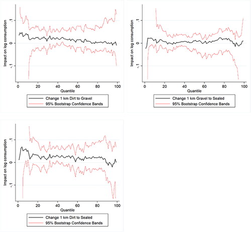
The effect of the difference between a kilometre of sealed and dirt road is on average relatively larger for the lowest 20 quantiles and relatively lower for the highest 20. The average effect on log consumption for the former is 0.041, while it is 0.007 for the latter. Similarly, the effect of the difference between gravel and dirt road is decreasing along the income distribution, with an average effect of 0.030 for the poorest 20 quantiles and 0.001 for the richest 20. However, the large confidence bands generated by the bootstrapping procedure mean that these trends are not statistically significant. We interpret the results from the GQR model as limited evidence that upgrading dirt roads disproportionately benefits the poorest households in PNG and may thus be regarded a pro-poor policy measure.

6. Conclusion

In this paper, we examine the effects of the quality of PNG’s road network on rural household welfare over a 13-year period. We find evidence that upgrading roads leads to improvements in household welfare, housing quality, and school enrolment. The effects on consumption and poverty are higher for disadvantaged and more remote households. This finding complements the argument by Gibson and Rozelle (2003) that due to the sparse road network and the remoteness of many poor households, infrastructure spending may be one of the few feasible targeted antipoverty measures in PNG. Our results also show that upgrading roads supports the structural transformation of households away from subsistence farming and toward market-oriented activities. This is consistent with the inhomogeneous impact on consumption and suggests that connecting rural households to local markets particularly benefits smallholder farmers.

Our identification strategy makes only use of existing administrative road inventory data in combination with repeated cross-sectional household surveys. These kinds of datasets are available for many other countries as well. The appeal of our method thus lies in its simplicity and its low data requirements. It easily lends itself for replication elsewhere, and again in PNG after the next national household survey has been conducted.

Acknowledgements

The authors wish to thank John Gibson for his assistance with the survey data and his useful comments during early phases of the research. In addition, we thank Bryant Allen for providing access to the PNGRIS database.

Disclosure statement

No potential conflict of interest was reported by the author(s).

Data availability statement

The authors commit to make the data and do-files available on request.

Additional information

Funding

This work was supported by the Asian Development Bank [Regional project 46185 ‘Developing Impact Evaluation Methodologies, Approaches, and Capacities in Selected Developing Member Countries’, subproject 2].

Notes

1 Since the PNGHS 96 used sampling based on census units from the census of 1990, on which data is unavailable, we first had to recode the 1990 census units. For this, we relied on the census unit names listed in Gibson and Rozelle (1998) as well as the generous help of staff at the National Statistical Office of PNG. The HIES 09/10 was sampled from the census of 2000, which made locating the census units straightforward.

2 The two road datasets offer slightly different spatial representations of common road segments, with positional differences ranging up to several hundred metres. To ensure that our analysis is not influenced by differences in the coverage and spatial representation of the road network across the two years, we use the representation of the 2009 map for both maps. That means that we have to include the information on surface type and road condition of 2000 in the 2009 road map. We match roads based on road section IDs, and where those are missing, on spatial proximity. It should also be mentioned that we cannot make use of the most detailed survey of the national road network to date, the Comprehensive Visual Road Condition Survey, which was collected in 2014 by the Papua New Guinea-Australia Transport Sector Support Program (TSSP) together with the DoW. Due to the sudden heavy rise in national road investments starting in 2011, we believe that the conditions in this new survey do not adequately reflect the conditions around the time the HIES 09/10 was conducted.

3 Details on the construction of this variable, as well as a discussion of remote sensing as an alternative to identify road quality and surface type, can be found in the appendix of Edmonds, Wiegand, Koomen, Pradhan, and Andrée (2018).

4 The latter criterion leads to the exclusion of three settlements that can only be reached by water. All towns with more than 1000 inhabitants in 2011 were already towns in 2000.

5 We construct per capita expenditure as well as regional poverty lines as explained in Gibson and Rozelle (1998) and Gibson (2012). Particularly, we use the revised consumption figures, poverty lines, and sampling weights for the PNGHS 96 explained in Gibson (2012) to make expenditure and poverty comparable between the two surveys. For the HIES 09/10, Gibson (2012) suggests three different consumption figures. Due to evidence of diary fatigue, we use the figure based on the shortest time horizon (7 days). The poverty lines we use take the cost of a locally consumed food basket and add the non-food spending of households whose food expenditures exactly meet this cost (Lanjouw & Lanjouw, 2001).

6 Like Gibson and Rozelle (2003), we assign children aged between 0 and 6 years a weight of 0.5, while children older than 6 years as well as adults are assigned a weight of 1.

7 The definitions vary slightly between survey rounds. For the PNGHS 96, the variable indicates that in the two weeks prior to the survey, at least one household member engaged in the production of sago, bananas, corn, sweet potato, cassava, taro, or other fresh fruits or vegetables without selling them. For the HIES 09/10, the variable indicates that in the week prior to the survey, at least one household member engaged in agricultural production for own consumption. The means of both variables are very close, as shown in Table 1.

8 Measures of housing quality were left out in the construction of the consumption figures (Gibson, 2012), so are not part of the first two outcome variables.

9 The sampling weights used in the regressions of consumption and poverty status are person-specific, those in the regressions of schooling are children-specific, and those in the other regression are household-specific.

10 We take the population size for 1996 from the 2000 census, and the population size for 2009/10 from the 2011 census.

References

- Adukia, A., Asher, S., & Novosad, P. (2020). Educational investment responses to economic opportunity: Evidence from Indian road construction. American Economic Journal: Applied Economics, 12(1), 348–376.
- Aggarwal, S. (2018). Do rural roads create pathways out of poverty? Evidence from India. Journal of Development Economics, 133, 375–395. doi:10.1016/j.jdeveco.2018.01.004
- Anderson, M. L. (2008). Multiple inference and gender differences in the effects of early intervention: A reevaluation of the abecedarian, perry preschool, and early training projects. Journal of the American Statistical Association, 103(484), 1481–1495. doi:10.1198/016214508000000841
- Asher, S., & Novosad, P. (2020). Rural roads and local economic development. American Economic Review, 110(3), 797–823. doi:10.1257/aer.20180268
- Banerjee, A., Duflo, E., & Qian, N. (2020). On the road: Access to transportation infrastructure and economic growth in China. Journal of Development Economics, 145, 102442–36. doi:10.1016/j.jdeveco.2020.102442
- Bell, C., & van Dillen, S. (2014). How does India’s rural roads program affect the grassroots? Findings from a survey in Orissa. Land Economics, 90(2), 372–394. doi:10.3368/le.90.2.372
- Binswanger, H. P., Khandker, S. R., & Rosenzweig, M. R. (1993). How infrastructure and financial institutions affect agricultural output and investment in India. Journal of Development Economics, 41(2), 337–366. doi:10.1016/0304-3878(93)90062-R
- Bryan, J., & Shearman, P. (2008). Papua New Guinea resource information system handbook (3rd ed.). Port Moresby, Papua New Guinea: University of Papua New Guinea.
- Burgess, R., Jedwab, R., Miguel, E., Morjaria, A., & Padró I Miquel, G. (2015). The value of democracy: Evidence from road building in Kenya. American Economic Review, 105(6), 1817–1851. doi:10.1257/aer.20131031
- Casaburi, L., Glennerster, R., & Suri, T. (2013). Rural roads and intermediated trade: Regression discontinuity evidence from Sierra Leone (Working Paper). Cambridge, MA: Harvard University Department of Economics Working Paper.
- Castaing Gachassin, M. (2013). Should I stay or should I go? The role of roads in migration decisions. Journal of African Economies, 22(5), 796–826. doi:10.1093/jae/ejt004
- Dercon, S., Gilligan, D. O., Hoddinott, J., & Woldehanna, T. (2009). The impact of agricultural extension and roads on poverty and consumption growth in fifteen Ethiopian villages. American Journal of Agricultural Economics, 91(4), 1007–1021. doi:10.1111/j.1467-8276.2009.01325.x
- Dercon, S., Hoddinott, J., & Woldehanna, T. (2012). Growth and chronic poverty: Evidence from rural communities in Ethiopia. Journal of Development Studies, 48(2), 238–253. doi:10.1080/00220388.2011.625410
- Dornan, M. (2016). The political economy of road management reform: Papua New Guinea’s national road fund. Asia & the Pacific Policy Studies, 3(3), 443–457. doi:10.1002/app5.142
- Edmonds, C., Wiegand, M., Koomen, E., Pradhan, M., & Andrée, B. P. J. (2018). Assessing the impact of road development on household welfare in rural Papua New Guinea. In N. Yoshino, M. Helble, & U. Abidhadjaev (Eds.), Financing infrastructure in Asia and the Pacific: Capturing impacts and new sources (pp. 189–235). Tokyo: Asian Development Bank Institute.
- Gertler, P. J., Gonzalez-Navarro, M., Gračner, T., & Rothenberg, A. D. (2022). Road maintenance and local economic development: Evidence from Indonesia’s highways (NBER Working Paper No. w30454). Cambridge, MA: National bureau of economic research (NBER).
- Gibson, J. (2012). Papua New Guinea poverty profile. Based on the household income and expenditure survey (Technical Report). Port Moresby, Papua New Guinea: Department of National Planning and Monitoring.
- Gibson, J., & Olivia, S. (2010). The effect of infrastructure access and quality on non-farm enterprises in rural Indonesia. World Development, 38(5), 717–726. doi:10.1016/j.worlddev.2009.11.010
- Gibson, J., & Rozelle, S. (1998). Results of the household survey component of the 1996 poverty assessment for papua new Guinea (Technical Report). Port Moresby, Papua New Guinea: Department of National Planning and Monitoring.
- Gibson, J., & Rozelle, S. (2003). Poverty and access to roads in Papua New Guinea. Economic Development and Cultural Change, 52(1), 159–185. doi:10.1086/380424
- Jusi, P., Mumu, R., Jarvenpaa, S., Neausemale, B., & Sangrador, E. Jr. (2003). Road asset management system implementation in Pacific region: Papua New Guinea. Transportation Research Record: Journal of the Transportation Research Board, 1819(1), 323–332. doi:10.3141/1819b-41
- Khandker, S. R., Bakht, Z., & Koolwal, G. B. (2009). The poverty impact of rural roads: Evidence from Bangladesh. Economic Development and Cultural Change, 57(4), 685–722. doi:10.1086/598765
- Khandker, S. R., & Koolwal, G. B. (2010). How infrastructure and financial institutions affect rural income and poverty: Evidence from Bangladesh. The Journal of Development Studies, 46(6), 1109–1137. doi:10.1080/00220380903108330
- Khandker, S. R., & Koolwal, G. B. (2011). Estimating the long-term impacts of rural roads: A dynamic panel approach (Policy Research Working Paper). Washington, DC: World Bank.
- Knox, J., Daccache, A., & Hess, T. (2013). What is the impact of infrastructural investments in roads, electricity and irrigation on agricultural productivity? CEE review 11-007. Collaboration for Environmental Evidence (CEE) Syntheses. http://www.environmentalevidence.org/wp-content/uploads/2014/05/CEE11-007.pdf (last accessed 6 December 2016).
- Kwa, E., Howes, S., & Lin, S. (2010). Review of the PNG–Australia Development Cooperation Treaty (1999). Canberra: Department of Foreign Affairs and Trade, Australian Government.
- Lanjouw, J. O., & Lanjouw, P. (2001). How to compare apples and oranges: Poverty measurement based on different definitions of consumption. Review of Income and Wealth, 47(1), 25–42. doi:10.1111/1475-4991.00002
- Lokshin, M., & Yemtsov, R. (2005). Has rural infrastructure rehabilitation in georgia helped the poor? The World Bank Economic Review, 19(2), 311–333. doi:10.1093/wber/lhi007
- Lucius, D. (2010). Civil works capacity constraints (Technical Report). Manila: Asian Development Bank.
- Mu, R., & van de Walle, D. (2011). Rural roads and local market development in Vietnam. Journal of Development Studies, 47(5), 709–734. doi:10.1080/00220381003599436
- Mundlak, Y. (1978). On the pooling of time series and cross section data. Econometrica, 46(1), 69–85. doi:10.2307/1913646
- Nguyen, C. V. (2019). Impacts of rural roads on household welfare in Vietnam: Evidence from a replication study. Journal of Economics and Development, 21(1), 83–112.
- Powell, D. (2020). Quantile treatment effects in the presence of covariates. The Review of Economics and Statistics, 102(5), 994–1005. doi:10.1162/rest_a_00858
- Shrestha, S. A. (2020). Roads, participation in markets, and benefits to agricultural households: Evidence from the topography-based highway network in Nepal. Economic Development and Cultural Change, 68(3), 839–864. doi:10.1086/702226
- Stead, D. (1990). Engineering geology in Papua New Guinea: A review. Engineering Geology, 29(1), 1–29. doi:10.1016/0013-7952(90)90079-G
- World Food Programme and Logistics Cluster. (2011). Papua New Guinea emergency preparedness: Operational logistics contingency plan part 2 – existing response capacity and overview of logistics situation (Technical Report). Rome, Italy: World Food Programme (WFP). http://reliefweb.int/sites/reliefweb.int/files/resources/PNG%20Logistics%20CP%20-%20Part%202%20-%20Existing%20Response%20Capacity%20and%20Logistics%20Overview.pdf (last accessed 21 December 2016)