Teaching the COVID-19 lockdown using the Keynesian Cross

Abstract

I present a framework to teach the macroeconomic effects of COVID-19 using the Keynesian Cross. I show that the rest of the economy suffers from a decline in demand once one sector of the economy is shut down and that the government spending and tax multipliers are smaller than usual. Fully insuring workers in the sector that is shut down cannot prevent a recession, but for the same aggregate transfers, such targeted income transfers do more to restore aggregate output than unconditional transfers. An extension to the $IS$ curve shows that a lockdown results in deflation. These insights can be taught in an introductory or intermediate macroeconomics course.

Keywords:

• Keynesian Cross
• lockdown
• multiplier
• supply shock
• transfers

View correction statement:

Correction

In the United States, the lockdown in response to the COVID-19 pandemic increased the unemployment rate to its highest level since the Great Depression (BLS 2020). For current undergraduate students of macroeconomics, this lockdown is the biggest macroeconomic event in their (admittedly short) adult lives. I propose a framework that is simple but introduces students to research-frontier macroeconomic thinking about this episode, using a graphical apparatus that students already know. This simple framework highlights the large heterogeneity between workers in different sectors and can explain the peculiar behavior of prices and savings rates that are characteristic of the COVID-19 lockdown. It also addresses the effectiveness of the economic policies conducted by governments to fight the recession alongside the pandemic. Finally, it captures the emerging consensus that changes in both demand and supply contributed to the current contraction of economic activity.

This article follows the literature in modeling a lockdown as a supply shock; a lockdown imposes a reduction in aggregate supply by shutting down one or more sectors of the economy that are contact-intensive and provide nonessential goods or services. However, if a negative supply shock were the full story, how can instructors explain to their students why the price level fell? Figure 1 presents the PCE price index for the United States between January 2000 and May 2020.¹ The figure shows that at the height of the lockdown in April 2020, consumer prices fell by 0.5%. Although a deflation of 0.5% is hardly spectacular, it is remarkable that such a deflation occurs during a major negative supply shock.

Figure 1. Percent price changes from preceding month for Personal Consumption Expenditures (PCE), United States, January 2000–May 2020.

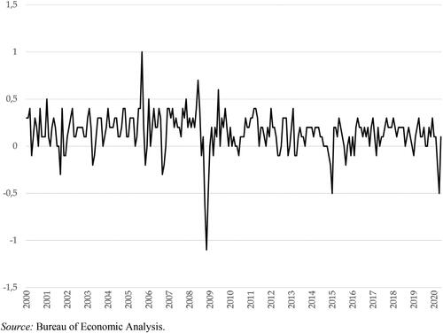
I explain how deflation can result from a negative supply shock by splitting a model economy into two sectors. In a lockdown, sector 1 will be shut down because it is contact-intensive and nonessential (e.g., restaurants). Sector 2 will not be shut down, either because it is not contact-intensive or because it is essential (e.g., healthcare or food supply). The size of sector 1 before the lockdown determines the size of the supply shock and also the fraction of pre-lockdown income that can no longer be spent in sector 1. Because workers in sector 1 no longer earn any income, they cannot spend on sector 2, either. As a result, demand in sector 2 declines as well, and prices fall. Only if transfers ensure workers in sector 1 of their pre-lockdown income can this additional demand response be circumvented, and the fall in output can be contained to the size of sector 1.

A two-sector Keynesian Cross captures this intuition. Introducing two sectors shows how spending in sector 2 partly depends on income earned in sector 1, and thus why prices in sector 2 fall when sector 1 is shut down. Moreover, distinguishing spending between two sectors, one of which is shut down, provides an intuition for a decrease in the marginal propensity to consume and can explain smaller tax and government spending multipliers. Whereas a standard one-sector Keynesian Cross could feature an exogenous decrease in the marginal propensity to consume, it would fail to show how spending in sector 2 depends on income earned in the sector that is shut down. Exactly this heterogeneity between sectors is fundamental to the COVID-19 lockdown in general and to the explanation of the observed deflation in particular.

A decrease in the average marginal propensity to consume is consistent with the evidence on savings during the lockdown, as shown in figure 2. This figure presents an unprecedented increase in the average savings rate in April 2020, showing that there is an important story on the demand side of a lockdown economy that cannot be captured by a decrease in autonomous spending in a one-sector Keynesian Cross such as modeled in The CORE Team (2021). At the same time, the fact that, despite such huge savings rates, deflation was only mild shows that a lockdown is not just a drop in demand, but that supply played a significant role too.

Figure 2. Personal savings as a percentage of personal disposable income. Monthly, United States, January 2000–May 2020.

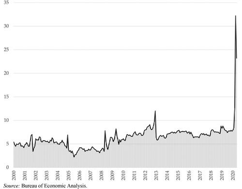
However, an average savings rate of over 30 percent suggests that the average American had no trouble making ends meet and provides little rationale for the extensive income support resorted to by the U.S. government and many other countries.² To understand the need for transfer policies and the macroeconomic importance of targeting them to workers in the sector that is shut down, I introduce a concave aggregate consumption function. This aggregate consumption function consists of two linear segments and thus features two different marginal propensities to consume: one at 1 and another at a lower level. Consequently, it allows workers in sector 1 to be liquidity-constrained, spending all income that they receive, while simultaneously, workers in sector 2 may save a large fraction of their income because they cannot spend on sector 1. As a result, the average savings rate may be high, consistent with figure 2, even though some workers are severely constrained in their consumption. The COVID-19 lockdown provides a particularly intuitive example to introduce students to such heterogeneity in marginal propensities to consume, the importance of which goes beyond the COVID-19 lockdown itself, for instance, because it can explain why multipliers are larger during recessions than booms (outside of lockdowns).³

Related literature

The main contribution of this article is that it provides a simple framework that introduces students to the research frontier on the most recent macroeconomic crisis. This framework is inspired by Guerrieri et al. (2020), who introduce a small-scale DSGE model with two sectors and show that a lockdown can result in what they call “Keynesian supply shocks”: supply shocks that cause a change in demand that exceeds the size of the shock. Supply shocks are more likely to be “Keynesian” under incomplete markets and when the intertemporal elasticity of substitution is sufficiently high and the elasticity of substitution across sectors is not too large. Guerrieri et al. also show that using transfers to provide full insurance to workers in the shutdown sector is optimal, despite a smaller multiplier of fiscal policy.

I obtain Keynesian supply shocks and similar conclusions about the effectiveness of fiscal policy using models and a graphical apparatus that are already familiar to undergraduate students: a Keynesian aggregate consumption function without intertemporal optimization or micro-foundations. The aggregate consumption function pins down the marginal propensities to consume in each sector. Because the marginal propensity to consume for workers in sector 2 falls when they cannot spend on sector 1, multipliers are small since the effect of every subsequent spending round is smaller. The large marginal propensity to consume for workers in sector 1, which explains why transfers should target them, results from the introduction of a concave consumption function. This concave consumption function provides a highly simplified representation of the findings of decades of research on consumption decisions (Carroll 2001) and can be considered a secondary contribution.

Moreover, to explain deflation, the article goes beyond the results in Guerrieri et al. (2020) and extends the two-sector Keynesian Cross to the $IS$ curve and the $AS$-$AD$ model. This extension shows that the $IS$ and $AD$ curves shift leftwards and become steeper. The leftward shift of the $IS$ curve beyond the size of the supply shock follows immediately from the results obtained in the Keynesian Cross. Combined with a horizontal $MP$ curve, this finding carries over to the $AD$ curve and results in deflation. The steeper $IS$ and $AD$ curves also imply that monetary policy is less powerful during a lockdown, even away from the zero lower bound.

These findings are consistent with other recent research on the impact of COVID-19, the effect of supply shocks on demand more generally, and the effectiveness of fiscal policy during lockdowns. Using a model with multiple sectors and downward nominal wage rigidities, Baqaee and Farhi (2020) show that negative shocks to factor supply can result in Keynesian unemployment, reducing both output and the price level. Challe (2020), in a contribution that predates COVID-19, combines incomplete markets and nominal rigidities to show that negative supply shocks can be deflationary. Auray and Eyquem (2020) apply that model to study the macroeconomic effects of a lockdown of one sector of the economy. Also using a Heterogeneous Agent New Keynesian model, Bayer et al. (2020) find that the multiplier of transfers conditional on unemployment substantially exceeds the multiplier of unconditional transfers. Faria e Castro (2020) and Bigio, Zhang, and Zilberman (2020) model the pandemic as a shock to the utility of contact-intensive services but similarly find that transfers (or credit policies) that target workers in the shutdown sector are the most effective in stabilizing income.⁴ Using a two-sector version of the textbook Keynesian Cross, the current model captures the essence of these contributions and is simple enough to teach to undergraduate students.

The model environment

The Keynesian Cross

To convey the intuition behind the concave consumption function, I first present a one-sector Keynesian Cross and its notation. I focus on the closed-economy version for simplicity.

Aggregate spending sums consumption $C,$ investment $I$, and government expenditure $G.$ Government expenditure $G$ consists of government purchases of goods and services but excludes transfers. At the aggregate level, some of the taxes collected by the government are redistributed as transfers. Aggregate taxes net of transfers are denoted by $T$.⁵ Because all spending ends up as someone’s income, aggregate income $Y$ is the sum of the spending categories: $Y=C+I+G$.

The textbook Keynesian Cross distinguishes aggregate or planned expenditure $PE$ from actual expenditure $Y$, in which unplanned investment makes up for the difference. Planned expenditure consists of aggregate consumption, planned investment, and government spending: $PE=C+I^p+G$. I focus on equilibria so that $Y=PE$ and all investment is planned. Investment and government spending are exogenous. It deviates from the textbook model by assuming that aggregate consumption is a function of disposable income $Y-T>0$ according to a piece-wise linear aggregate consumption function $$C=\{\begin{array}{c}Y-T, \mathit{\text{if Y}}-T \le \overline{C};\\ \overline{C}+c(Y-T- \overline{C}), \mathit{\text{if Y}}-T > \overline{C}.\end{array}$$

According to this function, consumers spend their full disposable income when disposable income is low. As soon as their disposable income hits a particular threshold, $\bar{C}\ge 0$, they start saving a fraction of their additional income, and their marginal propensity to consume falls from 1 to $c\in \left(0,1\right)$. Such a concave consumption function can be explained by liquidity constraints. In this interpretation, $\bar{C}$ denotes the level of disposable income at which liquidity constraints are no longer binding. For disposable income below $\bar{C}$ consumers may desire to consume more than their disposable income (e.g., because their marginal utility is high), but they are constrained by their available disposable income and their inability to borrow. In a lockdown, if an entire sector shuts down and workers lose their jobs and their incomes, one expects them to have trouble making ends meet and to use all available income from, e.g., transfers to pay for necessities. A concave consumption function can describe such behavior.⁶ Besides, it can explain why, outside of lockdowns, multipliers are larger in recessions than in booms. Finally, a standard consumption function with autonomous consumption raises the question of how autonomous consumption is paid for if income is close to zero. A concave consumption function avoids this question because consumption is constrained by disposable income.

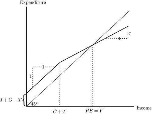
Aggregate expenditure is thus given by $PE=\min \left(\bar{C},Y-T\right)+c\max \left(Y-T-\bar{C},0\right)+I+G.$ Figure 3 presents the resulting Keynesian Cross, where the intercept of planned expenditure is given by $I+G-T,$ and any additional expenditure comes from aggregate consumption. Consumption increases one-for-one with disposable income until liquidity constraints are no longer binding, after which workers start saving, and only a fraction, $c<1$, of any additional disposable income is spent. Equilibrium income is given by the intersection of planned expenditure and the ${45}^{\circ }$ line.

Figure 3. The Keynesian Cross with a concave consumption function.

Two sectors

Now suppose the economy consists of two sectors: sector 1 and sector 2. In a lockdown, sector 1 will be shut down because it is contact-intensive and nonessential. Sector 2 will not be shut down. Denote the fraction of the population that is employed in sector 1 before the lockdown by $\varphi$. The remaining fraction, $1-\varphi$, is employed in sector 2. When the government imposes a lockdown, the supply of goods and services produced in sector 1 stops. To characterize the size of this supply shock, consider a simple supply side to the model.

Assumption 1.

The sectors’ production functions are identical and linear, with labor as the only input.

This assumption allows the same symbol, $\varphi$, for the fraction of workers that were employed in sector 1 to be used for the fraction of output supplied by sector 1. Assumption 1 thus simply implies $Y_1=\varphi Y$ and $Y_2=\left(1-\varphi \right)Y$.

On the demand side of this economy, denote aggregate consumption, investment, and government expenditure in each sector by $C_i$, $I_i$, and $G_i$ with $i\in \{1,2\}$. Of course, income earned in each sector follows from spending in the same sector, so that $Y_1=C_1+I_1+G_1$ and $Y_2=C_2+I_2+G_2$. Aggregate income consists of income in each sector: $Y=Y_1+Y_2$. For aggregate consumption, it is useful to distinguish between spending in a particular sector as defined above and spending by workers employed in a particular sector. Denote consumption by workers employed in sector $i\in \{1,2\}$ by ${\tilde{C}}_i$. Net taxes paid (or net transfers received) by workers employed in each sector are simply denoted by $T_i$.

Workers working in one sector have no different preferences than workers in the other sector but may have different disposable incomes. Assume that workers in both sectors always have non-negative disposable income, $Y_i\ge T_i$ for both $i\in \{1,2\}$, and that liquidity constraints stop to bind at the same level of disposable income for every worker. Decomposing the level of aggregate disposable income at which liquidity constraints are no longer binding, $\bar{C}$, between workers employed in each sector (of which a fraction, $\varphi$, work in sector 1 and a fraction, $1-\varphi$, work in sector 2), consumption by workers employed in sector 1 is given by ${\tilde{C}}_1=\min \left(\varphi \bar{C},Y_1-T_1\right)+c\max \left(Y_1-T_1-\varphi \bar{C},0\right)$ and analogously for ${\tilde{C}}_2$.

Assume that all consumption up to the point where liquidity constraints are no longer binding is spent in sector 2.⁷ Any additional disposable income will be spent in each sector according to sectoral marginal propensities to consume: $c_i$ for $i\in \{1,2\}$ with $c_1+c_2\equiv c<1$. The marginal propensities to consume in each sector are the same for all workers. Consumption in sector 2 is thus given by (1) $$\begin{array}{cc}{C}_2& =\min \left(\varphi \bar{C},Y_1-T_1\right)+c_2\max \left(Y_1-T_1-\varphi \bar{C},0\right)\\ & +\mathrm{ }\min \left(\left(1-\varphi \right)\bar{C},Y_2-T_2\right)+c_2\max \left(Y_2-T_2-\left(1-\varphi \right)\bar{C},0\right)\ge 0,\mathrm{ }\end{array}$$(1) and consumption in sector 1 is simply (2) $$C_1=c_1\max \left(Y_1-T_1-\varphi \bar{C},0\right)+c_1\max \left(Y_2-T_2-\left(1-\varphi \right)\bar{C},0\right)\ge 0.$$(2)

To rule out indeterminacy, make the following assumption on the exogenous variables:⁸

Assumption 2.

Before a lockdown, $I_1+G_1-T_1>\varphi \bar{C}$ and $I_2+G_2-T_2>\left(1-\varphi \right)\bar{C}$.

This assumption is a sufficient condition to ensure that no worker is liquidity-constrained before a lockdown, as stated in the following lemma.

Lemma 1.

Suppose assumption 2 holds. Then, disposable income in each sector is such that there are private savings in each sector: $Y_1-T_1>\varphi \bar{C}$ and $Y_2-T_2>\left(1-\varphi \right)\bar{C}$.

Proof.

Imposing assumption 2 on the accounting identity for $Y_1$ shows that, $$\begin{array}{cc}{Y}_1\equiv C_1+I_1+G_1& >C_1-T_1+\varphi \bar{C}\\ Y_1-T_1& >\varphi \bar{C},\end{array}$$ since $C_1\ge 0$ from (2). The proof for $Y_2-T_2>\left(1-\varphi \right)\bar{C}$ is analogous.

In graphical terms, assumption 2 thus ensures that planned expenditure in figure 3 crosses the ${45}^{\circ }$ line from above. Assumption 2 is stated in terms of exogenous variables, but for didactic purposes, one also may make assumptions on the endogenous variables in lemma 1 and directly assume that before the lockdown $Y_1-T_1>\varphi \bar{C}$ and $Y_2-T_2>\left(1-\varphi \right)\bar{C}$.

Finally, some results require a certain proportionality in the components of GDP across the two sectors. Assume thus the following:

Assumption 3.

Before a lockdown,

1. workers in both sectors pay equal per capita taxes, in particular $T_2=\left(1-\varphi \right)T$;

2. exogenous expenditure is proportional across sectors: $\left(1-\varphi \right)\left(I+G\right)=I_2+G_2$.

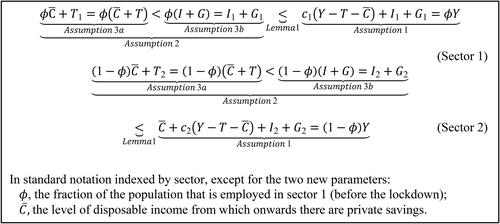
The full set of assumptions is summarized in figure 4. Only assumption 2 is required for all results. Two inequalities are not assumed but are the content of lemma 1 and are indicated as such.⁹

Figure 4. Summary of assumptions about the model environment before the lockdown.

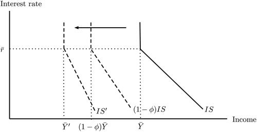
The supply shock

Now consider the economic shock that follows from a lockdown on sector 1. Variable names (like $Y$) will denote pre-lockdown or unchanged values, and variable names with prime (like $Y\prime$) will denote values during a lockdown. Suppose that before the lockdown, the economy is in equilibrium, such that $Y=Y_1+Y_2$ represents equilibrium or long-run aggregate supply (LRAS). Figure 5a shows this $\mathit{LRAS}$ line, together with an upward-sloping $AS$ curve and a downward-sloping $AD$ curve that cross potential output at $A$ (pinned down by price expectations).

Figure 5. AS-AD diagram with a shock to supply, and a resulting decline in demand.

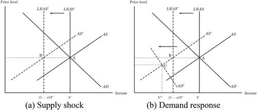
During the lockdown, the economy simply cannot supply the goods and services produced in sector 1 anymore. Without reallocation of workers across sectors, supply thus drops to $Y_2$ which equals $\left(1-\varphi \right)Y$ by assumption 1. Because supply in sector 1 is zero at any price level, the lockdown should be understood as a shift of potential output. In figure 5a, a lockdown thus is described as a shift of long-run aggregate supply to $\mathit{LRAS}\prime$ at $\left(1-\varphi \right)Y$. Assuming a lack of perfect foresight, the short-run aggregate supply curve during the lockdown $AS\prime$ follows the long-run aggregate supply curve. Deviations from the expected price level can change short-run supply along the curve because higher prices can boost labor demand in sector 2, attracting more workers to that sector, while lower prices decrease supply in sector 2.¹⁰

The question now is what will happen to the $AD$ curve. Will it shift to B, or to the left or right of it? An application of the two-sector Keynesian Cross shows that aggregate demand endogenously amplifies the shock to aggregate supply so that the $AD\prime$ curve shifts leftwards even more than the $AS$ curve. Figure 5b presents this decline in demand intersecting supply at $C$, the output level $Y\prime$ that is smaller than $\left(1-\varphi \right)Y$ and the resulting deflation.

The Keynesian Cross in a lockdown

In any lockdown equilibrium, all spending on sector 1 stops: $C{\prime }_1=I_1\prime =G_1\prime =0$. As a result, income earned in sector 1 in the lockdown-economy $Y_1\prime$ is zero, and aggregate income of the lockdown economy is equal to income earned in sector 2: $Y\prime =Y{\prime }_2$. This section of the article shows what will happen to income earned in sector 2.

To make sure that workers in sector 1 have non-negative disposable income, assume that the government immediately agrees to a tax holiday for workers in sector 1 but does not give any net transfers (yet): $T_1\prime =0$. As a result, workers in sector 1 will purchase nothing from sector 2. Investment, government expenditure, and net taxes in sector 2 remain unchanged: $I_2\prime =I_2$, $G_2\prime =G_2$, and $T{\prime }_2=T_2$. Also, assume that the level of disposable income at which liquidity constraints are no longer binding, $\bar{C}$, and the marginal propensity to consume in sector 2, $c_2$, remain the same. The next proposition shows the existence of Keynesian supply shocks in this environment.

Proposition 1

(Keynesian supply shocks). Suppose assumption 2 holds. Then, income earned in sector 2 during a lockdown is strictly smaller than income in sector 2 before the lockdown:$$Y_2\prime <Y_2$$

Proof.

From lemma 1, it follows that before the lockdown, income in sector 2 equals (3) $$\begin{array}{cc}{Y}_2& =\bar{C}+c_2\left(Y_1+Y_2-T_1-T_2-\bar{C}\right)+I_2+G_2\hspace{0.33em}\hspace{0.33em}\iff \\ & =\bar{C}+\frac{c_2}{1-c_2}\left(Y_1-T_1-T_2\right)+\frac{1}{1-c_2}\left(I_2+G_2\right).\end{array}$$(3)

In a lockdown, $Y_1\prime =0$. As a result, consumption by workers (that used to be) employed in sector 1 falls to zero: $\tilde{C}{\prime }_1=0$. So the lockdown does not only stop consumption in sector 1 but also consumption by workers employed in sector 1. Consequently, (4) $$Y_2\prime =\min \left(\left(1-\varphi \right)\bar{C},Y_2\prime -T_2\right)+c_2\max \left(Y_2\prime -T_2-\left(1-\varphi \right)\bar{C},0\right)+I_2+G_2.$$(4)

Assumption 2 implies that workers in sector 2 are still not liquidity-constrained, so that (5) $$\begin{array}{cc}{Y}_2\prime & =\left(1-\varphi \right)\bar{C}+c_2\left(Y_2\prime -T_2-\left(1-\varphi \right)\bar{C}\right)+I_2+G_2\hspace{0.33em}\hspace{0.33em}\iff \\ & =\left(1-\varphi \right)\bar{C}-\frac{c_2}{1-c_2}{T}_2+\frac{1}{1-c_2}\left(I_2+G_2\right),\end{array}$$(5) which is clearly less than $Y_2$. Note that the difference comes both from binding liquidity constraints ($\varphi \bar{C}$) and from missing additional consumption from the marginal propensity to consume additional disposable income earned in sector 1 ($Y_1-T_1-\varphi \bar{C}$).

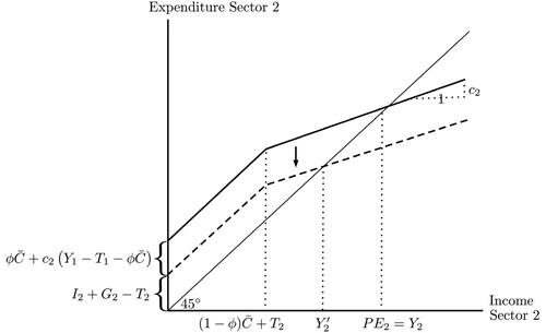
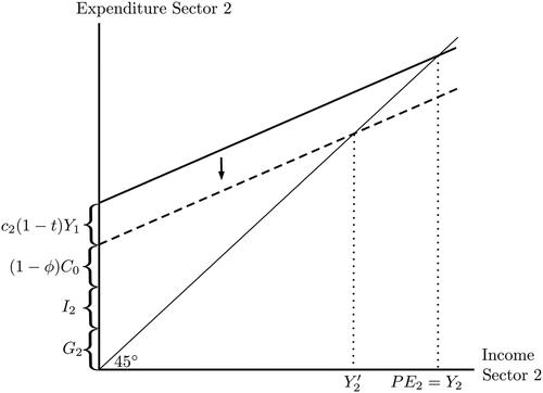
Before the lockdown, workers in both sectors spend in both sectors. In a lockdown, no one can spend in sector 1, but workers (that used to be) employed in sector 1 cannot spend in sector 2, either, because they have no income. As a result, income in sector 2 decreases as well. This intuition can be shown in the Keynesian Cross if it is restricted to expenditure and income in sector 2. Figure 6 shows what happens to income in sector 2 whenever spending from sector 1 disappears.¹¹ A reduction in exogenous spending reduces income in sector 2, which is exacerbated by reduced spending by workers in sector 2 as the result of a lower income. This multiplier process settles at $Y{\prime }_2$. This model exactly captures the intuition behind Keynesian supply shocks in Guerrieri et al. (2020).¹²

Figure 6. The Keynesian Cross of sector 2 in which expenditure from sector 1 workers in sector 2 is treated as exogenous.

Another way to understand the result of Keynesian supply shocks, inspired by Rowe (2020), is to realize that shutting down only one sector that employs a fraction, $\varphi$, of the workers and which constitutes a fraction, $\varphi$, of national income by assumption 1 is not the same as shutting down both sectors for that same fraction, $\varphi$. In other words, the economy shrinks by more than the size of sector 1. The following proposition shows the payoff of introducing two sectors in the Keynesian Cross for the analysis of the aggregate economy.

Proposition 2

(A proportional lockdown). Suppose assumptions 2 and 3 hold and consider the case in which both sectors are shut down for a fraction, $\varphi$, of the original level of aggregate income, and a fraction, $\varphi$, of taxes is given a tax holiday. Aggregate income in this case is strictly larger than aggregate income in the lockdown economy: $\left(1-\varphi \right)Y>Y\prime$.

Proof.

From lemma 1, it follows that aggregate income before the lockdown is (6) $$\begin{array}{cc}Y& =\bar{C}+c\left(Y-T-\bar{C}\right)+I+G\hspace{0.33em}\hspace{0.33em}\iff \\ & =\bar{C}-\frac{c}{1-c}T+\frac{1}{1-c}\left(I+G\right),\end{array}$$(6) so that a representation for $\left(1-\varphi \right)Y$ is (7) $$\begin{array}{cc}\left(1-\varphi \right)Y& =\left(1-\varphi \right)\bar{C}-\frac{c}{1-c}\left(1-\varphi \right)T+\frac{1}{1-c}\left(1-\varphi \right)\left(I+G\right),\\ & =\left(1-\varphi \right)\bar{C}-\frac{c}{1-c}{T}_2+\frac{1}{1-c}\left(I_2+G_2\right),\end{array}$$(7) by assumptions 3a and 3b. It follows that $\left(1-\varphi \right)Y$ from (7) exceeds $Y\prime$ from (5) because $$\begin{array}{cc}\frac{I_2+G_2}{1-c}-c\frac{T_2}{1-c}& >\frac{I_2+G_2}{1-c_2}-c_2\frac{T_2}{1-c_2},\hspace{0.33em}\hspace{0.33em}\iff \\ \left(I_2+G_2-c{T}_2\right)\left(1-c_2\right)& >\left(I_2+G_2-c_2{T}_2\right)\left(1-c\right),\hspace{0.33em}\hspace{0.33em}\iff \\ -c_2\left(I_2+G_2\right)-c{T}_2& >-c\left(I_2+G_2\right)-c_2{T}_2,\hspace{0.33em}\hspace{0.33em}\iff \\ c_1\left(I_2+G_2\right)& >c_1{T}_2,\end{array}$$ since $c_1+c_2\equiv c$, and $I_2+G_2>T_2$ by assumption 2.

The proof shows that the effects of a lockdown are larger than proportional precisely because people cannot consume in sector 1 during a sectoral lockdown. Assumption 2 implies that the smaller propensity to consume earned income during a lockdown dominates the contractionary effect of taxes (which is also smaller during a lockdown). Assumption 3a ensures an equal reduction in aggregate taxes in the two scenarios. The role of assumption 3b is simply to guarantee that the reduction of consumption in sector 1 is not compensated by disproportionate exogenous spending in sector 2.¹³

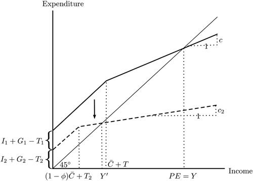
Figure 7 summarizes the effects discussed so far. It shows how pre-lockdown income $Y$ falls to income $Y\prime$ during the lockdown for three reasons. First, exogenous spending in sector 1 disappears $I{\prime }_1+G{\prime }_1-T{\prime }_1=0$ and the intercept of planned expenditure falls. Second, workers in sector 1 become liquidity-constrained and cannot even buy necessities, and the kink in the consumption function moves left to $\left(1-\varphi \right)\bar{C}+T_2$. Third, workers in sector 2 can no longer spend in sector 1, and the slope of the flat part of the expenditure function falls from $c$ to $c_2$. This reduction of the slope of the expenditure function is consistent with the evidence in figure 2. It captures the finding that workers in sector 2 start saving more because they cannot go on holiday or to restaurants or concerts. The next section shows that this extra saving is also crucial to understanding the effectiveness of fiscal policy in a lockdown.

Figure 7. The two-sector Keynesian Cross and the result of a lockdown.

Fiscal policy in a lockdown

This section analyzes the size of the multiplier of government expenditure in sector 2, and the effects of taxes and transfers. Because of the concave consumption function, it is then important to distinguish between transfers to workers (that used to be) employed in sector 1 and workers in sector 2. As before, assume that workers in sector 1 have non-negative disposable income during a lockdown, i.e., do not pay taxes.

Proposition 3.

Suppose assumption 2 holds. Then, the government spending and tax multipliers are smaller (in absolute terms) during a lockdown than before.

Proof.

Taking first differences of (5) yields (8) $$\Delta Y\prime =\frac{-c_2}{1-c_2}\Delta T_2+\frac{1}{1-c_2}\left(\Delta I_2+\Delta G_2\right).$$(8)

The government spending multiplier (provided that all such expenditure is in sector 2) is equal to $1/\left(1-c_2\right)$. Compared to the usual multiplier of $1/\left(1-c\right)$ (that can be similarly derived by taking first differences of (6)), the multiplier is smaller since $c_2<c$. Similarly, the tax multiplier is $-c_2/\left(1-c_2\right)$ instead of $-c/\left(1-c\right)$.

The government spending multiplier is smaller, precisely because in every “round,” a smaller fraction of the additional income is spent than whenever additional income also can be spent in sector 1, and because spending thus never ends up in the hands of workers in sector 1 who would consume their full income. Similarly, the tax multiplier is less negative, such that increasing taxes on workers in sector 2 is not as contractionary as usual. A drop in autonomous spending in a one-sector Keynesian Cross, such as presented in The CORE Team (2021), cannot explain smaller multipliers.

Whereas giving transfers to workers in sector 2 is thus not very expansionary because of the concave consumption function, the same does not equally apply to transfers to workers (that used to be) employed in sector 1. Indeed, because workers in sector 1 are liquidity-constrained during a lockdown, they will spend any additional income one-for-one on additional consumption until $-T_1\prime =\varphi \bar{C}$. Up to this point, their transfer payments multiplier thus equals the government expenditure multiplier. The following corollary summarizes these results.

Corollary 1.

During a lockdown, the marginal multiplier on transfers to sector 1 workers,

1. is equal to the government spending multiplier for $-T_1\prime <\varphi \bar{C}$: $1/\left(1-c_2\right)$;

2. is equal to the multiplier on transfers to workers in sector 2 for $-T_1\prime \ge \varphi \bar{C}$: $c_2/\left(1-c_2\right)$.

On the one hand, although the multiplier on transfer payments to workers in sector 1 is equal to the government spending multiplier, it follows from proposition 3 that this multiplier is still smaller than the government spending multiplier before a lockdown. Moreover, if the transfers make the liquidity constraints no longer binding or if the transfers can be claimed by workers employed in sector 2, the multiplier is equal to the (negative of the) tax multiplier, and thus even smaller than the government spending multiplier during a lockdown. Precisely because the tax multiplier is less negative, net tax decreases or transfers to workers in sector 2 do not deliver as much additional consumption as before the lockdown. Whereas workers in sector 1 have a marginal propensity to consume of 1 until they are no longer liquidity-constrained, workers in sector 2 have only a propensity of $c_2<c<1$, because they cannot spend in sector 1. From the perspective of stabilizing output, a lockdown is therefore a relatively bad time to introduce a universal basic income. These results are broadly consistent with the findings in Bayer et al. (2020) and Chetty et al. (2020).

On the other hand, transfers targeted to workers in sector 1 may be one of the most effective policies to fight Keynesian supply shocks. Precisely because the multiplier on transfer payments to workers in sector 1 is equal to the government spending multiplier up to the level where liquidity constraints are no longer binding, targeted transfers are as expansionary as government spending while providing insurance to workers in sector 1. By giving (debt-financed) transfers to workers in sector 1 equal to their previous disposable income $Y_1-T_1$, income in sector 2 can be restored to its pre-lockdown level, enabling all workers in sector 2 to remain employed because the economy returns to the situation in (3). The intuition for this result also can be seen in figure 6: with transfers equal to $Y_1-T_1$, workers in sector 1 spend $\varphi \bar{C}+c_2\left(Y_1-T_1-\varphi \bar{C}\right)$ in sector 2, and the economy moves from $Y{\prime }_2$ to $Y_2$. From the level where liquidity constraints would no longer be binding onwards, government spending would be a cheaper policy to make $Y{\prime }_2$ unaffected, but it would not provide insurance.

Aggregate demand and monetary policy

To be able to analyze the effect of a lockdown on the price level and on the effectiveness of monetary policy, this section extends the analysis to the $IS$ curve and the $AS$-$AD$ model. First, assume that investment in each sector is a negative function of the real interest rate: $I_1=I_1\left(r\right)$ and $I_2=I_2\left(r\right)$. As before, during a lockdown, investment in sector 1 is shut down and $I_1\left(r\right)=0$.¹⁴ Because substituting $I_2\left(r\right)$ in (3) and (5) in no way affects the proof of proposition 1, the next corollary follows.

Corollary 2.

(Keynesian supply shocks with investment). For the same interest rate $r$, income in sector 2 during a lockdown is strictly smaller than income in sector 2 before the lockdown: $Y_2\prime \left(r\right)<Y_2\left(r\right)$.

The result that Keynesian supply shocks are robust to the introduction of an investment function does not immediately imply that the $IS$ curve moves left. However, because in a lockdown, only $I_2$ can respond to the interest rate, one can expect that the decrease in investment as the result of the same increase in the interest rate is smaller in the lockdown economy than before the lockdown. As the result of this reduced sensitivity to the interest rate, and because of the smaller marginal propensity to consume since workers in sector 2 can no longer spend in sector 1 (as can be seen in the multiplier on investment in (8)), the $IS$ curve will be steeper. To guarantee that the result of proposition 2 carries over to the $IS$ curve, assume that investment in sector 1 and investment in sector 2 respond to the interest rate in proportion to the relative size of their respective sectors:

Assumption 4.

Before a lockdown, investment in each sector $i\in \{1,2\}$ is given by $I_i=\max \left({\bar{I}}_i-b_{i}r,0\right)$, in which

1. $b_i>0$ captures the responsiveness of investment to the interest rate in each sector, with $\left(1-\varphi \right)b_1=\varphi b_2$

2. ${\bar{I}}_i$ denotes autonomous investment in each sector, with $\left(1-\varphi \right){\bar{I}}_1=\varphi {\bar{I}}_2$.

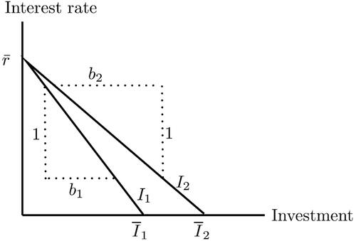
Given that the investment functions feature a kink, it is useful to define the interest rate $r$ at which investment becomes zero, as below:

Lemma 2.

There exists one $\bar{r}$, such that for $r<\bar{r}$, $I_i>\mathrm{0, and for }\mathrm{r\ge }\stackrel{\mathrm{‾}}{r}\mathrm{, }{I}_i=\mathrm{0, in each sector }i\in \left\{\mathrm{1,2}\right\}$.

Proof.

Note that ${\bar{I}}_1/b_1={\bar{I}}_2/b_2$ by assumptions 4a and 4b, which defines $\bar{r}$.

This finding is presented graphically in figure 8, which shows that the proportionality assumed in assumption 4 implies that $I_1$ and $I_2$ both go through $\left(0,\bar{r}\right)$. The following proposition then formalizes that the $IS$ curve moves left by more than a fraction, $\varphi$, and becomes steeper in a lockdown.

Figure 8. Investment in sector 1 and sector 2 as a function of the interest rate.

Proposition 4.

Suppose assumptions 2, 3, and 4 hold, and that ${\bar{I}}_1=b_1=0$ because of a lockdown of sector 1, but that ${\bar{I}}_2$ and $b_2$ remain unchanged. Then,

1. for the same interest rate $r$, the inverse of the $IS$ curve during a lockdown, $Y\prime \left(r\right)$, is strictly smaller than a fraction, $1-\varphi$, of the inverse $\mathrm{IS curve before the lockdown}:\mathrm{ Y}\prime \left(r\right)<\left(1-\varphi \right)Y\left(r\right)$;

2. for $r<\bar{r}$, the $IS$ curve during a lockdown, $r\left(Y\prime \right)$, is steeper than the $IS$ curve before the lockdown: $\partial r/\partial Y\prime <\partial r/\partial Y$.

Proof.

Step 1. Substituting the functional form of assumption 4 for $r<\bar{r}$ in the goods market equilibrium condition before the lockdown (that follows from lemma 1), yields $$Y=C+I+G=\bar{C}+c\left(Y-T-\bar{C}\right)+{\bar{I}}_1-b_{1}r+{\bar{I}}_2-b_{2}r+G,$$ so that the $IS$ curve is (9) $$r=-\frac{1-c}{b_1+b_2}Y+\frac{\left(1-c\right)\bar{C}-cT+{\bar{I}}_1+{\bar{I}}_2+G}{b_1+b_2}.$$(9)

During a lockdown, ${\bar{I}}_1=b_1=0$. Since workers in sector 2 are still not liquidity-constrained (by assumption 2), the goods market equilibrium in a lockdown is given by $$Y\prime =C_2\prime +I_2+G_2=\left(1-\varphi \right)\bar{C}+c_2\left(Y\prime -T_2-\left(1-\varphi \right)\bar{C}\right)+{\bar{I}}_2-b_{2}r+G_2,$$ so that the $IS$ curve in a lockdown is (10) $$r=-\frac{1-c_2}{b_2}Y\prime +\frac{\left(1-c_2\right)\left(1-\varphi \right)\bar{C}-c_2{T}_2+{\bar{I}}_2+G_2}{b_2}.$$(10)

In comparing (9) and (10), the $IS$ curve becomes steeper (i.e., the coefficient in front of $Y$ becomes more negative), both because before the lockdown $b_1>0$, and because $c_2<c$. Note that $b_2=\left(1-\varphi \right)\left(b_1+b_2\right)$ by assumption 4a, so that $$\partial r/\partial Y\prime =-\frac{1-c_2}{b_2}=-\frac{1-c_2}{\left(1-\varphi \right)\left(b_1+b_2\right)}<-\frac{1-c}{\left(1-\varphi \right)\left(b_1+b_2\right)}=\frac{1}{1-\varphi }\partial r/\partial Y,$$ since $c>c_2$, so that the response to the interest rate (for $r<\bar{r}$) is even less than proportional during a lockdown.

Step 2. For $r\ge \bar{r}$, lemma 2 implies that the $IS$ curve becomes vertical with an output $\bar{Y}$ before the lockdown equal to (11) $$\begin{array}{cc}\bar{Y}& =C+G=\bar{C}+c\left(\bar{Y}-T-\bar{C}\right)+G,\hspace{0.33em}\hspace{0.33em}\iff \\ & =\bar{C}+\frac{G-cT}{1-c}.\end{array}$$(11)

During the lockdown, the vertical part of the $IS$ curve is given by (12) $$\begin{array}{cc}\bar{Y}\prime & =C+G=\left(1-\varphi \right)\bar{C}+c_2\left(\bar{Y}\prime -T_2-\left(1-\varphi \right)\bar{C}\right)+G_2,\hspace{0.33em}\hspace{0.33em}\iff \\ & =\left(1-\varphi \right)\bar{C}+\frac{G_2-c_2{T}_2}{1-c_2}.\end{array}$$(12)

By assumption 3a, $T_2=\left(1-\varphi \right)T$, while assumptions 3b and 4 imply that $G_2=\left(1-\varphi \right)G$. It follows from (11) that a representation for $\left(1-\varphi \right)\bar{Y}$ is given by (13) $$\begin{array}{cc}\left(1-\varphi \right)\bar{Y}& =\left(1-\varphi \right)\bar{C}+\left(1-\varphi \right)\frac{G-cT}{1-c},\\ & =\left(1-\varphi \right)\bar{C}+\frac{G_2-c{T}_2}{1-c},\end{array}$$(13) so that $\left(1-\varphi \right)\bar{Y}$ from (13) exceeds $\bar{Y}\prime$ from (12) because $$\begin{array}{cc}\frac{G_2-c{T}_2}{1-c}& >\frac{G_2-c_2{T}_2}{1-c_2},\hspace{0.33em}\hspace{0.33em}\iff \\ \left(G_2-c{T}_2\right)\left(1-c_2\right)& >\left(G_2-c_2{T}_2\right)\left(1-c\right)\hspace{0.33em}\hspace{0.33em}\iff \\ -c_2{G}_2-c{T}_2& >-c{G}_2-c_2{T}_2\hspace{0.33em}\hspace{0.33em}\iff \\ c_1{G}_2& >c_1{T}_2,\end{array}$$ which is true since $G_2>T_2$ by assumption 2 with $I_2=0$.

Step 3. For $r<\bar{r}$, income increases for lower interest rates but less than proportional during a lockdown, as shown in step 1. As a result, the inverse of the $IS$ curve during a lockdown, $Y\prime \left(r\right)$, is strictly smaller than a fraction, $1-\varphi$, of the inverse $IS$ curve before the lockdown, both for $r\ge \bar{r}$ and for $r<\bar{r}$: $Y\prime \left(r\right)<\left(1-\varphi \right)Y\left(r\right)$. This result is illustrated in figure 9, which shows the $IS$ curve before and during the lockdown, as well as an $IS$ curve that corresponds to a proportional lockdown.

Figure 9. The $IS$-curve shifts by more than a fraction, $\varphi$, as the result of a lockdown.

The case in which the $IS$ curve becomes vertical is not particularly interesting, so consider the case in which $r<\bar{r}$. The finding that the $IS$ curve becomes steeper is important because it implies that monetary policy becomes less effective. The same expansionary monetary policy (represented by the same expansion of the money supply, or downward shift of the policy rate) would result, away from the lower bound, in a smaller increase in aggregate income than before the lockdown. This finding contrasts with Guerrieri et al. (2020), who find that monetary policy can be very effective in fighting Keynesian supply shocks by preventing firm exits and layoffs of workers. Their mechanism relies on firm debt and dynamic labor hoarding decisions, mechanisms that are absent in the conventional $IS$ curve.¹⁵

As a second step, depending on one’s preferred model for the money market, one can now extend the $IS$ curve to the $AD$ curve. This section considers a simple policy rule as proposed in Romer (2000), while appendix B presents a discussion of the $LM$ curve. Romer proposes an interest rate rule that increases in the inflation rate but does not depend on income, resulting in a horizontal $MP$ line in $r,Y$ space. As a result, shifts in the $IS$ curve do not directly affect the interest rate, and all results on the $IS$ curve carry over to the $AD$ curve, as summarized in the following:

Corollary 3.

In a lockdown, the $AD$ curve

1. shifts left by more than a fraction, $\varphi$.

2. becomes steeper: the same inflation results in the same policy response but a smaller effect on output.

As a result, the demand response amplifies the supply shock from a lockdown, so that both demand and supply contribute to the contraction of output.¹⁶ The empirical literature finds evidence for the relevance of both demand and supply shocks. Brinca, Duarte, and Faria-e-Castro (2020) find that both shocks are important but attribute two-thirds of the drop in the growth rate of hours worked in the United States to supply shocks. Bekaert, Engstrom, and Ermolov (2020) find that aggregate demand can explain two-thirds of the drop in U.S. GDP in the first quarter of 2020, but that aggregate supply explains two-thirds of the drop in the second quarter. Balleer et al. (2020) find that demand forces dominate supply forces in a study of planned price changes by German firms.

Corollary 3 is behind figure 5b. That figure depicts a fall in aggregate demand that exceeds a fraction, $\varphi$, whereas aggregate supply fell by $\varphi$ by assumption 1. The finding that demand falls by even more than supply thus predicts deflation rather than inflation, consistent with the empirical evidence in figure 1. Of course, the $AS$ and $AD$ curves represent supply and demand of goods and services only in sector 2, and their intersection can reveal only the price level of goods and services produced in sector 2, which are actually traded. Prices in sector 1 cannot be observed.

Away from the effective zero lower bound, deflation will give rise to a fall of the interest rate, which boosts investment and thus income. This mechanism is behind the downward-sloping $AD$ curve and occurs along the curve, so that it cannot overturn the corollary above that results from a shift of the $AD$ curve. However, precisely because the $IS$ curve becomes steeper, this mechanism becomes smaller, and also the $AD$ curve becomes steeper, as drawn in figure 5b. Of course, at the zero lower bound, this mechanism is completely absent, and the $AD$ curve becomes vertical.

Conclusion

Through this article, I bring undergraduate students to the research frontier on the most important macroeconomic topic of the day: the macroeconomic effects of a lockdown. I use the familiar Keynesian Cross to make the following three points, inspired by Guerrieri et al. (2020). First, I show that the rest of the economy suffers from a decline in demand once a part of the economy is shut down. This decline in demand also shows that shutting down one sector that constitutes a particular fraction of the economy is more contractionary than reducing economic activity in all sectors with that particular fraction. Second, I show that the government spending and tax multipliers are smaller than usual and that fully insuring workers in the sector that is shut down cannot prevent a recession, but that for the same aggregate transfers, such targeted income transfers should be preferred to unconditional transfers. Finally, I extend the analysis to the $IS$ and $AD$ curves and argue that monetary policy becomes less effective and that one should expect deflation rather than inflation.

I provide proofs for all results and present figures that give the intuition behind them. I also present empirical evidence that motivates the model. The entire framework can be taught in one two-hour lecture, but some instructors may want to skip the section on fiscal policy or the more advanced section on aggregate demand and monetary policy for didactic purposes. Appendix A provides suggestions for exercises.

Acknowledgments

Comments by Jeff Campbell, Reyer Gerlagh, Bas van Groezen, Christiaan van der Kwaak, the editor, two anonymous referees, and seminar participants and students at Tilburg University are gratefully acknowledged.

Correction Statement

This article was originally published with errors, which have now been corrected in the online version. Please see Correction (http://dx.doi.org/10.1080/00220485.2024.2311569)

Notes

1 The PCE price index is a chain-weighted index that incorporates changes in consumers’ spending behavior, such as a substitution towards goods and services supplied by sectors that are not shut down.

2 Of course, savings rates include precautionary savings and reflect the transfer policies conducted.

3 Exercise 1 in appendix A derives the first set of results with autonomous consumption and a constant marginal propensity to consume. Although a concave consumption function is thus not necessary to show a decline in demand, and may for didactic purposes be skipped if explaining deflation or small multipliers were the only learning goals, it allows the framework to explain the heterogeneous effects of transfer policies, for which, e.g., Bayer et al. (2020) and Chetty et al. (2020) provide evidence. Moreover, adopting a piece-wise linear consumption function avoids the question of how autonomous consumption is paid for if households have little to no disposable income due to a lockdown.

4 Fornaro and Wolf (2020) use a standard New Keynesian model and interpret COVID-19 as a negative shock to the growth rate of productivity, but do not distinguish between sectors. Barrot, Grassi, and Sauvagnat (2020) and del Rio-Chanona et al. (2020) make quantitative predictions using a more disaggregated and empirical approach. Other papers that study the macroeconomic effects of the pandemic, but do not closely fit the model proposed here, include Caballero and Simsek (2020), Baker et al. (2020), and those that study the effects of the dynamics of the SIR model (Eichenbaum, Rebelo, and Trabandt 2020; Kaplan, Moll, and Violante 2020). This article is also related to the recent literature on the Intertemporal or New Keynesian Cross (Auclert, Rognlie, and Straub 2018; Bilbiie 2020), which features agents that are heterogeneous in their marginal propensity to consume but not in their sectors.

5 Taxes are not a function of income because lump-sum net transfers will feature prominently in some sections. Exercise 1 in appendix A presents the model with taxes proportional to income.

6 Carroll (2001) shows in a micro-founded setting that precautionary savings in an environment with uncertainty about future income can also result in a concave consumption function and argues that concavity explains why the effects of either constraints or uncertainty on consumption-savings decisions are similar.

7 This assumption is empirically plausible (because sector 2 contains the essential sector) and simplifies the exposition but is without loss of generality: all results are robust to assuming that a fraction, $\varphi$, of $\bar{C}$ is spent on sector 1.

8 Such indeterminacy is familiar from a textbook Keynesian Cross in which autonomous expenditure is zero and the marginal propensity to consume equals 1.

9 Assumption 3b is perfectly consistent with assumption 1, because, even though consumption under liquidity constraints is spent in sector 2, $c_1$ and $c_2$ are not required to be proportional to their respective sectors.

10 The slope of the $AS$ curve does not qualitatively affect any of the results. On the one hand, $AS\prime$ can be expected to be steeper than $AS$ since it captures supply changes in one sector only. On the other hand, $AS\prime$ can be flatter because the large pool of unemployed workers in sector 1 may facilitate reallocation towards sector 2.

11 Note that this figure treats $Y_1$ as a given value of pre-lockdown income in sector 1 and cannot be used to show the determination of income outside of a lockdown, because it ignores the interdependence between $Y_1$ and $Y_2$ that exists in this case (which would make the expenditure function steeper).

12 Figure 1 of Guerrieri et al. (2020) can also be useful to teach this intuition.

13 For didactic purposes, assumption 3b writes an equality, but the crucial assumption is that exogenous spending is not biased towards sector 2: $\left(1-\varphi \right)\left(I+G\right)\ge I_2+G_2$.

14 Note that investment spending in sector 2 may still come from firms employing workers in sector 1. A lockdown may even be a good time to undertake some investments (e.g., the renovation of restaurants) but may in other cases be impeded by a lack of substitution between $I_1$ and $I_2$, i.e., investments that technologically require combinations of goods or services produced in both sectors. This boost to investment in sector 2 is therefore ignored.

15 Although, of course, one could interpret labor hoarding as an investment, it is not commonly taught as element of aggregate investment to undergraduate students.

16 The results do not answer the question of which of the two factors led to the larger decline in 2020.

APPENDIX A.

Exercises

Exercise 1. The COVID-19 lockdown with autonomous consumption

Consider the closed-economy model of the COVID-19 lockdown, but with autonomous consumption rather than a consumption function with liquidity constraints. In particular, suppose that the consumption function is given by $C=C_0+c\left(Y-T\right)$. Here $C_0$ denotes autonomous consumption—consumption that is independent of disposable income—so that it is also consumed by workers without income. Assume that a fraction, $\varphi$, of autonomous consumption is spent on sector 1, and the remaining fraction is spent on sector 2. As before, $c=c_1+c_2$ so that (before the lockdown) each sector receives a constant fraction of marginal disposable income. In the lockdown, $c_1=0$, and nobody can spend the fraction of autonomous consumption that otherwise would be spent in sector 1. Finally, assume that $T_2=\left(1-\varphi \right)T$, $I_2=\left(1-\varphi \right)I$, $G_2=\left(1-\varphi \right)G$, and that $I_2+G_2-T_2>\left(1-\varphi \right)C_0$.

1. Show that income in the lockdown is smaller than a fraction $\left(1-\varphi \right)$ of income before the lockdown (a “proportional” lockdown): $Y\prime <\left(1-\varphi \right)Y$.

2. What are the multipliers on $G_2$ and $T_2$ in a lockdown?

3. Now suppose that taxes are a linear function of income with a tax rate $t$ that is equal across sectors. Consequently, $T=tY$, and the aggregate consumption function is given by $C=C_0+c\left(1-t\right)Y$.

4. What is the government spending multiplier during a lockdown in this case?

5. Will income in sector 2 suffer from the lockdown? Derive the change in income in sector 2 and draw a Keynesian Cross for sector 2 that shows it.

Answer:a. Aggregate income before the lockdown is $$\begin{array}{cc}Y& =C_0+c\left(Y-T\right)+I+G,\hspace{0.33em}\hspace{0.33em}\iff \\ & =\frac{1}{1-c}\left(C_0+I+G\right)-\frac{c}{1-c}T,\end{array}$$

so that a representation for $\left(1-\varphi \right)Y$ is (A1) $$\begin{array}{cc}\left(1-\varphi \right)Y& =\frac{1}{1-c}\left(1-\varphi \right)\left(C_0+I+G\right)-\frac{c}{1-c}\left(1-\varphi \right)T,\\ & =\frac{1}{1-c}\left(\left(1-\varphi \right)C_0+I_2+G_2\right)-\frac{c}{1-c}{T}_2,\end{array}$$(A1)

since $T_2=\left(1-\varphi \right)T$, $I_2=\left(1-\varphi \right)I$, and $G_2=\left(1-\varphi \right)G$. Aggregate income during the lockdown (when $c_1=0$ and a fraction, $\varphi$, of autonomous consumption cannot be spent) is (A2) $$\begin{array}{cc}Y\prime =Y{\prime }_2& =\left(1-\varphi \right)C_0+c_2\left(Y{\prime }_2-T_2\right)+I_2+G_2,\hspace{0.33em}\hspace{0.33em}\iff \\ & =\frac{1}{1-c_2}\left(\left(1-\varphi \right)C_0+I_2+G_2\right)-\frac{c_2}{1-c_2}{T}_2,\end{array}$$(A2)

Comparing (A1) to (A2), $Y\prime <\left(1-\varphi \right)Y$ just as for a concave consumption, because $c>c_2$ and thus $$\begin{array}{cc}\frac{\left(1-\varphi \right)C_0+I_2+G_2}{1-c}-c\frac{T_2}{1-c}& >\frac{\left(1-\varphi \right)C_0+I_2+G_2}{1-c_2}-c_2\frac{T_2}{1-c_2},\hspace{0.33em}\hspace{0.33em}\iff \\ \left(\left(1-\varphi \right)C_0+I_2+G_2-c{T}_2\right)\left(1-c_2\right)& >\left(\left(1-\varphi \right)C_0+I_2+G_2-c_2{T}_2\right)\left(1-c\right),\hspace{0.33em}\hspace{0.33em}\iff \\ -c_2\left(\left(1-\varphi \right)C_0+I_2+G_2\right)-c{T}_2& >-c\left(\left(1-\varphi \right)C_0+I_2+G_2\right)-c_2{T}_2,\hspace{0.33em}\hspace{0.33em}\iff \\ c_1\left(\left(1-\varphi \right)C_0+I_2+G_2\right)& >c_1{T}_2,\end{array}$$ because $$I_2+G_2-T_2>\left(1-\varphi \right)C_0.$$ b. Taking first differences of (A2) yields $$\Delta Y\prime =\frac{1}{1-c_2}\left(\left(1-\varphi \right)\Delta C_0+\Delta I_2+\Delta G_2\right)-\frac{c_2}{1-c_2}\Delta T_2,$$

so that the multipliers on $G_2$ and $T_2$ are $\frac{1}{1-c_2}$ and $-\frac{c_2}{1-c_2}$ —the coefficients in front of each term—which are the same as the multipliers derived in the lecture for a concave consumption function.

c. In this case, aggregate income during the lockdown is (A3) $$\begin{array}{cc}{Y}^{\prime }=Y{\prime }_2& =\left(1-\varphi \right)C_0+c_2\left(1-t\right)Y{\prime }_2+I_2+G_2,\hspace{0.33em}\hspace{0.33em}\iff \\ & =\frac{\left(1-\varphi \right)C_0+I_2+G_2}{1-c_2\left(1-t\right)},\end{array}$$(A3)

so that the government spending multiplier is $1/\left(1-c_2\left(1-t\right)\right)$.

d. Before the lockdown, income in sector 2 is (A4) $$\begin{array}{cc}{Y}_2& =\left(1-\varphi \right)C_0+c_2\left(1-t\right)\left(Y_1+Y_2\right)+I_2+G_2,\hspace{0.33em}\hspace{0.33em}\iff \\ & =\frac{c_2\left(1-t\right)Y_1}{1-c_2\left(1-t\right)}+\frac{\left(1-\varphi \right)C_0+I_2+G_2}{1-c_2\left(1-t\right)},\end{array}$$(A4) so that, comparing (A3) and (A4), sector 2 suffers from the lockdown. In a lockdown, workers in sector 1 no longer earn income, so they reduce consumption in sector 2 by $c_2\left(1-t\right)Y_1$, resulting in an income reduction of $c_2\left(1-t\right)Y_1/\left(1-c_2\left(1-t\right)\right)$ in sector 2. The Keynesian Cross in sector 2 is depicted in figure A1.

Figure A1. The Keynesian Cross of sector 2 with autonomous consumption, in which expenditure from sector 1 workers in sector 2 is treated as exogenous and disappears in a lockdown.

Exercise 2. Transfers to workers in sector 1

Consider the model about the COVID-19 lockdown with two sectors and a concave aggregate consumption function. In particular, $C=\min \left(\bar{C},Y-T\right)+c\max \left(Y-T-\bar{C},0\right)$ with $\bar{C}=500$, $c_1=0.4$, $c_2=0.2$, and $c_1+c_2=c$. However, this aggregate consumption function should be split between workers in sector 1 and sector 2. Before the lockdown, sector 1 employs a fraction, $\varphi =0.5$, of the workers. Consider a lockdown that shuts down sector 1, and suppose that the government gives transfers to workers in sector 1 equal to a total of 300. How much of this money will be spent by workers that used to be employed in sector 1? (Hint: you can ignore the multiplier process)

Answer:

260.

$\varphi \bar{C}=0.5\times 500=250<300$: the liquidity constraints are not binding. . $$\varphi \bar{C}+c_2\left(Y_1-T_1-\varphi \bar{C}\right)=250+0.2\times 50=260$$.

Exercise 3. The transfer multiplier

Consider an economy in which a lockdown shuts down sector 1. The government gives transfers to workers (that used to be) employed in sector 1, but these transfers are small, and workers in sector 1 remain liquidity-constrained. What does the multiplier on these transfers equal?

1. Minus the multiplier on taxes on workers in sector 2 during a lockdown

2. The multiplier on transfers to workers employed in sector 2 outside of a lockdown

3. The government spending multiplier during a lockdown

4. The government spending multiplier outside of a lockdown

Answer:

C.

Exercise 4. A proportional lockdown

Consider a lockdown that fully shuts down sector 1, which constitutes a fraction, $\varphi$, of the economy (an “actual” lockdown). Compare this lockdown to a lockdown that shuts down both sectors 1 and 2 for a fraction, $\varphi$, (a “proportional” lockdown). Assume that investment, government expenditure, and taxes are proportional across sectors before the lockdown. Why is income in an actual lockdown smaller than in a proportional lockdown?

1. In an actual lockdown, workers in sector 1 are liquidity constrained.

2. In an actual lockdown, there is no investment, government expenditure, and taxes in sector 1.

3. In an actual lockdown, workers in sector 1 cannot spend in sector 2.

4. In an actual lockdown, workers in sector 2 cannot spend in sector 1.

Answer:

D.

APPENDIX B.

The IS–LM model

This appendix considers the $IS–LM$ model to arrive at an $AD$ curve, which results in a qualification of the main result. Even if one is willing to assume that the $LM$ curve itself does not shift as the result of a lockdown, aggregate demand will fall, but not necessarily by more than aggregate supply. The ­reason is that the fall in aggregate income due to the supply shock lowers the demand for money (and its velocity) along the $LM$ curve. Consequently, the interest rate will fall, and the resulting additional investment may be large enough to offset the fall in demand featured in proposition 4.

On top of that, if the demand for money falls because the use of cash has become a potential health hazard, the $LM$ curve shifts right, and the interest rate falls even further. The finding that the $IS$ curve becomes steeper in a lockdown makes the additional investment less likely to dominate the response in consumption, but this possibility cannot be ruled out. However, at the zero lower bound, none of these mechanisms is relevant, and aggregate demand will fall by more than aggregate supply. Focusing on this case, or the case in which the interest rate is kept exogenously constant, the next corollary follows from proposition 4.

Corollary 4For a constant interest rate, aggregate demand in a lockdown falls by more than a fraction, $\varphi$.

References

- Auclert, A., M. Rognlie, and L. Straub. 2018. The intertemporal Keynesian Cross. NBER Working Paper No. 25020. Cambridge, MA: National Bureau of Economic Research.
- Auray, S., and A. Eyquem. 2020. The macroeconomic effects of lockdown policies. Journal of Public Economics 190:104260. doi: 10.1016/j.jpubeco.2020.104260.
- Baker, S. R., N. Bloom, S. J. Davis, and S. J. Terry. 2020. COVID-induced economic uncertainty. White paper. Chicago: University of Chicago, Becker Friedman Institute.
- Balleer, A., S. Link, M. Menkhoff, and P. Zorn. 2020. Demand or supply? Price adjustment during the Covid-19 pandemic. Covid Economics 31:59–102.
- Baqaee, D., and E. Farhi. 2020. Supply and demand in disaggregated Keynesian economies with an application to the Covid-19 crisis. NBER Working Paper No. 27152. Cambridge, MA: National Bureau of Economic Research.
- Barrot, J.-N., B. Grassi, and J. Sauvagnat. 2020. Sectoral effects of social distancing. Research Paper No. FIN-2020-1371. Jouy-en-Josas, France: HEC Paris.
- Bayer, C., B. Born, R. Luetticke, and G. Müller. 2020. The coronavirus stimulus package: How large is the transfer multiplier? CEPR Discussion Paper No. DP14600. London: Centre for Economic Policy Research.
- Bekaert, G., E. Engstrom, and A. Ermolov. 2020. Aggregate demand and aggregate supply effects of COVID-19: A real-time analysis. Covid Economics 25:141–68.
- Bigio, S., M. Zhang, and E. Zilberman. 2020. Transfers vs credit policy: Macroeconomic policy trade-offs during Covid-19. NBER Working Paper No. 27118. Cambridge, MA: National Bureau of Economic Research.
- Bilbiie, F. 2020. The new Keynesian cross. Journal of Monetary Economics 114:90–108. doi: 10.1016/j.jmoneco.2019.03.003.
- Brinca, P., J. B. Duarte, and M. Faria-e-Castro. 2020. Measuring sectoral supply and demand shocks during COVID-19. Covid Economics 20:147–71.
- Bureau of Labor Statistics (BLS). 2020. Unemployment rate rises to record high 14.7 percent in April 2020. TED: The Economics Daily, May 13. Washington, DC: BLS. https://www.bls.gov/opub/ted/2020/unemployment-rate-rises-to-record-high-14-point-7-percent-in-april-2020.htm.
- Caballero, R. J., and A. Simsek. 2020. A model of asset price spirals and aggregate demand amplification of a “Covid-19” shock. NBER Working Paper No. 27044. Cambridge, MA: National Bureau of Economic Research.
- Carroll, C. D. 2001. A theory of the consumption function, with and without liquidity constraints. Journal of Economic Perspectives 15 (3): 23–45. doi: 10.1257/jep.15.3.23.
- Challe, E. 2020. Uninsured unemployment risk and optimal monetary policy in a zero-liquidity economy. American Economic Journal: Macroeconomics 12 (2): 241–83. doi: 10.1257/mac.20180207.
- Chetty, R., J. N. Friedman, N. Hendren, M. Stepner, and The Opportunity Insights Team. 2020. The economic impacts of COVID-19: Evidence from a new public database built from private sector data. NBER Working Paper No. 27431. Cambridge, MA: National Bureau of Economic Research.
- The CORE Team. 2021. Macroeconomics of COVID-19 pandemic. CORE COVID-19 Collection, February 27. London: University College, Economics Department. https://www.core-econ.org/project/core-covid-19-collection (accessed July 8, 2021).
- del Rio-Chanona, R. M., P. Mealy, A. Pichler, F. Lafond, and J. D. Farmer. 2020. Supply and demand shocks in the COVID-19 pandemic: An industry and occupation perspective. Covid Economics 6:65–103.
- Eichenbaum, M. S., S. Rebelo, and M. Trabandt. 2020. The macroeconomics of epidemics. NBER Working Paper No. 26882. Cambridge, MA: National Bureau of Economic Research.
- Faria e Castro, M. 2020. Fiscal policy during a pandemic. Working Paper 2020-006G. St. Louis, MO: Federal Reserve Bank of St. Louis. doi: 10.20955/wp.2020.006.
- Fornaro, L., and M. Wolf. 2020. Covid-19 coronavirus and macroeconomic policy. CEPR Discussion Paper No. DP14529. London: Centre for Economic Policy Research.
- Guerrieri, V., G. Lorenzoni, L. Straub, and I. Werning. 2020. Macroeconomic implications of COVID-19: Can negative supply shocks cause demand shortages? NBER Working Paper No. 26918. Cambridge, MA: National Bureau of Economic Research.
- Kaplan, G., B. Moll, and G. Violante. 2020. The great lockdown and the big stimulus: Tracing the pandemic possibility frontier for the U.S. NBER Working Paper No. 27794. Cambridge, MA: National Bureau of Economic Research.
- Romer, D. H. 2000. Keynesian macroeconomics without the LM curve. Journal of Economic Perspectives 14 (2): 149–70. doi: 10.1257/jep.14.2.149.
- Rowe, N. 2020. Relative supply shocks, unobtainium, Walras’ law, and the coronavirus. Blog. Worthwhile Canadian Initiative: A mainly Canadian economics blog, March 27. https://worthwhile.typepad.com/worthwhile_canadian_initi/2020/03/relative-supply-shocks-unobtainium-walras-law-and-the-coronavirus.html (accessed July 20, 2020).