A classroom market experiment: Data and reflections

Abstract

In this article, the authors analyze data accumulated over 10+ years of teaching market interaction using a simple classroom experiment. The experiment is designed to teach first-year undergraduate students the basics of supply and demand and market efficiency. In total, they analyze data from 85 teaching sessions and 243 individual markets. They find that traded prices typically (90% of the time) move in accordance with market equilibrium comparative statics. They also find that average traded prices are rarely (5% of the time) consistent with market equilibrium but typically (70% of the time) “close” to the equilibrium. The traded quantity is often (60% of the time) more than equilibrium, which results in a loss of efficiency. The law of one price is strongly rejected.

Keywords:

• Classroom experiment
• market interaction
• pareto efficiency
• supply and demand

JEL codes:

• A22; D40; D50

The use of classroom experiments in economic teaching has been much discussed in the literature (e.g., Holt 1999; Durham, McKinnon, and Schulman 2007; Kaplan and Balkenborg 2010; Allgood, Walstad, and Siegfried 2015; Lin 2018, 2020). The general consensus is that classroom experiments provide a positive learning experience for students, particularly around basic economic concepts, including supply and demand (Emerson and English 2016a, 2016b; Grol, Sent, and de Vries 2017). Classroom experiments, however, are still primarily run by “enthusiasts” rather than “average faculty.” Anecdotally, we have heard four related reasons for this: (i) the fixed costs of running an experiment appear high; (ii) people often attempt or are exposed to experiments that are “too complex” and so messy to run; (iii) there is a lack of confidence that experiments will yield meaningful results without extrinsic incentives; and (iv) the results may “contradict the theory” undermining the material covered in the course.

To make the case for classroom experiments, it is important to address the concerns (i–iv) above. One route to doing this is to provide more detailed evidence of what typically happens in a classroom experiment and also show that very simple and easy-to-run experiments can yield interesting results that provoke meaningful classroom discussion on normative and positive questions (including on gaps in current knowledge). The recent paper by Lin et al. (2020) provides evidence of this nature by summarizing results from online experiments. In this article, we provide evidence about a simple classroom experiment on market interaction. We have data from 85 sessions and 243 markets run over the last 10 years with first-year undergraduate students. This wealth of data allows us to distinguish predictions that are likely to be supported in any teaching session versus those that “may work” and those that almost certainly will not. This can, hopefully, give the lecturer more confidence in running the experiment, particularly if they rely on teaching assistants, because they can better prepare for what to expect.

Market experiments have a long history in economics pedagogy, going back to Chamberlin (1948). Various market experiments are advocated in the literature (e.g., DeYoung 1993; Holt 1996; Laury and Holt 1999). The experiment we discuss here is similar to Experiments 1 and 2 of Bergstrom and Miller (1999) and simplified down to the bare minimum. In particular, there are only two types of buyers and two types of sellers. This, as we shall show, makes it easy to calculate market equilibrium, prepare the experiment for an unknown number of students, and then summarize the results. Let us be clear: we are not claiming that our proposed experiment is anything other than a minor variation on a theme—it was inspired by Bergstrom and Miller. The motivation for our article is to provide extensive evidence on what happens (in terms of economic outcomes) when the experiment is run. This approach complements that of Bergstrom and Kwok (2005), who analyzed data from 31 sessions of a classroom experiment sharing a very similar design.

We find that comparative static predictions on changes in price due to a change in supply and demand are correct around 90 percent of the time. The lecturer can, therefore, be relatively confident that this prediction will prove correct. We also find that average traded prices are “close” to market equilibrium, although the definition of “close” will likely provoke discussion. In particular, the average market price (rounding to the nearest integer) equals the equilibrium price (either £20 or £30) in only 5 percent of markets, but the market price is within £4 of the equilibrium price around 70 percent of the time. We also find that individual trades do not satisfy the law of one price. Finally, we find that in around 60 percent of markets, there are more trades than in equilibrium, resulting in a loss of overall efficiency. This, as we shall explain, can be a useful way of discussing the First and Second Theorems of Welfare Economics.

Crucially, we find that our results, both quantitatively and qualitatively, are similar to those of Bergstrom and Kwok. This is despite our experiment differing from theirs in four important respects that a priori make convergence to market equilibrium seem less likely. Specifically, in our experiments, the market is smaller, has a finer “balance of power” between buyer and seller, has smaller shifts in demand and supply when exploring comparative static changes, and does not involve prices being posted live as trades take place. That we obtain similar results despite these differences should help reassure the lecturer that the likely outcomes of the experiment are stable and predictable, irrespective of small changes in experiment design. That said, we show design features the lecturer can tweak, such as the balance of power between buyers and sellers, to suit their preferences over likely outcomes.

We proceed as follows: In the next section, we briefly introduce the experiment. In the results section, we summarize data obtained from running the experiment. In the experimental design considerations section, we look at the effect of design features and compare our results with those of Bergstrom and Kwok. In the last section, we conclude. An online appendix¹ contains detailed information on running the experiment.

The experiment

We discuss a classroom experiment, adapted from Experiments 1 and 2 of Bergstrom and Miller (1999), designed to illustrate the basics of supply and demand. The experiment is primarily intended for use in a classroom setting with around 10 to 50 students. Here, we describe the basic protocol. The full details, including the experiment materials, are in the appendix. (See also Bergstrom and Miller [1999] and Bergstrom and Kwok [2005]). We have primarily used the experiment in introductory economics classes when teaching supply and demand and market equilibrium. The motivation is to expose students to an actual, if contrived, market to apply their understanding and discuss the predictions and limitations of economic theory (Chamberlin 1948). All the data reported here were collected from first-year undergraduate courses. The experiment, however, can also be useful for more advanced students (e.g., in experimental economics courses) in discussing issues of experiment design and interpretation and behavioral aspects of different market institutions (Smith 1962). We have also used the experiment successfully in a range of other settings, including engagement and open events with a nonacademic audience. The experiment is, thus, very versatile.

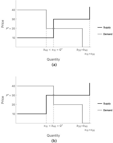
In an experimental market, half (or approximately half) of students will be assigned the role of buyer and the other half the role of seller. Buyers are assigned either a value of 40 or 20 for the good. Sellers are assigned either a value of 30 or 10. Let b₄₀ and b₂₀ denote the number of buyers assigned the values of 40 and 20, respectively. Similarly, let s₃₀ and s₁₀ denote the number of sellers assigned the values of 30 and 10, respectively. In figure 1, we depict the resulting supply and demand in the market for the two main cases of interest. In figure 1(a), we depict the case where the number of buyers with a value of 40, b₄₀, is less than the number of sellers with a value of 10, s₁₀. In this case, the equilibrium price is 20, and the equilibrium quantity is s₁₀. For instance, figure 1(a) could capture an experiment with 19 students where there are 4 buyers with a value of 40, 5 buyers with a value of 20, 5 sellers with a value of 10, and 5 sellers with a value of 30. In figure 1(b), we depict the case where the number of buyers with a value of 40, b₄₀, is more than the number of sellers with a value of 10, s₁₀. In this case, the equilibrium price is 30, and the equilibrium quantity is b₄₀.² For instance, figure 1(b) could capture an experiment with the same 19 students where there are 5 buyers with a value of 40, 4 buyers with a value of 20, 4 sellers with a value of 10, and 6 sellers with a value of 30.

Figure 1. Depiction of supply and demand for the two main cases of interest.

We will discuss the interpretation of the market in more detail shortly. Beforehand, we outline the basic protocol for running the experiment in a class:

• Based on the number of students in the room, the session leader determines the supply and demand in the market, i.e., the number of buyers and sellers with each value. (The appendix provides some advice on how to do this.)

• The correct number of cards/slips of paper stating the role, buyer or seller, and value are put in a box. Students randomly (without replacement) each pick up a card/slip of paper and keep it for the market duration.

• Once all cards are distributed, the market is opened. Students mingle around the room and try to make a deal by agreeing on a price. A seller can sell at most one good, and a buyer can buy at most one good.

• If a trade is made, the traded price, the value of the buyer, and the value of the seller are fed back to the session leader to record.

• Trading continues until either trading has ceased or a pre-determined cutoff time is reached.

• The session leader sets out the prices traded on the whiteboard or similar posting and gives relevant feedback.

• Repeat markets are conducted. We suggest running a second market with the same supply and demand and then a third market with a different supply and demand. In all markets, roles are randomly allocated afresh.

The experiment is simple to run. It should be possible to run three markets or rounds together with class feedback in 30 to 40 minutes. The experiment is also set up so that the equilibrium price and quantity are easy to determine. As illustrated in figure 1, the equilibrium price and quantity are determined by the relative number of buyers, with a value of 40, and sellers, with a value of 10. If the number of buyers with a value of 40 is less than the number of sellers with a value of 10, then the equilibrium price is 20 [figure 1(a)]. If the number of buyers with a value of 40 is greater than the number of sellers with a value of 10, then the equilibrium price is 30 [figure 1(b)]. This makes it relatively easy to determine an appropriate supply and demand at the start of the class. In particular, the number of buyers with a value of 40 and sellers with a value of 10 can be determined beforehand, and any adjustment for “late students” can be handled by sequentially adding buyers with a value of 20 and sellers with a value of 30 (without influencing the equilibrium).

The main purpose of the experiment is to illustrate supply and demand. Once all markets have been run and the prices recorded, students can be told how many buyers and sellers of each type existed in the market. Supply and demand curves can then be derived and plotted in the class to calculate the equilibrium price and quantity, as illustrated in figure 1 (Bergstrom and Miller 1999; Bergstrom and Kwok 2005). Let P_r* and Q_r* denote the equilibrium price and quantity in the market or round r. From this, one can derive predictions of what should happen:

1. There will be Q_r* trades in round r,

2. Each trade will be at price P_r* in round r,

3. All buyers with a value of 40 and all sellers with a value of 10 should trade in every round,

4. If P_r* = 20 in round r, then no seller with a value of 30 should trade, while if P_r* = 30 in round r, then no buyer with a value of 20 should trade,

5. The average trade price will be P_r* in round r,

6. If P_r* > P_r* in rounds r and r′, then the average traded price is higher in round r than r′.

Note that (a) and (b) are relatively strong predictions while (c) and (d) and then (e) and (f) are progressively weaker. (Put another way, if (a) and (b) hold, then (c) and (d) hold. Similarly, if (b) holds, then (e) and (f) must hold, and if (e) holds, then (f) holds.) The predictions (c) and (d) make clear that market equilibrium is not just about price and quantity but also about who will trade. This, as we will discuss in the social welfare section, has social welfare implications.

In the results section, we will pick out specific issues that arise in evaluating predictions (a–f). At this point, we highlight a general need, when discussing the experiment with students, to be careful in the language used around market equilibrium. The equilibrium is the “theoretical equilibrium” obtained from an assumption of market clearing around supply equals demand. Based on the theory, we can predict that the traded prices in the market will be close to equilibrium. A comparison of traded prices with equilibrium opens up the possibility of discussion on the relationships among assumptions, theory, and prediction. Specifically, if the traded prices are a long way from equilibrium, students tend to claim the “theory does not work,” “the theory is wrong,” the theory is useless,” etc. More precisely, the predictions derived from the theory have proved to be poor predictors of outcomes. One can then explore with students why that was, with reference to the assumptions of the theory and how they relate to a classroom experiment. Our experience is that students enjoy the experiment a lot because of its simplicity, combined with the class interaction and bargaining that comes from trying to buy or sell. This interaction and class engagement can then provoke an interesting discussion.

Results

We analyzed data from 85 experimental sessions collected through the use of the experiment over many years. As table 1 summarizes, there were 46 experimental sessions where the equilibrium price was 30 in rounds 1 and 2 and then 20 in round 3, i.e., a market consistent with figure 1(b) in rounds 1 and 2 and figure 1(a) in round 3. We refer to these as HHL (high, high, low equilibrium price) sessions. In such sessions, the equilibrium quantity was weakly decreasing over the three rounds. There were 27 sessions where the equilibrium price was 20 in rounds 1 and 2 and then 30 in round 3, i.e., a market consistent with figure 1(a) in rounds 1 and 2 and figure 1(b) in round 3. We refer to these as LLH sessions. In such sessions, the equilibrium quantity was weakly increasing over the three rounds. There were two sessions with no change of equilibrium, five sessions that lasted only two rounds, and five sessions with at least one market with no clear equilibrium price. These 12 sessions did not “go to plan” but still contain valid data. Overall, we have data from 114 markets with an equilibrium price of 20 and 129 markets with an equilibrium price of 30.

Table 1. Summary of equilibrium price over the three rounds in each session, together with the number of sessions.

Name	Round 1	Round 2	Round 3	Number
HHL session	30	30	20	46
LLH session	20	20	30	27
Miscellaneous sessions	30	30	30	1
	20	20	20	1
	30	30	No market	1
	30	20	No market	3
	20	20	No market	1
	30	30	Indeterminate	1
	20	20	Indeterminate	2
	Indeterminate	20	Indeterminate	1
	Indeterminate	Indeterminate	20	1

In both the HHL and LLH sessions, the market was identical in rounds 1 and 2, and then either demand, supply, or both were shifted in round 3.³ Students were aware that the market was the same in rounds 1 and 2 and shifted in round 3 (although, in all cases, they knew only their own buyer or seller value). Our data can be compared with those of Bergstrom and Kwok (2005). They provide data for 31 sessions in which there were four rounds: rounds 1 and 2 with an equilibrium price of 20 and rounds 3 and 4 with an equilibrium price of 30. These sessions are thus directly comparable to our LLH sessions. Similarities and differences in our approach are discussed more fully in the experimental design considerations section.

Trading prices

We start the analysis by evaluating prediction (f). In figure 2, we plot the average trading price over the three rounds for the HHL and LLH sessions. One can see that the average trading price increases or decreases in round 3 as predicted. While it is reassuring to see this tendency at the aggregate level, the more important question for a lecturer is what typically happens at the session level. One key measure is whether we observe the predicted change in market price between rounds 2 and 3. In 41 of the 46 HHL sessions, the average price in round 3 was, as predicted, lower than the average price in round 2. Similarly, in 24 of the 27 LLH sessions, the average price in round 3 was higher than the average price in round 2. This means that in 90 percent of the sessions, the comparative static prediction of changes between rounds 2 and 3 proved accurate. The lecturer can, therefore, be relatively confident in observing the comparative static prediction (f).

Figure 2. Average trading price in HHL and LLH sessions.

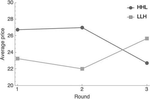
Another interesting measure to analyze is whether the equilibrium price in round 2 was closer to the market equilibrium than in round 1. This might be expected if the market converges toward equilibrium. If we look at average prices (see figure 2), there is evidence of convergence. For instance, in the LLH sessions, the average price dropped from 23.3 in round 1 to 22.0 in round 2 and therefore is getting closer to the market equilibrium price of 20. At a session level, however, the evidence for convergence is less compelling. We find that prices converge in only 26 HHL sessions and 14 LLH sessions. Hence, in only 55 percent of the sessions, we observe convergence toward equilibrium. This finding is broadly consistent with that of Bergstrom and Kwok, who report average prices of 21.2 in both rounds 1 and 2 of their experiments.

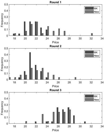
While we do not find compelling evidence of convergence to market equilibrium, there is evidence of convergence to a price above market equilibrium. To illustrate this, in figure 3, we plot the distribution of average trading prices in our LLH sessions (labeled New) and those of Bergstrom and Kwok (labeled BK). Comparing rounds 1 and 2, one can see that Bergstrom and Kwok find a tendency toward an average price of 21. While the effect is less pronounced in our data, there is still a discernible clustering of average prices in round 2, around 21 to 23. We thus seemingly observe a dynamic learning effect, but not one that is guaranteed to result in convergence to market equilibrium. Instead, it seems that prices remain slightly above equilibrium. Vernon Smith (1962) found that prices remained consistently above equilibrium with a perfectly elastic supply (see his Chart 4). The discrete nature of the market, with only two types of buyers and two types of sellers, may, therefore, be a reason for prices not readily converging fully to equilibrium.

Figure 3. Distribution of average trading price in Bergstrom and Kwok (2005) (BK) and our LLH sessions (new).

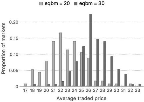
We next look at the average price in the 243 markets for which there is a unique market equilibrium (combining data from rounds 1 through 3). In figure 4, we plot the distribution of average traded prices in the market. It can be seen that if the equilibrium price is 20, then the average price is primarily in the range of 21 to 25 (68% of markets). If the equilibrium price is 30, then the average price is primarily in the range 25 to 29 (72% of markets). It is rare (about 5% of markets) that the average price is equal to market equilibrium, so prediction (e) finds little support. This can be a way to open debate about economic prediction and how we judge economic predictions (Bergstrom and Kwok 2005). On the other hand, the traded price rarely equals the market equilibrium. But, it is typically “close” to market equilibrium, and the comparative static prediction between rounds 2 and 3 is likely to hold.

Figure 4. Average traded price in the market.

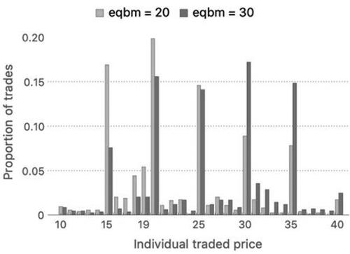
Figure 5 plots the distribution of individual trades for the 243 markets with a unique market equilibrium. There are 1588 trades in total.⁴ It can be seen that there is a pronounced pattern of trading at multiples of 5. This is consistent with a behavioral bias for round numbers. Only 15 to 20 percent of trades happen at the equilibrium price, giving little support for prediction (b). We see a strong rejection of the law of one price with a wide distribution of trading prices (Pratt, Wise, and Zeckhauser 1979; Lamont and Thaler 2003). It is possible to engage students in a discussion as to why the law does not hold. The most plausible economic answers are (i) search costs and (ii) fairness. To illustrate, consider two students, one a buyer with a value of 40 and another a seller with a value of 30, who meet in one corner of the room and start haggling. They agree to trade at 35, even though deals are being done elsewhere in the room at a price of 20. Here, we observe search costs because it is easier to do the deal than to search for a better one. Chamberlin (1948) refers to these as submarkets. We also observe “fairness” in the sense that a buyer and a seller split the surplus. In this case, the buyer with a value of 40 is not exercising her market power to drive down the price.

Figure 5. Individual trading prices in markets.

Bergstrom and Kwok (2005) explore the notion of a profit-splitting theory as an alternative to the competitive equilibrium theory. Informally, the profit-splitting theory assumes that students meet at random and trade, if possible, at a price that splits the profit between them. For instance, if a buyer with a value of 40 meets a seller with a value of 10, they trade at a price of 25. If a buyer and seller cannot trade at a profit, then they randomly seek another seller or buyer. In tables 2 and 3, respectively, we detail LLH and HHL session data on the average price for each type of buyer-seller interaction and the proportion of trades consistent with market equilibrium and profit-splitting. For example, in round 1 of the LLH sessions, there were 64 trades between a buyer of value 20 and a seller with value 10; the average price of these trades was 17.36, 16 percent of the trades were at the equilibrium price of 20, and 41 percent at the profit-splitting price of 15. The results in tables 2 and 3 show evidence of profit-splitting. In particular, around 30 percent of the trades are as predicted with profit splitting compared to only around 17 percent consistent with market equilibrium. Clearly, however, not all trades were profit-splitting. These findings are consistent with those of Bergstrom and Kwok. The lecturer may, therefore, want to compare and contrast the profit-splitting theory and competitive equilibrium theory as an illustration of evaluating competing theoretical models of behavior, with neither working “perfectly.”

Table 2. Number of trades in LLH sessions by type, average price, proportion consistent with market equilibrium, and proportion consistent with profit splitting.

		20 & 10	20 & 30	40 & 10	40 & 30	Overall
Round 1	Count	64	7	81	26	178
	Average	17.36	24.29	24.07	35.52	23.34
	Equilibrium	0.16	0.14	0.21	0.00	0.16
	Profit split	0.41	0.43	0.17	0.50	0.31
Round 2	Count	51	2	93	14	160
	Average	17.32	27.00	23.02	31.14	21.96
	Equilibrium	0.16	0.00	0.27	0.14	0.22
	Profit split	0.35	0.00	0.28	0.50	0.32
Round 3	Count	17	6	83	42	148
	Average	17.74	24.83	24.31	30.71	25.40
	Equilibrium	0.06	0.00	0.13	0.31	0.17
	Profit split	0.35	0.00	0.28	0.19	0.25

Table 3. Number of trades in HHL sessions by type, average price, proportion consistent with market equilibrium, and proportion consistent with profit splitting.

		20 & 10	20 & 30	40 & 10	40 & 30	Overall
Round 1	Count	44	11	147	101	303
	Average	17.35	27.18	24.92	33.42	26.74
	Equilibrium	0.00	0.09	0.22	0.18	0.17
	Profit split	0.41	0.09	0.17	0.37	0.27
Round 2	Count	32	14	144	113	303
	Average	18.69	28.64	25.94	31.91	27.53
	Equilibrium	0.03	0.00	0.24	0.16	0.18
	Profit split	0.22	0.36	0.30	0.41	0.33
Round 3	Count	100	16	126	61	303
	Average	17.73	21.88	24.16	32.21	23.54
	Equilibrium	0.22	0.19	0.23	0.06	0.19
	Profit split	0.37	0.13	0.26	0.48	0.34

Quantity traded

In figure 6, we plot the deviation of observed quantity traded relative to market equilibrium for the 243 markets with a unique market equilibrium. The main thing we highlight is a tendency to have a larger number of trades than at market equilibrium. This happens in around two-thirds of the markets. One can see that there is no discernible difference between markets with an equilibrium of 20 or 30. Excess trading was observed by Chamberlin (1948) and Bergstrom and Kwok (2005) and is consistent with profit-splitting theory (Bergstrom 2004). A related explanation for why we observe more trades than in equilibrium is that students want to participate in the experiment, creating a bias toward trade (and profit-splitting). We told students that they need not trade, and some students showed a reticence toward trade. That we observe more trades than at equilibrium is, therefore, a positive signal that students are willing to engage in the experiment. Note that, on average, 70 percent of students would have traded according to market equilibrium, and 80 percent of students actually traded in the market. Over the course of three rounds, the vast majority of students, therefore, trade at least once.

Figure 6. Deviation of quantity from equilibrium.

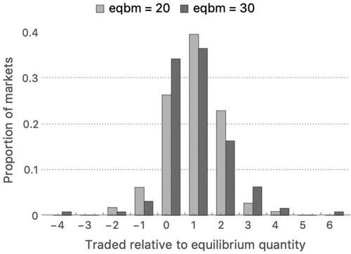
Recall that supply and demand analysis makes clear predictions on who should trade in equilibrium, prediction (c), and who should not trade, prediction (d). Reflecting these predictions, we refer to “unanticipated abstinence” if a buyer with a value of 40 or a seller with a value of 10 does not trade. Similarly, we refer to “unanticipated trading” if a seller will value 30 trades when the equilibrium price is 20 and a buyer will value 20 trades when the equilibrium price is 30. In table 4, we detail the size of unanticipated abstinence and unanticipated trading in our experimental markets. In 69.3 percent of markets, we do not observe any unanticipated abstinence, and in 27.1 percent of the markets, there is only one unanticipated abstinence. The lecturer can, therefore, expect to find strong support for prediction (c). By contrast, we observe no unanticipated trades in only 30.1 percent of the markets. In most markets, therefore, we observe at least one unanticipated trade, suggesting little support for prediction (d). This combination of trading by those predicted to trade and some trading by those predicted not to trade explains the excess trading observed in figure 6. It is also consistent with the profit-splitting theory and the desire of students to trade and participate in the experiment.

Table 4. Proportion of markets (%) in which the given number of students with values 40 and 20 do not trade (unanticipated abstinence) and in which the given number of students with values 20 or 30 trade when not predicted (unanticipated trading).

	Unanticipated abstinence			Unanticipated trading
Number	P* = 20	P* = 30	Overall	P* = 20	P* = 30	Overall
0	74.0	65.3	69.3	33.0	27.7	30.1
1	24.0	29.7	27.1	38.0	38.7	38.4
2	1.0	1.7	1.4	25.0	23.5	24.2
3	1.0	3.4	2.3	3.0	7.6	5.5
4	0.0	0.0	0.0	1.0	2.5	1.8
5	0.0	0.0	0.0	0.0	0.0	0.0

Social welfare

We believe that the natural inclination of most students is to think that more trades than equilibrium is welfare improving. The experiment provides, therefore, an excellent starting point for a discussion on the First Theorem of Welfare Economics, namely that market equilibrium yields Pareto efficiency and shows that market equilibrium maximizes social welfare. We use the standard definition of social welfare as the total surplus in the market (i.e., consumer surplus plus producer surplus). In our experiments, the average surplus as a proportion of the equilibrium surplus was around 90 percent (92% with an equilibrium price of 20 and 90% with an equilibrium price of 30). Thus, 10 percent of the surplus was lost due to excess trades.

To give an example that can be used during the discussion: Suppose there are five sellers with a value of 10, five with a value of 30, and five buyers with a value of 20, and four with a value of 40. In equilibrium, there should be five trades at price 20 consisting of the four buyers with a value of 40 and one buyer with a value of 20 trading with sellers with a value of 10. That gives a total surplus of 4 × 30 + 1 × 10 = 130. In figure 7, this is the area between the supply and demand curve left of the market equilibrium. Now, suppose that we have six trades consisting of three buyers with a value of 40 and two with a value of 20 trading with sellers with a value of 10, and one buyer with a value of 40 trading with a seller with a value of 30. The total surplus drops to 3 × 30 + 3 × 10 = 120. On the diagram, we can represent this by artificially moving one of the buyers with a value of 40 to the right of the equilibrium. In this case, we obtain two trades that are not consistent with market equilibrium. These trades are profitable for both the buyers and sellers involved but ultimately lower total surplus compared to market equilibrium.

Figure 7. A diagram that illustrates the loss of surplus if there are two trades not predicted by market equilibrium: a buyer with a value of 40 trades with a seller with a value of 30, and there is an extra trade between a buyer with a value of 40 and seller with a value of 10.

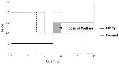
This example may seem counterintuitive, so it is worth providing time to go through the example slowly, allowing students to “discover for themselves” why there is a loss of surplus. The discussion could then turn to issues of fairness and potentially the Second Theorem of Welfare Economics. In the example, the “extra” seller with a value of 30 gains from being able to trade with a buyer that has a value of 40. For instance, suppose she sells at a price of 35. She then has gained 5 relative to the market equilibrium (where she does not trade). The tradeoff is that the buyer sees his surplus drop 15, from 20 at market equilibrium to 5 with this trade. Some might argue this outcome is “fairer” because one more person gains by being able to trade. That depends on the definition of fairness used (e.g., Rawlsian versus utilitarian). In terms of the Second Theorem of Welfare Economics, a “better solution” would be for the buyer with a value of 40 to obtain a surplus of 20 (as in market equilibrium) and then “donate” 10 to the seller with a value of 30. This maximizes and redistributes surplus.

Experimental design considerations

As already mentioned, the experiment we are discussing in this article is a minor variant of that set out by Bergstrom and Miller (1999) and discussed by Bergstrom and Kwok (2005). Within the basic framework of the experiment, there are a number of design elements that can potentially influence outcomes, which the lecturer may want to consider. In this section, we explore some of those elements and, in doing so, further compare our results with those of Bergstrom and Kwok.

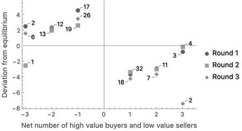
One crucial issue to consider is the balance of the market between high- and low-valuation buyers and sellers. Recall (see figure 1) that the equilibrium price depends on whether the number of buyers with a value of 40 is greater than the number of sellers with a value of 10. Define NH as the number of buyers with a value of 40 minus the number of sellers with a value of 10. That is, NH = b₄₀ – s₁₀. The absolute value of NH could be seen as a measure of the “balance of power” between buyers and sellers. In our markets, we typically set up the market so that NH = 1 or −1, meaning that the balance of power favored only buyers or sellers, respectively. This was done to provide a transparently “tough test” of competitive equilibrium predictions (a–f). The lecturer may, though, want to “play safe” and have a larger NH. Indeed, Bergstrom and Kwok advocate a larger NH of absolute size over 5. In figure 8, we plot the relationship between NH and the deviation of the average traded price from the equilibrium price in our data. The upper trend suggests that a larger absolute value of NH does appear to result in a smaller deviation from equilibrium. This effect is highly statistically significant when the equilibrium price is 20 (p = 0.002 Mann Whitney test of NH = −1 versus NH < −1), but not when the equilibrium price is 30 (p = 0.12 Mann Whitney test of NH = 1 versus NH > 1).

Figure 8. Deviation of average traded price from equilibrium as a function of the number of high-value buyers minus low-value sellers for each round of the experiment. The number of observations is provided for each data point.

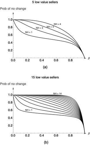
To explore this issue further, we considered the sensitivity of equilibrium to student engagement in the class. Specifically, suppose that independently, with probability p, each student disengages from the experiment and makes no effort to trade (either because they are distracted, confused, or unwilling, etc.). This disengagement can shift the “effective” supply and/or demand curve (relative to the assumed experiment supply and demand curve) and, thereby, potentially change the effective equilibrium price. For instance, suppose NH = 1, meaning the assumed equilibrium price is 30, but two buyers of a value of 40 disengage from the experiment. This shifts the effective demand curve to the left and results in an effective equilibrium price of 20. The probability of the effective equilibrium price being the same as the assumed market price can be calculated as a function of p and NH.⁵

In figure 9, we plot the probability of no change in equilibrium when there are, respectively, 5 and 15 sellers with a value of 10. One can see that if |NH| = 1, a small amount of disengagement can shift the effective equilibrium, while for larger |NH|, the effective equilibrium is unlikely to change. To provide an estimate of p for our data, we note that 4.1 percent of students with values of 40 and 10 do not trade (unanticipated abstinence). Given that such students should be able to trade, we suggest that this can be used as a measure of disengagement, giving p = 0.41. The lecturer concerned about trading price being too far away from market equilibrium may, therefore, prefer to set NH greater than 1 or 2 in absolute value. We suggest (see the online appendix) setting NH between 2 and 5, depending on class size.

Figure 9. Probability of effective market equilibrium not changing if students disengage from the experiment with probability p, comparing a setting with 5 and 15 sellers of a value of 10.

Overall, we discern four potentially important differences between the design of our experiment and those reported in Bergstrom and Kwok (2005):

1. Our experiments used a marginal balance of power with NH close to 1 in absolute value, while Bergstrom and Kwok consider a larger value of NH.

2. Our experiments have a smaller number of students (typically 15 to 25) compared to Bergstrom and Kwok.

3. In the transition from round 2 to round 3, we consider a relatively small change in either the demand or supply curve (keeping NH close to 1 in absolute value), while Bergstrom and Kwok consider a larger shift in both demand and supply curves.

4. In our experiment, prices were reported only once the market had closed, while in Bergstrom and Kwok, they were reported live as they happened.

Apriori, one would expect all four of the differences described above to result in more divergence from competitive equilibrium in our experiments. For instance, we have already discussed how a smaller NH increases deviation from equilibrium. Crucially, despite these differences, the results we obtain in our experiments are very similar to those of Bergstrom and Kwok. Figure 3 shows that the prices we observe, while slightly more dispersed than Bergstrom and Kwok’s, are similar. The corresponding data for deviation of quantity from market equilibrium are also strikingly similar across our experiments and that of Bergstrom and Kwok (data available on request). We suggest, therefore, that the outcomes of the classroom experiment are not overly sensitive to the specifics of the design. This is reassuring and speaks to the merit of the experiment.

We finish the analysis with consideration of the number of students in the class. If, as the profit-splitting theory suggests, trades happen as individuals randomly interact, the distribution of individual trades should be the same for different market sizes. This means, however, applying the law of large numbers argument that the average traded price would be less dispersed in larger classes. To illustrate, in figure 10, we plot the predicted average traded price for a market size of 10 compared to a market size of 30 when the equilibrium price is 20. This prediction is based on a random sampling of the observed prices in our experiments. It can be seen that a larger class size results in a narrowing of the distribution, consistent with that seen in figure 3 when comparing our results with Bergstrom and Kwok.

Figure 10. Predicted average traded price when market equilibrium is 20 comparing a market size of 10 with a market size of 30.

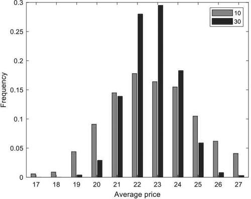
Putting these findings together, we suggest that the observed differences between our distribution of average prices and that of Bergstrom and Kwok can be explained by (i) our use of a smaller absolute value of NH, which led to prices being slightly further from market equilibrium, and (ii) smaller class sizes, which led to the distribution being slightly more dispersed. These are effects the lecturer can take into account when deciding on the design they want to adopt for their experiments.

Conclusion

In this article, we have analyzed data accumulated over many years from teaching a market interaction classroom experiment to first-year undergraduate students. We believe that more feedback and data on completed experiments may encourage a wider set of faculty to take up the use of classroom experiments. In particular, it means we can provide a “full package” of details, from how to run the experiment to comprehensive insight into what is likely to happen during an experiment. We have seen that some predictions derived from market equilibrium are likely to work well, e.g., comparative static predictions on changes in price, and some that will not, e.g., the law of one price. We have also shown that deviations of observed outcomes from equilibrium outcomes can be a useful way to provoke discussion around issues such as the fairness of markets.

The fact that we observe significant deviations from market equilibrium is consistent with our experimental design deviating from the double-auction benchmark. Specifically, abundant evidence suggests that double auctions are efficient, with traded prices and quantity very close to market equilibrium, while deviations from double auctions lead to market inefficiency (e.g., Smith et al. 1982; Ketcham, Smith, and Williams 1984). Classroom experiments using double auctions are likely to lead to more “straightforward” results (Lin et al. 2020). As discussed by Holt (1996), there is, therefore, something of a tension between the “Chamberlin (1948) approach” that we have followed, where deviations from equilibrium are expected, versus settings with more transparent information where trading is more likely to converge to equilibrium.

One thing to remark about this tension is that the instructor has an array of design factors that can be varied to move from one extreme to the other. We would highlight that the findings in our experiments are very consistent with those of Bergstrom and Kwok (2005), even though our experiments provide a “tougher” environment for market equilibrium convergence. The lecturer can, therefore, be reassured that the success of the experiment is not overly dependent on the choice of design. That said, there are tradeoffs the lecturer can consider. In the experimental design considerations section, we considered class size and the balance of power between buyers and sellers. Also, in our experiment, trades take place all over the room, and prices are revealed only once all trades in that market are done. In Holt’s (1996) and Bergstrom and Kwok’s (2005) designs, trades take place in a specific area of the room, and prices are revealed as they are done. The instructor that would like a closer fit with market equilibrium therefore has tools to help bring that about.

We finish by noting that a further fundamental aspect of experiment design to consider is whether to use a pen-and-paper experiment or a computer-aided experiment. Giamattei and Llavador (2017) show how market experiments like those used in Bergstrom and Miller (1999) can be facilitated by digital technology. Their approach still entails face-to-face physical interaction with results inputted onto the mobile device. This can facilitate the running of the experiment at larger scales and make the lecturer’s task easier. More generally, platforms like o-Tree provide an accessible medium for lecturers to design and run online market-based experiments with remote interaction. It is an open question whether results are similar online or using pen and paper (e.g., Carter and Emerson 2012).

Appendix availability

The online appendix is available at https://figshare.com/articles/online_resource/‌Online_Appendix_for_A_Classroom_Market_Experiment_Data_and_Reflections_/22100369

Acknowledgments

Both authors contributed equally to this work. They thank an anonymous referee and the journal’s associate editor for their contributions to improving the article.

Disclosure statement

No potential conflict of interest was reported by the author(s).

Data availability statement

The data analyzed in this article are available at https://figshare.com/articles/‌dataset/Data_file_for_paper_A_Classroom_Market_Experiment_Data_and_Reflections_/22104740

Notes

1 https://figshare.com/articles/online_resource/Online_Appendix_for_A_Classroom_Market_‌Experiment_Data_and_Reflections_/22100369.

2 If b₄₀ = s_10, then the equilibrium price is undetermined. Hence, this outcome is best avoided in the experiment.

3 The only exception was that if students arrived after round 1 had started, and were thus added to round 2. This was done in a way that did not influence the market equilibrium price and quantity.

4 Not plotted on this figure are one trade at price 1, one trade at price 41, two trades at price 45, and three trades at price 50.

5 If there are s₁₀ sellers with a value of 10 and b₄₀ buyers with a value of 40, and s₁₀ > b_40, then the probability that the market equilibrium is 20 is given by ${\sum }_{x=1}^{{\mathrm{s}}_{10}}{\sum }_{y=0}^{\mathrm{\text{min}}(x-1,{\mathrm{b}}_{40})}\left(\begin{array}{c}{\mathrm{s}}_{10}\\ x\end{array}\right)\left(\begin{array}{c}{\mathrm{b}}_{40}\\ y\end{array}\right){(1-p)}^{x+y}{p}^{{\mathrm{s}}_{10}+{\mathrm{b}}_{40}-x-y}$.

References

- Allgood, S., W. B. Walstad, and J. J. Siegfried. 2015. Research on teaching economics to undergraduates. Journal of Economic Literature 53 (2): 285–325. doi: 10.1257/jel.53.2.285.
- Bergstrom, T. C. 2004. Experimental markets and Chamberlin’s excess trading conjecture. Ted Bergstrom Papers. Santa Barbara, CA: University of California, Santa Barbara.
- Bergstrom, T. C., and E. Kwok. 2005. Extracting valuable data from classroom trading pits. Journal of Economic Education 36 (3): 220–35.
- Bergstrom, T. C., and J. Miller. 1999. Experiments with economic principles: Microeconomics. New York: McGraw-Hill/Irwin.
- Carter, L. K., and T. L. Emerson. 2012. In-class vs. online experiments: Is there a difference? Journal of Economic Education 43 (1): 4–18.
- Chamberlin, E. H. 1948. An experimental imperfect market. Journal of Political Economy 56 (2): 95–108. doi: 10.1086/256654.
- DeYoung, R. 1993. Market experiments: The laboratory versus the classroom. Journal of Economic Education 24 (4): 335–51.
- Durham, Y., T. McKinnon, and C. Schulman. 2007. Classroom experiments: Not just fun and games. Economic Inquiry 45 (1): 162–78. doi: 10.1111/j.1465-7295.2006.00003.x.
- Emerson, T. L., and L. K. English. 2016a. Classroom experiments: Is more more? American Economic Review 106 (5): 363–67. doi: 10.1257/aer.p20161054.
- ———. 2016b. Classroom experiments: Teaching specific topics or promoting the economic way of thinking? Journal of Economic Education 47 (4): 288–99.
- Giamattei, M., and H. Llavador. 2017. Teaching microeconomic principles with smartphones—Lessons from classroom experiments with classEx. Working paper. Rochester, NY: SSRN-Elsevier. https://papers.ssrn.com/sol3/papers.cfm?abstract_id=3157026.
- Grol, R., E. M. Sent, and B. de Vries. 2017. Participate or observe? Effects of economic classroom experiments on students’ economic literacy. European Journal of Psychology of Education 32 (2): 289–310. doi: 10.1007/s10212-016-0287-8.
- Holt, C. A. 1996. Classroom games: Trading in a pit market. Journal of Economic Perspectives 10 (1): 193–203. doi: 10.1257/jep.10.1.193.
- Holt, C. A. 1999. Teaching economics with classroom experiments: A symposium. Southern Economic Journal 65 (3): 603–10.
- Kaplan, T. R., and D. Balkenborg. 2010. Using economic classroom experiments. International Review of Economics Education 9 (2): 99–106. doi: 10.1016/S1477-3880(15)30047-5.
- Ketcham, J., V. L. Smith, and A. W. Williams. 1984. A comparison of posted-offer and double-auction pricing institutions. The Review of Economic Studies 51 (4): 595–614. doi: 10.2307/2297781.
- Lamont, O. A., and R. H. Thaler. 2003. Anomalies: The law of one price in financial markets. Journal of Economic Perspectives 17 (4): 191–202. doi: 10.1257/089533003772034952.
- Laury, S. K., and C. A. Holt. 1999. Multimarket equilibrium, trade, and the law of one price. Southern Economic Journal 65 (3): 611–21.
- Lin, P. H., A. L. Brown, T. Imai, J. T. Y. Wang, S. W. Wang, and C. F. Camerer. 2020. Evidence of general economic principles of bargaining and trade from 2,000 classroom experiments. Nature Human Behaviour 4 (9): 917–27. doi: 10.1038/s41562-020-0916-8.
- Lin, T. C. 2018. Using classroom game play in introductory microeconomics to enhance business student learning and lecture attendance. Journal of Education for Business 93 (7): 295–303. doi: 10.1080/08832323.2018.1493423.
- Lin, T. C. 2020. Effects of classroom experiments on student learning outcomes and attendance. International Journal of Education Economics and Development 11 (1): 76–93. doi: 10.1504/IJEED.2020.104295.
- Pratt, J. W., D. A. Wise, and R. Zeckhauser. 1979. Price differences in almost competitive markets. The Quarterly Journal of Economics 93 (2): 189–211. doi: 10.2307/1883191.
- Smith, V. L. 1962. An experimental study of competitive market behavior. Journal of Political Economy 70 (2): 111–37. doi: 10.1086/258609.
- Smith, V. L., A. W. Williams, W. K. Bratton, and M. G. Vannoni. 1982. Competitive market institutions: Double auctions vs. sealed bid-offer auctions. The American Economic Review 72 (1): 58–77.