Mixing coefficients for longitudinal and vertical mixing in the near field of a surface pollutant discharge

Abstract

Laboratory experiments conducted in a rectangular open channel on passive mixing of pollutants in longitudinal and vertical directions due to a transverse line source on the flow surface are reported. A finite numerical difference scheme developed by the authors was extended to determine optimum values of longitudinal and vertical mixing coefficients from the observed concentration versus time curves. The vertical mixing coefficient was also computed from the measured velocity distribution and compared with the derived optimum. The velocity distribution-based values of vertical mixing coefficient corresponds well with the optimum derived using the numerical scheme. Through a sensitivity analysis, the errors in the predicted concentration versus time curves are quantified by using the numerical scheme proposed by the authors for two-dimensional dispersion in streams. The sensitivity analysis indicated that predictions of concentration versus time curves can be made with a maximum error of about ±30% if a ±100% error is contained in the values of longitudinal and vertical mixing coefficients.

Keywords:

• Mixing coefficient
• open channel flow
• passive mixing
• slug source
• transverse mixing

1 Introduction

Prediction of pollutant concentration downstream of the injection point is required for assessing the impact of industrial and municipal waste disposal schemes into a stream system. For a transverse line pollutant source, the mixing is in the near-field mainly in the vertical and longitudinal directions, whereas only longitudinal mixing occurs in the far-field region. However, even for a transverse line source, a tracer gets distorted in the initial phase due to transverse velocity as a result of the transverse mixing. Even though the vertical mixing occurs only near the source, the understanding of vertical mixing is essential to determine the pollutant concentration in the far-field region. Compared with transverse and longitudinal mixing, the vertical mixing was not studied extensively (Schiller and Sayre 1975, French 1979, McNulty and Wood 1984, Nokes and Wood 1988). Dumping of the pollutants across streams from a bridge, the disposal of hot water from thermal power plants into a stream, and the bursting of a pipe carrying pollutants across a water body are examples which resemble the process of transverse line slug mixing in streams (Kim and Seo 2000, Khan et al. 2007).

The equation governing the mixing of conservative pollutants in the longitudinal and vertical directions from a transverse line slug source in open channels is (Nokes et al. 1984)

where x and y are the longitudinal and vertical distances, respectively, C the width-averaged pollutant concentration, t the time, U the width-averaged longitudinal velocity, E _x the longitudinal mixing coefficient, and E _y the vertical mixing coefficient. The predicted concentration profiles are not sensitive to the vertical distribution of E _y and for typical practical problems, the depth-averaged value of is used (Elder 1959, Jobson and Sayre 1970a, 1970b, Seo et al. 2006). Accordingly

where d is the flow depth and U _* the shear velocity. The longitudinal dispersion coefficient relevant in one-dimensional (1D) mixing accounts for the velocity defect from the cross-sectional average velocity, while E _x accounts for the velocity defect in the lateral direction from the width-averaged velocity at a given depth. Thus, values of these coefficients are different as they result from different processes. However, there is a need to quantify the variation of E _y along the vertical direction to decide if E _x along the flow depth may also be discerned to be constant.

Numerical solutions of Eq. (1) or its simplified form for the different boundary conditions are available in the literature, such as Nokes et al. (1984), Stefanovic and Stefan (2001), Tsai et al. (2002), Guan et al. (2002) and Seo et al. (2008). Singh et al. (2009) solved Eq. (1) using the finite difference scheme, based on the split-operator approach, for a transverse line slug source. They also validated the proposed scheme with benchmark analytical and experimental results. Shiono et al. (2003) used turbulence models to predict solute distributions in an asymmetric compound channel.

This study aims at conducting laboratory experiments on the passive mixing of pollutants in longitudinal and vertical directions due to a transverse line source in a rectangular open channel. Optimum values of these coefficients for two-dimensional (2D) mixing are thus obtained by coupling the experimental observations with the numerical model developed concurrently by Singh et al. (2009). The sensitivity of the predicted C-t curves to the possible presence of errors in E _x and E _y are also checked. Finally, recommendations are made for practice.

2 Experimental program

2.1 Test set-up

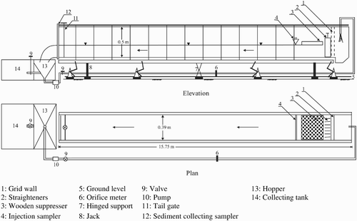
Experiments were carried out at the Hydraulics Laboratory of Indian Institute of Technology, Roorkee (India) in a recirculating tilting flume, 15.75 m long, b = 0.39 m wide and 0.50 m deep (Fig. 1). The flume was provided with transparent glass walls on both sides and cement plaster on the bottom. The side wall correction of Einstein (1942) was applied to compute the hydraulic radius R _b relative to the bottom (subscript b). Flow straighteners were provided and two mesh walls were placed upstream of the straighteners to reduce large size eddies. A perforated wooden wave suppressor was provided after the straighteners to damp surface waves.

Figure 1 Layout of experimental set-up

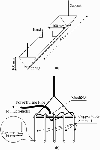
Water was supplied to the flume using a valve for regulating the discharge, and a sector orifice meter for measuring the discharge. Water samples were taken continuously from the flume and passed through a Fluorometer 10 AU-005, Turner Designs Sunnyvale^®, to measure the tracer concentration C. The C–t curves were measured at a temporal resolution of 1 s. The flow velocity across the monitoring system was kept equal to the channel flow velocity to minimize further dispersion of the dye while the flow entered into the Fluorometer. The density of the concentrated Rhodamine WT fluorescent dye, used as tracer herein, was 1190 kg/m³. This dye was highly diluted with water before its injection to obtain equal density of both liquids to minimize the buoyancy effect. The dye was injected into the flow as a slug in the form of a transverse line source on the water surface by an injection sampler (Fig. 2a). The sampler consisted of a fixed metallic open tray of triangular cross-section 350 mm long and 100 mm high. The tracer collecting sampler shown in Fig. 2(b) consisted of five copper tubes of 8 mm diameter at 90 mm centre-to-centre spacing directed against the flow direction to cause a minimum disturbance in mixing of flow and tracer. Through the tubes, the samples entered into a manifold of 50 mm diameter and 25 mm height and finally to the Fluorometer.

Figure 2 (a) Tracer injection sampler, (b) tracer collecting sampler

2.2 Test procedure

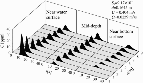
The experiments were conducted for four bottom slopes S _o and various discharges Q for each slope. For each test, a known concentration of Rhodamine WT solution was poured into the tracer injection sampler and positioned slightly above the water surface. Uniform flow was established by adjusting the tail gate rendering the water surface parallel to the channel bottom. The collecting sampler was located 1 m downstream from the injection sampler and about 5 mm above the bottom. The dye was injected instantaneously by pressing handles of the injection sampler synchronized with the data logger of the Fluorometer and data at 1 m from the injection site was recorded. Data were also collected at the mid-depth of flow and 10 mm below the water surface for equal volume of injected dye. Likewise, data were recorded in 1 m steps downstream from the injection site at identical depths. The recorded data were transferred to the computer using an Internal Data Logging software for further analysis. A typical set of the temporal variation of observed width-averaged concentration at downstream distances 1–9 m from the injection site and at three depths is shown in Fig. 3. For each run, the longitudinal velocity distribution over the depth along five verticals in the lateral direction was measured with a Prandtl–Pitot tube. The measured velocities are an important indicator of the presence of secondary currents and a lateral velocity defect. These two factors are responsible for the mixing caused by the vertical shear. The observed velocity distribution exhibits a high degree of two-dimensionality over the central region of the channel (Singh et al. 2009). A comparison of the observed distribution of vertical velocity in the middle section with the log-law indicated that the observed values were higher near the channel bottom, but smaller near the flow surface. Some tests were repeated for checking the repeatability of the observations (Singh 2005). Practically, no differences in the observed C–t curves were noticed.

Figure 3 Typical observed width-averaged tracer concentration versus time (C–t) curves

The relevant hydraulic parameters are listed in Table 1, where U ₁, U ₂ and U ₃ are the width-averaged bottom velocities, at the mid-depth and near-water surface, respectively. The average value of shear velocity was derived using S _o and R _b by estimating the sidewall corrections by Einstein's method (Garde and Ranga Raju 2006). Literature data on E _y of Jobson and Sayre (1970b), Schiller and Sayre (1973), Nokes (1986) and McNulty (1983), and the corresponding flow conditions are also listed.

Table 1 Hydraulic parameters and mixing coefficients

Sl. no.	d (m)	Q (m^3/s)	U (m/s)	R b (m)	S o	U * (m/s)	E y /dU *	E x /dU *	U 1 (m/s)	U 2 (m/s)	U 3 (m/s)
1	0.123	0.0195	0.437	0.092	9.17 × 10^−4	0.029	0.1280	54.47	0.378	0.446	0.455
2	0.155	0.0224	0.370	0.121	9.17 × 10^−4	0.033	0.1203	21.92	0.327	0.375	0.386
3	0.1785	0.0305	0.438	0.128	9.17 × 10^−4	0.034	0.9114	171.14	0.414	0.465	0.468
4	0.0895	0.0158	0.454	0.063	9.17 × 10^−4	0.024	0.1771	41.55	0.400	0.479	0.488
5	0.1645	0.0259	0.404	0.123	9.17 × 10^−4	0.033	0.0679	15.15	0.378	0.437	0.448
6	0.1005	0.0184	0.470	0.069	9.17 × 10^−4	0.025	0.0900	26.68	0.413	0.496	0.506
7	0.103	0.0198	0.492	0.068	9.17 × 10^−4	0.025	0.0617	14.20	0.364	0.420	0.428
8	0.124	0.0210	0.434	0.095	1.18 × 10^−3	0.033	0.0867	9.56	0.362	0.440	0.459
9	0.134	0.0263	0.504	0.095	1.18 × 10^−3	0.033	0.0532	7.53	0.442	0.516	0.527
10	0.145	0.0276	0.487	0.105	1.18 × 10^−3	0.034	0.0667	4.95	0.397	0.478	0.500
11	0.164	0.0318	0.498	0.117	1.18 × 10^−3	0.037	0.1364	44.72	0.405	0.486	0503
12	0.196	0.0394	0.515	0.137	1.18 × 10^−3	0.040	0.0958	16.67	0.475	0.530	0.536
13	0.15	0.0282	0.482	0.109	1.18 × 10^−3	0.035	0.1052	27.87	0.380	0.470	0.550
14	0.115	0.0263	0.587	0.087	2.00 × 10^−3	0.042	0.2490	35.20	0.495	0.590	0.602
15	0.15	0.0341	0.583	0.114	2.00 × 10^−3	0.048	0.1086	17.49	0.551	0.632	0.627
16	0.128	0.0258	0.517	0.096	1.47 × 10^−3	0.037	0.0514	4.35	0.479	0.563	0.577
17	0.147	0.0290	0.506	0.111	1.47 × 10^−3	0.040	0.0559	7.56	0.437	0.510	0.512
18	0.162	0.0318	0.503	0.123	1.47 × 10^−3	0.042	0.1280	54.47	0.461	0.522	0.526
19	0.184	0.0367	0.512	0.138	1.47 × 10^−3	0.045	0.1203	21.92	0.467	0.532	0.542
20	0.109	0.0235	0.554	0.078	1.47 × 10^−3	0.034	0.9114	171.14	0.548	0.630	0.620

3 Normalization of C–t curves

For all data sets, the recovered tracer mass at downstream stations was computed resulting in 95–99% mass recovered of the injected mass, the small difference being attributed to the experimental error. To equalize the recovered tracer mass to the injected tracer, the data at each station were normalized with respect to the average recovered mass of tracer. After deduction of the blank from the observed tracer concentration, the C–t curves were integrated. The cross-sectional area at a section was divided into three horizontal strips (sub-areas) to compute average velocity and depth. The tracer mass M recovered at a station was computed from

where N ₁ is the total number of sub-areas, ΣCΔt the integration of C–t curve, b _k and d _k the width and depth of the sub-area, respectively and U _k the width-averaged longitudinal velocity in the sub-area. The mass of the recovered tracer at the subsequent station was calculated from Eq. (3). The observed C–t curves at each station were then linearly normalized with respect to the average recovered mass of tracer.

4 Determination of mixing coefficients

The finite difference scheme developed by Singh et al. (2009) was extended to determine the values of E _x and E _y , using the observed C–t curves at y/d = 0, 0.5 and 1.0 downstream of the pollutant source. Based on the split-operator approach, Singh et al. (2009) developed a numerical scheme for the solution of the 2D mixing equation with transverse line slug source in open channel flows. A forward scheme for the temporal derivative and a backward scheme for the spatial derivative were used to solve the advection equation. The exact solution was found by adopting the Courant number equal to unity for the computational nodes on the water surface. For the other computational nodes, a cubic-spline interpolation scheme was utilized to account for the velocity defect along the vertical. Computations by the diffusion equation involved the alternate-direction implicit method, in which a forward scheme is used for the temporal derivative and either of the second-order spatial derivative was solved by using the implicit finite scheme for the given time level while the other second-order derivative was solved similarly for the next time level. To obtain a stable solution, the operational direction was reversed for the second-order derivative terms to evaluate concentration at the next time level. The scheme is mass conservative.

The results were derived based on Singh et al.'s (2009) scheme for various grid sizes noticing that the results did not vary in the range of grid sizes adopted in the study, indicating negligible numerical dispersion. The grid sizes used were of the order of Δx = 0.5 m, Δy = 0.05 m, and Δt = 1 s, and the spatial computational domain covered up to 0.196 and 40 m in vertical and longitudinal directions, respectively. Initial concentration at all grid points were taken as zero. At the upstream boundary, the observed concentration at the water surface was used and zero values of observed concentration at other nodes of the upstream boundary were used. Zero values of concentration were also taken at the downstream boundary at all elevations. A derivative boundary condition was considered both at the bottom and the water surface as no flux crosses the boundaries. The order of the longitudinal Peclet number was 175, whereas the Courant number varied from 0.7 to 1. The scheme was validated with the analytical solutions of Fischer (1968) for 1D mixing, Lipsett and Beltaos (1978) for continuous injection of pollutant as a steady transverse line source, and the laboratory data of Singh (2005) for slug injection.

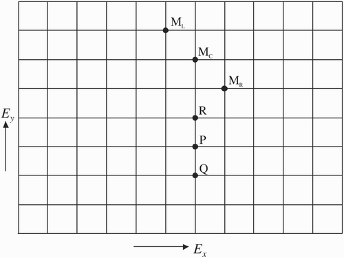
To determine the mixing coefficients, a 2D computational grid search method was employed (Fig. 4). For the grid search, an initial value of E _x was estimated using Fischer et al.'s (1979) triple integral method, while Eq. (2) was used to determine the initial value of E _y . These values were considered to be the optimum producing minimum error ERS (Ahmad and Kothyari 2001, Ahmad et al. 1999a, 1999b) defined as

For a number of C–t curves at various y-values along the vertical direction at a certain station, the weighted error was computed as

Figure 4 Computational procedure for search of optimum mixing coefficients E _x and E _y

Here A(k) is the area of observed C–t curves “k”, ERS(k) the error in C–t curves ‘k’ and N ₁ the total number of C–t curves at a station. The average error, ERR was calculated by the arithmetic mean of all weighted errors.

Within the computational domain, the search for optimum values of E _x and E _y began, say, at point P (Fig. 4) which corresponded to the initially chosen trial value of E _x and E _y and the ERR value was therefore computed first for P. The search for identifying the point corresponding to the minimum ERR was advanced in the neighbourhood of P, first along the vertical through P. Therefore incremental values equal to ±ΔE _y were added to the precedent value of E _y with ΔE _y as 1/10 of the precedent E _y value. Let the adjusted values of E _y corresponded to points Q and R, respectively (Fig. 4) and the ERR value was calculated therefore at Q and R too. If among P, Q and R, the ERR was least at P, then the computational grid was refined by taking ΔE _y (new) = ΔE _y (old)/2 and the search was repeated along the same vertical line around P until the point corresponding to the minimum ERR was identified. Instead, if ERR was lower either at R or Q, the search procedures were instead applied at thus identified position. Assuming that the search resulted in identification of the point of minimum ERR, say point M_C (Fig. 4), the value of E _x and E _y at this point would correspond to a local optimum along the computational vertical through P. For searching the global optimum values of E _x and E _y , the search was shifted alternately to both sides of M_C with a new (E _x +ΔE _x ) and next to (E _x −ΔE _x ). Repeating this search procedure, the local minima of, say, M_R and M_L (Fig. 4) were also identified. Among the three local optimum points, i.e. M_R, M_L and M_C, the one having minimum ERR was selected. If M_C corresponds to the minimum ERR, then it was considered as the global optimum value. Instead, if either M_R or M_L was associated with the lowest ERR, then the search was shifted alternatively to both sides of the point associated with the minimum ERR. Computational traversing as explained above was continued in search of the global optimum until the entire computational domain was covered. The C–t curves computed by this derived optimum value of E _x and E _y compared well with observations. Any difference between the observed and computed C–t curves that may be still residual was mainly attributed to experimental errors.

5 Verification of existing predictors for E _y

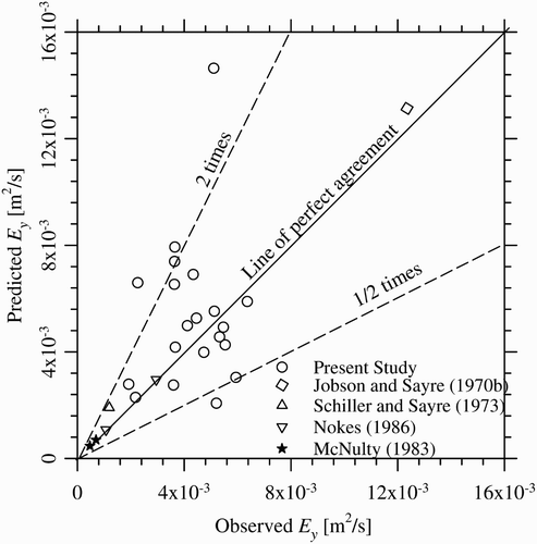
The experimental data collected in this study and the literature data were used to verify the existing predictors for E _y . These values, computed using Eq. (2) were compared with the corresponding observed (optimum) value of E _y as shown in Fig. 5. Most of the E _y values predicted by Eq. (2) lie within a range of 2–0.5 times the observed values. The values of E _y were also estimated using the measured velocity at the mid-channel width along the vertical direction (Rutherford 1994) and compared with the corresponding observed (optimum) values. The agreement between E _y computed from the vertical velocity distributions with these observed is slightly better than E _y computed using Eq. (2). Typical longitudinal velocity distributions over the flow area are given by Singh et al. (2009). Thus, the observed velocity distributions were noticed to differ slightly from the log law (Singh 2005), that was assumed in the derivation of Eq. (2). It is therefore understandable that E _y by Eq. (2) did not match very well with the observations. Therefore, E _y determined by the measured velocity distributions are used for the computations henceforth.

Figure 5 Comparison of E _y predicted by Eq. (2) with observed values

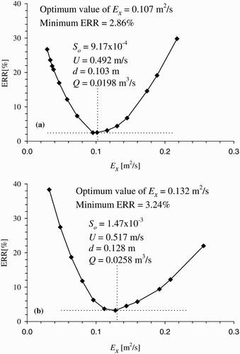
The estimated values of E _x were also re-determined by Singh et al.'s (2009) numerical scheme, using E _y obtained through the use of observed velocity distributions. Those values of E _x were considered to be the optimum corresponding to the minimum value of error defined by Eq. (4) while the observed and correspondingly computed C-t curves at all the downstream stations were compared. The variation of ERR in percentage with variations in E _x is illustrated in Fig. 6 for two data sets. The relatively smaller errors in Fig. 6 suggest that even a constant value of E _x equal to the longitudinal mixing coefficient for the 1D dispersion process can be adopted for E _x rather than considering its variation along the vertical direction.

Figure 6 Determination of longitudinal mixing coefficient E _x (m²/s)

6 Sensitivity analysis for mixing coefficients

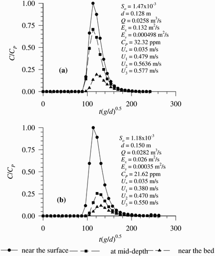
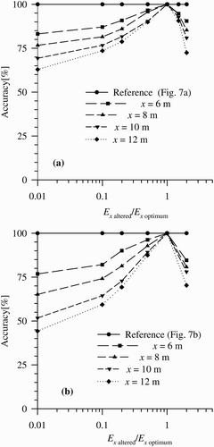
The sensitivity of the predicted C–t curves to the possible presence of errors in E _x and E _y was also checked and illustrated here using two data sets. The dimensionless (with reference to peak concentration at y/d = 1.0) C–t curves at three elevations along the vertical, i.e. at y/d = 0, 0.5 and 1.0, are shown in Fig. 7. Using the numerical scheme proposed by Singh et al. (2009), C–t curves were predicted at the various downstream sections using the observed optimum value of E _x and E _y . The corresponding C–t curves were also computed for altered values of E _x , with E _x varied by multiplying E _x by 0.01, 0.1, 0.2, 0.5, 1.5 and 2, respectively. These ERR values were compared with the ERR values corresponding to the optimum value of E _x . The accuracy of prediction of the C–t curves was then defined as (100−ERR). These values are plotted against the corresponding E _{x altered}/E _{x optimum} to illustrate the two data sets (Fig. 8). The accuracy for the predicted C–t curves reduced to about 70% if the value of E _x was altered by multiplication factors ranging from 0.2 to 2. However, the computed C–t curves were much less accurate if E _x was altered beyond these limits.

Figure 7 Input C–t curves used for sensitivity analysis of E _x and E _y

Figure 8 Effect of error in values of E _x on accuracy of predicted C–t curves

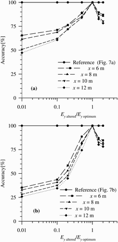
A similar analysis for E _y revealed that the accuracy for computing the C–t curve reduced to up to 70–50%, if the observed value of E _y is altered by multiplying it with factors ranging from 0.5 to 2, as illustrated in Fig. 9 for the same data set. Considerably less accurate results are produced if the E _y values were altered beyond these limits. Figures 8(a) and 9(a) pertain to the data set of Fig. 7(a), while Figs 8(b) and 9(b) correspond to the data set of Fig. 7(b). In both cases, if E _x and E _y are altered using multiplication factors ranging from 0.5 to 2, the peak concentration is only changed by about 10%. For E _x altered, the spread of the C–t curves increased about the peak while the peak value of pollutant concentration reduced. The higher values of E _x were associated with more spreading of the C–t curves and a larger decrease in the peak concentration. However, for high values of E _y , mixing in the vertical direction is rapid.

Figure 9 Effect of error in E _y on accuracy of predicted C–t curves

The likely errors in estimations of the mixing coefficient may originate from a complex channel geometry or buoyancy effects of pollutants. However, based on the sensitivity of the mixing coefficients, it was deduced that the errors that may likely occur in the estimation of E _x and E _y would result in a small error in the prediction of the C–t curves at channel sections downstream of the injection station. The sensitivity analysis indicated that the predictions of C–t curves can be made with a maximum error of about ±30% if about ±100% error is contained in E _x and E _y . On the basis of this analysis, it is therefore concluded that the optimum values of E _y derived by the numerical scheme compare well with the values determined based on the velocity distribution as the scatter among them is smaller than 2 times to about 1/2 times.

7 Conclusions

Laboratory experiments on passive mixing of pollutants in open channels with transverse line slug source on the flow surface were conducted. The finite difference scheme recently proposed by the authors for the prediction of pollutant concentration was extended to determine the optimum (observed) values of the mixing coefficients from the observed concentration versus time curves. The computed vertical mixing coefficient from an empirical equation and from the measured velocity distribution were compared with the optimum using the data of the present study and these collected from the literature. In both cases, most of the computed values lie within a scatter band of 50–100% times of the observed data. The errors, likely to occur in the predictions of the concentration versus time curves due to the use of the erroneous values of longitudinal and vertical mixing are quantified, indicating that the predictions of concentration versus time curves can be made with a maximum error of about ±30% if about ±100% error is contained in the values of longitudinal and vertical mixing coefficients. Based on the computational results, a constant longitudinal mixing coefficient equal to longitudinal dispersion coefficient of a 1D dispersion process is recommended for practice, rather than a variable value along the flow depth.

Notation

A(k)	=	area of observed C–t curves, k
b k	=	width of sub-area k
B	=	width of channel
C	=	width-averaged pollutant concentration
C P	=	peak concentration
C–t	=	concentration versus time
d	=	flow depth
d k	=	depth of sub area k
ERS	=	error in C–t curve
ERR	=	average error in C–t curve
E x	=	longitudinal mixing coefficient
E y	=	vertical mixing coefficient
k	=	index number
M	=	mass of tracer recovered at a section
N 1	=	total number of sub-areas
Q	=	discharge
R b	=	hydraulic radius corresponding to bottom
S o	=	bottom slope of channel
t	=	time
U k	=	width-averaged velocity over sub-area k
U	=	width-averaged longitudinal velocity
U *	=	shear velocity
U 1	=	width-averaged longitudinal velocity at flow surface
U 2	=	width-averaged longitudinal velocity at mid flow depth
U 3	=	width-averaged longitudinal velocity near bed
x	=	coordinate in longitudinal direction
y	=	coordinate in vertical direction

References

- Ahmad , Z. and Kothyari , U. C. 2001 . Time-line cubic spline interpolation scheme for solution of advection equation . J. Comput. Fluids , 30 ( 6 ) : 737 – 752 .
- Ahmad , Z. , Kothyari , U. C. and Ranga Raju , K. G. 1999a . Longitudinal dispersion in open channel flows . J. Hydraul. Eng. , 5 ( 2 ) : 1 – 21 .
- Ahmad , Z. , Kothyari , U. C. and Ranga Raju , K. G. 1999b . Finite difference scheme for longitudinal dispersion . J. Hydraulic Res. , 37 ( 3 ) : 389 – 406 .
- Einstein , H. A. 1942 . Formulas for the transportation of bed load . Trans. ASCE , 107 : 561 – 597 .
- Elder , J. W. 1959 . The dispersion of marked fluid particles in turbulent shear flow . J. Fluid Mech. , 5 ( 4 ) : 544 – 560 .
- Fischer , H. B. 1968 . Dispersion predictions in natural streams . J. Sanit. Eng. Div. ASCE , 94 ( SA5 ) : 927 – 944 .
- Fischer , H. B. , List , E. J. , Koh , R. C.Y. , Imberger , J. and Brooks , N. H. 1979 . Mixing in inland and coastal waters , New York : Academic Press .
- French , R. H. 1979 . Transfer coefficients in stratified channel flow . J. Hydraul. Div. ASCE , 105 ( 9 ) : 1087 – 1101 .
- Garde , R. J. and Ranga Raju , K. G. 2006 . Mechanics of sediment transportation and alluvial stream problems , New Delhi, , India : Wiley Eastern Limited .
- Guan , Y. , Altinakar , M. S. and Krishnappan , B. G. Two-dimensional simulation of advection-dispersion in open channel flows . Proc. 5th Intl. Conf. Cardiff, UK. Hydroinformatics , pp. 226 – 231 .
- Jobson , H. E. and Sayre , W. W. 1970a . Predicting concentration profiles in open channels . J. Hydraul. Div. ASCE , 96 ( 10 ) : 1983 – 1996 .
- Jobson , H. E. and Sayre , W. W. 1970b . Vertical transfer in open channel flow . J. Hydraul. Div. ASCE , 96 ( 3 ) : 703 – 724 .
- Khan , I. M. , Simons , R. R. and Gras , A. J. 2007 . Vertical diffusion of pollution from line source near a wall . J. Hydraulic Res. , 45 ( 3 ) : 365 – 369 .
- Kim , D. G. and Seo , I. W. 2000 . Modeling the mixing of heated water discharged from a submerged multiport diffuser . J. Hydraul. Eng. , 38 ( 4 ) : 259 – 270 .
- Lipsett , A. W. and Beltaos , S. 1978 . “ Tributary mixing characteristics using water quality parameters ” . Edmonton, CA : Alberta Research Council . Report SWE-78/04
- McNulty , A. J. 1983 . “ Dispersion of a continuous pollutants source in open channel flow ” . Christchurch, NZ : University of Canterbury . PhD thesis
- McNulty , A. J. and Wood , I. R. 1984 . A new approach to predicting the dispersion of a continuous pollutant source . J. Hydraulic Res. , 22 ( 1 ) : 23 – 34 .
- Nokes , R. I. 1986 . “ Problems in turbulent dispersion ” . Christchurch, NZ : University of Canterbury . PhD thesis
- Nokes , R. I. and Wood , I. R. 1988 . Vertical and lateral turbulent dispersion: Some experimental results . J. Fluid Mech. , 187 : 373 – 394 .
- Nokes , R. I. , McNulty , A. J. and Wood , I. R. 1984 . Turbulent dispersion from a steady two-dimensional horizontal source . J. Fluid Mech. , 149 : 147 – 159 .
- Rutherford , J. C. 1994 . River mixing , New York : John Wiley and Sons .
- Schiller , E. J. and Sayre , W. W. 1973 . “ Vertical mixing of heated effluents in open channel flow ” . Iowa City, , USA : Report No. 148. IIHR. University of Iowa .
- Schiller , E. J. and Sayre , W. W. 1975 . Vertical temperature profiles in open channel flow . J. Hydraul. Div. ASCE , 101 ( 6 ) : 749 – 761 .
- Seo , I. W. , Baek , K. O. and Jeon , T. M. 2006 . Analysis of transverse mixing in natural streams under slug tests . J. Hydraulic Res. , 44 ( 3 ) : 350 – 362 .
- Seo , W. , Lee , M. E. and Baek , K. O. 2008 . 2D modeling of heterogeneous dispersion in meandering channels . J. Hydraul. Eng. , 124 ( 2 ) : 196 – 204 .
- Shiono , K. , Scott , C. F. and Kearney , D. 2003 . Predictions of solute transport in a compound channel using turbulence models . J. Hydraulic Res. , 41 ( 3 ) : 247 – 258 .
- Singh , S. 2005 . “ Two-dimensional mixing of conservative pollutants in open channels ” . Patiala, , India : Thapar Institute of Engineering & Technology . PhD thesis
- Singh , S. , Ahmad , Z. and Kothyari , U. C. 2009 . Two-dimensional mixing of pollutants in streams with transverse line slug source . J. Hydraulic Res. , 47 ( 1 ) : 90 – 99 .
- Stefanovic , D. L. and Stefan , H. 2001 . Accurate two-dimensional solution of advection-diffusive-reactive transport . J. Hydraul. Eng. , 127 ( 9 ) : 728 – 737 .
- Tsai , T. L. , Yang , J. C. and Huang , L. H. 2002 . Hybrid finite-difference scheme for solving the dispersion equation . J. Hydraul. Eng. , 128 ( 1 ) : 78 – 86 .