On the Reynolds number sensitivity of smoothed particle hydrodynamics

ABSTRACT

This work investigates the Reynolds number sensitivity of the weakly compressible smoothed particle hydrodynamics method. A mode of instability previously reported for Poiseuille flow is systematically analysed for six relevant test cases. We discuss the influence of the presence of physical viscosity, investigate the origin of the instability for the Couette flow example and explore its implications on convergence properties. Moreover, a novel instability of slightly different nature, which arises in pipe flow with expanding diameter, is detected and a qualitative explanation is given. Since both types of instabilities also occur at Reynolds numbers well below the critical value, its origin is seen in high-frequency particle oscillations independent of any effects of turbulence. We further demonstrate for a flow over a sill and a weir that if there is no breakup of the fluid structure at low Reynolds numbers, then energy balance is accurately simulated even at high Reynolds numbers. Finally, the implications of the instability are addressed from a theoretical, computational and practical perspective.

Keywords:

• Lagrangian particle methods
• low-Reynolds-number flows
• smoothed particle hydrodynamics model
• transition to turbulence
• two-dimensional numerical simulation

View correction statement:

Corrigendum

1 Introduction

In 1977 Gingold and Monaghan and Lucy introduced the fully Lagrangian meshless smoothed particle hydrodynamics (SPH) method to solve astrophysical problems like star or galaxy formation. Since then SPH has been applied to a wide range of problems, predominantly in fluid mechanics, from free surface flows (Monaghan 1994; Ferrari 2010; Gomez-Gesteira et al. 2010) to multiphase problems (Colagrossi and Landrini 2003; Aristodemo et al. 2010) and transport phenomena (Tartakovsky et al. 2007). The principle of SPH is to discretize the fluid into particles, which are moved according to a kernel-smoothed influence of its neighbourhood. Consequently, particle interactions are governed by discrete equations, in which derivatives of field variables are expressed in terms of smoothing kernel gradients. The Lagrangian nature of the method allows for exact treatment of advection and conservation of mass, momentum and energy (Price 2011). Additionally, free surfaces are implicitly supported (Monaghan 1994) and its tracking is simple (Shao and Gotoh 2005). In comparison with conventional computational fluid dynamics methods, however, implementation of inflow and outflow boundaries is complex and simulations are computationally expensive due to continuous neighbourhood search. Hence, numerical tests are frequently carried out in two dimensions even though the step to 3D is in theory straightforward (Ferrari et al. 2009).

Depending on the application, the fluid incompressibility criterion can be relaxed which subsequently leads to a reduction of the computational cost. The reason is that incompressible smoothed particle hydrodynamics (ICSPH) accounts for truly incompressible fluids, but requires the computationally expensive solving of a pressure Poisson equation. In the weakly compressible approach (WCSPH), however, the relation between pressure and density is given by an inexpensive equation of state (Monaghan 1994). This strategy allows for small density variations (Morris et al. 1997) and hence pressure fluctuations occur in the numerical solution. Whereas both methods yield comparable results in dam-break simulations (Hughes and Graham 2010), a recent comparative study concludes that WCSPH with a corrective algorithm is slightly more attractive in terms of accuracy, stability and computational demand than ICSPH (Chen et al. 2013).

Fluid flow either occurs in laminar or turbulent regimes, depending on whether the Reynolds number is below or above a critical value. In the former case, the dynamics are characterized by parallel moving layers, though in the latter case effects of randomness become important. The definition of the Reynolds number for two-dimensional pipe flow is , where D, and ν are pipe diameter, average velocity and kinematic viscosity. While D and are determined by the geometry and the external forces of the problem, ν varies significantly depending on the fluid type. Due to the reciprocal relationship between Reynolds number and viscosity, the dynamics of a certain type of flow are subject to earlier transitions to a turbulent regime if the fluid viscosity is reduced. Since SPH simulations are stabilized by a fluid's physical viscosity, it is challenging to simulate low viscous flows.

Therefore, SPH Poiseuille and Couette flow simulations have mainly been carried out in high viscous settings. Results are in good agreement with analytical solutions (Watkins et al. 1996; Morris et al. 1997; Adami et al. 2012) and are thus frequently used for benchmarking no-slip wall conditions. Typically chosen parameters are a viscosity and a maximum Reynolds number of 5, which supports the stability of the simulation. The concept of this work is inspired by deteriorations in the numerical solution for pipe and channel flow that occur if viscosity is reduced to the value of water. Even though this is of importance for practical applications, corresponding Poiseuille flow has rarely been studied and only at low (Morris et al. 1997, ) or moderate (Sigalotti et al. 2003, R=5) Reynolds numbers. While in high viscous specifications transient velocity profiles are known to coincide with analytical solutions up to a Reynolds number of about 10³, exact localization of the critical value, where the transition from laminar to turbulent flow begins, is subject to ongoing work – in particular for low physical viscosity. Hence, the primary aim of this work is to explore the sensitivity of the SPH method on the Reynolds number. Therefore, we systematically study six relevant test cases and explore a mode of instability, which depends on and grows with the Reynolds number. Since this instability also occurs well below the critical Reynolds number, its origin is not seen in effects of turbulence but in high-frequency particle oscillations.

We begin by studying a Poiseuille flow to demonstrate the Reynolds number dependency of the weakly compressible SPH method. It is shown that good accuracy and convergence properties are found for low Reynolds number transient and steady solutions, but once a certain threshold is exceeded the accuracy of the simulation significantly drops due to the numerical breakup of the fluid structure. Therefore, we explore the origin of the instability, which is shown to depend on and increase with the Reynolds number. The novelty in comparison with previous work (Sigalotti et al. 2003; Basa et al. 2009) is seen in a more detailed discussion which, e.g. firstly demonstrates the analogy of the instability for the Couette flow example and also explores the difficulties that arise in the presence of a low physical viscosity. Moreover, a novel mode of instability, which occurs in pipe flow with expanding diameter, is presented and a qualitative explanation for its initiation is given. We further address the implications of the observed stability problems to open channel flow applications. In particular, it is shown that for low viscous free surface flows with an initially uniform particle distribution the simulated velocity profile deviates shortly after imposing the analytical solution. The second section of the paper is then devoted to demonstrating two examples which are not affected by the mode of instability: It is shown that for flow over a sill and a sharp-crested weir energy balance based on Bernoulli's principle is accounted for correctly even at high Reynolds numbers. In the final section the relevance of the instability is addressed from a theoretical, computational and practical point of view.

2 Method

The fundamental principle of SPH is to discretize the fluid into interpolation points which are interpreted as particles such that their coordinates move along with the fluid. Initially, these particles are arranged on a rectangular grid with a uniform sampling distance sd and associated with mass m, volume V, velocity vector , density ρ and pressure p. The mass is kept constant, but other physical variables are governed by discrete SPH equations derived through interpolation of the continuum equations of fluid dynamics. Owing to the symmetries in the corresponding Hamiltonian, conservation of energy as well as of linear and angular momentum is inherent. Through time integration of the governing equations, the evolution of a particle's physical parameters is determined by a weighted influence of its neighbourhood. Since we aim at testing the capabilities of standard weakly compressible SPH, no turbulence model is used and only essential enhancements like the density reinitialization are applied.

2.1 Governing equations

Characteristic of SPH is the weighting by a smoothing kernel , where denotes the position vector in space and identifies the smoothing length. There is a freedom in the choice of the kernel, but symmetry, partition of unity and convergence to the δ-function in the limit of vanishing smoothing length are required. Due to high computational accuracy (Hongbin and Xin 2005), we use the Quintic spline with a compact support of three neighbours:

This Quintic kernel is expressed in terms of the dimensionless variable and normalized for two dimensions. Disadvantages of the Quintic spline include significant computational cost owing to its piecewise definition and the appearance of the pairing instability (Dehnen and Aly 2012).

For derivation of the equations of motion see, e.g. (Monaghan 1988; Gomez-Gesteira et al. 2010). We choose the following discrete representation of the continuity equation to ensure that the null pressure condition at free surfaces is implicitly satisfied (Bonet and Lok 1999):

with the abbreviations and . Technically, the sum over the index j involves all fluids except for particle i. Due to the chosen kernel width, however, only the three adjacent neighbours of i have a non-vanishing contribution. The momentum equation, which controls a particle's acceleration, has pressure, artificial viscosity and shear forces contributions:

The variable ν corresponds to the physical viscosity, weighted density and pressure are abbreviated as and . Note that the antisymmetry of Eq. (3) is required to ensure conservation of linear momentum. Artificial viscosity, as defined in Section 2.3, is added to stabilize the method. To close the set of equations we further require a relation between pressure and density, which is given by the equation of state (WCSPH, Monaghan 1994)

Thereby the reference density is equal to the initial fluid density and the sound speed is set to . Hence, it can be shown by a scale analysis that maximum density fluctuations are limited to 1% (Morris et al. 1997).

2.2 Velocity-verlet integration

We use the second-order velocity-Verlet integration as a time-stepping scheme

which is sensible in terms of computational cost as a particle's acceleration only has to be calculated once per time-step. The size of Δ t is determined by the flow velocity, viscosity and gravitational acceleration:

2.3 Artificial viscosity

In WCSPH artificial viscosity is required to stabilize the method (for an overview see González et al. 2009). The following term, which gives rise to a physical kinematic viscosity , is applied between fluid particles (Monaghan and Gingold 1983):

This formulation reduces irregular unphysical motion, but requires a tuning parameter in the range of . If the influence of artificial viscosity becomes comparable to physical viscosity, it can modify the global solution. Particularly in low viscous settings it is challenging to dampen small fluctuations whilst otherwise not affecting the simulation.

A further drawback of weakly compressible SPH oscillations spurious pressure are which can be cured with low additional computational cost by applying a Shepard filter. In doing so the kernel is corrected at zeroth-order and consequently the fluid density is reinitialized every 25 time-steps according to (Monaghan and Gingold 1983)

2.4 Boundary conditions

Two different strategies are followed to model solid boundaries with SPH. One approach is to correct the SPH equations with an Eulerian renormalization term which depends on the shape of the wall. Alternatively, solid boundaries are represented by fixed wall particles, where the interaction is either modelled by an unphysical Lennard-Jones-like potential or an expensive creation of mirror particles at each time-step. We use a conceptually simple and adaptive modification based on imposing a local force balance between fluid and fixed wall particles (Adami et al. 2012).

With this method wall particles are not evolved according to the governing equations, but the influence of its physical parameters is included in the continuity and momentum equations. Hence, three layers of solid particles are required to ensure full kernel support. A virtual wall particle velocity is determined by an antisymmetric extrapolation from adjacent fluid particles

and its incorporation in the shear forces contribution in Eq. (3) imposes a no-slip condition at the wall. The prescribed velocity is set to zero except for moving boundaries. Local force balance gives rise to a wall particle's pressure of

so that fluid particles are repelled as they approach the solid boundary. Density is then assigned by the inverted equation of state

For the modelling of in- and outflow boundaries, depending on the characteristics of the test case we either impose periodic boundaries or use buffer zones for insertion and removal of particles. The former boundary conditions are achieved my mirroring the kernel from the inflow to the outflow section and vice versa. We refer to Federico et al. (2012) for a detailed description of the buffer zone technique.

3 Two-dimensional test cases

In Sections 3.1 and 3.2 the WCSPH model is applied to two-dimensional pipe and open channel flow to explore the Reynolds number sensitivity of the method. Thereby, we closely explore a mode of instability previously reported by other authors for Poiseuille flow (Sigalotti et al. 2003; Basa et al. 2009). Apart from firstly demonstrating an analogue behaviour in the Couette flow example, we investigate the influence of the amount of physical viscosity being present. Hereafter, the use of the term low viscosity refers to a kinematic viscosity parameter of , which approximates the value of water at a temperature of 20 °C. Contrary, high viscous settings indicate a viscosity of . We further detect and qualitatively explain a novel mode of instability for pipe flow with expanding diameter, which is shown to depend on the geometric specifications of the problem. At the end of this work, it is then demonstrated that energy balance of flow over a sill and over a sharp-crested weir is satisfied at high Reynolds numbers without any deteriorations in case of low physical viscosity. Thereby, it becomes clear that the occurrence of the instability is restricted to certain geometries.

3.1 Pipe flow

The first set of test cases represents flows within closed conduits. Except for example 3, we simulate a section of small width such that L_x=L_y and impose periodic boundaries on the edges (c.f. Fig. 1, solid lines). No-slip boundary conditions are prescribed on the solid walls.

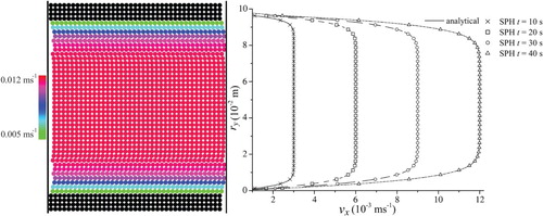
Figure 1. Poiseuille flow particle distribution (left) and velocity profile (right) (t=40 s, R=1050)

3.1 Poiseuille flow

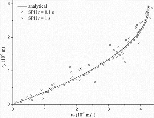
External force-driven flow between two plates is referred to as Poiseuille flow. Whilst fully developed Poiseuille flow with high viscosity was simulated with SPH (Watkins et al. 1996; Ferrand et al. 2012), stabilization of low Reynolds number Poiseuille flow requires an adapted formulation of viscosity based on an estimation of viscous diffusion to maintain accurate velocity profiles (Morris et al. 1997). Since we find that also the velocity profile of moderate Reynolds number Poiseuille flow is disturbed by artificial viscosity, this procedure is not applied. For low viscous Poiseuille flow with a plate distance of , the results agree with the series solution for 52 s after an external acceleration parallel to the plates of strength commenced. In Fig. 1 layer-wise moving particles are depicted and the SPH velocity profile measured at the centre of the simulated section is compared with the analytical solution. At t=40 s the agreement is within and improves to by doubling the number of particles. The convergence rate is 1.9, slightly below the theoretical order 2 of the velocity-Verlet scheme. Identical convergence is obtained for high viscous Poiseuille flow (Adami et al. 2012; Ferrand et al. 2012). Comparable convergence properties are found for transient states up to t=40 s, although the rate of convergence drops at later times due to the initiating transition to turbulent flow.

To explore the Reynolds number dependency of the simulation more closely, a series of Poiseuille flow studies with varying body forces is performed. The sound speed is set to 10 times the maximum flow velocity of the steady state. If instabilities lead to programme abortion before obtaining a steady solution, 10 times the flow speed prior to abortion is used. We achieve steady states, where driving and friction forces are in balance, for flows up to a Reynolds number of 62.5. The agreement is within 0.5 % for , but reduces to 8.2 % as the threshold is approached. If the Reynolds numbers are further increased, however, the laminar fluid structure, i.e. parallel layer-wise moving particles, breaks and thus we do not attain any steady state. The higher the Reynolds number, the earlier the particle distribution differs from a laminar state. The results in Table 1 confirm that transient laminar distributions are achieved up to , but suggest that steady laminar states are only obtained for R<65. In particular, we find that due to low viscous forces the velocity of each particle layer fluctuates around the analytical solution. Owing to particle interactions, neighbouring rows alternately have a too high or low velocity. Hence, if a particle gets marginally vertically displaced, it swings past a neighbouring particle of the next layer (Basa et al. 2009) such that small eddies develop which spoil the laminar fluid structure. The effect can be reduced by adding artificial viscosity. However, this is avoided to maintain accurate velocity profiles. If the particle movement is constricted to the direction parallel to the plates, vertical oscillations are suppressed and hence the stability threshold is deferred to higher Reynolds numbers.

Table 1.  Poiseuille flow simulation characteristics with 39 particles across the diameter (v = 10^-6 m² s^-1)

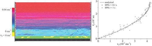
3.1 Couette flow

Since previous work only reported the mode of instability for Poiseuille flow (Sigalotti et al. 2003; Basa et al. 2009), it is important to investigate if the unstable behaviour is specific to this test case or whether it appears more generally. For the slightly modified Couette flow example (c.f. Fig. 2), which is driven by an upper wall of constant velocity , we expect similar stability properties as for Poiseuille flow. With the same geometric specifications as before and a sound speed of 10 times the upper wall velocity, the simulation is stable for 30 s. Up to this time the error in reference to the series solution and the order of convergence are comparable to the Poiseuille flow results.

Figure 2. Couette flow velocity profile

We now locate the Reynolds number threshold, where steady states are achieved, by varying the upper wall velocity. At large times and for Reynolds numbers above 25, the top and bottom fluid layers approach the plates. Consequently, neighbouring layers arrange pairwise and thus the accuracy is reduced. Once a threshold of R>70 is crossed, the layer-wise moving structure breaks and thus the programme aborts before pairwise arrangements occur (c.f. Table 2).

Table 2.  Couette flow simulation characteristics with 39 particles across the diameter (v = 10^-6 m²s^-1)

In summary, low viscous Poiseuille and Couette flow simulations have similar characteristics: steady solutions are found for R<65, but the agreement rapidly deteriorates as this threshold is approached. If the bulk velocity is further increased, the simulation aborts before steady particle distributions are obtained. Transient states, however, are simulated accurately. Since in the Couette flow the fluid is driven by a constant wall velocity, in proximity of the upper wall boundary neighbouring fluid particles of the same layer arrange pairwise. Consequently, deterioration and abortion of the simulation occurs slightly earlier than for Poiseuille flow.

3.1 Low viscous pipe flow with variable diameter

We replace the periodic boundaries by a continuous two-dimensional inflow of to simulate a frictionless pipe with a diameter of 1 m. Preliminary simulations indicate that the previously identified mode of instability does not occur in this example since the limited length restricts the buildup of particle fluctuations. In addition, the modified inflow algorithm is also expected to counteract the instability because particles do not arrange in a strict layer-wise structure. After modifying the pipe geometry, however, such that its middle segment narrows to before increasing to its initial height, a novel instability of different nature is discovered (c.f. Fig. 3a). The average simulated velocities at the centre of each segment are , and . Thus, the flow rates in areas A and B,

satisfy continuity of flow.

Figure 3. Particle and velocity distribution in a pipe with varying diameter at (a) high (R=1.4×10⁶) and (b) low (R=7×10⁻¹) Reynolds number for 50 particles along the pipe diameter and with an artificial viscosity parameter of α=2×10⁻²

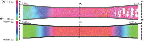
The fluid, however, is not decelerated in area C as it should when the pipe expands. As a consequence, an instability develops in the expanding section and eventually breaks the fluid structure. Increasing the artificial viscosity raises the coherence of particles, but it does not prevent the fluid structure from breaking. Interestingly, these stability problems are not encountered after reducing the inflow and length scales to obtain a decreased Reynolds number of . The simulation results presented in Fig. 3b indicate a uniform particle distribution and consequently continuity of flow is now satisfied in all areas:

To investigate the Reynolds number dependency of the instability and to find a qualitative explanation for the breakup of the fluid structure, we slowly increase the Reynolds number. No stability problems arise up to a Reynolds number of 100, but once this threshold is crossed the prior uniformly distributed particles arrange in pairwise lines in the expanding part of the pipe. At later times the neighbouring lines collide at the edges and repel each other in the centre (c.f. Fig. 4). As a consequence, a breakup of the fluid structure initiates from the centre of the pipe and eventually spreads throughout the expanding section. The propagation of the instability increases with higher Reynolds numbers.

Figure 4. Initiating breakup of the fluid structure in the expanding section of the pipe (R=100)

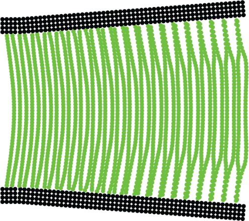
In conclusion, narrowing sections in a pipe are simulated accurately even at high Reynolds numbers. Without appropriate corrections, however, particles fail to rearrange uniformly as the pipe expands, which eventually results in the breakup of the fluid structure. This problem does not occur at Reynolds numbers below 100.

3.2 Open channel flow

In this section the implications of the discovered mode of instability are discussed on the basis of open channel flow simulations. If periodic boundaries are imposed at the edges, then the simplest open channel flow test case is to drive an initially stationary fluid by the component of the gravitational acceleration parallel to a channel bed of slope s₀. Apart from the additional force component orthogonal to the flow direction and the absence of an upper solid wall, the flow characteristics are similar to Poiseuille flow. Consequently, we a priori expect an instability even though fluid structure problems have not previously been reported in the literature for these type of flows.

The first part of this section is devoted to showing that in high viscous specifications the viscous force contributions are strong enough to stabilize the simulation such that the velocity profile converges to the correct values. If the simulation, however, is repeated after reducing the viscosity to the value of water, then the velocity distribution deviates shortly after imposing the analytical solution. In the second part we demonstrate on the basis of two subproblems of open channel flow, namely for flow over a sill and over a sharp-crested weir example, that energy balance is simulated correctly without any Reynolds number-dependent stability problems.

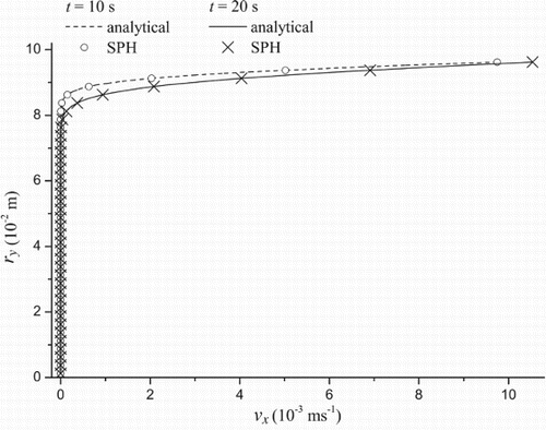
3.2 High viscous free surface channel flow

An initially stationary fluid block of height is driven by a bed slope s₀=10⁻³. Since abrupt initiation of gravitational forces would lead to spurious oscillations, the impact of the body force is deferred by a sine-like damping term for the first 3 s (Monaghan and Kajtar 2009). As for pipe flow artificial viscosity modifies the velocity profile and thus it is not applied. The simulation converges to a uniform laminar solution with a horizontal velocity distribution of (Graf and Altinakar 1998)

As the flow characteristics only depend on the vertical distance from the channel bed, the velocities are horizontally averaged. For the chosen resolution the velocity profile converges (c.f. Fig. 5) and the agreement is within 1%.

Figure 5. Converged velocity profile of laminar free surface channel flow for a resolution of 36 particles across the channel height (t=50 s, R=7.5×10⁻¹)

3.2 Low viscous free surface channel flow

The simulation is repeated in low viscous conditions with reduced geometric specifications such that . Despite varying both the channel slope parameter s₀ and the particle spacing, we could not reproduce the results achieved for high viscous channel flow. Due to the strong vertical component of the gravitational force, a small bed slope results in a dislocation of horizontal layers at early times. In particular, layers close to the bottom move with significantly different velocities – at times opposite to the direction of flow. A choice of higher bed slopes, which is significantly limited by demanding for laminar flow conditions, defers the experienced problems, but does not prevent the laminar structure from breaking. As neither increasing artificial viscosity nor adding a damping term improves the results, we substitute the initially stationary fluid block for its analytical solution and investigate stability.

Consequently, the damping term is removed. The horizontal velocity as determined by Eq. (14) and the corresponding pressure distribution are initially imposed. For a bed slope of s₀=10⁻⁵ Fig. 6 shows the particle distribution and compares the velocity profile to the analytical solution. The particle plot indicates that the layer-wise moving fluid structure breaks, several particles close to the bottom move opposite to the flow direction. As the simulation continues, the velocity profile clearly deviates from the analytical solution. These results indicate the difficulties in simulating steady laminar states for low viscous fluids like water with the standard formulation of SPH.

Figure 6. Open channel flow particle distribution (left, t=1.4 s, R=798 ) and deviation of the velocity profile (right) for a resolution of 59 particles across the channel height

3.2 Flow over a sill

To simulate a flow over a sill it is important to track deformed free surfaces and thus mesh-free particle methods are often preferred to Eulerian approaches (Sahebari et al. 2011). The special case of a hydraulic jump, i.e. the transition from super- to subcritical flow, is a standard SPH experiment (Lopez et al. 2010; Federico et al. 2012). Since distinctive backwater results in a discontinuous free surface level and hence causes significant losses, it is challenging to monitor energy balance. However, both the converse transition and supercritical flow are approximately loss-free and can be realized by placing a crested sill with a linear slope of in the centre of the channel.

Sub- to supercritical flow

The particle distribution of a low viscous flow over a crested sill with subcritical upstream and supercritical downstream conditions is shown in Fig. 7a. The simulated free surface levels and fluid velocities (c.f. Table 4) correspond to an upstream Froude number below 1, which increases to 1.12 downstream of the sill. Since the continuous water surface level implies negligible energy losses, the fluid is accelerated downstream of the sill such that the water level declines. By computing the downstream water surface level (subindex B) from the measured upstream quantities (subindex A), we find that energy balance is accounted for correctly:

Figure 7. Flow over a sill particle plot for (a) a transition from sub- to supercritical flow and (b) supercritical flow (α=5×10⁻², sd=2×10⁻² m)

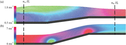
Table 3.  Inflow and geometric specifications for the flow over a sill problem

Flow	Inflow	Inflow	Sill	Sill
condition	velocity	height	height	width
		(m)
Sub- to supercritical		1		1.5
Supercritical	7			1.5

Table 4.  Simulated water surface levels and average fluid velocities for a flow over a sill with a transition from sub- to supercritical flow

Position relative to sill	F		H (m)
1 m upstream (A)
1 m downstream (B)	1.12	1.7

Supercritical flow

The inflow characteristics and the sill height are adapted as specified in Table 3. Thereby, the critical Froude number F=1 is exceeded up- and downstream the sill such that the flow conditions are supercritical throughout the channel. Conservation of energy implies a downstream free surface level of , which roughly agrees with the measured value (c.f. Table 5).

Table 5.  Simulated water surface levels and fluid velocities for a supercritical flow over a sill

position relative to sill	F		H (m)
1 m upstream (A)	4.09	7.01
1 m downstream (B)	3.44	6.29

In summary, high Reynolds number SPH simulations of a flow over a sill are in agreement with Bernoulli's principle. In case of the transition from sub- to supercritical flow the downstream water level rises, whereas it declines for supercritical flow. Accuracy is only marginally influenced by the choice of artificial viscosity. In contrast to previous test cases, we do not detect any stability problems at high Reynolds numbers.

3.2 Flow over a sharp-crested weir

In the final test case we investigate energy balance of a flow over a sharp-crested weir. Again, the aim is to show that high Reynolds number standard SPH simulations are stable and agree with Bernoulli's principle. The simulation characteristics are summarised in Table 6.

Table 6.  Simulation characteristics of the flow over a sharp-crested weir example

inflow			observation
velocity	sd (m)	α	period (s)
1			24.5−25

Frequently, Poleni's formula is chosen as reference solution

where denotes the weir head. Since in this formula the geometry of the weir is only incorporated by an empiric shape factor μ and the inflow velocity is neglected, we aim for a more sophisticated reference solution. If frictionless conditions are assumed, the differential flow rate can be expressed in terms of the parabolic velocity distribution. Integrating yields the total flow rate (Bollrich 2010)

The weir head and the average inflow velocity are measured upstream of the weir, M corresponds to the lowering rate of the overfall flow (c.f. Fig. 8a).

Figure 8. Velocity distribution of the flow over a sharp-crested weir with a convergence analysis of the overfall flow rate

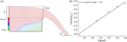
For the observed time period, Fig. 8b indicates convergence of the overfall flow rate with an order of 1.38 and hence at the highest resolution the computed rate is in good agreement with the analytical solution according to Eq. (17):

Consequently, energy balance of a flow over a sharp weir is simulated correctly even at high Reynolds numbers without any breakup of the fluid structure. The flow rates fluctuate around the analytical solution, but average quantities closely match the reference values. Whilst no stability problems arise in low viscous settings, the fluctuations of the flow rate reduce even further if the amount of physical viscosity is increased.

4 Relevance of the instability

At the end of this work we discuss the theoretical, computational and practical relevance of the instability. In summary, two different categories of instabilities are identified. The instability of the first type is attributed to the fundamental principle of the SPH method. If a certain Reynolds number threshold is exceeded, unphysical particle oscillations build up which eventually result in a breakup of the fluid structure. All test cases where this instability is observed have the similarities of an infinite problem domain and a regular layer-wise initial particle distribution. The second type of instability, however, depends on the geometry of the problem and is demonstrated with the example of pipe flow with expanding diameter.

Theoretical relevance. Due to its universal origin the instability of the first type is highly relevant from a theoretical perspective. Even though Basa et al. (2009) qualitatively explains the instability for the Poiseuille flow example, it is of future interest to rigorously analyse and understand its source. This is also the first step required to developing a corrective algorithm specifically devoted to curing this instability. Applying established non-specific particle shifting algorithms (Adami et al. 2013) or coarsely constricting the oscillatory particle movement may defer but not prevent the breakup of the fluid structure. In comparison, it is simpler to understand and cope with the instability of the second type. The associated fluid structure problems, however, are less relevant from a theoretical perspective since its occurrence is associated with specific geometries.

Computational relevance. An understanding of both instabilities is particularly important to limit the computational demand. The absence of any criterion for programme abortion causes a significant computational overhead since the simulation continues over long times despite obviously inadequate results. In the Poiseuille flow example the simulation characteristics presented in Table 1 indicate that the transition time between the initiation of the instability and the final breakup can be long. Hence, we recommend to monitor the distance between particles of the same layer to detect the instability of the first type at early times. The transition time of the instability of the second type is much shorter such that void zones develop shortly after its initiation. These regions are easily identifiable in graphical outputs or by monitoring the number of neighbours of each particle.

Practical relevance. In this work the Reynolds number sensitivity of the SPH method is explored for several subproblems, which if assembled may constitute a practical application. Hence, a rough assessment on the robustness of a more complex application can be made by dividing the set-up into a number of subproblems whose stability properties are known. As indicated at the beginning of this section the instability of the first type only occurs in infinite domains with an initially regular particle configuration. These conditions are rarely fulfilled in practical applications since particles do not arrange in strict layers which limits the buildup of unphysical particle oscillations. If the geometry of the problem stimulates the instability of the second type, a corrective algorithm is required to obtain meaningful results. With respect to the determined Reynolds number threshold, it has to be pointed out that due to the low physical viscosity this critical value is exceeded in the majority of applications which include water as liquid phase. In consequence, steady-state laminar flow conditions cannot be obtained with the standard formulation of SPH except for very small Reynolds numbers.

5 Conclusions

Weakly compressible SPH without any turbulence model was systematically applied to six relevant test cases to explore the method's sensitivity on the Reynolds number. It is shown that the accuracy of SPH pipe and channel flow simulations strongly depends on the physical viscosity being present and correspondingly on the Reynolds number governing the flow. In high viscous settings accurate pipe flow results are obtained up to the critical Reynolds number threshold where the transition of the flow to a turbulent regime begins. In low viscous settings, however, unphysical particle fluctuations occur and rise with the Reynolds number. Once a threshold value of about 65 is exceeded, i.e. effects of turbulence can be ruled out, the particle fluctuations build up and lead to programme abortion before a steady solution is attained. It is further demonstrated that a mode of instability with similar characteristics arises in open channel flow simulations of infinite length. In pipe flow with varying diameter a novel Reynolds number dependent mode of instability is detected. This instability is shown to be sensitive to the geometry of the problem such that it only occurs in expanding sections of the pipe. Neighbouring lines of particles collide at the edges and repel each other in the centre, which eventually initiates a breakup of the fluid structure from the centre of the pipe.

To confine the area of influence of the instabilities, it is shown that two subproblems of open channel flow, namely a flow over a sill and a weir, are not affected by the mode of instability. The key difference to previous test cases is that the periodic boundaries are substituted by inflow buffer zones such that the problem domains are of finite length and the initial particle configuration is unregular. Because both requirements are usually satisfied in real applications, from a practical perspective the instability of the second type is of higher relevance. Since the origins of the instability of the first type are attributed to the fundamental principle of the SPH method, the associated structure problems are theoretically and computationally relevant. From the theoretical viewpoint the future work remains to develop an algorithm that cures the origins of the instability. Regarding computational effectiveness, we recommend to monitor the inter-particle distances to deliberately abort the simulation if the instability initiates.

Funding

This research is part of a project that is funded by the Austrian Science Fund (FWF): [P26768-N28].

Notation

=	=	body force acceleration ()
α =	=	artificial viscosity strengthness parameter (−)
c =	=	sound speed ()
D =	=	pipe diameter (m)
=	=	external force ()
F =	=	Froude number (−)
=	=	gravitational acceleration ()
h =	=	smoothing length (m)
=	=	weir head (m)
H =	=	water surface level (m)
Lx =	=	length of a channel (m)
Ly =	=	width of a channel (m)
m =	=	mass (kg)
M =	=	lowering rate of overfall flow (−)
μ =	=	shape factor in Poleni's formula (−)
p =	=	pressure (Pa)
ρ0 =	=	reference density ()
ρi =	=	density of particle i ()
q =	=	dimensionless kernel distance (−)
Q =	=	total 2D flow rate ()
=	=	position vector in space (m)
rx =	=	x-coordinate of the position vector (m)
ry =	=	y-coordinate of the position vector (m)
R =	=	Reynolds number (−)
sd =	=	particle spacing (m)
s0 =	=	channel bed slope (−)
t =	=	elapsed simulation time (s)
=	=	time until simulation aborts (s)
=	=	simulation time until steady state is reached (s)
Δ t =	=	time increment (s)
=	=	fluid velocity ()
=	=	average velocity upstream of overfall flow ()
=	=	velocity of particle i ()
=	=	prescribed velocity of wall particles ()
vx =	=	x-coordinate of the velocity vector ()
vy =	=	y-coordinate of the velocity vector ()
Vi =	=	volume of particle i(m3)
ν =	=	kinematic viscosity ()
W =	=	smoothing kernel (m−2)
Δ x =	=	difference in horizontal position (m)
Δ y =	=	difference in vertical position (m)
f =	=	fluid particle index
i =	=	reference particle index
j =	=	neighbouring particle index
w =	=	wall particle index

References

- Adami, S., Hu, X., Adams, N. (2012). A generalized wall boundary condition for smoothed particle hydrodynamics. J. Comput. Phys. 231, 7057–7075. doi: 10.1016/j.jcp.2012.05.005
- Adami, S., Hu, X., Adams, N. (2013). A transport-velocity formulation for smoothed particle hydrodynamics. J. Comput. Phys. 241, 292–307. doi: 10.1016/j.jcp.2013.01.043
- Aristodemo, F., Federico, I., Veltri, P., Panizzo, A. (2010). Two-phase SPH modelling of advective diffusion processes. Environ. Fluid Mech. 10, 451–470. doi: 10.1007/s10652-010-9166-z
- Basa, M., Quinlan, N., Lastiwka, M. (2009). Robustness and accuracy of SPH formulations for viscous flow. Int. J. Numer. Meth. Fluids 60, 1127–1148. doi: 10.1002/fld.1927
- Bollrich, G. (2010). Technische Hydromechanik 1. Verlag Bauwesen, Berlin.
- Bonet, J., Lok, T. (1999). Variational and momentum preservation aspects of SPH formulations. Comput. Meth. Appl. Mech. Eng. 180, 97–115. doi: 10.1016/S0045-7825(99)00051-1
- Chen, Z., Zong, Z., Liu, M., Li, H. (2013). A comparative study of truly incompressible and weakly compressible SPH methods for free surface incompressible flows. Int. J. Numer. Meth. Fluids 73, 813–829. doi: 10.1002/fld.3803
- Colagrossi, A., Landrini, M. (2003). Numerical simulation of interfacial flows by smoothed particle hydrodynamics. J. Comput. Phys. 191, 448–475. doi: 10.1016/S0021-9991(03)00324-3
- Dehnen, W., Aly, H. (2012). Improving convergence in smoothed particle hydrodynamics simulations without pairing instability. Mon. Not. R. Astron. Soc. 425, 1068–1082. doi: 10.1111/j.1365-2966.2012.21439.x
- Federico, I., Marrone, S., Colagrossi, A., Aristodemo, F., Antuono, M. (2012). Simulating 2D open-channel flows through an SPH model. Eur. J. Mech. B – Fluids 34, 35–46. doi: 10.1016/j.euromechflu.2012.02.002
- Ferrand, M., Laurence, D., Rogers, B., Violeau, D., Kassiotis, C. (2012). Unified semi-analytical wall boundary conditions for inviscid, laminar or turbulent flows in the meshless SPH method. Int. J. Numer. Meth. Fluids 71, 446–472. doi: 10.1002/fld.3666
- Ferrari, A. (2010). SPH simulation of free surface flow over a sharp-crested weir. Adv. Water Resour. 33, 270–276. doi: 10.1016/j.advwatres.2009.12.005
- Ferrari, A., Dumbser, M., Toro, E., Armanini, A. (2009). A new 3D SPH scheme for free surface flows. Comput. Fluids 38, 1203–1217. doi: 10.1016/j.compfluid.2008.11.012
- Gingold, R., Monaghan, J. (1977). Smoothed particle hydrodynamics – theory and application to non-spherical stars. Mon. Not. R. Astron. Soc. 181, 375–389. doi: 10.1093/mnras/181.3.375
- Gomez-Gesteira, M., Rogers, B., Dalrymple, R., Crespo, A. (2010). State-of-the-art of classical SPH for free-surface flows. J. Hydraulic Res. 48, 6–27. doi: 10.1080/00221686.2010.9641242
- González, L., Sánchez, J., Macià, F., Souto-Iglesias, A. (2009). Analysis of WCSPH laminar viscosity models. Proc. Int. Conf. SPHERIC SPH Workshop, Nantes, 179–186.
- Graf, W., Altinakar, M. (1998). Fluvial hydraulics: Flow and transport processes in channels of simple geometry. John Wiley and Sons, Bognor Regis.
- Hongbin, J., Xin, D. (2005). On criterions for smoothed particle hydrodynamics kernels in stable field. J. Comput. Phys. 202, 699–709. doi: 10.1016/j.jcp.2004.08.002
- Hughes, J., Graham, D. (2010). Comparison of incompressible and weakly-compressible SPH models for free-surface water flows. J. Hydraulic Res. 48, 105–117. doi: 10.1080/00221686.2010.9641251
- Lopez, D., Marivela, R., Garrote, L. (2010). Smoothed particle hydrodynamics model applied to hydraulic structures: A hydraulic jump test case. J. Hydraulic Res. 48, 142–158. doi: 10.1080/00221686.2010.9641255
- Lucy, L. (1977). A numerical approach to the testing of the fission hypothesis. Astron. J. 82, 1013–1024. doi: 10.1086/112164
- Monaghan, J. (1988). An introduction to SPH. Comput. Phys. Commun. 48, 89–96. doi: 10.1016/0010-4655(88)90026-4
- Monaghan, J. (1994). Simulating free surface flows with SPH. J. Comput. Phys. 110, 399–406. doi: 10.1006/jcph.1994.1034
- Monaghan, J., Gingold, R. (1983). Shock simulation by the particle method SPH. J. Comput. Phys. 52, 374–389. doi: 10.1016/0021-9991(83)90036-0
- Monaghan, J., Kajtar, J. (2009). SPH particle boundary forces for arbitrary boundaries. Comput. Phys. Commun. 180, 1811–1820. doi: 10.1016/j.cpc.2009.05.008
- Morris, J., Fox, P., Zhu, Y. (1997). Modeling low Reynolds number incompressible flows using SPH. J. Comput. Phys. 136, 214–226. doi: 10.1006/jcph.1997.5776
- Price, D. (2011). Smoothed particle hydrodynamics: things I wish my mother taught me. Proc. Int. Conf. Advances in Computational Astrophysics, Cefalù.
- Sahebari, A., Jin, Y., Shakibaeinia, A. (2011). Flow over sills by the MPS mesh-free particle method. J. Hydraulic Res. 49, 649–656. doi: 10.1080/00221686.2011.607302
- Shao, S., Gotoh, H. (2005). Turbulence particle models for tracking free surfaces. J. Hydraulic Res. 43, 276–289. doi: 10.1080/00221680509500122
- Sigalotti, D., Klapp, J., Sira, E., Meleán, Y., Hasmy, A. (2003). SPH simulations of time-dependent Poiseuille flow at low Reynolds numbers. J. Comput. Phys. 191, 622–638. doi: 10.1016/S0021-9991(03)00343-7
- Tartakovsky, A., Meakin, P., Scheibe, D., West, R.E. (2007). Simulations of reactive transport and precipitation with smoothed particle hydrodynamics. J. Comput. Phys. 222, 654–672. doi: 10.1016/j.jcp.2006.08.013
- Watkins, S., Bhattal, A., Francis, N., Turner, J., Whitworth, A. (1996). A new prescription for viscosity in smoothed particle hydrodynamics. Astron. Astrophys. Suppl. Ser. 119, 177–187. doi: 10.1051/aas:1996104