
ABSTRACT
Shallow reservoirs are often used as sediment traps or storage basins, in which sedimentation depends on the flow pattern. Short rectangular reservoirs reveal a straight jet from inlet to outlet with identical recirculation zones on both sides. In longer reservoirs, the main jet reattaches to the side of the reservoir leading to small and large recirculation zones. Previous studies have found an empirical geometric relation describing the switch between these two flow patterns. In this study, we demonstrate, with a simple analytical model, that this switch coincides with a maximization of energy dissipation in the shear layer between the main jet and recirculation zones: short reservoirs dissipate more energy when the flow pattern is symmetric, while longer reservoirs dissipate more energy with an asymmetric pattern. This approach enables the prediction of the flow patterns without detailed knowledge of small scale processes, potentially useful in the early phase of reservoir design.
1. Introduction
Shallow reservoirs are common features of urban hydraulic networks and in hydraulic engineering. They are used either as sediment traps (Michalec, Citation2014; Tarpagkou & Pantokratoras, Citation2013) or as storage basins (Dominic, Aris, Sulaiman, & Tahir, Citation2016; Tsavdaris, Mitchell, & Williams, Citation2015). In the former case, the reservoir is designed such that the flow pattern enhances sedimentation, while in the latter case, sediment deposition is minimized to prevent high maintenance costs. The sedimentation rate in such reservoirs cannot be predicted just from the mean flow velocity in the reservoir (i.e. assuming a plug flow); and therefore a detailed knowledge of the flow field developing in the reservoir is needed. It has been shown that this flow field is strongly influenced by the shape of the reservoir (Dufresne, Dewals, Erpicum, Archambeau, & Pirotton, Citation2010a; Kantoush, Bollaert, & Schleiss, Citation2008), the bottom roughness (Choufi, Kettab, & Schleiss, Citation2014) and the sediment load (Camnasio et al., Citation2013). In this study we focus on reservoirs with a relatively smooth bottom roughness without sediment loads. We are precisely interested in the effect of the reservoir geometry.
For rectangular shallow reservoirs with the inlet and outlet channels located along the reservoir centre line, Peltier, Erpicum, Archambeau, Pirotton, and Dewals (Citation2014) defined three different flow patterns depending on the reservoir geometry and the Froude number F in the inlet channel (, with u the mean velocity, g the gravity acceleration and h the water depth). In relatively short reservoirs with a low inlet Froude number (
), a symmetric jet flows straight from the inlet to the outlet, with two symmetric recirculation zones on either sides of the jet (Fig. a). The jet becomes meandering when the inlet Froude number is increased (
, Fig. c). For longer reservoirs, the jet reattaches to one sidewall of the reservoir, leading to two asymmetric recirculation zones (Fig. b). In between these three cases, there are transition zones, in which the flow does not stabilize and fluctuates randomly between the different patterns (Camnasio, Orsi, & Schleiss, Citation2011; Dewals, Erpicum, Archambeau, & Pirotton, Citation2012). In this study, we focus on the transition between the symmetric and the asymmetric flow fields (Fig. a and b) as the geometry of the reservoir is varied. Dufresne, Dewals, Erpicum, Archambeau, & Pirotton (Citation2010b) highlighted that this switch from a symmetric to an asymmetric flow pattern can enhance the sediment trapping efficiency of the reservoir by approximately a factor of two.
Figure 1. Main flow patterns observed in rectangular shallow reservoirs with the inlet and outlet channels along the reservoir centre line
Based on lab observations of Kantoush (Citation2008) and of their own, Dufresne et al. (Citation2010b) found an empirical relation describing the switch between symmetric and asymmetric flow patterns. Given L the length of the reservoir (L), b the width of the inlet and outlet channels (L) and B the lateral expansion of the reservoir (L), they found that if the flow pattern is symmetric and if
it is asymmetric (Fig. ). The flow pattern is unstable in the transition zone between 6.2 and 6.8.
Figure 2. Classification diagram of flow patterns in rectangular shallow reservoirs. On the left side of the grey area the observed flow patterns are symmetric and on the right side the observed flow patterns are asymmetric (after Dufresne et al., Citation2010b)
In connected studies, the same group (Camnasio, Erpicum, Archambeau, Pirotton, & Dewals, Citation2014; Dewals, Kantoush, Erpicum, Pirotton, & Schleiss, Citation2008; Dufresne, Dewals, Erpicum, Archambeau, & Pirotton, Citation2011) as well as others (Kantoush, Citation2008; Peng, Zhou, & Burrows, Citation2011; Secher et al., Citation2014; Zhou, Liu, Shafiai, Peng, & Burrows, Citation2010) successfully simulated the observed flow patterns using the 2D shallow-water equations on a high resolution grid. For a given reservoir geometry, they showed that the flow pattern consistently evolved to a stable symmetric or asymmetric state in accordance with observations.
These findings show that the flow patterns remain stable while the switch between symmetric and asymmetric patterns happens in a relatively narrow range. This raises the question of why this transition occurs. To answer this question, we hypothesized that thermodynamic extremum principles may explain why this transition occurs.
In different fields, it has been shown that systems evolve in such a way to operate at, or close to, their thermodynamic limit, which is a physical boundary on the system that cannot be passed. One of the best examples of such a limit is the so-called Carnot limit, describing the maximum amount of work a steam engine can perform for a given temperature gradient (Carnot, Citation1824). Similar limits are also present in other system settings, with different forms of energy or more degrees of freedom for a system to adapt. For example, it has been shown that the yearly mean atmospheric heat transport appears to be such that the dissipative process of heat transport maximizes entropy production (Lorenz, Lunine, Withers, & McKay, Citation2001; Paltridge, Citation1979); the statistical nature of fractal river networks can be reproduced by stating that energy dissipation of flow through the river network is minimized (Hergarten, Winkler, & Birk, Citation2014; Howard, Citation1990; Rinaldo et al., Citation1992; Rodriguez-Iturbe, Rinaldo, Rigon, Bras, Ijjasz-Vasquez et al., Citation1992; Rodríguez-Iturbe, Rinaldo, Rigon, Bras, Marani et al., Citation1992); river meanders can be predicted by minimizing the variance of shear and the friction factor, leading to the most probable form of channel geometry (Langbein and Leopold, Citation1966); the maximum power principle can be used to predict vertical turbulent heat fluxes (Kleidon & Renner, Citation2013) or the development of preferential river flow structures at the continental scale (Kleidon, Zehe, Ehret, & Scherer, Citation2013); while enhanced infiltration of rainwater by preferential macropore structures is explained by the principle of maximum free energy dissipation (Zehe et al., Citation2013). Whilst these extremum principles appear to be contradictory at first sight, they are merely two sides of the same coin. For example, if power is performed on a system, entropy is also produced, since motion is always associated with frictional losses. In steady state systems, all power is balanced by dissipation, and hence maximizing power is equivalent to maximizing dissipation and entropy production (Kleidon, Citation2016).
This paper demonstrates that maximum energy dissipation in the shear layer between the jet and the recirculation zones can explain the switch between symmetric and asymmetric flow patterns. This is demonstrated using a simplified mathematical model in which – for a given geometry and friction between jet and recirculation zone – a steady state velocity field and energy dissipation are determined. The friction coefficient is subsequently varied to search for a maximum in energy dissipation within the shear layer. This is done for both symmetric and asymmetric flow patterns. The flow pattern for which dissipation is highest is considered as the prevailing flow pattern. This theoretical transition between the two flow patterns will finally be compared to the experimental observations and empirical criterion of Dufresne et al. (Citation2010b).
2. Methods
To test the hypothesis that the switch between symmetric and asymmetric flow fields is such that dissipation between the jet and the recirculation zones is maximum, we used two simplified flow fields representing the symmetric and asymmetric cases (Fig. ).
Figure 3. Initial model set-up for (a) symmetric recirculation zones and (b) asymmetric recirculation zones
In these set-ups, we considered the rate of work P (M L2 T−3) performed by the jet on the recirculation zone (), the rate of work received by the recirculation zone from the jet (
) and the dissipation of this rate of work by bottom friction in the recirculation zone (
). Following Potter et al. (Citation2010), we write:
(1a)
(1b)
(1c)
where
is the velocity (L T−1) of the jet,
and
are the velocity components along the x and y dimensions (L T−1) in the recirculation zones and
is the velocity along the contact area between the jet and recirculation zone. ρ is the density of water (M L−3), h the water depth (L), l the distance (L) along the contact area between jet and recirculation zone,
the total length (L) of the contact area and S the surface area (L2) of the recirculation zone.
and
are the fluid–fluid friction coefficient (–) and the friction coefficient between recirculation zone and bottom (–), respectively. In a steady state flow field, the power received by the recirculation zone from the jet (Eq. (Equation1b
(1b) )) equals the energy dissipated by bottom friction in the recirculation zone (Eq. (Equation1c
(1c) )):
(2) Within this framework, the friction between recirculation zone and the sidewalls is neglected. Furthermore, width and velocity of the jet and water depth over the complete reservoir are assumed to be constant. These assumptions imply that the kinetic energy of the jet remains constant despite the fact that it transfers energy to the recirculation zone. Both observations and detailed numerical simulations show that variations in water depth are negligible, and given the fact that the in- and outgoing water fluxes must be balanced, the velocity difference between the inlet and outlet is also negligible. Whilst the width and velocity of the jet between the inlet and outlet vary in reality (see e.g. Fig. 4 of Dufresne et al., Citation2011), this feature is not captured in our simple model set-up. This, however, does not hamper the model's ability to deliver realistic transitions between symmetric and asymmetric flow patterns, as shown in Section 3.
The energy dissipation within the shear layer between jet and recirculation zone is subsequently evaluated by the difference between power performed by the jet and power received by the recirculation zone:
(3) For both the symmetric and the asymmetric cases, we optimize the ratio of
by maximizing the energy dissipation between jet and recirculation zone. For a given geometrical shape, the case in which optimized friction performs most dissipation is treated as the prevailing case.
2.1. Mathematical description of the flow field
To analytically solve Eqs (Equation2(1b) ) and (Equation3
(1c) ), a mathematical formulation of the flow field in the recirculation zone must be postulated. Such a formulation should be applicable to describe the recirculation zones of both the symmetric and asymmetric flow patterns, but must also consider that for an infinite large friction coefficient,
, the contact velocity along the entire contact area of the recirculation zone should equal that of the jet:
.
To remain within these constraints we split the recirculation zone into a number of triangles, such that one corner of the triangle is at the centre point of the rotating flow, while the opposite side follows a part of the perimeter of the recirculation zone. Within a single triangle the flow direction is assumed to be parallel to the perimeter of the recirculation zone, while the flow velocity is maximum at the perimeter and zero at the centre point (Fig. ).
Figure 4. Visualization of mathematical flow fields in the recirculation zones in (a) the symmetric flow pattern and (b) the asymmetric flow pattern. Each triangle has its own local coordinates ξ and η within the global coordinate system x and y (the shown local coordinates are for the shaded triangle)
In the mathematical formulation, we defined for each triangle a local coordinate system with the base of the triangle ( – the part following the perimeter) as the η-direction, and the ξ-direction orthogonal to η. The height
is defined as the distance along the ξ-axis between the base of the triangle and its centre point. In this local coordinate system each triangle has only a velocity
aligned with the η direction and is given by:
(4) where
and
are the maximum velocity at the base of triangle i and its height, respectively. Substituting Eq. (Equation4
(2) ) into Eq. (Equation2
(1b) ) yields:
(5)
where
denotes the number of triangles defining one recirculation zone. Note that
is the maximum velocity of the triangle 0, which is defined as the (most upstream) triangle in contact with the jet. For the symmetric flow pattern,
. In the asymmetric flow pattern,
for the small recirculation zone and
for the large recirculation zone.
Integrating and solving for yields:
(6) of which only the positive solution is used. Note that in order to obtain the same discharge across the height of each triangle in a given recirculation zone,
is given by
. Equation (6) is valid for a single recirculation zone. So in the asymmetric case,
has different values for both recirculation zones.
Finally, energy dissipation is determined by integrating Eq. (Equation3(1c) ) with
and made dimensionless by dividing by
:
(7) where r denotes recirculation zone 1 or 2.
Free parameters
In this set-up, a couple of parameters are not fixed. In the symmetric case, the only free parameter is the centre point of the recirculation zone. We have chosen to fix this at the centroid of the rectangle, which seems a realistic choice. This is further discussed in Section 4.
For the asymmetric flow pattern, the centre points of both recirculation zones have to be chosen as well as the reattachment length after which the jet follows the side of the reservoir. From these three parameters, we have chosen to fix the centre point of the large trapezoidal recirculation zone by stating that the flow velocity
is the same for all three triangles in contact with the jet. This implies that in order to have equal discharge flowing through each triangle,
of these triangles have to be the same. This constraint fixes the centre point of this recirculation zone. For the small recirculation zone, it is reasonable to set the centre point at the centroid of the triangle. However, to test the sensitivity of this assumption, we will vary the centre point.
The reattachment length is another arbitrary parameter. Dufresne et al. (Citation2010b) derived two different empirical relations. The first one was for reservoir geometries that were “far” away from the symmetric flow pattern , and the second one for geometries that are “very close” to a geometry resulting in symmetric flow patterns:
, which is more of interest for this study aiming to explain the switch from symmetric to asymmetric flow patterns. We also tested the sensitivity of this parameter, for which we hypothesized that energy dissipation is maximum for a reattachment length close to the empirical one.
3. Results
Varying leads to a maximum in energy dissipation for both the symmetric and the asymmetric flow fields (Fig. a). The velocity ratios
remain below unity for all values of
(Fig. b). It can also be seen that with the geometry that has been observed to lead to a symmetric flow pattern (Fig. – solid lines), the maximum in energy dissipation is larger for the symmetric flow pattern than for the asymmetric case, while the opposite is true for the geometry that has been observed to lead to an asymmetric flow pattern (Fig. – dashed lines).
Figure 5. Sensitivity of energy dissipation to (a) and (b)
for a linear flow field and symmetric and asymmetric flow patterns and (c) sensitivity of the maximum in energy dissipation to
for symmetric and asymmetric flow patterns. The solid lines represent Geometry 1 (see Table ): a geometry observed to lead to a symmetric flow pattern (Kantoush, Citation2008) and the dashed lines represent Geometry 2 (see Table ): a geometry observed to lead to an asymmetric flow pattern (Camnasio et al., Citation2014). For the asymmetric case, the centre point of the small recirculation zone is set at the centroid, while the reattachment lengths are set to the empirical values
. Note that in (b) energy dissipation of the asymmetric case is plotted for the individual recirculation zones. In (a) these are summed up
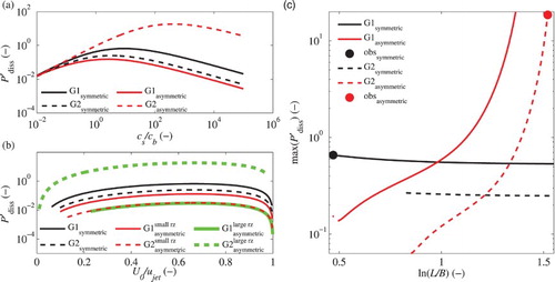
Table 1. Reservoir geometries used for Figs and
To identify the switch between symmetric and asymmetric flow patterns, we performed the same analysis for both geometries but with different reservoir lengths. Plotting the maximum of energy dissipation for each single geometry against shows that for relatively short reservoirs the symmetric flow pattern dissipates more energy within the shear layer between jet and recirculation zone, while for relatively long reservoirs, the asymmetric flow pattern dissipates more energy (Fig. c). Depending on the ratio B/b the point where the prevailing flow pattern switches varies, which is (qualitatively) in accordance with observations (Fig. ).
To quantitatively compare the switch between the two flow patterns we performed the same analysis for a range of L/B and B/b values. Comparing this with the empirical switch between symmetric and asymmetric flow reveals reasonable results depending on the values of the three free parameters (Fig. ). Best correspondence is obtained when the reattachment length of the empirical relation is used in combination with a centre point of the small recirculation zone at
and
. Longer reattachment lengths move the theoretical switch to the right, while changes in the centre point of the small recirculation zone slightly affects the slope of the line, while also moving it in a horizontal direction. Interestingly, an empirical reattachment length – which is independent on the reservoir length – results in straighter lines than if it is dependent on the reservoir length. From the two different empirical relations,
most closely follows the slope of the empirical switch.
Figure 6. Comparison of maximum energy dissipation related switch and empirical switch between symmetric and asymmetric flow patterns. The different colours represent different values of the free parameters (i.e. the reattachment length and the relative position (
and
) of the centre point of the small recirculation zone)
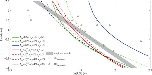
Figure 7. 2D simulated flow fields of a (a) symmetric flow pattern (test 5 of Camnasio et al., Citation2014, and Geometry 1 in Table ) and (b) asymmetric flow pattern (test 7 of Camnasio et al., Citation2014, and Geometry 2 in Table ). The lines correspond to the triangular flow patterns used in this study: In (b) the reattachment length is used, since this geometry is far enough from the switch to a symmetric flow pattern (see red circle in Fig. c)
In this study, we hypothesized that the reattachment length could also be derived by maximizing energy dissipation. However, this is not the case: in our model set-up, the smaller the reattachment length, the higher the dissipated energy. Thus maximum energy dissipation is achieved when the contact area between the jet and the large recirculation zone is maximum. However, simulations with such short reattachment lengths do not lead to switches between symmetric and asymmetric flow patterns which are close to the empirical ones.
4. Discussion
In our simplified model, three parameters were left unconstrained (,
and
). Although this allowed a sensitivity analysis on these three parameters, we could not define them a priori. Our hypothesis that the best reattachment length would follow from the value leading to maximum energy dissipation has to be rejected. This is because energy dissipation increased with increasing reattachment length, and, therefore, no maximum in dissipation exists along this degree of freedom. Although we were not able to predict the reattachment length, it is important to note that the empirical reattachment length gave best results when predicting the switch between symmetric to asymmetric flow patterns, with
revealing a better fit than
, supporting our hypothesis that energy dissipation is indeed maximized.
The two other free parameters defined the centre point of the small recirculation zone. It was found that the values of and
outperformed the model set-up using the centroid (
) as the centre point. When compared against the 2D flow fields simulated by Camnasio et al. (Citation2014) – which correspond closely to observations – we see that in their simulations the centre point is also at
and
(Fig. b); albeit that in their 2D simulations, the small recirculation zone is not exactly triangular, but curved. This implies that the real centre point is not as close to the side of the recirculation zone as in our triangular set-up. Furthermore, the centre points of the symmetric flow pattern (Fig. a) and of the large recirculation zone of the asymmetric flow pattern (Fig. b) were constrained at locations very close to their simulated centre points.
It is also worth noting that due to our assumption of a constant jet width in combination with the constraint to fix the point of the large recirculation zone (which always lies on a 1:1 line passing the upper right corner of the reservoir), the large recirculation zone cannot be constructed for very short or very long reservoir lengths. In these cases, the centre point of the large recirculation zone lies outside the recirculation zone, which is physically not possible. We therefore excluded results where the centre point lies outside the recirculation zone. All lines presented in Fig. are in the range where the centre point lies within the recirculation zone.
Besides these free parameters, the largest simplifications in our model are of course the schematization of the flow fields and the lumped treatment of the energy balance. Of the former, not only the shape of the jet, but especially the mathematical description of the recirculation zones, vary from the observations. As explained in Section 2.1, we introduced the linear flow distribution in the local η-direction of each triangle to accommodate a velocity ratio for an infinite large friction coefficient
. However, this is not the flow pattern observed in reality. In reality, the flow pattern is more circular as sketched in Fig. . A possible workaround to obtain such a flow pattern for relatively small values of
, while reaching a velocity ratio of unity at infinite large
would be to describe the flow field along the sides of the recirculation zone as a power function:
, in which the power n depends on the friction coefficient
: e.g.
. Assuming a linear decrease in u with y and having a similar formulation for the vertical velocity v, the flow field for a rectangular recirculation zone, as in the symmetric flow pattern, can be written as:
(8)
(9)
which can be filled into Eq. (Equation2
(1b) ) and subsequently be solved for
.
However, this mathematical description only applies to the symmetric cases. We were not able to find a comparable formulation for the more complex trapezoidal recirculation zone in the asymmetric case. Therefore, if, and how, this can be improved remains an open question.
The lumped treatment of the energy balance (Eq. (Equation1(1a) )), is another simplification in which local friction terms are lumped into one effective variable and in which there is a strict separation between the jet and the recirculation zone. In reality, there is a smooth transition in flow velocity between the two (see e.g. Fig. 5 of Camnasio et al., Citation2014), which makes it not possible to directly compare the velocity ratios
of our optimization with observed ones.
What remains is the question of why this system would organize in order to maximize energy dissipation within the shear layer. At this moment we have no definite explanation. However, it is clear that when the friction coefficient is very small () no energy is transferred from the jet to the recirculation zone. In other words, friction in the shear layer is needed to set the recirculation zone in motion. Furthermore, with increased friction, frictional losses (and thus energy dissipation) occurs.
However, this only explains why energy dissipation increases with increasing energy transfer from the jet to the recirculation zone. It does not explain why energy dissipation decreases again after its maximum is reached. An explanation could be that at extreme high friction () the velocity difference in the shear layer becomes zero, meaning that also here no energy is transferred from the jet to the recirculation zone. If no energy is transferred, the velocity in the recirculation zone would decrease, leading to a velocity difference in the shear layer, and thus to frictional losses. Thus, at the two extremes, there would be no energy transfer, while at intermediate values there is. Along this line of reasoning, frictional loss in the shear layer is a surrogate for energy transfer from the jet to the recirculation zones, and maximum energy dissipation is equivalent to maximum power and maximum entropy production (Kleidon, Citation2016): principles which have been demonstrated to have predictive power.
5. Conclusions
In this study we aimed to explain observed flow patterns in rectangular shallow reservoirs, and especially the switch between symmetric and asymmetric recirculation zones on both sides of the main jet. We demonstrated that, for a certain flow field, the momentum transfer from the jet to the recirculation zone is optimized in order to have maximum energy dissipation in the shear layer between the jet and recirculation zone. If this optimized energy dissipation is higher for a symmetric flow field than for an asymmetric flow field, the occurring flow field will be symmetric; if it is the other way around, it will be asymmetric.
A limited number of parameters are not constrained in our simplified model, namely the reattachment length and the centre of the small recirculation zone in the asymmetric case. We showed that, depending on the value of these free parameters, our hypothesis closely reproduces the observed switch between symmetric and asymmetric flow patterns. Best correspondence occurred when the free parameters were given the observed values, which suggests that our hypothesis is correct. We consider it very likely that the discrepancy between our modelled switch and the observed one is caused by the simplifications and assumptions necessary in our mathematical description of the flow fields. Due to these simplifications it was also not possible to directly compare our optimized velocity ratios with observed ones.
Therefore, “proof” that the system maximizes energy dissipation in the shear layer is reliant on the switch between the two flow patterns when observed geometric features, such as reattachment length or centre points of recirculation zones, are used in our model description.
Assuming that our used principle is correct, these flow patterns organize such that energy dissipation is maximized. This internal optimization causes macroscale structures, which we observe as recirculation zones. This makes it possible to perform projections of these macroscale features of flow patterns without knowing small scale flow processes. From an engineering perspective, this theory could prove very valuable, particularly at the early stage of reservoir design.
Of course, care should be taken with the flow ranges for which a certain macroscale description is valid. For this reason, our model description is only valid for describing symmetric and the first asymmetric flow pattern. At this stage it cannot be used for longer reservoirs in which the jet jumps over to the other side of the reservoir (Dufresne et al., Citation2010b), or even starts meandering (Peltier et al., Citation2014). This is subject to further investigations.
Notation
| b | = | width of inlet and outlet channels (L) |
| B | = | lateral expansion of reservoir (L) |
| cb | = | friction coefficient between recirculation zone and bottom (–) |
| cs | = | fluid-fluid friction coefficient (–) |
| cx | = | x-coordinate of the centre point of the small recirculation zone (L) |
| cy | = | y-coordinate of the centre point of the small recirculation zone (L) |
| F | = | Froude number (–) |
| g | = | acceleration of gravity (L T−2) |
| h | = | water height (L) |
| l | = | distance along the contact area between jet and recirculation zone (L T−1) |
| L | = | reservoir length (L) |
| Lbi | = | length of the base of triangle i (L) |
| LHi | = | height of triangle i (L) |
| Lre | = | reattachment length (L) |
| Ls | = | total length of the contact area between jet and recirculation zone (L T−1) |
| n | = | power in Eq. (8 and 9) |
| Pjet | = | rate of work performed by the jet on the recirculation zone (M L2T−3) |
| Prz | = | rate of work received by the recirculation zone from the jet (M L2T−3) |
| Pbot | = | dissipation of rate of work by bottom friction in the recirculation zone (M L2T−3) |
| Pdiss | = | energy dissipation within the shear layer between jet and recirculation zone (M L2T−3) |
| Q | = | discharge (L T−3) |
| S | = | surface area of recirculation zone (L2) |
| u | = | water velocity (L T−1) |
| ujet | = | velocity of jet (L T−1) |
| urc | = | velocity component of recirculation zone in the x dimension (L T−1) |
| Ui | = | maximum velocity in triangle i (L T−1) |
| vrc | = | velocity component of recirculation zone in the y dimension (L T−1) |
| x | = | length in global coordinate system (L) |
| y | = | width in global coordinate system (L) |
| η | = | locale coordinate following the base of the triangle (L) |
| ξ | = | locale coordinate perpendicular to the base of the triangle (L) |
| ρ | = | water density (M L−3) |
Acknowledgements
We would like to thank the associate editor and three anonymous reviewers for their supportive comments, which helped us to improve the manuscript.
ORCID
Martijn C. Westhoff http://orcid.org/0000-0002-8413-5572
Benjamin Dewals http://orcid.org/0000-0003-0960-1892
Additional information
Funding
References
- Camnasio, E., Erpicum, S., Archambeau, P., Pirotton, M., & Dewals, B. (2014). Prediction of mean and turbulent kinetic energy in rectangular shallow reservoirs. Engineering Applications of Computational Fluid Mechanics, 8(4), 586–597. doi: 10.1080/19942060.2014.11083309
- Camnasio, E., Erpicum, S., Orsi, E., Pirotton, M., Schleiss, A. J., & Dewals, B. (2013). Coupling between flow and sediment deposition in rectangular shallow reservoirs. Journal of Hydraulic Research, 51(5), 535–547. doi: 10.1080/00221686.2013.805311
- Camnasio, E., Orsi, E., & Schleiss, A. J. (2011). Experimental study of velocity fields in rectangular shallow reservoirs. Journal of Hydraulic Research, 49(3), 352–358. doi: 10.1080/00221686.2011.574387
- Carnot, S. (1824). Réflexions sur la puissance motrice du feu et sur les machines propres a développer cette puissance. Paris: Bachelier.
- Choufi, L., Kettab, A., & Schleiss, A. J. (2014). Bed roughness effect on flow field in rectangular shallow reservoir [effet de la rugosité du fond d'un réservoir rectangulaire à faible profondeur sur le champ d'écoulement]. La Houille Blanche, 5, 83–92. doi: 10.1051/lhb/2014054
- Dewals, B., Erpicum, S., Archambeau, P., & Pirotton, M. (2012). Experimental study of velocity fields in rectangular shallow reservoirs. Journal of Hydraulic Research, 50(4), 435–436. doi: 10.1080/00221686.2012.702856
- Dewals, B. J., Kantoush, S. A., Erpicum, S., Pirotton, M., & Schleiss, A. J. (2008). Experimental and numerical analysis of flow instabilities in rectangular shallow basins. Environmental Fluid Mechanics, 8(1), 31–54. doi: 10.1007/s10652-008-9053-z
- Dominic, J. A., Aris, A. Z., Sulaiman, W. N. A., & Tahir, W. Z. W. M. (2016). Discriminant analysis for the prediction of sand mass distribution in an urban stormwater holding pond using simulated depth average flow velocity data. Environmental Monitoring and Assessment, 188(3), 1–15. doi: 10.1007/s10661-016-5192-8
- Dufresne, M., Dewals, B. J., Erpicum, S., Archambeau, P., & Pirotton, M. (2010a). Classification of flow patterns in rectangular shallow reservoirs. Journal of Hydraulic Research, 48(2), 197–204. doi: 10.1080/00221681003704236
- Dufresne, M., Dewals, B. J., Erpicum, S., Archambeau, P., & Pirotton, M. (2010b). Experimental investigation of flow pattern and sediment deposition in rectangular shallow reservoirs. International Journal of Sediment Research, 25(3), 258–270. doi: 10.1016/S1001-6279(10)60043-1
- Dufresne, M., Dewals, B. J., Erpicum, S., Archambeau, P., & Pirotton, M. (2011). Numerical investigation of flow patterns in rectangular shallow reservoirs. Engineering Applications of Computational Fluid Mechanics, 5(2), 247–258. doi: 10.1080/19942060.2011.11015368
- Hergarten, S., Winkler, G., & Birk, S. (2014). Transferring the concept of minimum energy dissipation from river networks to subsurface flow patterns. Hydrology and Earth System Sciences, 18(10), 4277–4288. doi: 10.5194/hess-18-4277-2014
- Howard, A. D. (1990). Theoretical model of optimal drainage networks. Water Resources Research, 26(9), 2107–2117. doi: 10.1029/WR026i009p02107
- Kantoush, S. A. (2008). Experimental study on the influence of the geometry of shallow reservoirs on flow patterns and sedimentation by suspended sediments (PhD thesis 4048). EPFL Lausanne, Switzerland.
- Kantoush, S. A., Bollaert, E., & Schleiss, A. J. (2008). Experimental and numerical modelling of sedimentation in a rectangular shallow basin. International Journal of Sediment Research, 23(3), 212–232. doi: 10.1016/S1001-6279(08)60020-7
- Kleidon, A. (2016). Thermodynamic foundations of the earth system. Cambridge: Cambridge University Press.
- Kleidon, A., & Renner, M. (2013). Thermodynamic limits of hydrologic cycling within the earth system: Concepts, estimates and implications. Hydrology and Earth System Sciences, 17(7), 2873–2892. doi: 10.5194/hess-17-2873-2013
- Kleidon, A., Zehe, E., Ehret, U., & Scherer, U. (2013). Thermodynamics, maximum power, and the dynamics of preferential river flow structures at the continental scale. Hydrology and Earth System Sciences, 17(1), 225–251. doi: 10.5194/hess-17-225-2013
- Langbein, W., & Leopold, L. (1966). River meanders – theory of minimum variance (Tech. Rep. No. 422-H). Washington, DC: USGS.
- Lorenz, R. D., Lunine, J. I., Withers, P. G., & McKay, C. P. (2001). Titan, Mars and Earth: Entropy production by latitudinal heat transport. Geophysical Research Letters, 28, 415–418. doi: 10.1029/2000GL012336
- Michalec, B. (2014). The use of modified annandale's method in the estimation of the sediment distribution in small reservoirs: A case study. Water (Switzerland), 6(10), 2993–3011.
- Paltridge, G. W. (1979). Climate and thermodynamic systems of maximum dissipation. Nature, 279, 630–631. doi: 10.1038/279630a0
- Peltier, Y., Erpicum, S., Archambeau, P., Pirotton, M., & Dewals, B. (2014). Experimental investigation of meandering jets in shallow reservoirs. Environmental Fluid Mechanics, 14(3), 699–710. doi: 10.1007/s10652-014-9339-2
- Peng, Y., Zhou, J. G., & Burrows, R. (2011). Modeling free-surface flow in rectangular shallow basins by using lattice boltzmann method. Journal of Hydraulic Engineering, 137(12), 1680–1685. doi: 10.1061/(ASCE)HY.1943-7900.0000470
- Potter, M. C., Wiggert, D. C., Hondzo, M., Shih, T. I. P., & Chaudhry, K. K. (2010). Mechanics of fluids (3rd ed.). Stamford, CT: Cengage Learning.
- Rinaldo, A., Rodríguez-Iturbe, I., Rigon, R., Bras, R. L., Ijjasz-Vasquez, E., & Marani, A. (1992). Minimum energy and fractal structures of drainage networks. Water Resources Research, 28(9), 2183–2195. doi: 10.1029/92WR00801
- Rodriguez-Iturbe, I., Rinaldo, A., Rigon, R., Bras, R. L., Ijjasz-Vasquez, E., & Marani, A. (1992). Fractal structures as least energy patterns: The case of river networks. Geophysical Research Letters, 19(9), 889–892. doi: 10.1029/92GL00938
- Rodríguez-Iturbe, I., Rinaldo, A., Rigon, R., Bras, R. L., Marani, A., & Ijjász-Väsquez, E. (1992). Energy dissipation, runoff production, and the three-dimensional structure of river basins. Water Resources Research, 28(4), 1095–1103. doi: 10.1029/91WR03034
- Secher, M., Hervouet, J. M., Tassi, P., Valette, E., & Villaret, C. (2014). Numerical modelling of two-dimensional flow patterns in shallow rectangular basins. In P. Gourbesville, J. Cunge, & G. Caignaert (Eds.), Advances in hydroinformatics: Simhydro 2012 – new frontiers of simulation (pp. 499–510). Singapore: Springer Singapore.
- Tarpagkou, R., & Pantokratoras, A. (2013). Cfd methodology for sedimentation tanks: The effect of secondary phase on fluid phase using dpm coupled calculations. Applied Mathematical Modelling, 37(5), 3478–3494. doi: 10.1016/j.apm.2012.08.011
- Tsavdaris, A., Mitchell, S., & Williams, J. B. (2015). Computational fluid dynamics modelling of different detention pond configurations in the interest of sustainable flow regimes and gravity sedimentation potential. Water and Environment Journal, 29(1), 129–139. doi: 10.1111/wej.12086
- Zehe, E., Ehret, U., Blume, T., Kleidon, A., Scherer, U., & Westhoff, M. (2013). A thermodynamic approach to link self-organization, preferential flow and rainfall–runoff behaviour. Hydrology and Earth System Sciences, 17(11), 4297–4322. doi: 10.5194/hess-17-4297-2013
- Zhou, J. G., Liu, H., Shafiai, S., Peng, Y., & Burrows, R. (2010). Lattice boltzmann method for open-channel flows. Proceedings of the Institution of Civil Engineers: Engineering and Computational Mechanics, 163(4), 243–249.