SPHysics simulation of laboratory shallow free surface turbulent flows over a rough bed

ABSTRACT

In this paper, the smoothed particle hydrodynamics method is used to simulate experimental shallow free surface turbulent flows over a rough bed made of regularly packed uniform spheres. The numerical program is based on the open source code SPHysics and significant improvement is made in the turbulence modelling and rough bed treatment within the code. A modified sub-particle-scale eddy viscosity model is proposed to simulate the effect of turbulence transfer mechanisms in the highly-sheared free surface flow, and a drag force term is introduced into the momentum equation as a source term to account for the existence of the bed roughness. To validate the numerical model, a laboratory experiment is carried out to study shallow, turbulent flow behaviour under different flow conditions. The SPH simulations are then compared with the flow velocity, shear stress and turbulent intensity profiles measured via acoustic doppler velocimeters. Several issues with regard to the rough bed hydraulics are investigated, including the study of water surface behaviour and its interaction with the bulk flow.

Keywords:

• Drag force
• rough bed
• shallow free surface flow
• SPHysics
• SPS eddy viscosity model
• water surface behaviour

1 Introduction

Free surface flows in rivers and man-made channels are of significant importance in the field of hydrodynamics and hydraulic engineering. These types of flow are often found over rough surfaces sometimes with complex topographies and characterized by spatial and temporal deformations of the free surface. When the flow depth is shallow, the influence of the bed roughness can significantly modify the structure of the flow. The hydraulics of shallow rough bed open channel flows has both theoretical and engineering value in view of the need to quantify bed resistance, which can provide important information for those concerned with flood control and environment protection. However, there have been limited studies on the water surface behaviour of shallow free surface flows and its relationship with the underlying turbulent flow structures due to the difficulty in obtaining laboratory measurements and the spatial resolution constraint in numerical simulations.

In the past few decades, numerical simulations on the basis of mesh-based approaches have been widely used for various free surface flows. The two most popular mesh-based approaches for simulating free surface flows are the mark-and-cell (MAC) and volume-of-fluid (VOF) techniques. In these methods, the free surface flow properties are computed through the Navier–Stokes (N-S) equations over a stationary mesh, which can give rise to numerical diffusion due to the advection term in the N-S equations. This makes the application of the mesh-based approach challenging for free surface flows in which the water surface is specified as an arbitrarily moving boundary. In recent years, the mesh-free smoothed particle hydrodynamics (SPH) technique, which was first introduced by Gingold and Monaghan (1977) to solve astrophysical problems, has been developed and successfully used for the simulation of a wide range of computational fluid dynamics (CFD) applications. These include wave breaking and overtopping (Monaghan & Kos, 1999), multi-phase flow with a sharp material interface (Colagrossi & Landrini, 2003; Hu & Adams, 2007), and dam-break flow (Gómez-Gesteira & Dalrymple, 2004). More advanced turbulent closure modelling techniques in SPH have been reviewed by Violeau and Issa (2007) and used by Dalrymple and Rogers (2006) for wave impact on a coastal defence. These techniques are based on the pioneering work of Gotoh, Shibahara, and Sakai (2001), who proposed the most commonly used turbulent modelling technique in mesh-free particle method: the sub-particle scale (SPS) model. Due to its capability and flexibility in simulating complex flow situations, SPH has become a competitive alternative to mesh-based methods. Unlike mesh-based approaches, SPH is a purely Lagrangian meshless technique in which the fluid domain is discretized into a set of particles carrying various physical properties, and these particles are moved according to the kernel influence of their neighbouring particles. Consequently, all the terms in the governing equations are expressed as the interaction between each reference particle and its neighbours, so no computational grid is needed in the solution domain.

Although SPH has been successfully used for the simulation of different fluid phenomena, such as in coastal hydrodynamics, only a small number of researchers have applied this technique to open channel free surface flows. In the literature, Federico, Marrone, Colagrossi, Aristodemo, and Antuono (2012) and Shakibaeinia and Jin (2010) used SPH to study a uniform laminar open channel flow of low Reynolds Number and validated their model by initializing and updating the analytical velocity and pressure profiles on the inflow boundary. Later Meister, Burger, and Rauch (2014) used the same numerical technique for steady laminar open channel flows with different water viscosities. Their results demonstrated that for highly viscous flow, the streamwise velocities agreed well with analytical solutions; however, when the viscosity was reduced close to the actual value of water, the predicted velocities gradually deviated from the analytical predictions. Džebo, Žagar, Krzyk, Četina, and Petkovšek (2014) performed SPH modelling of dam-break flow through a narrow rough valley, in which two different methods of defining the terrain roughness were used for the hydraulically smooth and rough terrains, respectively. SPH techniques have also been used to simulate hydraulic jumps, as documented by López, Marivela, and Garrote (2010), Chern and Syamsuri (2013) and De Padova, Mossa, Sibilla, and Torti (2013), and various turbulent closure models were included in these studies. However, there were no detailed quantification of the velocity and shear stress profiles for the shallow free surface turbulent flows over a hydraulically rough bed, and there was also a lack of information on the water surface fluctuations and their relationships with the underlying turbulent flow structure. More robust treatment of the flow turbulence and rough bed boundary would enable SPH models to be applied to more practical engineering situations.

In this paper, we aim to use the weakly compressible SPH (WCSPH) open source code, SPHysics (http://www.sphysics.org), to investigate shallow free surface turbulent flows over a rough bed and then validate the numerical results using our laboratory measurements. To improve the model capacity to address the effects of turbulence, an improved SPS eddy viscosity model is proposed, in which the fixed Smagorinsky constant is replaced by a mixing length formulation. In addition, to account for the effect of bed roughness, a drag force term is added to the momentum equation as a source term to compute the resistance shear stress. We use this numerical model to predict the time-averaged streamwise flow velocity and shear stress, and turbulent intensity profiles, and also examine the dynamic behaviour of water surface fluctuations along the streamwise direction. These are compared with our experimental measurements.

Here it should be mentioned that one of the major objectives in this paper is to use the mesh-free SPH modelling approach to investigate the water surface fluctuations. This is not commonly studied and is difficult to address by using the standard grid-based numerical models. In the literature, it has been found that the free surface of turbulent shallow open channel flow is never completely flat, since it is disturbed by the underlying turbulent flow structures and advecting capillary-gravity waves. Some preliminary experimental studies have been conducted to establish the links between water surface features and subsurface turbulent flow structures. For example, Kumar, Gupta, and Banerjee (1998) found a persistent structure on the water–air interface that can be classified into different types according to the pattern of the turbulent burst features. Smolentsev and Miraghaie (2005) observed that three types of the disturbance always co-exist on the free surface: capillary waves, gravity waves and turbulent waves. The latter was generated due to the interactions between the bulk flow and water surface, and was found to be the most dominant component. In a more recent study, Horoshenkov, Nichols, Tait, and Maximov (2013) experimentally studied the free surface and its interactions with the underlying turbulence of shallow free surface flows over a gravel bed. They demonstrated that the free surface fluctuations are strongly correlated with the bulk flow properties. This would constitute an interesting field to apply the SPH simulation technique, in order to fully explore its potential as an emerging engineering tool in free surface turbulent flows.

2 SPH numerical model

2.1 Governing equations and SPH formulations

In the SPH numerical scheme the following mass and momentum conservation equations of a compressible Newtonian fluid are solved: (1) (2) where is particle velocity vector, is density, is pressure, is gravitational acceleration, is kinematic viscosity, is turbulent shear stress, and is time. The notation is used to denote the Lagrangian derivative. Hence the fluid particle movement is computed by the following equation, where is the particle position vector: (3) In the SPH framework, a reference particle interacts with the neighbouring particle within a kernel influence domain following a weighting function , where is the distance between particles and , and is the kernel smoothing length. In SPH approximations, the value of any vector quantity or physical scalar of a reference particle , and its gradient , can be estimated by the following discretized summation equations carried out for all particles located inside the kernel influence domain as: (4a) (4b) where is the mass of neighbouring particle , is the density of neighbouring particle, is the value of the quantity at point , is the value of the quantity at point , is the gradient of the quantity at the point , and is the gradient of the kernel function at particle . Considering computational efficiency and accuracy, the kernel function is based on the cubic spline.

By applying the SPH discretization to mass conservation Eq. (1), the changing rate of density of particle with respect to its neighbouring particles can be computed as: (5) where is defined. Similarly, all terms in the momentum Eq. (2) can be transformed into the SPH forms. The following anti-symmetric form of the pressure gradient is one commonly used: (6) Khayyer and Gotoh (2010) simplified the laminar stress term in the following SPH formulation: (7) To close the system of governing equations for a slightly compressible fluid flow, the following equation of state is employed to determine the fluid pressure (Monaghan & Kos, 1999): (8) where , is the speed of sound at a reference density, is 1000 kg m⁻³ and the reference density is usually taken as the density of fluid at the free surface, and  = 7 is the polytrophic constant. Using a value corresponding to the real speed of sound in water can lead to a very small time step to achieve the numerical stability required by the Courant–Fredrich–Levy condition. Monaghan and Kos (1999) suggested that the minimum speed of sound be about 10 times greater than the maximum bulk flow velocity. This keeps the density variations to less than 1%. For the considered free surface shallow steady flows the density fluctuations (with respect to the reference value) are expected to be rather small. Therefore, the above Eq. (8) could also be conveniently linearized without the loss of accuracy.

In a real SPH computation, with regard to Eq. (3), the fluid particles are actually moved by using the XSPH variant as proposed by Monaghan and Kos (1999), as follows: (9) where is constant (0–1), and is averaged density. The idea behind the XSPH variant is that a fluid particle moves with a velocity that is close to the averaged velocity of its neighbouring particles depending on the coefficient . The main rationale of using this approach in coastal hydrodynamics is to prevent the fluid particles from penetrating each other, and thus to ensure the simulations are stable. In our free surface open channel flow simulations, we found that a non-zero value of significantly dampens the physical velocity fluctuations and the velocity gradient was reduced along the flow depth. Therefore, the XSPH variant was not used by assigning a zero value to in Eq. (9).

2.2 SPHysics code

SPHysics code (http://www.sphysics.org) is a free open-source SPH code that was released in 2007 and developed jointly by the researchers at Johns Hopkins University (Baltimore, MD, USA), University of Vigo (Vigo, Spain), University of Manchester (Manchester, UK) and University of Roma La Sapienza (Rome, Italy). It is programmed in the FORTRAN language, and developed specifically for the free-surface hydrodynamics (Gomez-Gesteira et al., 2012). In this paper, we use the SPHysics to carry out the simulations of shallow turbulent free surface flow over a rough bed surface, after modifying the code by adding a turbulent closure technique and a rough bed treatment.

In SPHysics, four different time integration schemes are implemented. The predictor–corrector solution is used in our studies due to being explicit in the time integration and straightforward to implement. It is second-order accurate in the time domain. To reduce the particle noise in the pressure field, a density filtering operation is carried out every 20 to 30 time steps to smooth out the density and pressure noise. Two density filters are available in the SPHysics code, the Shepard filter and the moving least squares (MLS) filter.

2.3 Boundary conditions

In SPH solid wall boundaries are treated mainly to ensure that the fluid particles cannot penetrate the wall, and that the non-slip boundary conditions are satisfied. Different wall treatments have been used in SPHysics, and the dynamic particle approach (Dalrymple & Knio, 2001) is adopted in the present study, because all of the wall particles can be computed inside the same loop as the inner fluid particles.

The treatment of inflow and outflow boundaries in SPH is important for the simulation of open channel flows. In recent years, different inflow and outflow techniques have been implemented. For example, Lee et al. (2008) used a periodic open boundary by which the fluid particles that leave the computational domain through the outflow boundary are instantly re-inserted on the inflow boundary, and the fluid particles close to one open lateral boundary should interact with the particles near the complementary open lateral boundary on the other side of the computational domain. The periodic boundary treatment is simple and straightforward to implement and it demonstrates good performance on the boundaries of symmetric geometry. Since the open channel flow in our study is considered as uniform and steady flow, and the main objective is to investigate the turbulence model and treatment of the rough bed boundary, we simply use the periodic open boundary provided by SPHysics (Gomez-Gesteira et al., 2012) without further investigation.

2.4 Improved SPS turbulence model with non-constant Smagorinsky coefficient

Since our model is applied to fully-turbulent open channel flows, an appropriate turbulence model is required to close the system of the momentum equation. In SPHysics, the turbulent shear stress is modelled by using an eddy viscosity based SPS model initially described by Gotoh et al. (2001) in the momentum Eq. (2). The SPS turbulent stress is based on the eddy viscosity assumption as follows: (10) where is SPS shear stress component, is turbulent eddy viscosity (where is Smagorinsky constant, , is local strain rate, is SPS strain component), is turbulent kinetic energy, is Kronecker’s delta,  = 0.0066, and is initial particle spacing. In many SPH applications in coastal hydrodynamics, C_s is regarded as a constant, 0.1–0.2.

Although this benchmark formulation has been successfully used in a number of coastal applications, very limited studies have been reported on the effectiveness of such a turbulence closure in open channel flow. In our model test of laboratory turbulent rough bed open channel flow, it was found that the value of has a significant influence on the streamwise flow velocity profiles as shown in Fig. 1 (for flow condition (7) as shown in Table 1). It is apparent that increasing resulted in a decrease in both the streamwise velocity and its gradient due to enhanced numerical dissipation. To study this phenomenon, different values of C_s were provided for each flow condition in Table 1 (designed to match our laboratory experiment as detailed later) based on the best match between the measured and computed time-averaged velocity profiles.

Figure 1 Influence of value on time-averaged streamwise velocity profile for flow condition (7) (dashed lines correspond to roughness top and bottom)

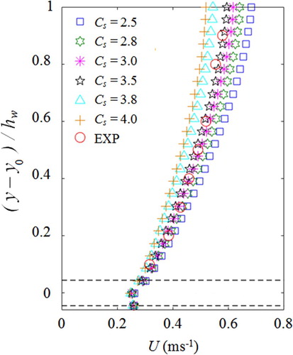
Table 1 Summary of experimental flow conditions

Flow condition	Uniform depth hw (mm)	Mean velocity (m s^−1)	Shear velocity u* (m s^−1)	Bed slope (–)	Reynolds Number (–)	Froude Number (–)	Hydraulic roughness ks (mm)	Smagorinsky constant (–)
1	40	0.28	0.039	0.004	11200	0.447	35	1.88
2	50	0.35	0.044	0.004	17000	0.499	35	2.17
3	60	0.26	0.034	0.002	13200	0.339	30	0.60
4	70	0.33	0.037	0.002	23100	0.398	28	1.04
5	70	0.36	0.045	0.003	30800	0.434	30	2.54
6	80	0.42	0.048	0.003	33600	0.474	28	3.20
7	90	0.47	0.051	0.003	42300	0.500	28	3.50
8	100	0.43	0.044	0.002	43000	0.434	22	2.20

An analysis has also been made of the relationships between and the flow depth h_w, channel bed slope , flow Reynolds Number and shear velocity , and the results are presented in Fig. 2. As shown in Table 1, the shear velocity is calculated as , where  = 9.81 m s⁻². The Reynolds Number is calculated from and Froude Number , where is depth-averaged mean flow velocity. The hydraulic roughness k_s is obtained by fitting the streamwise velocity profile measured in the centre of flume to the log-law of rough bed turbulent flow as given by: (11) where , is von Kármán constant (0.41), (where y is vertical distance from the bed boundary), (where k_s is hydraulic roughness), and is constant (8.5 for the rough walls).

Figure 2 Relations between and (a) flow depth and channel slope ; (b) Reynolds Number ; and (c) shear velocity u*

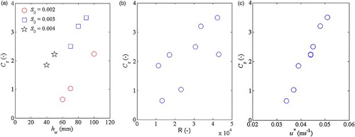
Figure 2 shows that has a positive correlation with the flow depth and channel bed slope but seems to be independent of the Reynolds Number . A strong positive correlation has also been found between and the shear velocity u*, which indicates that could carry information on the near-bed streamwise velocity gradient. The C_s values in present study were found to be 0.6–3.5 as listed in Table 1 for the shallow turbulent flows over a rough bed. This is significantly larger than the common C_s values used in other SPH applications, for example, in coastal hydrodynamics a value of 0.1–0.2 is often recommended. This difference can be attributed to the fact that the relevant processes in both applications are different, and since in open channel flows the bed roughness is one of the dominant physical factors, a more refined treatment of the bed resistance process in the overall momentum balance is therefore important.

However, the obtained values of in Table 1 have been found to provide turbulent shear stresses much smaller than the measured ones. We therefore decided to use the classic mixing length theory to modify the SPS model of Gotoh et al. (2001), by replacing the product of with a mixing length formulation, which should be more realistic for open channel flows as it allows the use of a function that depends on the distance from the bed boundary. In a two-dimensional form, the relevant equation is represented as: (12) where l_m is mixing length, which describes the typical turbulent eddy size. Among many expressions to determine l_m, a common one first proposed by Nezu and Nakagawa (1993), and further applied in the open channel flows by Stansby (2003), has the following form: (13) where is vertical distance measured from the zero-velocity level, H is total water depth, and is a constant (typically being 0.09).

By adopting the above mixing length approach, we would expect a better representation of the impact of the rough bed on open channel flows, since the model coefficients now depend on the local flow conditions and the size of the internal flow structures, thought to depend on the distance from the rough bed, to internally transfer the momentum within the fluid.

2.5 Treatment of rough bed using drag force term in momentum equation

As mentioned before, currently the fixed channel bed is simulated by using the dynamic SPH particle approach (Dalrymple & Knio, 2001). However, this boundary treatment behaves like a hydraulic smooth bed and cannot adequately reflect the frictional force generated by the roughness elements such as the spherical particles. To enable the model to simulate our experiment of a hydraulically rough bed, the drag force due to the existence of the roughness element on the channel bottom must be addressed. This can be quantified by the following: (14) where is fluid drag force, is reference area of the bed obstacle, is dimensionless drag coefficient, and is reference velocity. The vertical lift force was neglected in the current 2D simulations due to the magnitude of the vertical velocities being only a few per cent of the streamwise velocities and so was believed to have no significant influence on the flow. Although the non-slip boundary conditions cannot be accurately enforced due to the use of the dynamic particle approach (Dalrymple & Knio, 2001), our treatment of the rough bed by adding a drag force term should help to better fulfil this requirement.

The original idea of incorporating a drag force term into the momentum equation to treat the bed roughness was proposed by Gotoh and Sakai (1999) for a plunging wave interaction with the porous bed. This was later used by Khayyer and Gotoh (2010) for the dam-break flows over a frictional bed. The determination of the drag coefficient is a key factor in the simulations of flow over bed obstacles. In the literature the drag coefficient has been found to be dependent on the shape of the bed obstacles and the local flow Reynolds Number. Although different values of have been experimentally found for spherical bed particles, we use the coefficient as measured by Schmeeckle, Nelson, and Shreve (2007). They found that the averaged values of drag coefficient were around 0.76 for turbulent flows with a Reynolds Number range of 50,000–200,000 and mean velocity of 0.2–0.9 m s⁻¹. In our simulations, a value of  = 0.76 was initially used for the flow conditions (1) and (2) in Table 1, and the computed time-averaged velocity profiles were found to be slightly faster than the measured ones. We then decided to slightly increase this coefficient to  = 0.8, and this provided a better match with measured data. This slightly increased value was fixed for all the flow conditions.

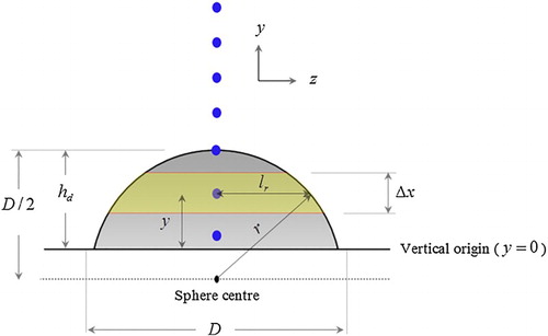
The reference area in Eq. (14) is usually taken as the obstacle frontal area perpendicular to the flow direction, whereas the reference velocity is related to the averaged streamwise flow velocity acting on the area. In our drag force model, the drag area of the bed roughness element is visualized in Fig. 3. It shows that the area is not constant for a spherical shape, and decreases toward the top of the sphere, resulting in a decrease in the drag force . Thus Eq. (14) becomes a function of the vertical distance by following Fig. 3, in which the yellow highlighted drag area for each fluid particle within the roughness height is mathematically determined by , where is the length of half chord calculated by . By substituting and into Eq. (14), the drag force imposed on a fluid particle located at level y can be computed as: (15) It is necessary to compute the drag force per unit volume of the fluid in order to be dimensionally consistent with the momentum Eq. (2). The volume over which the drag force acts is equal to so in the SPH form Eq. (15) becomes: (16) The position of vertical origin ( = 0) for the velocity profile, at which  ≈ 0.0 m s⁻¹, can be set at a distance of below the top of the roughness element. The value of (roughness height) should be determined in such a way that the streamwise velocity distribution can fit the log-law given by Eq. (11). In the experimental study using hemispherical roughness elements of diameter , slightly different values of have been documented. According to Einstein and El-Samni (1949), was found to be 0.2, whereas Blinco and Partheniades (1971) determined this value to be 0.27. Kamphuis (1974) used a value of 0.3 while Nakagawa, Nezu, and Ueda (1975) used a value of 0.25. In our SPH simulations, it is found that a value of  = 0.32 and 0.4 would be suitable for the deeper and shallower flow conditions, respectively. This range of values of makes physical sense in that the shallower flows experience proportionally higher flow resistance and therefore the physical roughness elements generate a bigger roughness height. This can also be observed in the values of the hydraulic roughness listed in Table 1, which shows that generally increases as the flow depth decreases. This implies that the roughness height is a dynamic parameter, depending not only on the absolute value of the bed roughness size but also on the corresponding flow depth.

Figure 3 Schematic view of the drag area (blue circles: fluid particles)

3 Laboratory experiment

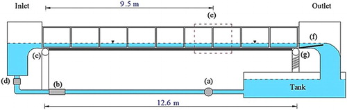
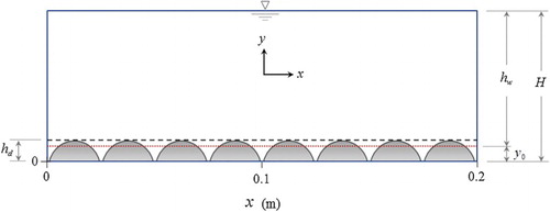
To validate the proposed SPH model, laboratory experiments of shallow turbulent open channel flow over a rough bed surface composed of regularly packed spheres were carried out. Measurements were taken from a 12.6 m long and 0.459 m wide rectangular open channel flume which included a pumped recirculation system, as shown in Fig. 4. The sidewalls of the flume were composed of glass. The measurement section was located 9.5 m from the inflow entrance, which given the maximum flow depth in the tests was considered to be long enough (> 100 flow depths) to ensure stable turbulent flow conditions had developed. To form a rough bed surface, the channel bottom was covered by two layers of spheres with diameter  = 25 mm and density of 1400 kg m⁻³, which were arranged in a hexagonal pattern. The channel bed slope was controlled by using an adjustable jack and uniform flow conditions were achieved by using an adjustable weir located at the outflow boundary. The flow rate was determined by using a calibrated orifice plate located inside the inlet pipe, and the depth-averaged flow velocity was determined from the measured flow rate and flow area. The vertical reference level was taken as the mean sphere elevation above the centreline of the upper sphere layer (4 mm below the top of the spheres), from which the flow depth was measured. Velocity measurements in the centre of the flume along the water column were taken by using a 3D side-looking acoustic Doppler velocimetry (ADV) probe, which was mounted on a scaled mechanical frame. For each single location, the velocity was measured using a sampling rate of 100 Hz and sampling period of 300 s. This sampling period was chosen so that it was long enough to provide time-converged velocity measurements. Throughout all of the measurements, the signal to noise ratio SNR and the signal correlation value were maintained at around 20 dB and 80%, respectively.

Figure 4 Side view of hydraulic flume: (a) pump; (b) orifice plate; (c) fixed pivot joint; (d) adjustable valve; (e) measurement section; (f) adjustable plate; and (g) adjustable jack

The temporal changes in the water surface elevations were measured using conductance wave probes. The wave probes consisted of two tinned copper wires of 0.25 mm in diameter, which were laterally separated by a distance of 13 mm and held under tension perpendicular to the water surface, such that they were partly submerged in the water. At the bottom of the flume, each probe was carefully attached to the spheres using strong glue, and the top of each probe was linked to a screw system enabling the wires to be vertically held under the tension without causing plastic deformation. An array of eight conductance wave probes was installed along the centreline of the flume in the measurement section. Figure 5 shows the top view of these eight probes labelled as WP1–WP8 and their relative streamwise positions.

Figure 5 The relative streamwise positions of the eight wave probes in the measurement section

All the probes were connected to wave monitoring modules provided by Churchill Controls (Crowthorne, Berkshire, UK). On the output of each wave monitoring module, a 10 Hz low-pass filter was used to eliminate the high frequency noise. All the wave probes were calibrated simultaneously and the procedure of this calibration was as follows. The flume was set to a slope of  = 0.0, and both the inlet and outlet ends were carefully blocked to ensure that no water could leak from the flume. The water in the tank was then pumped into the flume until a desired water depth was achieved. When the residual waves in the flume settled down (horizontal water surface), the voltage readings of the probes were recorded at 100 Hz for a period of 1800 s. This procedure was repeated for a number of flow depths ranging from 30 mm to 130 mm so that a linear relationship between the voltage and flow depth with a fit of a value of  = 0.99 was determined for each individual wave probe. This linear relationship was then used to convert the instantaneous voltage recorded on a wave probe into an accurate instantaneous water depth. The wave probes were regularly cleaned and calibrated before starting each measurement. During the calibration and measurement processes, the maximum change in the water temperature, which was measured by using a digital thermometer located beyond the measurement section, remained below 5.0%. A total of eight hydraulic flow conditions were created by using different water depths and bed slopes, which lead to a wide range of Froude Numbers as shown in Table 1. The experimental Reynolds Numbers ranged from approximately 10,000–40,000, so that all the flows are fully turbulent.

4 SPHysics simulations and results

4.1 Model set-up and computational parameters

Considering the numerical accuracy and the CPU load, the numerical flume was taken as 0.2 m long as shown in Fig. 6. The initial particle size was selected as 0.0015 m for all the flow conditions, giving a range of 4000–9000 particles involved in the model computation. The CFL stability number was taken as 0.15 and the computational time step was automatically adjusted to follow the Courant stability requirement (Gomez-Gesteira et al., 2012). In our numerical tests, it was found that a smoothing length of  = 1.5 provided the optimum results, including the water surface fluctuations. To determine the impact of varying the speed of sound for the SPH pressure equation, we made a series of sensitivity tests by using three different sound speed values as follows: (minimum value of as recommended by Monaghan & Kos, 1999), , and  = 60 m s⁻¹. It was found that a relatively large value of  = 60 m s⁻¹ was needed to be used for all the flow conditions to ensure stable flow for times up to 80 s–100 s. A realistic water viscosity ( =  m² s⁻¹) was used and the MLS filter was applied every 30 time steps to smooth out the density and pressure fluctuations. The MLS filter was chosen as it was found to provide better particle distributions throughout the flow depth as compared with the less computationally expensive Shepard filter.

Figure 6 Sketch of numerical flume with rough bed elements ( is bed roughness height = y₀ + 4 mm)

4.2 Velocity profiles and analysis

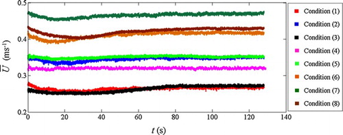
The SPH numerical model was run for each flow condition described in Table 1 until time exceeded 120.0 s. For each flow condition, the experimentally measured depth-averaged streamwise velocity listed in Table 1 was used as the input velocity of the fluid particles at the beginning of the computations. From the numerical observations, it was found that stable depth-averaged streamwise velocities were achieved after 100 s for the deeper flow conditions (6), (7) and (8), but earlier ( = 80 s) for the other shallower flow conditions (1)–(5), as shown in Fig. 7. This indicated that different initial input velocities can influence the timing of reaching the final steady state, but it has little effect on the final velocity values. Also an initial input velocity that was closer to the final stable value can make the evolution process quicker by using the present periodic boundary for the flow circulation. The computed data beyond a simulation time of 100 s were therefore unaffected by the initial model set-up, and were used in further analysis. To check this, the standard deviations of the time variation of depth-averaged velocities were calculated and the flow condition was considered to be stable when this value settled down to within ±2.0% of the standard deviation over 30 s. Therefore, all the following time-averaged streamwise velocities and shear stresses were computed over a period of 20 s after  = 100 s. This averaging period was found to be sufficiently long to obtain stable time-converged data.

Figure 7 Time variation of depth-averaged velocities vs. different initial inlet velocities

The streamwise velocity and shear stress at any point located at streamwise distance of and vertical distance of were computed by using the following two formulas: (17) (18) where we used a cubic spline kernel function to compute between the reference point and its neighbouring particle .

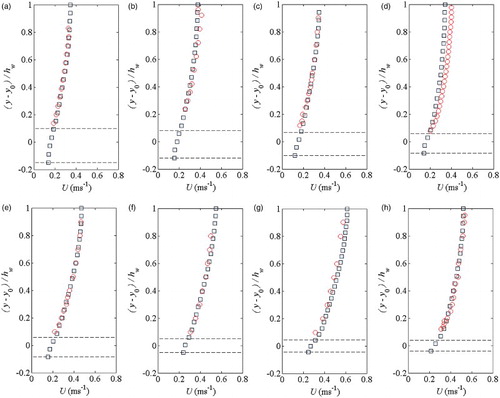
To validate the SPH computational results for the rough bed free surface turbulent flows, the computed time-averaged streamwise velocity profiles were compared with the experimental time-averaged measurements described in Section 3. The comparisons in Fig. 8 demonstrated a good agreement among the different data sets across the range of flow conditions. It is promising to note that these streamwise velocity profiles have been obtained without imposing any analytical solutions for the inflow or inner fluid regions, but rather they have evolved through the influence of the proposed drag force simulation and the turbulence model under the action of gravity in the SPH computations. To quantify the accuracy of SPH computations, the mean square error percentage (MSEP) between the numerical and experimental streamwise velocity profiles was calculated. We have found that the MSEP of the velocity profiles remained below 1.7% for all the flow conditions (1)–(8). On the other hand, relatively larger errors have been found in the velocity gradients. This was due to the kernel truncation error near the free surface and bed boundary, where the SPH velocity gradient was calculated, and also due to the experimental measurement errors. Nonetheless, the errors in the velocity gradient profiles stayed well below 16%.

Figure 8 Comparisons of time-averaged streamwise velocity profiles between experimental data and SPH results for (a) condition (1); (b) condition (2); (c) condition (3); (d) condition (4); (e) condition (5); (f) condition (6); (g) condition (7); and (h) condition (8) (circles: exp data; squares: SPH; dashed lines correspond to roughness top and bottom)

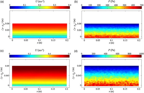
To demonstrate the variations of particle velocities of -component and pressure fields with respect to the flow depth, and also to check the stability of the numerical simulation, the time-averaged streamwise velocity and instantaneous pressure contours from the bottom of the spheres to the water surface were plotted in Fig. 9a and 9b, respectively, for the two flow conditions (3) and (7). In general, Fig. 9 reveals a systematic increase in the streamwise velocities through the flow depth. Although XSPH had been disabled in the model, the flow still developed in almost parallel layers, indicating that the fluid particles were quite uniformly distributed. This is due to the inclusion of the turbulence model and the drag force equation, which dampened the numerical noise in the particle field. The instantaneous pressure contours demonstrate an obvious deviation from the hydrostatic distribution due to the existence of turbulent flow structures. We can see that larger pressure fluctuations occurred in the regions just above the roughness top, where high turbulent intensities were expected to occur, as discussed later.

Figure 9 Contour maps of (a) time-averaged velocity; and (b) instantaneous pressure computed by SPH model for flow condition (3) and (c) time-averaged velocity; and (d) instantaneous pressure computed by SPH model for flow condition (7)

4.3 Shear stress profiles and analysis

Although a SPH modelling approach has been applied to a limited number of open channel free surface flows, there was almost no quantitative work reported on the time-averaged shear stress profiles due to a lack of an adequate closure model. Here the SPH computed shear stresses are compared with our experimental data, and the analytical solutions which were given by the following formula: (19) The experimental shear stresses were calculated from the velocity measurement data using the Reynolds stress as , where and are the streamwise and vertical fluctuating components obtained from the Reynolds decomposition as and , respectively. 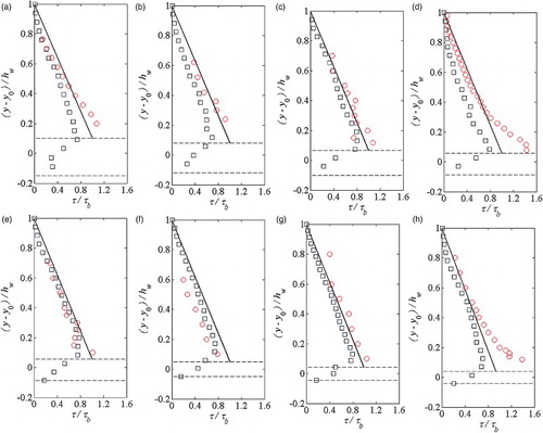The compared shear stresses were all normalized by the shear stress on the bed surface defined at the top of the roughness element and they are shown in Fig. 10. Although there were small errors found in the regions close to the channel bed due to the SPH kernel truncation errors and measurement uncertainties, the SPH predicted time-averaged shear stresses were in good agreement with the experimental data and the analytical solutions. It appeared that the contribution of the proposed drag force caused the largest flow velocity gradient to occur on the top of the roughness elements, which led to a maximum bed shear stress being slightly above the roughness top. We would expect that if a higher resolution were to be used, especially in the roughness interface (where the velocity gradient is high), a more accurate velocity gradient and shear stress would have been modelled. In comparison, the maximum shear stress computed by the “no drag force” model in a control run was found to be unreasonably located deep within the bed roughness element. It is also worth noting that some larger discrepancies were observed between the SPH results and experimental data for flow conditions (4) and (8) somewhere above the roughness crest. This could be attributed to the flow conditions in the laboratory experiment in which precise uniform flow conditions may not be achieved.

Figure 10 Comparisons of time-averaged shear stress profiles between experimental, analytical and SPH results for (a) condition (1); (b) condition (2); (c) condition (3); (d) condition (4); (e) condition (5); (f) condition (6); (g) condition (7); and (h) condition (8) (circles: exp data; squares: SPH; solid lines: analytical Eq. (19); dashed lines: roughness top and bottom)

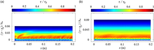
Furthermore, the time-averaged contour fields of the computed shear stress were plotted in Fig. 11 for the flow conditions (3) and (7), respectively, but over a slightly longer time period of 30 s after the simulation time  = 100 s. In general, the shear stress distributions revealed a gradual decrease towards the water surface, and the contour lines are continuous without obvious numerical noise. This provided the evidence that the SPH computations were stable and the numerical scheme was sound. Although the maximum velocity gradient occurs at the top of the spheres, the plots reveal that the maximum shear stress occurred at around 12–20% of the flow depth. This is due to the mixing length distribution used in the wall region () which dampens the near wall streamwise velocity gradient.

Figure 11 Time-averaged shear stress contours computed by SPH model for (a) conditions (3); and (b) condition (7)

4.4 Sensitivity analysis of model results

To check the convergence of the SPH computations and to evaluate the use of the mixing length model for the flow turbulence, the following two sensitivity tests were carried out.

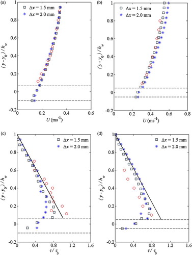
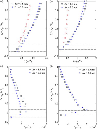
In Fig. 12a and 12b, we show the SPH computed flow velocity and shear stress profiles based on the mixing length model Eq. (12), for the two different particle spacings, i.e.  = 1.5 mm (original run) and 2.0 mm (new run), for the flow conditions (3) and (6), respectively. These two cases represented the relatively shallow and deep water conditions in our laboratory experiment. Both Fig. 12a and 12b showed generally good convergence behaviour in view of the overlapping of two SPH curves. However, there were some deviations in the two SPH shear stresses computed above the roughness crest region, especially for the shallow flow condition (3). The numerical results using a coarser particle spacing  = 2.0 mm generated smaller shear stress values here, although good overlapping behaviours have been observed for most of the flow region. We attributed this to the complexity in modelling shallow rough bed flows, in which a more stringent spatial resolution might be needed near the roughness elements to fully account for their effect on the flow.

Figure 12 Comparisons between experimental (red circles) and SPH (blue squares and stars) time-averaged velocity profiles for two different particle sizes for (a) condition (3); and (b) condition (6); Comparisons between experimental (red circles), analytical Eq. (19) (solid lines) and SPH (blue squares and stars) time-averaged shear stress profiles for two different particle sizes for (c) condition (3); and (d) condition (6)

Furthermore, another sensitivity test has been carried out to investigate the reason why the original SPS turbulence model of Gotoh et al. (2001) as represented by Eq. (10) could not provide satisfactory result in the present studies. In our investigations of the laboratory shallow open channel flows over a rough bed, the shear stresses computed from Eq. (10) were found to be much smaller than the experimental observations. This could be attributed to the fact that the computational particle size used in the model is much larger than many of the actual turbulence scales. Also, the coefficients of the SPS equation, such as , were commonly calibrated in the unsteady and transient flow applications, such as for a coastal wave, but it is not clear whether they can still perform well in a steady and long-time simulation of the open channel flows. In 2D uniform open channel flows, the velocity gradients of , and are almost zero when calculating the strain rate in Eq. (10), and the only dominant factor is , while all these values are quite large in coastal wave applications.

To numerically demonstrate this, the original SPS turbulence model predictions of the velocity and shear stress profiles for the two different particle sizes are shown in Fig. 13a and 13b, respectively, again for the shallower and deeper flow conditions (3) and (6). It is shown from Fig. 13a that due to insufficient turbulence dampening, the SPH computations predicted much faster flow velocities than the experimental data, although the two SPH velocities were almost converged, even for different particle sizes. On the other hand, Fig. 13b demonstrated that not only the turbulent shear stress values have been underestimated by several orders of magnitude as compared with Fig. 12b, but also the convergence degraded as well. This was due to the fact that the turbulent eddy viscosity in Eq. (10) is explicitly dependent on the particle size, so much more obvious discrepancies in the shear stress profiles appear around the roughness areas. In comparison, these differences were very small when the mixing length model of Eq. (12) is used, which is evidenced by the comparisons shown in Fig. 12b.

Figure 13 Comparisons between experimental (red circles) and SPH (blue squares and stars) time-averaged velocity profiles for two different particle sizes using original SPS turbulent model of Gotoh et al. (2001) for (a) condition (3); and (b) condition (6); Comparisons between SPH time-averaged shear stress profiles for two different particle sizes using original SPS turbulent model of Gotoh et al. (2001) for (c) condition (3); and (d) condition (6)

4.5 Turbulent intensity profiles

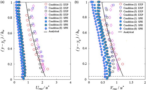
This section examines the performance of the proposed SPH model in predicting the turbulent flow intensities throughout the flow depth. The streamwise and vertical turbulent intensities were defined as the root-mean-square (rms) values of the turbulent velocity fluctuations at a particular point over a specific period, i.e. and . Figure 14a and 14b present the computed and measured turbulent intensity profiles for the flow conditions (1), (2), (5) and (8) listed in Table 1, for the streamwise and vertical quantities, respectively. The solid black lines in Fig. 14 are the analytical solutions proposed by Nezu and Nakagawa (1993) for turbulent free surface flows over a smooth bed as follows: (20) (21) It can be seen in Fig. 14 that the computed streamwise and vertical turbulent intensities appeared to decrease from the bed towards the free surface as observed in the laboratory measurements. This indicated that the proposed SPH model has the potential to simulate turbulent flow variations throughout the flow depth. However, the computed profiles were found to be much smaller in magnitude compared to the measured ones, which suggests that the model appeared to be unable to capture larger flow velocity fluctuations. One possible factor suppressing the magnitude of the computed turbulent flow structures could be the density filter applied in the current model. It would also be expected that larger velocity fluctuations could be computed if a much more refined computational particle size were to be used.

Figure 14 Normalized turbulent intensity profiles of (a) streamwise direction; and (b) vertical direction, for flow conditions (1), (2), (5) and (8) in Table 1 (dashed lines: roughness top)

4.6 Analysis of water surface fluctuations

Water surface identification and probability density function

Compared with the time-averaged water surface position in an open channel flow, the study of dynamic water surface behaviours would be more challenging. To identify the free surface, the divergence of particle positions can be used to compute the instantaneous water surface elevation at a desired streamwise location (Farhadi, Ershadi, Emdad, & Goshtasbi Rad, 2016; Lee et al., 2008). This divergence in the SPH formulation is defined as: (22) In 2D applications the divergence was equal to 2.0 when the kernel was fully supported (far away from the free surface boundary). Near the water surface the kernel was truncated due to the insufficient number of neighbouring particles, and thus the divergence becomes smaller than 2.0. This feature was used to identify the instantaneous water surface elevations. To determine which particle belonged to the water surface, a threshold value of 1.4, which gives the highest standard deviation of the water surface, was used in the present study. This value is also within the range 1.2–1.5 used by other SPH researchers (Farhadi et al., 2016; Lee et al., 2008).

In this work, the instantaneous water surface elevations at a desired streamwise location were computed as follows: first several vertical locations were defined below and above the initial water surface level by using a gauge spacing of  = 0.02 mm. At each of these locations, the particle divergence was computed every output time of 0.02 s, i.e. at a frequency of 50 Hz. Then the vertical location corresponding to the value closest to  = 1.4 was considered as the instantaneous water surface. This process was performed over a time period of 10.0 s, resulting in a total of 10/0.02 = 500 samples in the time series. This means that the flow has circulated more than 14 times throughout the numerical flume, which is believed to be sufficiently long to capture any spatial patterns on the free surface. Here the instantaneous water surface elevations were computed between the streamwise locations  = 0.02 m and  = 0.18 m using a gauge spacing 2.5 mm. By following this procedure, it was found that the maximum deviation between the measured and computed time-averaged water surface elevations occurs in flow condition (8) as presented in Table 2, and it remains below 5.0 mm, which is 5% of the uniform flow depth. It was also found that the probability density function (PDF) of the computed water surface fluctuations has a Gaussian distribution that agreed well with the experimental data as shown in Fig. 15, where the analysis was carried out for the flow conditions (1), (2), (5) and (8) as listed in Table 1. The solid red lines in Fig. 15 corresponded to the best fit of Gaussian probability density function, defined as , where is the water surface fluctuations and is the standard deviation. This finding also agrees well with the experimental observations reported by Horoshenkov et al. (2013) and Nichols, Tait, Horoshenkov, and Shepherd (2016) who measured the water surface fluctuations using conductance wave probes and laser induced fluorescence (LIF), respectively. However, we should note that the standard deviations of the computed water surface fluctuations were smaller compared with the experiments, and they do not appear to vary for the different flow conditions as listed in Table 2. This could be attributed to the limitation of the model in simulating large turbulent flow fluctuations as shown in the previous sections. Since the size of water surface fluctuations was believed to be dependent on the underlying turbulent flow structures, it was expected that the computed turbulent intensities would yield smaller water surface fluctuations.

Figure 15 Probability density functions of measured and computed water surface fluctuations for (a) conditions (1); (b) condition (2); (c) condition (5); and (d) condition (8) in Table 1

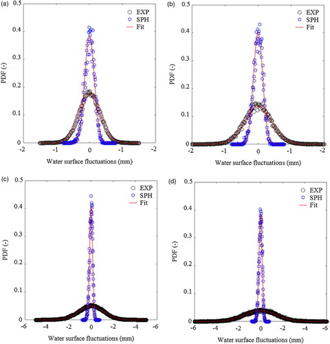
Table 2 Time-averaged water surface elevations and standard deviations of water surface fluctuation

Flow condition	(1)	(2)	(5)	(8)
Measured (mm)	39.00	49.00	72.00	104.00
Computed (mm)	40.00	49.70	69.20	99.00
Measured (mm)	0.32	0.40	1.15	1.50
Computed (mm)	0.15	0.14	0.14	0.15

Dynamic water surface pattern

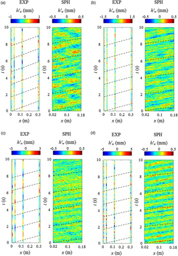
To investigate the dynamic behaviours of the water surface, the spatial-temporal field of the experimental and numerical instantaneous water surface fluctuations for flow conditions (1), (2), (5) and (8) were plotted in Fig. 16. The experimental plots showed the water surface fluctuations at the first four wave probes of WP1–WP4 located at 0.0, 0.028, 0.1203 and 0.3003 m, respectively. The black-dashed lines in Fig. 16 corresponded to the depth-averaged streamwise velocities listed in Table 1. The numerical plots demonstrated that the water surface is fluctuating between positive and negative elevations, travelling with almost the same orientation angle over space and time. This feature was more clearly captured in the shallow flow conditions (1) and (2) in Fig. 16, where the water surface pattern was more substantially influenced by the bed roughness. Despite the limited numbers of the measurement locations, the experimental dynamic features were also satisfactorily detected by the four streamwise probes and the patterns yield almost the same orientation angle. Although the numerical flume length is only 0.2 m due to the CPU constraint, the spatial period of the water surface oscillations agrees well with the result of Horoshenkov et al. (2013) and Nichols et al. (2016). It was possible to estimate the celerity of the water surface patterns in Fig. 16, and it was found that the gradient of these patterns approximately represents the depth-averaged flow velocity . Similar findings were reported in the experimental study of Fujita, Furutani, and Okanishi (2011), who showed that the water surface patterns travelled with a celerity close to the near-surface velocity. Here we should keep in mind that we used the SPH computational particle size of 1.5 mm, but the numerical model can capture flow information at a scale much more refined than this.

Figure 16 Comparisons of water surface dynamic patterns between experimental data and SPH results for (a) conditions (1); (b) condition (2); (c) condition (5); and (d) condition (8) in Table 1

Correlation characteristics of the water surface

As shown in the previous section, the water surface pattern is continuously changing over the time and space, so it was necessary to study its spatial dynamic behaviours in terms of the spatial correlation functions that could estimate the amplitude of the coherence and variance in water surface fluctuations at different locations. The measured and computed time-series of water surface fluctuations at different streamwise locations were cross-correlated to obtain the extreme value using the following equation: (23) where is the temporal cross-correlation function, () is the time-series data at streamwise locations (), separated by spatial streamwise distance , () is the time-averaged values, and is the time lag, corresponding to the time taken for the water surface wave to move between location and .

To examine the advection speed of the water surface pattern more accurately, the temporally normalized cross-correlation function was presented as a function of a spatial lag . For the experimental data, the first three probes WP1–WP3 were cross-correlated to give a number of four unique probe pairs as follows: WP1,1 ( = 0 mm), WP1,2 ( = 28 mm), WP2,3 ( = 92.3 mm), and WP1,3 ( = 120.3 mm). Meanwhile, for the SPH computations, more streamwise locations were cross-correlated to give nine unique streamwise spatial locations of  = 0.0, 7.5, 15.0, 22.5, 30.0, 37.5, 45.0, 52.5 and 60.0 mm, respectively. The results from the above procedures were plotted in Fig. 17, which showed the experimental and numerical temporal cross-correlation functions against the spatial lag for flow conditions (1), (2), (5) and (8). The red circles indicate the positions of the extreme values (maximum or minimum) of the experimental temporal cross-correlation function, whereas the blue squares represent the numerical ones.

Figure 17 Experimental (red circles) and SPH (blue squares) temporal cross-correlations for (a) conditions (1); (b) condition (2); (c) condition (5); and (d) condition (8) in Table 1

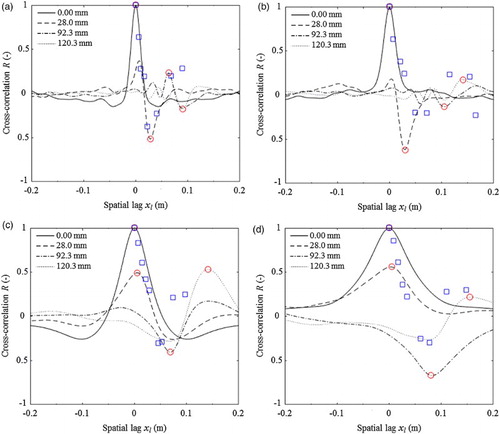
Horoshenkov et al. (2013) performed similar experimental studies and showed that the extreme values of the temporal cross-correlation between two streamwise locations occurred at a spatial lag of around . Similarly, the positions of the numerical SPH blue squares were also found to be very close to their streamwise spatial locations (Fig. 17). An interesting finding here is that both the experimental and numerical correlations demonstrate a similar form in that they start from the positive correlation of 1.0 and then flip their signs at a certain spatial lag . As this spatial lag further increased, their correlations become positive again and approach a value smaller than 1.0. This agreed well with the experimental results of Nichols et al. (2016), where the physical mechanisms behind the change of the sign were discussed. The results in Figs 16 and 17 could provide strong evidence that the SPH model was able to simulate the spatial and temporal patterns of the dynamic free surface although the accuracy of predicting the instantaneous extreme elevation values is limited by the particle resolution and the applied density filter.

5 Conclusions

This paper reported on the use of the SPH method for the simulation of shallow turbulent free surface flows over rough beds. Eight flow conditions have been studied through laboratory experiments carried out in a flume with a rough bed being composed of uniformly sized spheres placed in a regular hexagonal pattern. For each flow condition, the velocity measurements recorded vertically along the water column were taken at the centreline of the flume using 3D side-looking ADV. Also the instantaneous water surface elevations at different streamwise locations were recorded for four flow conditions. The numerical SPH model was modified with a turbulent closure based on the mixing length approach, and a drag force term was added into the momentum equation to account for the rough boundary.

We found that the improved model could provide an adequate solution to simulate the time-averaged quantities for shallow turbulent free surface flows over a rough boundary. The sensitivity tests using different particle spacings and turbulent closure techniques revealed that the original SPS turbulent model with a fixed Smagorinsky constant predicted much smaller and inconsistent shear stresses as compared with the experimental observations, while our proposed model using a mixing length approach could predict well the measured time-averaged shear stress profiles. The numerical model was also shown to be capable of simulating the depth-wise variation of turbulent intensities and the spatial patterns of water surface fluctuations. It was found that the predicted advection speed of water surface patterns is very close to the mean bulk flow velocity. This corresponded with the experimental observations. Besides, a similarity was also found between the experimental and SPH spatial correlations of the water surface fluctuations.

The strength of the study lies in that a standard SPS model has been improved by replacing the fixed Smagorinsky constant with a mixing length formulation that does not require a tuning parameter. This improvement is straightforward to implement and introduces the dependency from both the local flow conditions and size of the flow structures in order to obtain better representation of the streamwise flow velocity and shear stress profiles even using a particle resolution that is lower than the actual turbulence scales. In addition, the drag force exerted on the flow by the roughness elements at the channel bed is simulated in the SPH model by introducing an equivalent drag force term in the momentum balance equation, and the roughness scale is treated as a dynamic parameter, depending not only on the absolute value of the bed grain size but also on the related flow depth. The above modifications have been successfully implemented on an open source code (SPHysics) that is easily accessible and could become an interesting engineering tool for the analysis of free surface turbulent flows, including the spatial patterns of the velocity and water surface behaviours.

However, it should be realized that the SPH implementation has difficulties in predicting some more subtle features of the turbulent flow structures, such as its spectrum, and thus the turbulent fluctuations of the free surface can be expected to be poorly predicted. This is illustrated by the computational results that show the insensitivity of the model regarding the fluctuations of the free surface for the flow conditions, while the experimental results clearly indicate such an influence. In general we found that the present model is better at simulating time-averaged flow quantities but needs further improvement to accurately reproduce the larger instantaneous values of velocity. The reason is that SPH is fundamentally a dissipative numerical method which uses kernel averaging to calculate fluid quantities and this could smooth out the characteristics of real physical fluctuations. The use of a density filter in WCSPH to deal with the numerical noise could also impact on the simulation of turbulent velocity fluctuations. Finally, the current method of modelling the fluid drag force may not simulate the flow dispersion correctly near the bed and a more advanced treatment of the bed roughness could help to improve the prediction of instantaneous velocities.

The SPH numerical simulations have been performed on a PC with an Intel® Core(TM) i7-4770 CPU 3.4 GHz and 32.0 GB of RAM running a 64-bit version of windows. The total CPU time required for one single flow condition ranged from 7–15 days from the shallow to deep flow conditions. In future studies, the engineering value of the proposed model could be further enhanced by extending it to the analysis of similar problems with a deformable bed and comparing the results with other SPH models for fluid–grain interactions. Also the influence of surface tension force should be addressed in follow-on modelling work.

Notation

	=	reference area of bed roughness element (m2)
	=	coefficient in equation of state (–)
	=	coefficient in Log-Law equation (–)
	=	speed of sound at reference density (m s−1)
	=	drag coefficient (–)
	=	coefficient in SPS turbulent equation (–)
	=	Smagorinsky constant (–)
	=	diameter of bed roughness sphere (m)
	=	Froude Number (–)
	=	bed drag force (N)
	=	gravitational acceleration vector (m s−2)
	=	kernel smoothing length (m)
	=	bed roughness height (m)
	=	instantaneous water depth at streamwise location (m)
	=	time-averaged water depth (m)
	=	water surface fluctuation (m)
	=	total flow depth (m)
	=	turbulent kinetic energy (s−1)
	=	hydraulic roughness (m)
	=	mixing length (m)
	=	half-chord length of bed roughness sphere (m)
	=	particle mass (kg)
	=	particle pressure (Pa)
	=	Probability density function (–)
	=	radius of bed roughness sphere (m)
	=	particle position vector (m)
	=	Reynolds Number (–)
	=	temporal cross-correlation function (–)
	=	local strain rate (s−1)
	=	channel bed slope (–)
	=	SPS strain component (s−1)
	=	time (s)
	=	particle velocity vector (m s−1)
	=	instantaneous streamwise velocity (m s−1)
	=	streamwise fluctuating velocity (m s−1)
	=	shear velocity (m s−1)
	=	time-averaged streamwise velocity (m s−1)
	=	depth-averaged streamwise velocity (m s−1)
	=	reference velocity on bed roughness element (m s−1)
	=	root-mean-square of streamwise turbulent velocity fluctuations (m s−1)
	=	instantaneous vertical velocity (m s−1)
	=	vertical fluctuating velocity (m s−1)
	=	time-averaged vertical velocity (m s−1)
	=	root-mean-square of vertical turbulent velocity fluctuations (m s−1)
	=	kernel function (m−2)
	=	streamwise distance (m)
	=	streamwise spatial lag (m)
	=	vertical distance (m)
	=	experimental datum (m)
	=	polytrophic coefficient in equation of state (–)
	=	Kronecker’s delta (–)
	=	particle spacing (m)
	=	gauge spacing (m)
	=	XSPH coefficient (–)
	=	von Kármán constant (–)
	=	constant in mixing length equation (–)
	=	kinematic viscosity (m2 s−1)
	=	turbulent eddy viscosity (m2 s−1)
	=	fluid density (kg m−3)
	=	reference density (kg m−3)
	=	spatial streamwise lag distance in water surface correlation relationship (m)
	=	standard deviation of water surface fluctuations (m)
	=	turbulent shear stress tensor (Pa)
	=	shear stress on bed (Pa)
	=	SPS shear stress component (Pa)
	=	time lag (s)

Acknowledgements

We are very grateful to Dr Huaxing Liu, Maritime Research Centre of Nanyang Technological University, Singapore for his invaluable guidance on the initial coding work. Special thanks also go to Prof Vladimir Nikora (outgoing Editor) who kindly made editorial revisions on the manuscript.

Additional information

Funding

Author E. Gabreil would like to acknowledge the financial support provided by the Libyan Ministry of Higher Education for his four years of PhD study. The experimental work was supported by EPSRC [grant EP/G015341/1]. Author S. Shao would like to acknowledge the National Key Basic Research Program (973 program) of China [grant 2013CB036402].

References

- Blinco, P. H., & Partheniades, E. (1971). Turbulence characteristics in free surface flows over smooth and rough boundaries. Journal of Hydraulic Research, 9, 43–71. doi: 10.1080/00221687109500337
- Chern, M.-J., & Syamsuri, S. (2013). Effect of corrugated bed on hydraulic jump characteristic using SPH method. Journal of Hydraulic Engineering, 139, 221–232. doi: 10.1061/(ASCE)HY.1943-7900.0000618
- Colagrossi, A., & Landrini, M. (2003). Numerical simulation of interfacial flows by smoothed particle hydrodynamics. Journal of Computational Physics, 191, 448–475. doi: 10.1016/S0021-9991(03)00324-3
- Dalrymple, R. A., & Knio, O. (2001, June). SPH modelling of water waves. In H. Hanson & M. Larson (Eds.), Proceedings of 4th international conference on coastal dynamics (pp. 779–787). Lund: ASCE.
- Dalrymple, R. A., & Rogers, B. D. (2006). Numerical modeling of water waves with the SPH method. Coastal Engineering, 53, 141–147. doi: 10.1016/j.coastaleng.2005.10.004
- De Padova, D., Mossa, M., Sibilla, S., & Torti, E. (2013). 3D SPH modelling of hydraulic jump in a very large channel. Journal of Hydraulic Research, 51, 158–173. doi: 10.1080/00221686.2012.736883
- Džebo, E., Žagar, D., Krzyk, M., Četina, M., & Petkovšek, G. (2014). Different ways of defining wall shear in smoothed particle hydrodynamics simulations of a dam-break wave. Journal of Hydraulic Research, 52, 453–464. doi: 10.1080/00221686.2013.879611
- Einstein, H. A., & El-Samni, E. A. (1949). Hydrodynamic forces on a rough wall. Reviews of Modern Physics, 21, 520–524. doi: 10.1103/RevModPhys.21.520
- Farhadi, A., Ershadi, H., Emdad, H., & Goshtasbi Rad, E. (2016). Comparative study on the accuracy of solitary wave generations in an ISPH-based numerical wave flume. Applied Ocean Research, 54, 115–136. doi: 10.1016/j.apor.2015.11.003
- Federico, I., Marrone, S., Colagrossi, A., Aristodemo, F., & Antuono, M. (2012). Simulating 2D open-channel flows through an SPH model. European Journal of Mechanics – B/Fluids, 34, 35–46. doi: 10.1016/j.euromechflu.2012.02.002
- Fujita, I., Furutani, Y., & Okanishi, T. (2011). Advection features of water surface profile in turbulent open-channel flow with hemisphere roughness elements. Visualization of Mechanical Processes: An International Online Journal, 1(4), paper no. 1. doi: 10.1615/VisMechProc.v1.i3.70
- Gingold, R. A., & Monaghan, J. J. (1977). Smoothed particle hydrodynamics: theory and application to non-spherical stars. Monthly Notices of the Royal Astronomical Society, 181, 375–389. doi: 10.1093/mnras/181.3.375
- Gómez-Gesteira, M., & Dalrymple, R. A. (2004). Using a three-dimensional smoothed particle hydrodynamics method for wave impact on a tall structure. Journal of Waterway, Port, Coastal, and Ocean Engineering, 130, 63–69. doi: 10.1061/(ASCE)0733-950X(2004)130:2(63)
- Gomez-Gesteira, M., Rogers, B. D., Crespo, A. J. C., Dalrymple, R. A., Narayanaswamy, M., & Dominguez, J. M. (2012). SPHysics – development of a free-surface fluid solver – Part 1: Theory and formulations. Computers and Geosciences, 48, 289–299. doi: 10.1016/j.cageo.2012.02.029
- Gotoh, H., & Sakai, T. (1999). Lagrangian simulation of breaking waves using particle method. Coastal Engineering Journal, 41, 303–326. doi: 10.1142/S0578563499000188
- Gotoh, H., Shibahara, T., & Sakai, T. (2001). Sub-Particle-Scale turbulence model for the MPS method – Lagrangian flow model for hydraulic engineering. Computational Fluid Dynamics Journal, 9, 339–347.
- Horoshenkov, K. V., Nichols, A., Tait, S. J., & Maximov, G. A. (2013). The pattern of surface waves in a shallow free surface flow. Journal of Geophysical Research: Earth Surface, 118, 1864–1876.
- Hu, X. Y., & Adams, N. A. (2007). An incompressible multi-phase SPH method. Journal of Computational Physics, 227, 264–278. doi: 10.1016/j.jcp.2007.07.013
- Kamphuis, J. W. (1974). Determination of sand roughness for fixed beds. Journal of Hydraulic Research, 12, 193–203. doi: 10.1080/00221687409499737
- Khayyer, A., & Gotoh, H. (2010). On particle-based simulation of a dam break over a wet bed. Journal of Hydraulic Research, 48, 238–249. doi: 10.1080/00221681003726361
- Kumar, S., Gupta, R., & Banerjee, S. (1998). An experimental investigation of the characteristics of free-surface turbulence in channel flow. Physics of Fluids, 10, 437–456. doi: 10.1063/1.869573
- Lee, E.-S., Moulinec, C., Xu, R., Violeau, D., Laurence, D., & Stansby, P. (2008). Comparisons of weakly compressible and truly incompressible algorithms for the SPH mesh free particle method. Journal of Computational Physics, 227, 8417–8436. doi: 10.1016/j.jcp.2008.06.005
- López, D., Marivela, R., & Garrote, L. (2010). Smoothed particle hydrodynamics model applied to hydraulic structures: A hydraulic jump test case. Journal of Hydraulic Research, 48(SI), 142–158. doi: 10.1080/00221686.2010.9641255
- Meister, M., Burger, G., & Rauch, W. (2014). On the Reynolds number sensitivity of smoothed particle hydrodynamics. Journal of Hydraulic Research, 52, 824–835. doi: 10.1080/00221686.2014.932855
- Monaghan, J. J., & Kos, A. (1999). Solitary waves on a Cretan beach. Journal of Waterway, Port, Coastal, and Ocean Engineering, 125, 145–155. doi: 10.1061/(ASCE)0733-950X(1999)125:3(145)
- Nakagawa, H., Nezu, I., & Ueda, H. (1975). Turbulence of open channel flow over smooth and rough beds. Proceedings of the Japan Society of Civil Engineers, 1975, 155–168. doi: 10.2208/jscej1969.1975.241_155
- Nezu, I., & Nakagawa, H. (1993). Turbulence in open-channel flows [IAHR Monograph]. Rotterdam: Balkema.
- Nichols, A., Tait, S. J., Horoshenkov, K. V., & Shepherd, S. J. (2016). A model of the free surface dynamics of shallow turbulent flows. Journal of Hydraulic Research, 54, 516–526. doi: 10.1080/00221686.2016.1176607
- Schmeeckle, M. W., Nelson, J. M., & Shreve, R. L. (2007). Forces on stationary particles in near-bed turbulent flows. Journal of Geophysical Research: Earth Surface, 112, F02003. doi: 10.1029/2006JF000536
- Shakibaeinia, A., & Jin, Y. C. (2010). A weakly compressible MPS method for modeling of open-boundary free surface flow. International Journal for Numerical Methods in Fluids, 63, 1208–1232.
- Smolentsev, S., & Miraghaie, R. (2005). Study of a free surface in open-channel water flows in the regime from “weak” to “strong” turbulence. International Journal of Multiphase Flow, 31, 921–939. doi: 10.1016/j.ijmultiphaseflow.2005.05.008
- Stansby, P. K. (2003). A mixing-length model for shallow turbulent wakes. Journal of Fluid Mechanics, 495, 369–384. doi: 10.1017/S0022112003006384
- Violeau, D., & Issa, R. (2007). Numerical modelling of complex turbulent free-surface flows with the SPH method: an overview. International Journal for Numerical Methods in Fluids, 53, 277–304. doi: 10.1002/fld.1292