Implications of the selection of a particular modal decomposition technique for the analysis of shallow flows

ABSTRACT

This work deals with the capabilities of two synoptic modal decomposition techniques for the identification of the spatial patterns and temporal dynamics of coherent structures in shallow flows. Using two different experimental datasets it is shown that due to the linear behaviour of large-scale, quasi-two-dimensional flow structures, there are almost no differences in the identification of dominant modes between the results obtained from a traditional proper orthogonal decomposition and the more recently developed dynamic mode decomposition. However, it is also shown that nonlinear dynamics can arise in the transition of these structures to a quasi-two-dimensional behaviour, which can result in the proper orthogonal decomposition identifying structures composed of multi-frequencies, a sign of a convoluted dynamics. Thus dynamic mode decomposition is recommended instead for the analysis of such phenomena. In addition, this paper introduces a simple ranking methodology for the use of the dynamic mode decomposition technique in shallow flows, which is based on the results of the proper orthogonal decomposition.

Keywords:

• Coherent structures
• dynamic mode decomposition (DMD)
• particle image velocimetry (PIV)
• proper orthogonal decomposition (POD)
• quasi-two-dimensional coherent structures (Q2DCS)
• shallow flows

1. Introduction

The main effect caused by the forcing of a topographical obstruction in a turbulent shallow flow is the generation of highly energetic coherent structures (Jirka, 2001). Due to the constraints imposed by the water depth on the vertical vortex stretching process, these coherent structures grow sidewise, developing mainly horizontal dynamics. This means that their structure is almost two-dimensional everywhere on depth, except near the bottom where the boundary layer governs the flow characteristics, i.e. they behave as quasi-two-dimensional coherent structures (Q2DCS) (Jirka & Uijttewaal, 2004). Besides the Reynolds number, Q2DCS are mainly characterized by the shallowness number , where is the friction coefficient, D a characteristics length scale and H the water depth (Chen & Jirka, 1997; Uijttewaal, 2014; Constantinescu et al., 2009). Due to the high energy of Q2DCS, their dynamics can be crucial to understand important process such as momentum and mass exchange, and the dynamic loads exerted by a flow over hydraulics infrastructure. It is because of this that the description of their spatial characteristics and temporal dynamics is paramount in the context of environmental process and hydraulic engineering.

There are several techniques that can be used to generate synoptic data to investigate the behaviour of topographically forced shallow flows. These can include data gathered from field or laboratory image-based velocimetry measurements (Weitbrecht et al., 2002; Uijttewaal & Jirka, 2003), or those generated by numerical eddy resolving techniques (Hinterberger et al., 2007; Rodi, 2017). It is in the context of these large datasets where the selection of tools for the identification of statistically meaningful coherent structure can play an important role.

From a general perspective, modal decomposition techniques can be used to determine regions of dynamical and spatial significance (Lumley et al., 1996) from large datasets. A popular modal decomposition technique is proper orthogonal decomposition (POD) (Aubry, 1991; Berkooz et al., 1993). This technique is used to find a set of spatially orthogonal modes which are ordered by their contribution to the total variance, i.e. turbulent kinetic energy in the case of velocity time series, or enstrophy in case of vorticity fields. Previous research has shown the POD to be an effective method in describing complex processes in open channel flows (Roussinova et al., 2010; Fox & Belcher, 2011; Higham & Brevis, 2018) and in the context of shallow flows (Brevis & García-Villalba, 2011; Peltier et al., 2014).

An alternative to POD, the dynamic mode decomposition (DMD) (Schmid et al., 2009) has been introduced relatively recently. The main difference with POD is that the method searches for temporally orthogonal modes. DMD has been successfully applied to a number of experimental cases, but its application has been mainly limited to a range of problems in fluid mechanics (Schmid et al., 2009; Muld et al., 2012; Tu et al., 2013). Even though both techniques have offered insights into complex systems and processes, it is necessary to understand some of their limitations to avoid any misinterpretation of the physical insights they offer.

POD is a linear statistical method and as a consequence assumes that modes can be superimposed for the reconstruction of the signal. This means that complex nonlinear cases can cause the low-order POD modes to be convolved with multiple, high variance, contributing mechanisms. As the DMD algorithm extracts spatial modes which are temporally orthogonal, the structures described in the modes relate only to discrete frequencies, thus are unlikely to describe multiple mechanisms. However, the extracted modes cannot be related directly to a physical quantity such a enstrophy or kinetic energy, making it difficult to pinpoint the meaning of the modes in terms of the types of physics that are often used to inform process insight or numerical modelling. A number of previous works have aimed to solve this problem usingoptimization techniques (Jovanović et al., 2014), or modal reductions (Chen et al., 2012; Wynn et al., 2013). In this work a simple alternative to these methods is presented, with a particular application to the use of the DMD technique for the analysis of Q2DCS in shallow dynamics. Based on the mainly linear, or weakly nonlinear, behaviour of large Q2DCS in shallow flows for low values of the shallowness number (Ghidaoui et al., 2006), POD should offer a good performance for the identification of coherent structures. However for larger or in the region of transition of these structures to a quasi two-dimensional behaviour, the flow patterns can be affected by three-dimensional structures, thus producing a departure from a linear behaviour. Even though POD cannot capture the full nature of the modes under these conditions, it can be expected that due to the still dominant two-dimensionality of the flow, the results will contain enough information on the dominant dynamics. As explained later in detail, this information can be found in the temporal coefficients resulting from a POD, which, after a Fourier spectral analysis, can guide the search for corresponding modes using the DMD technique. Thus, the aim of this paper is to not only to demonstrate the potential utility of DMD in hydraulics research, but also to show how it can be complemented, and the interpretation of its results enhanced, through the use of information from POD. Overviews of these two techniques are provided in the next two sections, with further detail available in the literature. Results where DMD and POD largely return the same behaviours are then presented, before considering a case in greater detail where more complex flow dynamics requires the use of the two techniques in parallel.

2. Proper orthogonal decomposition

POD was independently derived by a number of individuals, and consequently takes a variety of names in different fields such as Karhunen–Loève decomposition, singular value decomposition (SVD) and principal components analysis (PCA) (Kosambi, 1943; Loève, 1945; Karhunen, 1946; Pougachev, 1953; Obukbov, 1954). A set of temporally ordered velocity/vorticity fields, , is considered, each of which is of size . The method requires the construction of an matrix from T columns of length N=XY , each one corresponding to a column-vector version of a transformed snapshot . A POD can be obtained by: (1) where is a matrix of size (Ω are the number of modes of the decomposition and represents a conjugate transpose matrix operation). is the vector containing the contribution to the total variance of each Ω. The elements in are ordered in descending rank order, i.e. (). In practical terms the matrix of size contains the spatial structure of each of the modes and the matrix of size contains the coefficients representing the time evolution of the modes.

From Eq. (1(1) ) and as shown by Brevis and García-Villalba (2011), each relates to the temporal evolution of each , where . As outlined above, each POD mode is spatially orthogonal and may contain multiple intertwined mechanisms; therefore a Fourier spectrum of each should be able to highlight the peak frequencies relating to these intertwined periodicities.

3. Dynamic mode decomposition

The dynamic mode decomposition (DMD) algorithm was introduced by Schmid (2010), based on a Arnoldi eigenvalue algorithm suggested by Ruhe (1984). The DMD algorithm approximates the temporal dynamics by fitting a high-degree polynomial to a Krylov sequence of flow fields (Mezić, 2005; Schmid et al., 2009). For complex flow systems containing interactions of turbulent structures and mechanisms, the DMD algorithm can be used to extract spatial modes with single ‘pure’ frequencies. There are a number of methods to compute a DMD, and that implemented in the present study is the popular SVD-based algorithm, which is used to reduce the susceptibility to experimental noise, through an initial projection on to a orthogonal basis (Schmid, 2010). The algorithm is outlined below, although the reader is directed to Schmid (2010), Jovanović et al. (2014) and Tu et al. (2013) for the full mathematical description. The DMD algorithm begins with a similar transformation as POD, with the difference that two matrices are formed that are each one column smaller than the full dataset; the idea is to use the former as a means to predict the data in the latter: (2) where , and the super-scripts A and B denote the two matrices of size . A SVD of is computed, such that: (3) where , and are the POD modes, the singular values and the temporal coefficients of respectively, and where ∼ relates to the SVD quantities in the DMD algorithm. The matrix , of size , is created by: (4) and its complex eigenvalues, , and eigenvectors, , are computed where . At this point the method of Jovanović et al. (2014) is used, as this creates a set of amplitudes for each spatial mode. Following Jovanović et al. (2014) a Vandermonde matrix is created from the complex eigenvalues: (5) where and , and the spatial modes are created by , where is the set of complex eigenvectors previously computed. Furthermore, a set of amplitudes, , are created and the original input, , can be expressed as: (6) where is of size . Similar to a POD , the spatial are modes of size relating to the spatial structure, relates to their amplitude , but not their variance, and contains the coefficients representing the time evolution of the modes. In practical terms, the angle between the real and imaginary part of, , can be used to describe the frequency, f, relating to each and can be expressed by: (7) From Eq. (7(7) ), it is clear that each of the modes obtained by DMD relates to a unique peak frequency. If the Fourier spectrum of the POD coefficients is used to identify the frequency of dominant but intertwined structures, these frequencies can be used to identify their spatial structure from the DMD results. There is a main restriction for this methodology. The technique can be applied only for the identification of low order modes in shallow flows or in cases where a flow structure clearly governs the dynamics. In these flows, peak frequencies are expected to be clearly identified from the Fourier spectrum of the temporal POD coefficients. These conditions do not hold, for instance, in three-dimensional turbulent flows, where the contribution of low order modes can be of a similar magnitude to the contribution of higher order ones. Thus, any frequency extracted from the Fourier spectrum might be misleading due to the lack of capabilities of POD, being spatially orthogonal, to separate nonlinear interactions of structures with similar contributions to the variance of the signal. It is because of this that the link between POD and DMD introduced here, is only presented in the context of shallow flows. Furthermore, a recent contribution by Taira et al. (2017) also shows that DMD is not suitable for complex highly anisotropic flows, therefore the use of DMD for shallow quasi-two dimensional flows seems most logical.

4. Flow visualizations of a shallow cylinder wake

A first experimental dataset was selected to showcase hydrodynamic conditions where the DMD does not improve the identification of Q2DCS in the low order modes, obtained by POD. The dataset was obtained from the experimental work of Brevis and García-Villalba (2011), in which the POD of a flow visualization was used to identify dominant frequencies in the wake of a cylinder in a shallow flow. All experimental details can be found in the work of Brevis & García-Villalba (2011). Figure 1 shows the results obtained from the POD analysis. In this case the spatial modes are paired, indicating a periodic shedding behaviour with a different phase in these two modes. Figure 1a only shows as reference. The modes in Fig. 1a and b reveal the advection of patches of dye transported by vortical structures. Modes (Fig. 1c and d), are also paired but show a different structure. According to Brevis and García-Villalba (2011) these modes correspond to the spanwise alternated motion of the vortex behind the cylinder. Figure 1e and f show the evolution of the temporal coefficients is clearly sinusoidal; consequently a peak at can be observed in the Fourier power spectra for modes and . Due to the size of the region analysed, it is expected that the Q2DCS will govern most for the spatial flow features. 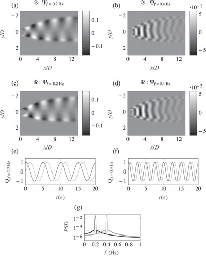In addition , thus it is expected to see a highly linear dynamic of the dominant modes. This can be seen in Fig. 2a–d where the results of the DMD analysis are given; the spatial structure of the modes is very similar to that obtained by the POD. However, different to the POD analysis, in the DMD spatial modes the advection of the patches of the transported dye can be seen between the real and imaginary components of the spatial modes. As shown in Fig. 2e and f in both cases the coefficients show a sinusoidal shape, although noticeably there is a sharper peak in the Fourier spectra in Fig. 2g, highlighting the better localization of the DMD method.

Figure 1. POD results of flow visualizations of a shallow cylinder wake. (a–d) The spatial modes . (e, f) The temporal coefficients and in black and and in grey. (g) Fourier power spectrum of the temporal coefficients (black) and (grey). The red dashed lines highlight the frequencies extracted using the DMD

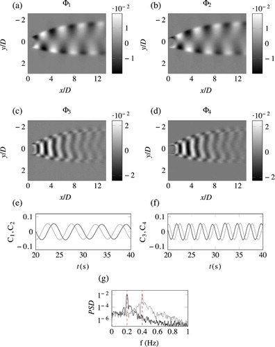
Figure 2. DMD results of flow visualizations of a shallow cylinder wake. (a–d) The real and imaginary components of the spatial modes and respectively. (e, f) The real and imaginary temporal coefficients relating to and where the black line is the real component and the grey line is the imaginary component. (g) The Fourier power spectra of the temporal coefficients shown in (e) and (f). (black) and (grey)

5. Shallow flow obstructed by a groyne

A shallow turbulent flow obstructed by a single groyne is a common occurrence in fluvial shallow flow hydraulics. The selected case corresponds to a flow topology similar to the one described by Talstra (2011). The flow that developed downstream of the obstacle is characterized by the formation of a shear layer bounding a low velocity recirculation region formed by a primary clockwise gyre, located in the downstream part of the recirculation zone, and an anti-clockwise secondary gyre, of smaller size, located immediately downstream the obstacle. The structures populating the shear layer in the near field are expected to be generated by both vortex shedding from the tip of the obstacle and by the strong velocity gradient produced between the main channel and the secondary gyre interface. From a general observation of the derived vorticity fields sequence, it is expected that the vortices associated with the velocity gradient are of a larger size as the mechanism of generation seems to be more energetic than vortex shedding. Even though , the region analysed here is the near field, where vortices are not expected to behave as a Q2DCS, but are in a transitional stage, still governed by quasi two-dimensional features, but also influenced by three-dimensional ones.

The dataset in the present study is a subset of the data presented in (Higham, Brevis, Keylock, & Safarzadeh, 2017). The experiments were carried out in a tilting shallow flume of located at the Institute for Hydromechanics, Karlsruhe Institute of Technology, Germany. A single rectangular obstacle of length D=0.25 m and cross section  m was placed perpendicular to the main flow direction, at the side-wall of the flume, and at 12 m downstream from the channel entrance. The flow rate Q was set to 0.0135 m³s⁻¹, and the flume slope was inclined to 0.001 m m⁻¹ resulting in a water depth H=0.04 m (see Fig. 3). The Reynolds number was, , where , ρ and ν are the bulk flow velocity, water density and kinematic viscosity respectively. These conditions gave a low Froude number, , where g is the acceleration of gravity, which ensured minimal surface disturbances (Uijttewaal, 2005). The friction factor was estimated to be 0.03, thus . The dynamic of the Q2CS was quantified by means of large scale particle image velocimetry (LSPIV) measurement. The PIV system consisted of a camera with a pixel CCD-sensor and 12 bit resolution. The flow was seeded with floating 2.5 mm particles using a pneumatic particle dispenser. It has been previously shown that the use of these tracer particles is effective in capturing the large scale turbulent motions (Weitbrecht et al., 2002). The camera was mounted directly above the water surface at a height of 1.5 m and was set to capture an area of  m downstream of the obstacle. A total of 700 snapshots were recorded with an acquisition frequency of 7.5 Hz. The image sequence was analysed using the PIV lab (Thielicke & Stamhuis, 2014), using multi-pass and image deformation techniques (Scarano, 2002), and the raw PIV results were filtered using the PODDEM algorithm (Higham, Brevis, & Keylock, 2016).

Figure 3. Illustration of the experimental set-up of the single groyne. Measurement section highlighted in white. (Not to scale.)

Both the POD and DMD calculations were undertaken on all 700 snapshots. The POD was calculated over the snapshots of the fluctuating velocity field, while the DMD was performed over the instantaneous velocity snapshots. The reasoning behind this is related to the stability of the DMD solution, as discussed by Tu et al. (2013) and Chen et al. (2012).

In Fig. 4b and c the first two POD modes, , of the vorticity field are presented. These top two spatial modes have similar energy, contributing to ∼35% of the total variance. As shown by Rempfer and Fasel (1994) and Brevis and García-Villalba (2011), two modes of similar energy can show analogous, but shifted, spatial and temporal features. In this particular case, these shifted features appear to be related, as expected, to the advection of vortices resulting from a Kelvin–Helmholtz instability.

Figure 4. POD results of the near vorticity field of the shear layer generated by a lateral groyne in a shallow flow (groyne highlighted in white). (a) The time averaged vorticity field . (b, c) The POD spatial modes, and . (d, e) The POD temporal coefficients of and respectively, where the grey line denotes the mode which forms the conjugate pair. (f) The Fourier power spectra of the temporal coefficients shown in (d) and (e). (black) and (grey). The red dashed lines highlight the frequencies of importance; extracted using the DMD

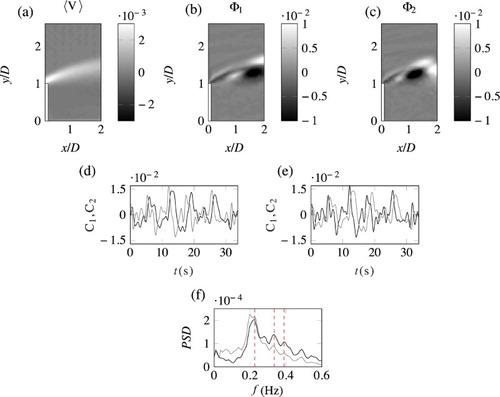
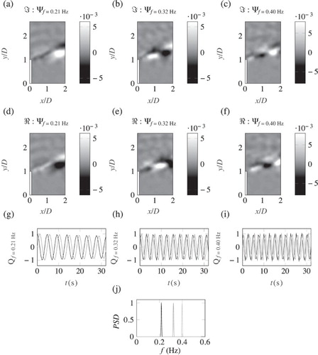
In Fig. 4d and e the temporal coefficients, , of the first two modes are presented. The evolution of the coefficients appears to correspond to the presence of multiple dynamical processes. This is further revealed by the Fourier spectrum of (see Fig. 4f), which shows the presence of a broad band of frequencies but with clear peaks, at different energy levels, and frequencies of . After performing the DMD analysis on the data, the modes associated to these peak frequencies were identified. The imaginary components of the DMD spatial modes are shown in Fig. 5a–c and the real components in Fig. 5d–f. The temporal coefficients relating to these modes are presented in Fig. 5g–i where the black lines are the real components and the grey lines are the imaginary components. Figure 5j highlights how sharply the identified frequencies are expressed in the DMD modes. In Fig. 5a and d in both the real and the imaginary components the spatial DMD modes, , resemble the structures seen in the two first POD modes; however, the DMD spatial modes highlight that this single frequency is related to a flapping motion of the shear layer, a feature also highlighted by Talstra (2011) for a similar geometry. In Fig. 5b and e reveals the presence of an advecting motion along the shear layer; this advection is highlighted between the real and the imaginary components of the DMD spatial modes. Finally, in Fig. 5c and f the third mode shows structures of smaller size, but with about twice the frequency of the first mode, which are shed from the tip of the obstacle. For a full physical insight into these mechanisms, the reader is directed to Higham et al. (2017), where a more in-depth analysis of a larger domain is undertaken. This example highlights the advantages of the presented approach of combining the DMD algorithm with a POD based search criterion; because turbulent shear layer formulation and eddy shedding are typically complex and nonlinear, a mixing of frequencies is clear in the POD temporal coefficients. Using DMD, one can seek these frequencies and discern the flow processes that drive this dynamic behaviour; determining structures which are temporally orthogonal but also spatially important.

Figure 5. DMD results of the near vorticity field of the shear layer generated by a lateral groyne in a shallow flow. (a–f) The real and imaginary components of the DMD spatial modes , and respectively. (g–i) The real and imaginary temporal coefficients relating to and , where the black line is the real component and the grey line is the imaginary component. (j) The Fourier power spectra of the temporal coefficients shown in (e) and (f). (black), (grey) and (light grey)

6. Conclusions

In the present study methodology has been introduced for enhancing understanding of fluvial and hydraulic processes in shallow flows using two modal decomposition methods. The physical basis for the approach derives from the fact that the POD undertakes a decomposition that is proportional to the variance in the data and, consequently, is related to energy or enstrophy in the measurements. However, for complex flows, POD mixes together multiple frequencies. The Fourier spectrum of a POD mode provides the information to search through the DMD to find the relevant frequencies. The spatial DMD modes corresponding to these frequencies can then be used to elucidate the relevant mechanisms. The application of the method is discussed in terms of flows where the low order modes which make a very large contribution to the total variance. The results of the test cases agree with the expected performance of the decomposition methods. POD shows great potential to explain the dynamics of Q2DCS, as their behaviour is spatially important, i.e. spatially orthogonal in the far field. However, it is shown that in the near field, where vortices are in transition towards a Q2DCS behaviour, POD has the potential to convolve the dynamics of different flow structures. However, their spatial structure can be extracted from the signal if their associated frequencies are identified and then extracted from the DMD results. In summary, the use of the POD as a search criteria for the DMD allows the determination of spatial modes which are both spatially important and temporally orthogonal. The search criteria proposed here is not expected to be valid for three-dimensional flows because of the linear nature of the additive separation. However, for shallow flows, it improves existing methods for extracting physically significant turbulence behaviour from experimental or numerical datasets based on modal decompositions. (For the readers information, an implementation of the POD-DMD method is available on the MathWorks repository.)

Notation

	=	Friction coefficient (–)
F	=	Froude number (–)
R	=	Reynolds number (–)
S	=	Shallowness number (–)
	=	matrix of POD temporal coefficients (–)
	=	matrix of DMD amplitudes (–)
	=	matrix of DMD temporal coefficients (–)
	=	matrix of velocity / vorticity fields (m s−1) / (s−1)
	=	matrix of column transformed velocity fields (m s−1)
	=	matrix of POD spatial modes (–)
	=	matrix of DMD spatial modes (–)
f	=	frequency (Hz)
	=	vector of DMD Frequencies (Hz)
	=	complex eigenvectors (–)
	=	DMD amplitudes (–)
	=	complex eigenvalues (–)
Ω	=	number of POD modes (–)
D	=	characteristic length scale (m)
g	=	gravity acceleration (m s−2)
H	=	depth of water (m)
PSD	=	power spectral density (–)
t	=	time (s)
x	=	x-direction spatial coordinate (m)
y	=	y-direction spatial coordinate (m)
ν	=	kinematic viscosity (m2 s)
	=	bulk velocity (m)

Acknowledgments

A. Safarzadeh (University of Mohaghegh Ardabili) is thanked for providing the groynes dataset.

Additional information

Funding

The first author was supported by a PhD studentship from the UK 10.13039/501100000270 Natural Environment Research Council [NE/L501682/1]. The second author was supported by Engineering and Physical Sciences Research Council [EP-L026457-1]. The third author was supported by Royal Academy of Engineering/Leverhulme Trust Senior Research Fellowship [LTSRF1516-12-89].

References

- Aubry, N. (1991). On the hidden beauty of the proper orthogonal decomposition. Theoretical and Computational Fluid Dynamics, 2(5-6), 339–352. doi: 10.1007/BF00271473
- Berkooz, G., Holmes, P., & Lumley, J. L. (1993). The proper orthogonal decomposition in the analysis of turbulent flows. Annual Review of Fluid Mechanics, 25(1), 539–575. doi: 10.1146/annurev.fl.25.010193.002543
- Brevis, W., & García-Villalba, M. (2011). Shallow-flow visualization analysis by proper orthogonal decomposition. Journal of Hydraulic Research, 49(5), 586–594. doi: 10.1080/00221686.2011.585012
- Chen, D., & Jirka, G. H. (1997). Absolute and convective instabilities of plane turbulent wakes in a shallow water layer. Journal of Fluid Mechanics, 338, 157–172. doi: 10.1017/S0022112097005041
- Chen, K. K., Tu, J. H., & Rowley, C. W. (2012). Variants of dynamic mode decomposition: Boundary condition, Koopman, and Fourier analyses. Journal of Nonlinear Science, 22(6), 887–915. doi: 10.1007/s00332-012-9130-9
- Constantinescu, G., Sukhodolov, A., & McCoy, A. (2009). Mass exchange in a shallow channel flow with a series of groynes: LES study and comparison with laboratory and field experiments. Environmental fluid mechanics, 9(6), 587–615. doi: 10.1007/s10652-009-9155-2
- Fox, J. F., & Belcher, B. J. (2011). Comparison of macroturbulence measured using decomposition of PIV, ADV and LSPIV data. Journal of Hydraulic Research, 49(1), 122–126. doi: 10.1080/00221686.2010.535704
- Ghidaoui, M. S., Kolyshkin, A. A., Liang, J. H., Chan, F. C., Li, Q., & Xu, K. (2006). Linear and nonlinear analysis of shallow wakes. Journal of Fluid Mechanics, 548, 309–340. doi: 10.1017/S0022112005007731
- Higham, J., & Brevis, W. (2018). Modification of the modal characteristics of a square cylinder wake obstructed by a multi-scale array of obstacles. Experimental Thermal and Fluid Science, 90, 212–219. doi: 10.1016/j.expthermflusci.2017.09.019
- Higham, J. E., Brevis, W., & Keylock, C. J. (2016). A rapid non-iterative proper orthogonal decomposition based outlier detection and correction for PIV data. Measurement Science and Technology, 27(12), 125303. doi: 10.1088/0957-0233/27/12/125303
- Higham, J. E., Brevis, W., Keylock, C. J., & Safarzadeh, A. (2017). Using modal decompositions to explain the sudden expansion of the mixing layer in the wake of a groyne in a shallow flow. Advances in Water Resources, 107, 451–459. doi: 10.1016/j.advwatres.2017.05.010
- Hinterberger, C., Fröhlich, J., & Rodi, W. (2007). Three-dimensional and depth-averaged large-eddy simulations of some shallow water flows. Journal of Hydraulic Engineering, 133(8), 857–872. doi: 10.1061/(ASCE)0733-9429(2007)133:8(857)
- Jirka, G. H. (2001). Large scale flow structures and mixing processes in shallow flows. Journal of Hydraulic Research, 39(6), 567–573. doi: 10.1080/00221686.2001.9628285
- Jirka, G. H., & Uijttewaal, W. S. (2004). Shallow flows: A definition. In G. H Jirka & W. S. Uijttewaal (Eds.), Shallow flows (pp. 3–11). London: Taylor and Francis Group.
- Jovanović, M. R., Schmid, P. J., & Nichols, J. W. (2014). Sparsity-promoting dynamic mode decomposition. Physics of Fluids, 26(2), 024103. doi: 10.1063/1.4863670
- Karhunen, K. (1946). Zur spektral theorie stochastischer prozesse. Annales Academiæ Scientiarum Fennicæ, A1, 34.
- Kosambi, D. (1943). Statistics in function space. Journal of Indian Mathematical Society, 7, 76–88.
- Loève, M. (1945). Functions aleatoire de second ordre. Comptes Rendus de l'Académie des Sciences, 220.
- Lumley, J., Holmes, P., & Berkooz, G. (1996). Turbulence, coherent structures, dynamical systems and symmetry. Cambridge: Cambridge University Press.
- Mezić, I. (2005). Spectral properties of dynamical systems, model reduction and decompositions. Nonlinear Dynamics, 41(1-3), 309–325. doi: 10.1007/s11071-005-2824-x
- Muld, T. W., Efraimsson, G., & Henningson, D. S. (2012). Flow structures around a high-speed train extracted using proper orthogonal decomposition and dynamic mode decomposition. Computers & Fluids, 57, 87–97. doi: 10.1016/j.compfluid.2011.12.012
- Obukbov, A. M. (1954). Statistical description of continuous fields. Trudy Geofizicheskogo Instituta, Akademiya Nauk SSSR, 24, 3–42.
- Peltier, Y., Erpicum, S., Archambeau, P., Pirotton, M., & Dewals, B. (2014). Meandering jets in shallow rectangular reservoirs: POD analysis and identification of coherent structures. Experiments in Fluids, 55(6), 1740. doi: 10.1007/s00348-014-1740-6
- Pougachev, V. S. (1953). General theory of the correlations of random functions. Izvestiya Akademii Nauk SSSR. Seriya Matematicheskaya. Bulletin de l'Académie des Sciences de l'URSS.
- Rempfer, D., & Fasel, H. F. (1994). Evolution of three-dimensional coherent structures in a flat-plate boundary layer. Journal of Fluid Mechanics, 260, 351–375. doi: 10.1017/S0022112094003551
- Rodi, W. (2017). Turbulence modeling and simulation in hydraulics: A historical review. Journal of Hydraulic Engineering, 143, 03117001. doi: 10.1061/(ASCE)HY.1943-7900.0001288
- Roussinova, V., Shinneeb, A.-M., & Balachandar, R. (2010). Investigation of fluid structures in a smooth open-channel flow using proper orthogonal decomposition. Journal of Hydraulic Engineering, 136(3), 143–154. doi: 10.1061/(ASCE)HY.1943-7900.0000155
- Ruhe, A. (1984). Rational Krylov sequence methods for eigenvalue computation. Linear Algebra and its Applications, 58, 391–405. doi: 10.1016/0024-3795(84)90221-0
- Scarano, F. (2002). Iterative image deformation methods in PIV. Measurement Science and Technology, 13(1), R1–R19. doi: 10.1088/0957-0233/13/1/201
- Schmid, P. J. (2010). Dynamic mode decomposition of numerical and experimental data. Journal of Fluid Mechanics, 656, 5–28. doi: 10.1017/S0022112010001217
- Schmid, P. J., Meyer, K. E., & Pust, O. (2009). Dynamic mode decomposition and proper orthogonal decomposition of flow in a lid-driven cylindrical cavity. In 8th international symposium on particle image velocimetry-PIV09 (number 3, pp. 1–4), Monash University.
- Taira, K., CBrunton, S. L., Dawson, S., Rowley, C. W., Colonius, T., McKeon, B. J., …Ukeiley, L. S. (2017). Modal analysis of fluid flows: An overview. arXiv preprint arXiv:1702.01453.
- Talstra, H. (2011). Large-scale turbulence structures in shallow separating flows. TU Delft, Delft University of Technology.
- Thielicke, W., & Stamhuis, E. J. (2014). PIVlab -- towards user-friendly, affordable and accurate digital particle image velocimetry in MATLAB. Journal of Open Research Software, 2(1), e30. doi: 10.5334/jors.bl
- Tu, J. H., Rowley, C. W., Luchtenburg, D. M., Brunton, S. L., & Kutz, J. N. (2013). On dynamic mode decomposition: Theory and applications. arXiv preprint arXiv:1312.0041.
- Uijttewaal, W. S. J. (2005). Effects of groyne layout on the flow in groyne fields: Laboratory experiments. Journal of Hydraulic Engineering, 131(9), 782–791. doi: 10.1061/(ASCE)0733-9429(2005)131:9(782)
- Uijttewaal, W. S. J. (2014). Hydrodynamics of shallow flows: Application to rivers. Journal of Hydraulic Research, 52(2), 157–172. doi: 10.1080/00221686.2014.905505
- Uijttewaal, W. S. J., & Jirka, G. H. (2003). Grid turbulence in shallow flows. Journal of Fluid Mechanics, 489, 325–344. doi: 10.1017/S0022112003005020
- Weitbrecht, V., Kühn, G., & Jirka, G. H. (2002). Large scale PIV-measurements at the surface of shallow water flows. Flow Measurement and Instrumentation, 13(5), 237–245. doi: 10.1016/S0955-5986(02)00059-6
- Wynn, A., Pearson, D. S., Ganapathisubramani, B., & Goulart, P. J. (2013). Optimal mode decomposition for unsteady flows. Journal of Fluid Mechanics, 733, 473–503. doi: 10.1017/jfm.2013.426