Dynamic impact of a water and sediments surge against a rigid wall

Abstract

The paper addresses the dynamic impact of channel flows of water and mixtures of water and sediments on a test wall. Two types of impact may occur: the first characterized by the formation of a complete reflected wave moving upstream; the second type consisting in the vertical deviation of the flow along the wall with a jet-like behaviour. The paper deepens this second type of impact. During the impact of the flow against the wall, the pressure distribution along the wall and the impact force were measured. In order to explain the phenomenon, a rational approach based on the conservation equations for mass, momentum and energy was adopted; from this approach some simplified solutions were derived. We discuss the possible effects of the impact of single gravel particles and the influence of the dimensionless groups that govern the phenomenon. A good agreement between the experimental data and the results of the theoretical approach was obtained.

Keywords:

• Control structures
• dam break
• debris flows
• dynamic impact
• granular flows

1. Introduction

The dynamic impact of gravitational granular flows on obstacles is a problem of great relevance today: a good understanding of this phenomenon can lead to proper design criteria for protection structures. Mountains areas, which are vulnerable to these phenomena, are characterized by an ever growing urbanization: in order to reduce the property damage and loss of human life that occur every year, the good design of protection structures is essential.

Gravitational granular flows are rapid flow phenomena. The two main types of granular flows driven by gravity are debris flows and snow avalanches: the first type consists of a mixture of sediments and water and the second is composed of snow and ice particles dispersed in air. In this study, we will focus our analysis on highly-concentrated mixtures of water and sediments.

Debris flows are extreme events that are characterized by great amounts of sediments moving downstream. They are driven by gravity under certain geomorphological conditions and usually occur after a long period of rain followed by an intense storm. Debris flows are among the most dangerous and destructive natural phenomena and each year they cause disasters in different parts of the world. From a scientific point of view, the phenomenon has been analysed by many authors (Iverson, 1997; Jakob, Hungr, & Jakob, 2005; Takahashi, 1980), but because of its complexity there are many aspects that are still unknown.

One of the problems particularly relevant to a defence strategy is the dynamic impact of a debris flow against an obstacle. Despite its importance for the correct design of defence structures, the problem of dynamic impact is still controversial and in some aspects not completely understood. Many experimental investigations have been carried out by different authors (Davies, 1985; Cui, Zeng, & Lei, 2015; Ghilardi, Pagliardi, & Zanuttigh, 2006; Huang, Yang, & Lai, 2007; Moriguchi, Borja, Yashima, & Sawada, 2009; Vagnon & Segalini, 2016). There are two main approaches adopted in the literature. The first one considers the dynamic impact exerted on a structure to be proportional to the hydrostatic pressure. This approach is geared to providing a design criterion for the static sizing of check dams and it is supported by some experimental investigations (Aulitzky, 1990; Lichtenhahn, 1973). However, from a theoretical point of view this approach is not convincing because it does not consider the hydrodynamic nature of the phenomenon in all of its complexity. The second approach, instead, assumes the impact force to be proportional to the square of the flow velocity, so considering the dynamic nature of the impact (Daido, 1993; Mizuyama, Ishikawa, & Ishikawa, 1988; Watanabe & Ikeya, 1981).

Armanini and Scotton (1992) reproduced debris flows in a laboratory flume by releasing a fixed volume of a water–sediment mixture along an inclined channel. These authors observed two main types of impact: the first type consisting of a complete deviation of the flow along the vertical obstacle, assuming a jet-like behaviour; the second type characterized by the formation of a reflected wave that propagates upstream soon after the impact. They were the first to analyse the phenomenon with a rational approach at least for the reflected wave impact, although they did not give a complete expression to calculate the impact force.

According to these authors, however, the type of impact depends on the Froude number, even if they did not give a precise criterion for the transition between the two types.

A precise quantification of the impact on a plane wall in the case of a reflected wave was subsequently obtained by Armanini (2009). At present, however, a quantification of the jet-impact on a vertical wall is still missing in the scientific literature.

In this paper we consider the dynamic impacts of clear water and of water–sediment mixtures over a plane wall, analysing particularly the vertical jet. With a broad experimental investigation, we aimed to acquire greater knowledge and data of the mechanics of the phenomenon. The results of the experimental investigation are then compared with theoretical results based on a simplified solution of the conservation equations of mass, momentum and energy.

The experiments were conducted at a reduced scale, assuming geometrical and Froude similarities, and assuming the absence of possible cohesion forces. The Froude number varied between 2 and 7 in the experiments, while the typical range in the field is between 0.5 and 4.5 (Arattano, Deganutti, & Marchi, 1997).

We present our work as follows. In Section 2 we analyse the two types of dynamic impact over a plane wall. We present mathematical and physical schemes to study the case of the vertical jet. In Section 3 we describe the experimental apparatus and the measuring devices. In Section 4 we present the results of the experiments. The experimental results are then compared with theoretical formulation. Finally, we discuss the possible effects of a single piece of gravel on the impact and the similarity criteria governing the phenomenon. In Section 5 we draw some conclusions.

2. Impact analysis

To determine the impact of a debris flow against a rigid vertical wall in a channel, we assume, for the sake of simplicity, that in proximity of the wall the fluid is homogeneous (constant density) and that the velocities of the two phases are the same. We apply the conservation equations of mass and momentum with respect to a suitable control volume according to the integral formulation: (3balance-1) $\begin{array}{rl}& {\iiint }_{V_c}\frac{\mathrm{\partial }}{\mathrm{\partial }t}\rho \mathrm{d}V={\oint }_{{\Sigma }_c}\rho \mathit{u}\cdot \mathit{n}\mathrm{d}\Sigma \end{array}$(3balance-1) (3balance-2) $\begin{array}{rl}& {\iiint }_{V_c}\frac{\mathrm{\partial }}{\mathrm{\partial }t}\rho \mathit{u}\mathrm{d}V+{\oint }_{{\Sigma }_c}\left(\rho \mathit{u}\right)\mathit{u}\cdot \mathbf{n}\mathrm{d}\Sigma ={\iiint }_{V_c}\rho \mathit{f}\mathrm{d}V+{\oint }_{{\Sigma }_c}\mathit{F}\mathrm{d}\Sigma \end{array}$(3balance-2) where ρ is the density of the fluid; $V_c$ the control volume; ${\Sigma }_c$ the control surface; $\mathit{u}$ the velocity vector; $\mathit{f}$ the mass forces; and $\mathit{F}$ the surface forces.

Armanini and Scotton (1992) and Zanuttigh and Lamberti (2007), by adopting the classical approach of the propagation of a wave of finite amplitude in a channel (Henderson, 1966), applied the above equations to calculate the dynamic impact of a rectangular surge of height $h_i$ and velocity $u_i$ that impacts a plain wall normal to the bottom in the case that, after the impact, this surge produces a reflected wave propagating upstream. In this approach the balances of mass and momentum for an homogeneous fluid (i.e water or mixture of water and highly concentrated sediments) are applied to a control volume fixed with respect to the reflected wave. In this way Zanuttigh and Lamberti (2007) derived the following relation: $\left({\left(\frac{h_r}{h_i}\right)}^2-1\right)\left(\left(\frac{h_r}{h_i}\right)-1\right)=2\left(\frac{h_r}{h_i}\right)\frac{{{\mathsf{F}}_{\mathsf{i}}}^{\mathsf{2}}}{\cos \alpha }$ where $h_r$ is the water depth of the reflected wave and α and ${\mathsf{F}}_{\mathsf{i}}\mathsf{=}{\mathsf{u}}_{\mathsf{i}}\mathsf{/}\sqrt{\mathsf{g}{\mathsf{h}}_{\mathsf{i}}}$ are the inclination angle of the channel and the Froude number of the impacting surge respectively, g is the gravity acceleration.

Through an approximate solution of the previous cubic equation, Armanini (2009) gave the following explicit expression of the impact force: $\tilde{S}=\frac{S}{\frac{1}{2}{\rho }_{m}g{h}_i^2\cos \alpha }={\left(1+1.51{\left(\frac{{\mathsf{F}}_{\mathsf{i}}}{\sqrt{\cos \alpha }}\right)}^{1.2}\right)}^{5/3}$ where $\tilde{S}$ is the impact force made dimensionless with respect to the hydrostatic force of the incoming surge.

2.1. Vertical jet impact

If the speed of the incident surge is high enough, a reflected wave cannot form immediately. The surge undergoes an upward deviation along the wall and forms a jet-like impact. After moving up the wall, until reaching the maximum height, the jet falls back on itself, giving rise to a surge propagating upstream (Armanini, Larcher, & Odorizzi, 2011).

No air entrainment was observed in the initial phase of the impact, while this phenomenon becomes well visible after the fall of the jet. At the moment of impact, the configuration of the flow is substantially different from that occurring in the reflected wave impact and must be treated under different hypotheses.

2.2. Momentum balance for the jet-like behaviour

In the case of a jet-like flow against a vertical wall, we apply the momentum balance with respect to a fixed control volume (dashed line in Fig. 1a) that includes the incident front and a part of the jet, tentatively corresponding to a few instants immediately after the impact of the front and the beginning of the jet formation.

Figure 1. Homogeneous fluid, vertical jet. Notation and control volume for momentum balance: (a) just after the impact, (b) jet completely formed

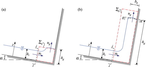
For the sake of simplicity, we consider the velocity distribution on the incoming surge nearly uniform, and consequently we set equal to 1 the momentum and energy correction coefficients.

The control volume contains the whole zone of the flow characterized by a curvature: this entails that at the inflow section all the streamlines are parallel to the bed and at the outflow section all the streamlines are parallel to the vertical wall. With respect to the control volume defined as above, the momentum balance in the longitudinal direction can be written as: $S=\frac{1}{2}{\rho }_{m}g{h}_i^2\cos \alpha +{\rho }_m{u}_i^2{h}_i$ In Eq. (5$S=\frac{1}{2}{\rho }_{m}g{h}_i^2\cos \alpha +{\rho }_m{u}_i^2{h}_i$) $h_i$ and $u_i$ are the depth and velocity of the incoming flow when entering the control volume. In the momentum balance, in first approximation, we neglected the contribution of the longitudinal weight component of the fluid and the bed shear stresses, given that we assumed the length of the base of the control volume to be small enough and that the two forces are opposite. Basically, the impact force is due to the hydrostatic force and the momentum of the incoming flow, since the jet in the outflow section moves in the direction parallel to the wall and it does not contribute to the momentum balance in the direction perpendicular to the wall. Eq. (5$S=\frac{1}{2}{\rho }_{m}g{h}_i^2\cos \alpha +{\rho }_m{u}_i^2{h}_i$) is then made dimensionless with respect to the hydrostatic force of the incoming flow: $\tilde{S}=\frac{\frac{1}{2}(g{\rho }_m{h}_i^2\cos \alpha )+{\rho }_m{u}_i^2{h}_i}{\frac{1}{2}(g{\rho }_m{h_i}^2\cos \alpha )}=1+2\frac{{{\mathsf{F}}_{\mathsf{i}}}^{\mathsf{2}}}{\cos \alpha }$ Thus, we obtain a direct relation between the dimensionless impact force and the Froude number.

2.3. Energy balance for the jet-like behaviour

In order to better understand the development and distribution of the pressures on the wall, it is convenient to apply the energy balance to the control volume shown in Fig. 1b.

In general, the energy balance can be written as: ${\iiint }_{V_c}\frac{\mathrm{\partial }}{\mathrm{\partial }t}\left(\rho e_t\right)\mathrm{d}V+{\oint }_{{\Sigma }_c}\left(\rho e_t\right)\mathit{u}\cdot \mathit{n}\mathrm{d}\Sigma ={\oint }_{{\Sigma }_c}\mathit{F}\cdot \mathit{u}\mathrm{d}\Sigma -\frac{\mathrm{\partial }\mathcal{H}}{\mathrm{\partial }t}$ where $\mathit{F}$ represents the surface forces; $e_t$ the energy of the flow per unit mass; and $\mathrm{\partial }\mathcal{H}/\mathrm{\partial }t$ is the quantity of heat supplied to the control volume by its surroundings per unit time. By assuming a constant temperature of the flow, we comprise in $e_t$ the kinetic energy, $e_k$, and the potential energy, $e_p$, only: $e_t=e_k+e_p=\frac{1}{2}{u}^2+gz\cos \alpha$ The second right-hand term of Eq. (7${\iiint }_{V_c}\frac{\mathrm{\partial }}{\mathrm{\partial }t}\left(\rho e_t\right)\mathrm{d}V+{\oint }_{{\Sigma }_c}\left(\rho e_t\right)\mathit{u}\cdot \mathit{n}\mathrm{d}\Sigma ={\oint }_{{\Sigma }_c}\mathit{F}\cdot \mathit{u}\mathrm{d}\Sigma -\frac{\mathrm{\partial }\mathcal{H}}{\mathrm{\partial }t}$), which represents the energy dissipation, can be neglected because of the reduced dimensions of the control volume.

The first left-hand term of Eq. (7${\iiint }_{V_c}\frac{\mathrm{\partial }}{\mathrm{\partial }t}\left(\rho e_t\right)\mathrm{d}V+{\oint }_{{\Sigma }_c}\left(\rho e_t\right)\mathit{u}\cdot \mathit{n}\mathrm{d}\Sigma ={\oint }_{{\Sigma }_c}\mathit{F}\cdot \mathit{u}\mathrm{d}\Sigma -\frac{\mathrm{\partial }\mathcal{H}}{\mathrm{\partial }t}$) represents the time variation of energy inside the control volume. By assuming that during the formation of the jet the incoming velocity remains constant and that, for the sake of simplicity, the shape of the front of the jet is rectangular with a thickness $b_g$ (as in Fig. 1b), we have: $\begin{array}{rl}{\iiint }_{V_c}\frac{\mathrm{\partial }}{\mathrm{\partial }t}\left(\rho e_t\right)\mathrm{d}V& ={\rho }_m{\left(\frac{1}{2}{u}^2+gz\cos \alpha \right)}_g\frac{\mathrm{\partial }{h}_g}{\mathrm{\partial }t}{b}_g\\ & ={\rho }_m{\left(\frac{1}{2}{u}^2+gz\cos \alpha \right)}_g{u}_g{b}_g\end{array}$ where $u_g$ is the velocity of the front of the jet, and $u_g{b}_g=q$ is the volumetric discharge per unit width. In this case the streamlines at the front of the jet are parallel, so we can assume the binomial $u^2/2+gz\cos \alpha$ to be constant along the thickness $b_g$ of the front, given that the pressure on the front is zero.

The second left-hand term of the energy balance (Eq. 7${\iiint }_{V_c}\frac{\mathrm{\partial }}{\mathrm{\partial }t}\left(\rho e_t\right)\mathrm{d}V+{\oint }_{{\Sigma }_c}\left(\rho e_t\right)\mathit{u}\cdot \mathit{n}\mathrm{d}\Sigma ={\oint }_{{\Sigma }_c}\mathit{F}\cdot \mathit{u}\mathrm{d}\Sigma -\frac{\mathrm{\partial }\mathcal{H}}{\mathrm{\partial }t}$), which represents the flux of the energy across the control surface, is reduced to the flux across the upstream section $h_i$, which is the only portion of control surface crossed by the flow: ${\oint }_{{\Sigma }_c}\left(\rho e_t\right)\mathit{u}\cdot \mathit{n}\mathrm{d}\Sigma ={\int }_{h_i}{\rho }_m\left(\frac{1}{2}{u}^2+gz\cos \alpha \right)(-u\mathrm{d}z)$ The first term on the right-hand side of Eq. (7${\iiint }_{V_c}\frac{\mathrm{\partial }}{\mathrm{\partial }t}\left(\rho e_t\right)\mathrm{d}V+{\oint }_{{\Sigma }_c}\left(\rho e_t\right)\mathit{u}\cdot \mathit{n}\mathrm{d}\Sigma ={\oint }_{{\Sigma }_c}\mathit{F}\cdot \mathit{u}\mathrm{d}\Sigma -\frac{\mathrm{\partial }\mathcal{H}}{\mathrm{\partial }t}$) represents the work of the surface forces. Since the flow velocity at the bed and at the wall is zero, the work of the tangential stresses is zero. This means that we consider only the work of the pressure forces in the upstream section of the control volume, that is ${\int }_{h_i}(-p)(-u)\mathrm{d}z$, so that: ${\oint }_{{\Sigma }_c}\mathit{F}\cdot \mathit{u}\mathrm{d}\Sigma ={\int }_{h_i}-p(-u\mathrm{d}z)={\int }_{h_i}pu\mathrm{d}z$ By combining the energy flux (Eq. 10${\oint }_{{\Sigma }_c}\left(\rho e_t\right)\mathit{u}\cdot \mathit{n}\mathrm{d}\Sigma ={\int }_{h_i}{\rho }_m\left(\frac{1}{2}{u}^2+gz\cos \alpha \right)(-u\mathrm{d}z)$) and the work of the pressure forces (Eq. 11${\oint }_{{\Sigma }_c}\mathit{F}\cdot \mathit{u}\mathrm{d}\Sigma ={\int }_{h_i}-p(-u\mathrm{d}z)={\int }_{h_i}pu\mathrm{d}z$), we obtain: $\begin{array}{rl}& {\int }_{h_i}{\rho }_m\left(\frac{1}{2}{u}^2+gz\right)(-u\mathrm{d}z)-{\int }_{h_i}pu\mathrm{d}z\\ & =-{\left(\frac{1}{2}{u}^2+gz\cos \alpha +\frac{p}{\rho }\right)}_i{\int }_{h_i}u\mathrm{d}z,\end{array}$ provided that, on the right-hand side, the trinomial in brackets is constant along the flow depth $h_i$; this is reasonable having assumed the streamlines to be parallel in this section. Thus, we finally obtain: ${\rho }_{m}q\left[{\left(\frac{1}{2}{u}^2+gz\cos \alpha \right)}_g-{\left(\frac{p}{\rho }+\frac{1}{2}{u}^2+gz\cos \alpha \right)}_i\right]=0$ It is worth noting that Eq. (13${\rho }_{m}q\left[{\left(\frac{1}{2}{u}^2+gz\cos \alpha \right)}_g-{\left(\frac{p}{\rho }+\frac{1}{2}{u}^2+gz\cos \alpha \right)}_i\right]=0$), if divided by ${\rho }_{m}q$, also represents the application of the Bernoulli theorem.

When the jet reaches its maximum height $(h_g{)}_{\mathrm{m}\mathrm{a}\mathrm{x}}$, the velocity $u_g$ of the front of the jet is zero, and the energy balance reduces to: ${\left(z\cos \alpha +\frac{p}{{\rho }_{m}g}+\frac{u^2}{2g}\right)}_i=(h_g{)}_{\mathrm{m}\mathrm{a}\mathrm{x}}\cos \alpha$ Considering that on a streamline on the free surface of the incoming flow $p_i=0$, Eq. (14${\left(z\cos \alpha +\frac{p}{{\rho }_{m}g}+\frac{u^2}{2g}\right)}_i=(h_g{)}_{\mathrm{m}\mathrm{a}\mathrm{x}}\cos \alpha$) becomes: $h_i\cos \alpha +\frac{u_i^2}{2g}=(h_g{)}_{\mathrm{m}\mathrm{a}\mathrm{x}}\cos \alpha$ By making Eq. (15$h_i\cos \alpha +\frac{u_i^2}{2g}=(h_g{)}_{\mathrm{m}\mathrm{a}\mathrm{x}}\cos \alpha$) dimensionless with respect to $h_i$, we obtain: $\frac{(h_g{)}_{\mathrm{m}\mathrm{a}\mathrm{x}}}{h_i}=1+\frac{1}{2\cos \alpha }{\mathsf{F}}_{\mathsf{i}}^{\mathsf{2}}$ This result presumes that the energy dissipation is negligible: this hypothesis seems reasonable because the energy dissipation becomes consistent only after the jet reaches its maximum height and begins to fall on itself; up to this instant Eq. (16$\frac{(h_g{)}_{\mathrm{m}\mathrm{a}\mathrm{x}}}{h_i}=1+\frac{1}{2\cos \alpha }{\mathsf{F}}_{\mathsf{i}}^{\mathsf{2}}$) is reliable.

3. Experimental investigation

The experimental investigation was carried out in the Hydraulics Laboratory of the University of Trento. The experiments were conducted in a tilting channel which is 4 m long and 25 cm wide (Fig. 2a).

Figure 2. Experimental apparatus: (a) diagram of the experimental apparatus, (b) disposition layout of the five pressure transducers on the vertical wall, lengths in centimetres

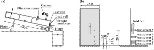
The test wall representing the obstacle was located at the end of the channel, perpendicularly to the bottom. The wall was connected to a load cell, brand HBM (Darmstadt, Germany), measuring the time evolution of the impact force. In order to measure the pressures distribution at different points, five pressure transducers, brand KELLER (Winterthur, Schweiz), were located on the wall (Fig. 2b). The surge was produced by pulling up very rapidly and manually a sluice gate, upstream of which the material (water or mixtures of sand, gravel and water) was stored.

The channel was equipped with an ultrasonic sensor, brand Pepperl+Fuchs (Mannheim, Deutschland) (positioned 1.3 m upstream of the test wall) capable of registering the time evolution of the flow depth (Fig. 2a).

Finally, all the experiments were recorded by two high speed cameras, both Photron FASTCAM-1024PCI (San Diego, CA, UK), with a frame rate of 500 frames per second and a resolution of $1024\times 1024$ pixels. The first was placed laterally, in order to record the evolution of the vertical jet along the test wall and the other was positioned above the channel to record the arrival of the flow front and evaluate its velocity.

The velocity $u_i$, which represents the velocity of the front of the incoming surge, was measured, calculating the time needed for the front to cover the distance (15 cm) between two fixed points located within the channel, at a distance of about 45 and 60 cm from the test wall. In order to identify the position of the two fixed points, we placed two laser pointers normally to the bed. The transit time was obtained from the analysis of the frames recorded by the camera positioned above the channel. In this way it was possible to identify the position of the front with an accuracy of about 1 mm.

The two cameras, the five pressure transducers, the load cell and the ultrasonic sensor were all synchronized during the experiments, through an ad hoc software.

The experimental investigations were done with clear water and a mixture of water and sediments (sand and gravel characterized by $d_{30}=2.0$ mm, $d_{50}=3.5$ mm and $d_{90}=9.0$  mm). The solid fraction concentration ranges between 0.4 and 0.6. Further details on the experimental equipments and on the grain size distribution are given in the Supplemental online material.

4. Results

About 50 tests with clear water and 30 with mixtures of water and sediments were carried out, each with variations in the slope of the channel, the volume released and, in the case of mixtures, the solid fraction. As explained above, we measured the flow depth, the velocity of the flow, the pressures along the vertical wall and the impact force against the wall. A complete list of the test and the experimental values are given in the Supplemental online material (Tables W1 and M).

4.1. Flow depth of the incident surge

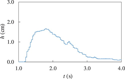
Figure 3 presents an example of the time evolution of the flow depth of the incoming surge recorded by the ultrasonic sensor. The figure shows a continuous variation of the depth in time. We took the maximum flow depth, indicated as $h_i$ in the following, as the geometrical scale for all the dimensionless parameters, and in particular in the definition of the Froude number ${\mathsf{F}}_{\mathsf{i}}\mathsf{=}{\mathsf{u}}_{\mathsf{i}}\mathsf{/}\sqrt{\mathsf{g}{\mathsf{h}}_{\mathsf{i}}}$, where $u_i$ is the velocity of the foot of the front.

Figure 3. Flow depth evolution in time at a fixed position. Clear water: $\mathsf{F}\mathsf{=}\mathsf{4.42}$, Test W1-7

4.2. Impact force

The impact force against the test wall was measured in general by the direct measurement of the force through the load cell. In some tests we measured it also by integrating in each instant the measured pressures (indirect method) (Fig. 4), according to the following hypotheses:

• at each instant the values recorded by the transducers are connected by straight line segments;

• the pressures above the uppermost cell are considered linearly distributed down to zero with the same gradient of the last two cells, given that the jet in the upper part is parallel to the wall and weakly contributes to the impact force;

• the pressure distribution is considered constant across the width of the channel.

Figure 4. Sketch of the integration of the pressures. Mixture of water and sediments: C=0.4, $\mathsf{F}\mathsf{=}\mathsf{4.64}$, Test M-10

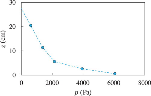
Figure 5a presents the pressures evolution at the five transducers for the clear water test 53.W1, while Fig. 5b presents a comparison of the time evolution of the impact force as measured according to the two methods (by integrating the pressure and by the load cell). In most cases, the indirect and direct measures of the impact force are very similar: this result confirms that the assumptions made for the pressure distribution are reasonable.

Figure 5. Example of a pressure and impact force evolution in time. Clear water: $\mathsf{F}\mathsf{=}\mathsf{7.61}$, Test W1-53; (a) pressures evolution in time at the five pressure transducers located at different heights along the wall, (b) evolution in time of the impact force, as measured directly by the load cell and indirectly by integrating the pressure transducer measurements

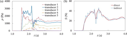
Figure 6 shows the comparison between the maximum impact forces measured trough the load cell and the values obtained theoretically using the momentum balance (Eq. 6$\tilde{S}=\frac{\frac{1}{2}(g{\rho }_m{h}_i^2\cos \alpha )+{\rho }_m{u}_i^2{h}_i}{\frac{1}{2}(g{\rho }_m{h_i}^2\cos \alpha )}=1+2\frac{{{\mathsf{F}}_{\mathsf{i}}}^{\mathsf{2}}}{\cos \alpha }$), solid line) for both clear water and mixtures of water and sediment. In the caption of the figure we reported the value of the relative standard deviation R_SD of the experimental points with respect to the theoretical curve. The R_SD is defined as the ratio of the standard deviation σ of the data to the mean value of the dimensionless force $\tilde{S}$.

Figure 6. Dimensionless maximum impact force as a function of the Froude number for clear water and mixture of water and sediments. Comparison between experimental data and as calculated using momentum balance (Eq. 6$\tilde{S}=\frac{\frac{1}{2}(g{\rho }_m{h}_i^2\cos \alpha )+{\rho }_m{u}_i^2{h}_i}{\frac{1}{2}(g{\rho }_m{h_i}^2\cos \alpha )}=1+2\frac{{{\mathsf{F}}_{\mathsf{i}}}^{\mathsf{2}}}{\cos \alpha }$): (a) clear water, (b) water and sediments for different values of solid concentration

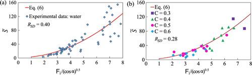
The theoretical curve captures the general trend of the experiments. However, there is a certain dispersion of the data that could have two main causes:

• the non-complete repeatability of the manual opening of the sluice gate of the reservoir upstream in the channel;

• the choice of $h_i$ as the maximum of the flow depth curve: this could cause uncertainties since it is often a single point whose value is affected by the transversal inhomogeneity of the front and by the consequent lack of replicability.

Figure 6a and b highlight a certain difference between the cases of clear water and a mixture of water and sediments: the evolution of the phenomenon in the case of a mixture is slower, so uncertainties related to the manual opening of the sluice gate is reduced. Also, the jet with sediments resulted in being more compact, giving rise to a more defined impact. For these reasons, for the mixture of water and sediments there is less dispersion of the experimental data than in the case of clear water.

4.3. Maximum height of the jet

An important parameter for the design of protection structures against debris flows is the distribution of loads on the vertical wall. For this purpose, we first determined the maximum height of the jet on the test wall.

An initial analysis of the results of the experiments with clear water was carried out by taking the dimensionless measured maximum height of the jet, $(h_g{)}_{\mathrm{m}\mathrm{a}\mathrm{x}}/h_i$, expressed as a function of the Froude number, and comparing it with maximum height predicted using the energy balance (Eq. 16$\frac{(h_g{)}_{\mathrm{m}\mathrm{a}\mathrm{x}}}{h_i}=1+\frac{1}{2\cos \alpha }{\mathsf{F}}_{\mathsf{i}}^{\mathsf{2}}$). In Fig. 7a we observe a good agreement between the experimental data (diamonds) and the prediction of the energy balance (Eq. 16$\frac{(h_g{)}_{\mathrm{m}\mathrm{a}\mathrm{x}}}{h_i}=1+\frac{1}{2\cos \alpha }{\mathsf{F}}_{\mathsf{i}}^{\mathsf{2}}$) (solid line) for clear water. This result confirms that until the jet reaches its maximum height the energy dissipation is negligible.

Figure 7. Dimensionless $(h_g{)}_{\mathrm{m}\mathrm{a}\mathrm{x}}$ versus Froude number for clear water and mixture of water and sediments. Energy balance solution (Eq. 16$\frac{(h_g{)}_{\mathrm{m}\mathrm{a}\mathrm{x}}}{h_i}=1+\frac{1}{2\cos \alpha }{\mathsf{F}}_{\mathsf{i}}^{\mathsf{2}}$) against experimental data: (a) clear water, (b) water and sediments

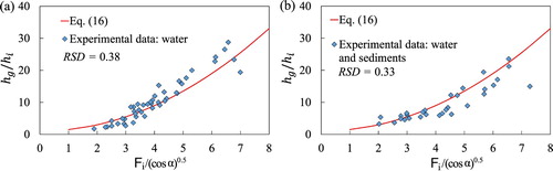
The same analysis was carried out for the mixtures of water and sediment. The results are reported in Fig. 7b. The two figures show a certain dispersion of the data, probably due to the shape of the incoming front and the shape of the front of the jet, which are not rectangular, as we assumed in the application of the energy balance. Besides, in the experiments with mixtures, it is plausible that during the propagation of the jet in the vertical direction a segregation of the solid phase occurs (due to different velocities between the phases).

4.4. Detailed analysis of the pressure distribution and its evolution in time

In some tests the distribution of the pressures along the wall was recorded by the pressure transducers. The records show that the pressure distribution along the wall during the impact cannot be represented by a linear distribution (hydrostatic distribution). This behaviour has been observed for both clear water (Fig. 8) and the mixtures of water and sediments (Fig. 9).

Figure 8. Impact time evolution. Clear water: $\mathsf{F}\mathsf{=}\mathsf{7.04}$, Test W1-50

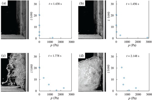
Figure 9. Impact time evolution. Mixture of water and sediment: $\mathsf{F}\mathsf{=}\mathsf{4.64}$, C=0.4, Test M-10

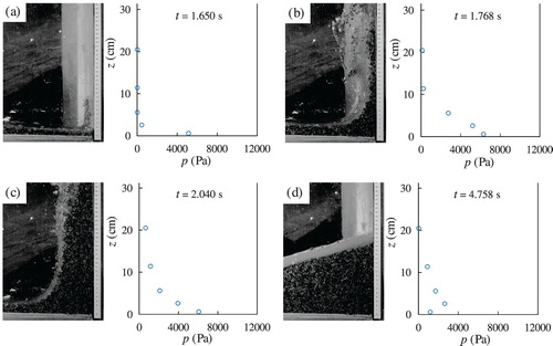
Figure 8 shows some images of the flow impact against the wall, alongside the pressure distribution (on the right). The circles represent the pressure values at different positions as measured by the transducers. In Fig. 8a the flow has just reached the wall; the lowermost transducer starts to register a peak of pressure.

In the next Fig. 8b the flow has clearly assumed a jet-like behaviour. The lowermost cell registers the maximum value of the whole test and the second transducer begins to register a small value of pressure.

In the following Fig. 8c the jet starts to break falling back down upstream of the test wall. The second last transducer registers an over pressure reasonably due to the curvature of the streamlines (as explained below).

In the last Fig. 8d the flow tends to the static condition and the pressure gets close to hydrostatic distribution, but is still strongly disturbed by the free surface fluctuations.

Very similar behaviour can be observed for the mixture of water and sediment in Fig. 9a–d.

In order to explain the pressure behaviour, we refer to the momentum balance in intrinsic coordinates with respect to the normal direction (the second Euler equation) (Fig. 10).

Figure 10. Jet curvature effect: pressure distribution along the vertical wall. Mixture of water and sediment: $\mathsf{F}\mathsf{=}\mathsf{4.64}$, C=0.4, Test M-10: (a) intrinsic coordinates system, (b) flow curvature of the jet

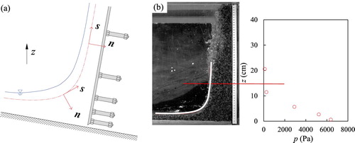
Considering, for the sake of simplicity, the flow as permanent; this equation can be written as follows: $\frac{\mathrm{\partial }}{\mathrm{\partial }n}(p+{\rho }_{m}gz\cos \alpha )=-{\rho }_m\frac{u_s^2}{R}$ where n is the normal intrinsic coordinate, $u_s$ is the longitudinal component of the velocity vector, R is the radius of curvature of the streamline, and z is the direction normal to the bed.

According to Eq. (17$\frac{\mathrm{\partial }}{\mathrm{\partial }n}(p+{\rho }_{m}gz\cos \alpha )=-{\rho }_m\frac{u_s^2}{R}$), when the streamlines are parallel to the wall, R tends to infinity. In this condition, the piezometric head is constant along the coordinate n and, since the relative pressure on the free surface is zero, the pressure on the wall is very small ($p\simeq \rho g{b}_g\sin \alpha$). This is clearly visible in the right-hand diagrams of the sequence of Fig. 8a–d.

Figure 10 shows a frame recorded during an experiment with a water–sediment mixture in which we have highlighted the free surface curvature in the lower part of the jet. Observing the pressure values registered by the pressure transducers, one can notice that in the upper part, where the curvature is zero, the pressure is nearly zero.

The main difference between the impact of clear water and that of a mixture of water and sediments is that the curvature is more pronounced in the clear water (clearly visible in Fig. 8 when compared to Fig. 9). This means that, for clear water, the radius of curvature must tend to infinity more rapidly. An explanation of this different behaviour could be a possible deposit of sediments near the corner. However, the analysis of the recorded images shows that the deposit of sediments process seems to start after the impact has reached its maximum value.

4.5. Transition between reflected wave and jet-like impact

Figure 11 shows an overview of the dimensionless force data of all tests (Table W2 reported in the Supplemental online material). The triangles in the figure represent the experimental data corresponding to a reflected wave, while the circles refer to the jet-like impact. The dashed line represents the solution of the momentum balance under the hypothesis of reflected wave (Eq. 4$\tilde{S}=\frac{S}{\frac{1}{2}{\rho }_{m}g{h}_i^2\cos \alpha }={\left(1+1.51{\left(\frac{{\mathsf{F}}_{\mathsf{i}}}{\sqrt{\cos \alpha }}\right)}^{1.2}\right)}^{5/3}$), while the solid curve represents the solution corresponding to the jet-like configuration (Eq. 6$\tilde{S}=\frac{\frac{1}{2}(g{\rho }_m{h}_i^2\cos \alpha )+{\rho }_m{u}_i^2{h}_i}{\frac{1}{2}(g{\rho }_m{h_i}^2\cos \alpha )}=1+2\frac{{{\mathsf{F}}_{\mathsf{i}}}^{\mathsf{2}}}{\cos \alpha }$).

Figure 11. Clear water: comparison between experimental data and the momentum balance calculated for a reflected wave (Eq. 4$\tilde{S}=\frac{S}{\frac{1}{2}{\rho }_{m}g{h}_i^2\cos \alpha }={\left(1+1.51{\left(\frac{{\mathsf{F}}_{\mathsf{i}}}{\sqrt{\cos \alpha }}\right)}^{1.2}\right)}^{5/3}$) and for a vertical jet scheme (Eq. 6$\tilde{S}=\frac{\frac{1}{2}(g{\rho }_m{h}_i^2\cos \alpha )+{\rho }_m{u}_i^2{h}_i}{\frac{1}{2}(g{\rho }_m{h_i}^2\cos \alpha )}=1+2\frac{{{\mathsf{F}}_{\mathsf{i}}}^{\mathsf{2}}}{\cos \alpha }$)

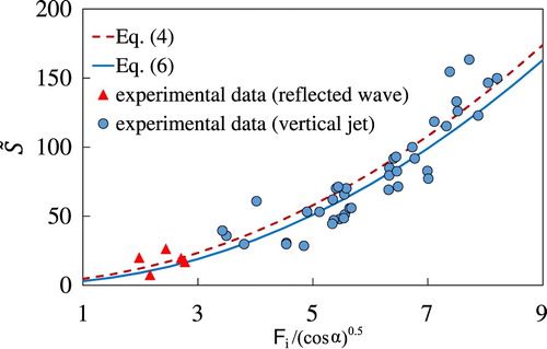
The figure shows that the transition between the two types of impact occurs at ${\mathsf{F}}_{\mathsf{i}}\mathsf{/}\mathsf{(}\cos \alpha {\mathsf{)}}^{\mathsf{0.5}}$ around 3, i.e. Froude numbers greater than $3\sqrt{\cos \alpha }$, or 3 since $\cos \alpha$ is approximately 1. This result is not surprising since the reflected wave is of finite amplitude and it moves with a celerity greater than that of an infinitesimal free surface perturbation.

Notably, Fig. 11 shows how the two theoretical solutions do not differ very much and that the reflected wave solution is always the safer one.

4.6. Impact of single gravel particles

In the analysis presented in the previous sections the mixtures of water, sand and gravel have been treated as homogeneous fluids. There may be doubts that the impact of particles on the obstacle could result in a further pressure not accounted for in the analysis, particularly in the case of larger sediments.

Generally, the pressure exerted by a solid body during a collision with a structure is proportional to the ratio between the impact force and the contact surface, and can be evaluated according to Hertz's equation (Gauer, 2009). When considering the impact of a single gravel particle, this area is often a small part of the particle surface and, therefore, an even smaller portion of the vertical wall. This leads to a big increase of the pressure in that zone, resulting presumably in a peak in the pressure-time evolution of that point. Reasonably, the collision of the particle is not perfectly elastic, so that its deformation and that of the vertical wall absorb part of the force during the impact. The energy is dissipated as heat or vibration of the structure. The presence of water and the smaller sediments increases the dissipation by damping the impact.

Furthermore, the distribution of the stresses is characterized by a strong compression at the impact surface and bending stresses a short distance away.

In our experiments, one might expect that the impact of the bigger gravels on a cell would induce a strong peak of pressure on it.

To highlight this aspect, in some tests we inserted four pressure cells in four points located on the test wall at the same height (z=5.8 cm) from the bottom and distant 5 cm one from the other. Interestingly, we observed that in the early stage of the impact (e.g. in the first 0.5 s after the impact) one single transducer measured a pressure peaks even 3–5 times higher than that pressure recorded in the same instant by the other three transducers. Figure 12 shows this behaviour for the test 25M, but the same occurrence was observed also in other tests with sediment mixtures.

Figure 12. Example of the transversal pressures distribution. Mixture of water and sediment: $\mathsf{F}\mathsf{=}\mathsf{3.36}$, C=0.5, Test M-25

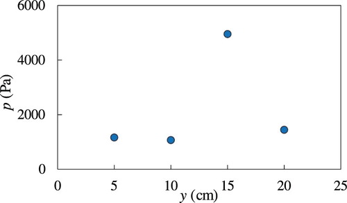
This suggests that the pressure peak is due to the impact of a single gravel particle on the pressure transducer.

The influence of the presence of gravel has been analysed by the time evolution of the fluctuating component of pressure, $\delta p$, with respect to a moving average of the pressure, calculated with five consecutive values, for both clear water (Fig. 13a) and a mixture of water and sediments (Fig. 13b). A comparison of the two figures shows that, in the presence of gravel, the intensity of the fluctuating pressure is much more pronounced than for clear water.

Figure 13. Example of the evolution in time of the fluctuating component of pressure on the wall, measured at the transducers 1 and 2 respectively: (a) clear water: $\mathsf{F}\mathsf{=}\mathsf{3.4}$, Test W2-30, (b) mixture of water and sediments: $\mathsf{F}\mathsf{=}\mathsf{3.36}$, C=0.5, Test M-25

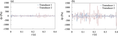
This analysis is in agreement with Lei, Cui, Zeng, and Guo (2017), which analysed in depth the signal recorded during the impact of a mixture of water and sediments.

However, since the peaks described above are local, it is reasonable to assume that they do not significantly affect the total impact force. For this reason, in order to calculate the impact force from the pressure (indirect method described in the previous chapter) the peaks were damped.

From a design point of view, the force exerted by a single boulder little affect the total impact force. However, it should be taken into account in order to prevent local damage effects on the structure.

4.7. Considerations on similarity

From Eqs (4$\tilde{S}=\frac{S}{\frac{1}{2}{\rho }_{m}g{h}_i^2\cos \alpha }={\left(1+1.51{\left(\frac{{\mathsf{F}}_{\mathsf{i}}}{\sqrt{\cos \alpha }}\right)}^{1.2}\right)}^{5/3}$) and (6$\tilde{S}=\frac{\frac{1}{2}(g{\rho }_m{h}_i^2\cos \alpha )+{\rho }_m{u}_i^2{h}_i}{\frac{1}{2}(g{\rho }_m{h_i}^2\cos \alpha )}=1+2\frac{{{\mathsf{F}}_{\mathsf{i}}}^{\mathsf{2}}}{\cos \alpha }$) we deduce that the impact force depends only on the geometry and the Froude number of the front. This means that the results obtained can be transferred to real scale according to these two similarity criteria. However in reality, the parameters affecting debris flow mechanics are many more (Iverson, 2015). Generally, we can treat debris flows as two-phase fluids composed of water and well-mixed solid particles, which constitute the granular phase. In this case, in addition to the elementary internal forces of the interstitial fluid, one must consider the interactions between the particles (internal forces of the granular phase) and the forces of interaction between the two phases.

However, according to Armanini (2015), uniform flows of this type are basically dependent only on the Froude number of the mixture, the solid phase concentration, and the ratio of the $d_{50}$ of the granular phase to the flow depth. In the absence of cohesive material in the solid phase, the influence of interstitial fluid viscosity is completely negligible.

Notice, however, that the above considerations mainly concern the conditions upstream of the impact, which in the case of real debris flows should be provided by appropriate mathematical models. In deriving Eqs (4$\tilde{S}=\frac{S}{\frac{1}{2}{\rho }_{m}g{h}_i^2\cos \alpha }={\left(1+1.51{\left(\frac{{\mathsf{F}}_{\mathsf{i}}}{\sqrt{\cos \alpha }}\right)}^{1.2}\right)}^{5/3}$) and (6$\tilde{S}=\frac{\frac{1}{2}(g{\rho }_m{h}_i^2\cos \alpha )+{\rho }_m{u}_i^2{h}_i}{\frac{1}{2}(g{\rho }_m{h_i}^2\cos \alpha )}=1+2\frac{{{\mathsf{F}}_{\mathsf{i}}}^{\mathsf{2}}}{\cos \alpha }$), we have in fact adopted the perfect fluid hypothesis, which is that the Froude number and the geometry are the only parameters responsible for the impact force if it is expressed in function of the kinematics of the flow upstream of the obstacle just before impact.

In this work, we have not considered debris flows with high percentages of clay. However, when the Froude number is high enough, the inertial forces are much greater then the viscous forces and cohesion forces. In this case, we expect the role of cohesion to be negligible. Nevertheless, the study of the impact in the presence of cohesive material at low Froude numbers deserves an in-depth ad hoc experimental analysis.

5. Conclusions

In the present work we address the problem of the dynamic impact of gravitational granular flows, which is essential in the definition of proper design criteria for protective structures in mountain areas.

From the literature we know that the impact of a surge of a debris flow on a vertical wall can occur in two different ways: as a reflected wave or as a jet. In our experiments we found that the type of impact that occurs depends on the Froude number of the incoming front; for ${\mathsf{F}}_{\mathsf{i}}\mathsf{<}\sim \mathsf{3}$, a reflected wave forms, otherwise it is a vertical jet. Such high values of the Froude number for the transition between the two types of impact are due to the finite amplitude of the reflected wave. Since the solution of the reflected wave was already known, we focused our attention on the vertical jet case.

By applying the momentum balance to the control volume defined in Fig. 1, in which the flow at the entry section is perpendicular to the test wall and the flux at the outgoing section is parallel to it, we obtained a simplified formulation to evaluate the impact force against an obstacle. It consists of the hydrostatic force and the momentum entering the control volume, since they are the only components perpendicular to the wall. This shows that the approximation often used in the past, which considers the impact force to be proportional to the hydrostatic force, is not realistic and that the hydrodynamic contribution is fundamental. Hence, if the force is made dimensionless with respect to the hydrostatic force of the incoming surge, the impact is, in good approximation, independent from the rheological and constitutive relations of the material composing the debris flow.

It must be noted that we assumed a rectangular surge, but an oblong and irregular front could cause a variation of the impact force with respect to the above equations. Our experimental data show a relative standard deviation of the dimensionless impact force around 0.3–0.4. Therefore, in the applications it is necessary to take into account this uncertainty, together with the uncertainties related to other parameters.

By applying the energy balance to a control volume containing the whole jet, we found that the maximum height of the jet can be easily computed with a simplified energy balance. Comparison with the experimental results confirms that the approximations adopted to derive the simplified solution are acceptable.

Furthermore, we analysed the pressures distribution of the jet along the test wall by using five pressure transducers. We found that the pressure distribution along the wall is strongly nonlinear, that is to say, it is not hydrostatic. In particular, we explained this behaviour with the second Euler equation: the evolution of the pressure is related to the curvature radius of the flow at different heights in a non linear form. Notably, at a certain height when the curvature is practically zero, the pressure along the wall becomes negligible.

Through our experimental investigation, we compared the simplified formulations described above with the experimental results, always finding good agreement.

Finally, we also evaluated the effect of the impact of gravel particles on the wall. By comparing the impact of a surge of clear water with that of a mixture of water and sediments, we observed that in the latter case the pressure fluctuations are larger due to the impacts of gravel particles. However, this is a local effect and, reasonably, it has little influence on the global impact force on the obstacle.

Notation

a	=	celerity of the reflected wave (m s−1)
$b_g$	=	surface forces (m)
C	=	solid concentration (–)
$e_k$	=	kinetic energy per unit mass (m−2 s−2)
$e_p$	=	potential energy per unit mass (m−2 s−2)
$e_t$	=	flow energy per unit mass (m−2 s−2)
$\mathit{f}$	=	mass forces (kg m s−2)
$\mathit{F}$	=	surface forces (kg m s−2)
F	=	Froude number (–)
g	=	gravity acceleration (m s−2)
$h_g$	=	height of the jet (m)
$h_i$	=	flow depth of the incident flow (m)
$h_r$	=	flow depth of the reflected wave (m)
$\mathcal{H}$	=	quantity of heat supplied to control volume (kg m2 s−3)
n	=	normal intrinsic coordinate (m)
$\mathit{n}$	=	vector normal to the surface (m)
p	=	pressure (kg m−1 s−2)
q	=	volumetric discharge per unit width (m2 s−1)
R	=	radius of the jet curvature (m)
s	=	tangential intrinsic coordinate (m)
S	=	impact force (kg m s−2)
$\mathit{u}$	=	velocity vector (m s−1)
$u_i$	=	incident flow velocity (m s−1)
$u_r$	=	reflected wave velocity (m s−1)
$u_s$	=	velocity component along the intrinsic coordinate $s$ (m s−1)
${\rho }_m$	=	density of the mixture (kg m−3)

Acknowledgments

The authors express their special thanks to Professor Casulli for helpful discussions and suggestions. The authors are grateful to Andrea Rodler and Federico Ress, who made a great contribution to the work during their Master Thesis period. Finally, the authors would thank the technicians of the Hydraulic Laboratory of the University of Trento, who always supported the experimental work.

Supplemental data

Supplemental data for this article can be accessed http://dx.doi.org/10.1080/00221686.2019.1579113

Additional information

Funding

The Research is part of the project PRIN 2015 of MIUR.

References

- Arattano, M., Deganutti, A. M., & Marchi, L. (1997). Debris flow monitoring activities in an instrumented watershed on the Italian alps. In C. Chen (Ed.), Debris-flow hazards mitigation: Mechanics, prediction, and assessment (pp. 506–515). New York: ASCE.
- Armanini, A. (2009). Discussion on: Experimental analysis of the impact of dry avalanches on structures and implication for debris flow (Zanuttigh, Lamberti). Journal of Hydraulic Research, 47(3), 381–383. doi: 10.1080/00221686.2009.9522009
- Armanini, A. (2015). Closure relations for mobile bed debris flows in a wide range of slopes and concentrations. Advances in Water Resources, 81, 75–83. doi: 10.1016/j.advwatres.2014.11.003
- Armanini, A., Larcher, M., & Odorizzi, M. (2011). Dynamic impact of a debris flow front against a vertical wall. In Proceedings of the 5th international conference on debris-flow hazards mitigation: Mechanics, prediction and assessment (pp. 1041–1049). Padua, Italy.
- Armanini, A., & Scotton, P. (1992). Experimental analysis on the dynamic impact of a debris flow on structures. In Proceedings of the international symposium interpreavent (pp. 107–116), Bern.
- Aulitzky, H. (1990). Vorläufige studienblätter zu der vorlesung wildbach-u. lawinenverbauung. Universität für Bodenkultur.
- Cui, P., Zeng, C., & Lei, Y. (2015). Experimental analysis on the impact force of viscous debris flow. Earth Surface Processes and Landforms, 40(12), 1644–1655. doi: 10.1002/esp.3744
- Davies, T. R. H. (1985). The investigation of avalanche processes by laboratory experiments; exploratory tests. Proceedings of the international symposium on erosion, debris flow and disaster prevention (pp. 215–218), Tsukuba, Japan.
- Daido, A. (1993). Impact force of mud-debris flows on structures. In proceedings of the congress-international association for hydraulic research (Vol. 3, pp. 211–211). Local Organizing Committee of the xxv Congress.
- Gauer, P. (2009). Loads due to impact of solid bodies. In T. Jóhannesson, P. Gauer, P. Issler, K. Lied, K. M. Hákonardóttir, et al. (Eds.), The design of avalanche protection dams: Recent practical and theoretical developments (pp. 109–112). Brussels: European Commission.
- Ghilardi, P., Pagliardi, M., & Zanuttigh, B. (2006). Experimental analysis of the impact process of granular saturated mixtures against vertical walls. In XXX Convegno Nazionale di Idraulica e Costruzioni Idrauliche.
- Henderson, F. M. (1966). Open channel flow. New York, NY: McMillan Pubblishing.
- Huang, H.-P., Yang, K.-C., & Lai, S.-W. (2007). Impact force of debris flow on filter dam. Geophys Res. Abstr. Eur. Geosci., 9, 03218.
- Iverson, R. M. (1997). The physics of debris flows. Reviews of Geophysics, 35(3), 245–296. doi: 10.1029/97RG00426
- Iverson, R. M. (2015). Scaling and design of landslide and debris-flow experiments. Geomorphology, 244, 9–20. doi: 10.1016/j.geomorph.2015.02.033
- Jakob, M., Hungr, O., & Jakob, D. M. (2005). Debris-flow hazards and related phenomena (Vol. 739). Berlin: Springer.
- Lei, Y., Cui, P., Zeng, C., & Guo, Y. (2017). An empirical mode decomposition-based signal process method for two-phase debris flow impact. Landslides, 15, 1–11.
- Lichtenhahn, C. (1973). Berechnung von sperren in beton und eisenbeton. Mitt Forstl Bundes versuchsanst Wein.
- Mizuyama, T., Ishikawa, Y., & Ishikawa, Y. (1988). Technical standard for the measures against debris flow (draft). Sabo (Erosion Control) Division, Sabo Department, Public Works Research Institute, Ministry of Construction.
- Moriguchi, S., Borja, R. I., Yashima, A., & Sawada, K. (2009). Estimating the impact force generated by granular flow on a rigid obstruction. Acta Geotechnica, 4(1), 57–71. doi: 10.1007/s11440-009-0084-5
- Takahashi, T. (1980). Debris flow on prismatic open channel. Journal of the Hydraulics Division, 106(3), 381–396.
- Vagnon, F., & Segalini, A. (2016). Debris flow impact estimation on a rigid barrier. Natural Hazards and Earth System Sciences, 16(7), 1691–1697. doi: 10.5194/nhess-16-1691-2016
- Watanabe, M., & Ikeya, H. (1981). Investigation and analysis of volcanic mud flows on Mount Sakurajima Japan. Erosion sediment transport measurement. International Association on Hydrology, 133, 245–256.
- Zanuttigh, B., & Lamberti, A. (2007). Instability and surge development in debris flows. Reviews of Geophysics, 45(3). doi: 10.1029/2005RG000175