Prediction of flow around a sharp-nosed bridge pier: influence of the Froude number and free-surface variation on the flow field

Abstract

This study investigates the influence of free-surface variation on the velocity field using numerical simulations of flow around a sharp-nosed pier that is representative of a typical masonry bridge pier. The study evaluates the assumption that free-surface effects are negligible at small Froude numbers by comparing the change in flow field predictions due to the use of a free-surface model (i.e. multi-phase simulation with a volume of fluid (VOF) model in place of a rigid-lid approximation (i.e. single phase simulation). Results show that simulations using the VOF model are in better agreement with experimental data than those using the rigid-lid approximation. Importantly, results show that even though the change in free-surface height near the pier is small comparative to the approach flow, it still has a significant effect on velocities in front of the pier and in the wake region, and including at low Froude numbers.

Keywords:

• Computational fluid dynamics
• Froude number
• OpenFOAM
• pier
• volume of fluid

1. Introduction

The flow around hydraulic structures such as bridge piers is very complex due to the constant shearing of the approaching flow generating multiple vortex systems (e.g. horseshoe, lee-wake systems) and complicated free-surface interactions. These processes are largely responsible for the initiation and development of scour (Breusers, Nicollet, & Shen, 1977), a phenomenon that can have a significant deleterious effect on the structural integrity of bridges, particularly during flood events. Masonry bridge piers are particularly at high risk of scour due to their large width-to-length ratio and their unique geometries, which often includes triangle cut-waters (i.e. sharp noses). These structures make up nearly 40% of the UK's current bridge stock with a significant number listed as cultural and engineering heritage structures. They also pose a bigger obstruction to flow due to their much larger width-to-length ratio that is needed to support the weight of the bridge. Consequently, understanding the flow around masonry bridge piers and their impact on scour is of critical importance in the context of flood resilience of transport networks.

Numerous authors have investigated the computational modelling of fluid flow and scour around bridge piers (Baranya, Olsen, Stoesser, & Sturm, 2012, 2014; Huang, Yang, & Xiao, 2009; Richardson & Zaki, 1997; Roulund, Sumer, Fredsoe, & Michelson, 2005). The majority of these investigations focus on circular piers due to their strong ties to the classical fluid dynamics problem of flow around cylinders. The flow around sharp nosed bridge piers, common in masonry bridges, has received little attention in the literature despite its clear engineering relevance. To the authors' knowledge, the geometry closest to the sharp nosed pier in the literature is the diamond shaped pier employed by Khosronejad, Kang, and Sotiropoulos (2012). The current study seeks to address this gap by investigating a typical sharp nosed bridge pier.

The numerical simulation of flow around bridge piers requires selection of an approach to model free-surface flow. There are currently two common ways of modelling free-surface flow: (1) through a rigid-lid approximation that essentially models an artificial rigid free surface along which the tangential velocities can be non-zero; or (2) through a free-surface tracking approach in which both the water and air phases are modelled explicitly. Because of its relative simplicity and lower computational cost, the rigid-lid approximation has been widely used. For example, a notable and relevant study that followed this approach is the one by Richardson and Panchang (1998) who conducted simulations using various bed profiles representative of a flat bed, an intermediate scour hole and an equilibrium scour hole. The primary source of evidence in support of using the rigid-lid approximation for low Froude numbers was given by Graf and Yulistiyanto (1998). Graf and Yulistiyanto (1998) conducted two physical experiments on a circular pier for Froude numbers of 0.5 and 0.2 respectively, and showed that for the lower values of Froude number there was negligible influence on the free-surface profile around the pier. This finding was also confirmed in the study by Roulund et al. (2005), whose model validated well with experimental data for a Froude number of 0.14.

For free-surface tracking, the volume of fluid (VOF) or the level-set method (LSM) is often employed. Both these methods involve significantly more computational cost than the rigid-lid approximation. The VOF method smears the interface between the two phases using a volume fraction function, which is also solved as part of the solution process for the numerical simulation. The LSM, on the other hand, employs a distance function to define explicitly the interface between the two phases. There are several notable studies (Burkow & Griebel, 2016; Chu, Chung, Wu, & Wang, 2016; Kang & Sotiropoulos, 2015; Kara, Kara, Stoesser, & Sturm, 2015; Sajedeh, Farsadizadeh, Arvanagh, & Abbaspour, 2016) using these approaches for hydraulic structures. Of direct relevance to this study is the work by Kara et al. (2015). They compared free surface simulations using LSM with simulations using a rigid-lid approximation for flow around a bridge abutment at a Froude number of 0.43. This value of the Froude number is significantly higher than the previously mentioned limit of 0.2 but represents a very common range of Froude number for laboratory scale experiments. When comparing predictions from the two kinds of simulations, Kara et al. (2015) not only found considerable differences in the flow field but commented that, due to the complex free-surface interaction around the structure, the predicted turbulence behaviours were also markedly different. However, a key drawback of this study is that the mean flow turbulence statistics were not compared against those from experiments. Also, this still leaves the question of whether rigid-lid approximations are sufficient for flows with Froude numbers less than 0.2 unanswered.

Assessing the reliability of a rigid-lid approximation is essential for building confidence in predictions based on simulations using this approximation. For example, in the study by Richardson and Panchang (1998) cited above, the depth of the scour hole may have potentially been overestimated due to the use of a rigid-lid approximation, but the extent of overestimation is unknown due to the lack of comparison with results from a numerical model including the free surface. Our study addresses this important drawback. The objectives of this paper are thus as follows:

1. to investigate and quantify the fluid flow behaviour in the vicinity of a typical masonry bridge (sharp-nosed) pier;

2. to ascertain using a free-surface model, the effect of the free-surface variation on flow characteristics around this type of pier; and

3. to provide guidance on the Froude number range for which a rigid-lid approximation is likely to provide reliable results.

In order to achieve these objectives, a sharp-nosed pier that is representative of masonry bridge piers is selected for investigation using a rigid-lid approximation and a VOF model. The open-source computational fluid dynamics (CFD) toolbox OpenFOAM is employed to simulate the flow behaviour and model the free surface variation. Numerical results are validated against experimental data collected from a flume experiment conducted at the University of Exeter. The influence of the free-surface variation on velocity field is ascertained using simulations for a range of Froude number values.

2. Numerical model

The Reynolds averaged Navier–Stokes (RANS) equations for an isothermal, incompressible, immiscible fluid are solved for numerically simulating the flow around bridge piers. The equations need to be solved together with a suitable turbulence model for at least the water phase and an appropriate model to represent the free surface. These features are outlined briefly below.

2.1. Governing equations

The RANS equations for mass and momentum conservation are as follows: (1) $\begin{array}{rl}& \mathrm{\nabla }\cdot \mathit{U}=0\end{array}$(1) (2) $\begin{array}{rl}& \frac{\mathrm{\partial }\left(\rho \mathit{U}\right)}{\mathrm{\partial }t}+\mathrm{\nabla }\cdot \left(\rho \mathit{U}\mathit{U}\right)-\mathrm{\nabla }\cdot \left(\right(\mu +{\mu }_t\left)\mathbf{\text{{S}}}\right)=-\mathrm{\nabla }p+\rho \mathit{g}+\mathit{F}\end{array}$(2) In the above equations, $\mathit{U}$ is the velocity vector field, p is the pressure field, μ is the laminar viscosity, ${\mu }_t$ is the turbulent viscosity given by the turbulence model, $\mathbf{\text{{S}}}$ is the strain rate tensor defined as $\mathbf{\text{{S}}}=1/2(\mathrm{\nabla }\mathit{U}+\mathrm{\nabla }{\mathit{U}}^{\mathit{T}})$, $\mathit{F}$ represents the volumetric surface tension force and $\rho \mathit{g}$ represents the gravitational body force.

This paper compares results from single- and multi-phase simulations. The single-phase simulations use a rigid-lid approximation, where the free surface is represented by a domain boundary, i.e. a horizontal plane at a predetermined depth with a slip velocity condition. This assumption leads to both $\mathit{F}$ and $\rho \mathit{g}$ in Eq. (2(2) $\begin{array}{rl}& \frac{\mathrm{\partial }\left(\rho \mathit{U}\right)}{\mathrm{\partial }t}+\mathrm{\nabla }\cdot \left(\rho \mathit{U}\mathit{U}\right)-\mathrm{\nabla }\cdot \left(\right(\mu +{\mu }_t\left)\mathbf{\text{{S}}}\right)=-\mathrm{\nabla }p+\rho \mathit{g}+\mathit{F}\end{array}$(2) ) being zero. In the multi-phase simulations, the air–water interface is calculated using a numerical model rather than being fixed a priori. Multi-phase simulations in this study employ the VOF model which is briefly outlined next.

2.2. Volume of fluid (VOF)

The VOF model is chosen due to its inherent ability to conserve mass in each individual phase. Equations (1(1) $\begin{array}{rl}& \mathrm{\nabla }\cdot \mathit{U}=0\end{array}$(1) ) and (2(2) $\begin{array}{rl}& \frac{\mathrm{\partial }\left(\rho \mathit{U}\right)}{\mathrm{\partial }t}+\mathrm{\nabla }\cdot \left(\rho \mathit{U}\mathit{U}\right)-\mathrm{\nabla }\cdot \left(\right(\mu +{\mu }_t\left)\mathbf{\text{{S}}}\right)=-\mathrm{\nabla }p+\rho \mathit{g}+\mathit{F}\end{array}$(2) ) are solved for the velocity and pressure fields in both water and air phases together with a volume fraction function α that represents the volume of each phase in each cell. α can take any value between 0 and 1. $\alpha =0$ corresponds to the cell being fully occupied by air and $\alpha =1$ corresponds to the cell being fully occupied by water. An advection equation for α can be written as follows: (3) $\frac{\mathrm{\partial }\alpha }{\mathrm{\partial }t}+\mathrm{\nabla }\cdot \left(\alpha \mathit{U}\right)=0$(3) The volume fraction function smears the air–water interface over the cell volumes. To reduce the smearing, the counter-gradient transport algebraic equation is employed. The method adds the compressive velocity term ${\mathit{U}}_{\mathit{c}}$ into Eq. (3(3) $\frac{\mathrm{\partial }\alpha }{\mathrm{\partial }t}+\mathrm{\nabla }\cdot \left(\alpha \mathit{U}\right)=0$(3) ) and also results in better conservation, convergence and boundedness (Weller, Tabor, Jasak, & Fureby, 1998). Thus, Eq. (3(3) $\frac{\mathrm{\partial }\alpha }{\mathrm{\partial }t}+\mathrm{\nabla }\cdot \left(\alpha \mathit{U}\right)=0$(3) ) becomes: (4) $\frac{\mathrm{\partial }\alpha }{\mathrm{\partial }t}+\mathrm{\nabla }\cdot \left(\mathit{U}\alpha \right)+\mathrm{\nabla }\cdot \left({\mathit{U}}_{\mathit{c}}\alpha \beta \right)=0$(4) where (5) $\begin{array}{rl}{\mathit{U}}_{\mathit{c}}& ={\mathit{U}}_2-{\mathit{U}}_1\end{array}$(5) (6) $\begin{array}{rl}\beta & =1-\alpha \end{array}$(6) In the above equations, ${\mathit{U}}_1$ and ${\mathit{U}}_2$ are the velocities of the two phases – water and air respectively. In order to limit dispersion at the interface, the compressive velocity ${\mathit{U}}_{\mathit{c}}$ is only calculated with its components normal to the interface and reads: (7) ${\mathit{U}}_{\mathit{c}}=min(c_{\alpha }|\mathit{U}|,max(|\mathit{U}|\left)\right)\frac{\mathrm{\nabla }\alpha }{|\mathrm{\nabla }\alpha |}$(7) where $c_{\alpha }$ is the compression coefficient. Equation (4(4) $\frac{\mathrm{\partial }\alpha }{\mathrm{\partial }t}+\mathrm{\nabla }\cdot \left(\mathit{U}\alpha \right)+\mathrm{\nabla }\cdot \left({\mathit{U}}_{\mathit{c}}\alpha \beta \right)=0$(4) ) needs special treatment to ensure the conservation law for the phase volume fraction is satisfied while also keeping α bounded between 0 and 1. Therefore, the so-called multidimensional universal limiter with explicit solution (MULES) method is used within a flux-corrected transport algorithm (Zalesak, 1979) in this study.

The density ρ and viscosity μ in the domain are given by: (8) $\begin{array}{rl}\rho & =\alpha {\rho }_1+(1-\alpha ){\rho }_2\end{array}$(8) (9) $\begin{array}{rl}\mu & =\alpha {\mu }_1+(1-\alpha ){\mu }_2\end{array}$(9) where ${\rho }_i$ and ${\mu }_i$ are the density and viscosity of phase i with i=1 representing water and i=2 representing air. The volumetric surface tension force $\mathit{F}$ (Eq. (2(2) $\begin{array}{rl}& \frac{\mathrm{\partial }\left(\rho \mathit{U}\right)}{\mathrm{\partial }t}+\mathrm{\nabla }\cdot \left(\rho \mathit{U}\mathit{U}\right)-\mathrm{\nabla }\cdot \left(\right(\mu +{\mu }_t\left)\mathbf{\text{{S}}}\right)=-\mathrm{\nabla }p+\rho \mathit{g}+\mathit{F}\end{array}$(2) )) in VOF is calculated using the continuum surface force (CSF) model proposed by Brackbill, Kothe, and Zemach (1992): (10) $\mathit{F}=\sigma \kappa \mathrm{\nabla }\alpha$(10) where σ is the surface tension and κ is the free-surface curvature based on the updated value of α after advection. κ is the mean curvature of the free surface and is determined as: (11) $\kappa =-\mathrm{\nabla }\cdot {\mathit{n}}_{\mathit{c}}$(11) where ${\mathit{n}}_{\mathit{c}}$ is the unit normal vector and is calculated as: (12) ${\mathit{n}}_{\mathit{c}}=\frac{(\mathrm{\nabla }\alpha {)}_f}{|(\mathrm{\nabla }\alpha {)}_f|}$(12) where $(\mathrm{\nabla }\alpha {)}_f$ is the cell face value.

2.3. Turbulence model

The k-ω shear stress transport (SST) model (Menter, 1994) is chosen to model turbulence in this study. This model has been shown to offer superior performance compared to other turbulence models for simulation of flows with adverse pressure gradients (Menter, 1994). Moreover Roulund et al. (2005), who employed this model for simulating the turbulent fluid flow around a bridge pier, showed that it can resolve clearly the horseshoe vortex and the lee wake processes and also match the pressure distribution on the face of the pier. More recently, Khosronejad et al. (2012) also reported that unsteady Reynolds-averaged Navier–Stokes (URANS) simulation with k-ω SST model is capable of resolving the basic fluid flow behaviour around a diamond shaped pier, which is close to the pier geometry considered in this study.

For reasons of brevity, only a brief overview of the k-ω SST model is presented here. Readers are referred to Menter (1994) for a detailed description of the model. The turbulent kinetic energy transport equation for the k-ω SST model is as follows: (13) $\frac{\mathrm{\partial }\left(\rho k\right)}{\mathrm{\partial }t}+\mathrm{\nabla }\cdot \left(\rho \mathit{U}k\right)=\mathbf{\text{{P}}}-{\beta }^{\ast }\rho k\omega +\mathrm{\nabla }\cdot \left[\left(\mu +\frac{{\mu }_t}{{\sigma }_k}\right)\mathrm{\nabla }k\right]$(13) The right hand side (RHS) terms represent production, dissipation and diffusion of the turbulent kinetic energy k. The turbulent kinetic energy dissipation transport equation is as follows: (14) $\begin{array}{rl}& \frac{\mathrm{\partial }\left(\rho \omega \right)}{\mathrm{\partial }t}+\mathrm{\nabla }\cdot \left(\rho \mathit{U}\omega \right)={\gamma }_1\rho {\mathbf{\text{{S}}}}^2-\beta \rho {\omega }^2+\mathrm{\nabla }\cdot \left[\left(\mu +\frac{{\mu }_t}{{\sigma }_{\omega }}\right)\mathrm{\nabla }\omega \right]\\ & +2(1-F_1)\rho {\sigma }_{{\omega }_2}\frac{1}{\omega }\mathrm{\nabla }k\mathrm{\nabla }\omega \end{array}$(14) The first three RHS terms represent production, dissipation and diffusion of the specific dissipation ω with the final term representing the blending term used for near wall treatment.

2.4. Computational set-up and operating conditions

The computational model is based on the set-up used in flume experiments by Ebrahimi et al. (2017, 2018). The geometry of the computational model, given in Fig. 1, essentially replicates the flume containing the pier. The boundary conditions of the computational model are highlighted in Fig. 1 and defined in Table 1. The dimensions of the symmetric pier model are given in Fig. 1.

Figure 1. Schematic of flow domain with boundary conditions $5.0\mathrm{m}\times 0.4\mathrm{m}\times 0.6\mathrm{m}$

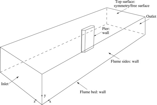
Table 1. Boundary conditions.

Parameter	Inlet	Outlet	Wall	Top
$\mathit{U}$	0.43 (m s^−1)	zeroGradient	zeroGradient	zeroGradient
p	fixedFluxPressure	fixedFluxPressure	fixedFluxPressure	atmosphere
k	0.003 (m^2 s^−2)	zeroGradient	wall function	zeroGradient
ω	0.3 (s^−1)	zeroGradient	wall function	zeroGradient

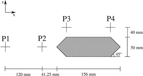
Measurements from flume experiments performed for a specific flow scenario as outlined in Table 2 are used for validation of the computational model. In the experiment, velocity profiles across the depth were measured at four locations around the pier, as shown in Fig. 2, using an acoustic Doppler velocimeter (Vectrino Profiler ADV, Nortek Group, Rud, Norway). Additionally, velocities at four spanwise sections downstream of the pier were also measured to investigate the wake region. These sections were at distances 0.255w, 0.338w, 0.4w and 0.455w from the centre of the pier, where w is the width of the flume. The measurements were taken at a flow depth corresponding to $y/d=1.5$, where y is distance from flume bed and d is pier width.

Table 2. Operating conditions.

Experiment	Flow depth y (m)	Discharge Q (m^3 s^−1)	Reynolds number (R)	Froude number (F)
Pier	0.133	0.035	58,349	0.421

Figure 2. Location of the velocity sampling points

Solving any formulation of the Navier–Stokes equations numerically is challenging because of the tight coupling between the dependent variables and the inherent nonlinearity of the equations. Typically this is accomplished by a sequential solution process in which the governing equations are discretized into a system of linear algebraic equations. The transient equations are solved using the pressure implicit with splitting of operator (PISO) (Issa, 1986) algorithm, which is an extension of the semi-implicit method for pressure linked equations (SIMPLE) family (Ferziger & Peric, 1996; Versteeg & Malalasekera, 1995) that is used for steady-state calculations. This work employs an approach that combines the two algorithms – PISO and SIMPLE. The approach is referred to as the PIMPLE algorithm (Moukalled, Mangani, & Darwish, 2015) – this enables under-relaxation and a momentum predictor to be solved enhancing convergence and robustness. This study uses the implementations of PIMPLE within the open-source toolbox OpenFOAM (Weller et al., 1998) and has been shown to provide good performance in multiphase simulations (Riella, Kahraman, & Tabor, 2018, 2019). Finally, time derivatives are discretized using the Crank–Nicholson scheme and all spatial discretizations are of second order using least squares (gradient), linear upwind (divergence) and central difference (Laplacian).

Simulations are run at the Isca high performance computing facility at the University of Exeter using 16 Intel Haswell E5-2640v3 2.6 GHz CPUs (Santa Clara, California, United States). The influence of mesh size and sampling time on the solution is assessed using simulations run for increasing values for these two parameters. Sampling time is defined as the time over which results are sampled after the simulation has reached convergence. The simulation is found to attain convergence after 30 s of real flow time. A mesh size of 2,839,256 elements and a sampling time of 30 s is found to be adequate with results showing negligible improvement for larger mesh sizes and sampling times. The standard solution times for the rigid-lid and free-surface simulations are 38 and 91 h respectively. The reader should note that this is for a typical run of each simulation pertaining to the chosen mesh and for 30 s of flow time. If these parameters are increased as in a standard simulation without calibration or for simulations targeted at a full-scale bridge pier, the free-surface simulations would experience a substantial increase in computational time due to the dependency on the Courant interface number.

3. Results and discussion

To facilitate the validation and comparison of the experimental and numerical models, the measured and predicted streamwise components of velocities are compared in both depthwise and spanwise directions. Additionally, the observed free-surface profile is compared against the predicted free-surface variation.

3.1. Free-surface validation

The observed free-surface variation is compared against the numerically predicted variation at four points around the pier (Table 3). These points, denoted as P1, P2, P3, and P4 (Fig. 2), are selected since they are in regions of high free-surface gradients. The comparisons are made in terms of $\mathrm{\Delta }h$, which is the elevation of the free surface at that point relative to the elevation of the free surface in the approach flow. 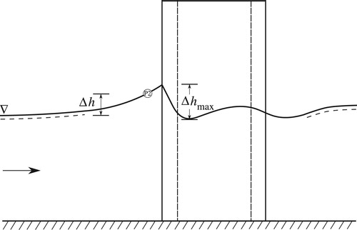As an example, the $\mathrm{\Delta }h$ at P2 is shown schematically in Fig. 3. As the flow approaches the pier, a free-surface roller is created. This elevates the free surface by up to 2 mm (Table 3). The free-surface height at the nose of the pier (Fig. 3) is expected to be even higher, but this location could not be measured in the experiment. At P2 and P3, the maximum variation in free surface is found and this corresponds to a value of $|\mathrm{\Delta }h|=3.39$ mm. Overall, the measured values and those obtained from the simulation are in good agreement, with the discrepancy between them being less than $10\mathrm{\%}$ at all four points.

Table 3. Elevation, ($\mathrm{\Delta }h$) of the free-surface around the pier for the experiment and simulation.

Location	Experiment (mm)	Simulation (mm)	Error ($\mathrm{\%}$)
$P1$	−0.84	−0.81	3.9
$P2$	2.16	1.98	8.3
$P3$	−1.13	−1.22	7.3
$P4$	−3.14	−3.39	7.3

Figure 3. Schematic description of free-surface variation for high Froude numbers

3.2. Flow field validation

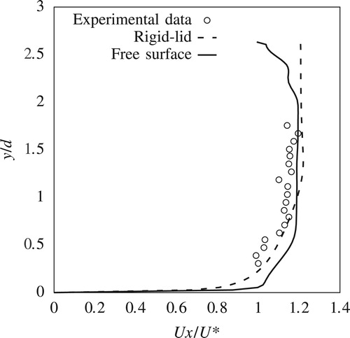
This paper compares only the streamwise components of the velocities from the experiment and the CFD simulations. Transverse and vertical components are not presented here for reasons of brevity. Figures 4 and 5 show streamwise velocity profiles at two upstream locations P1 and P2 (Fig. 2). Streamwise velocity results from both rigid-lid models and VOF models, which are from here on referred to as free-surface models, are plotted alongside the corresponding measured data. Figures 6 and 7 show similar plots for locations P3 and P4, which are to the side of the pier.

Figure 4. Experimental and numerical mean streamwise velocities at P1

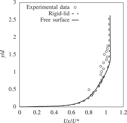
Figure 5. Experimental and numerical mean streamwise velocities at P2

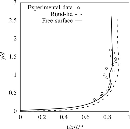
Figure 6. Experimental and numerical mean streamwise velocities at P3

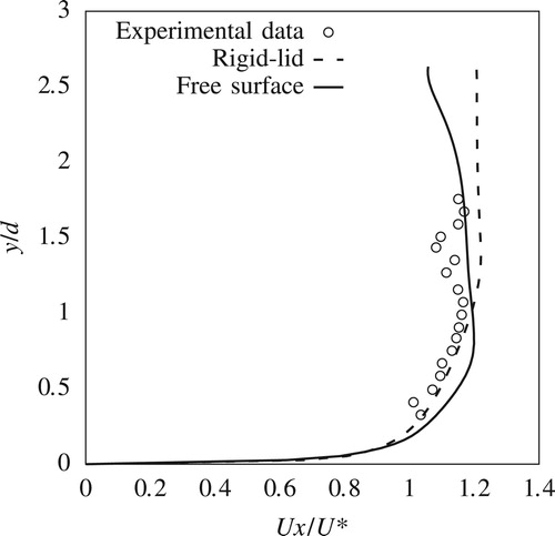
Figure 7. Experimental and numerical mean streamwise velocities at P4

Upstream of the pier at P1, there is good agreement between results from numerical simulations and measurements. Although there is a slight overestimation of the velocities for $1<y/d<1.5$, this discrepancy is well within the experimental error of the ADV. The comparison in Fig. 5 reveals the impact of the free-surface roller which contributes to the adverse pressure gradient along the front of the pier's nose and results in a global reduction of the horizontal velocity components. This effect is not captured in the rigid-lid simulation, which only experiences the shearing of the flow around the pier. Consequently, results from the free-surface model show much better agreement with the experiment than the rigid-lid simulations.

Around the side of the pier, within the shear layer, the free surface experiences a drop of 1.22 mm. This drop is reflected in the reduction in the streamwise velocity components for $y/d>1$ in the free-surface simulation (Figs 6 and 7) which is in agreement also with the measured data. However the rigid-lid simulation fails to capture this velocity reduction. For $y/d<1$, the prediction of the fully developed boundary layer is in good agreement with the measured data, with the discrepancy between the results from the rigid-lid and free-surface simulations being small.

Figures 8–11 compare the predicted and measured streamwise velocity components across the flow width (Section 2) in the downstream side of the pier. These plots show the mean recirculation zone behind the pier and how it decays downstream. Figures 8 and 9 illustrate that the free-surface drop behind the pier has a significant effect on the recirculation zone's length and magnitude. This drop is due to the pressure decrease behind the pier as a direct result of the strong recirculation zone. The rigid-lid simulations overestimate the streamwise velocity components, while predictions from the free-surface model match closely the measured velocity data. Figures 10 and 11 further confirm these findings although at these locations both the free surface and the rigid-lid simulations fail to match the measured streamwise velocity at the centreline of the flow ($w/d=0$). This is an expected result due to the inherent shortcomings of RANS modelling for predicting strong recirculating regions due to the assumption of isotropic Reynolds stress components.

Figure 8. Experimental and numerical velocity distribution downstream of the pier at 0.255w

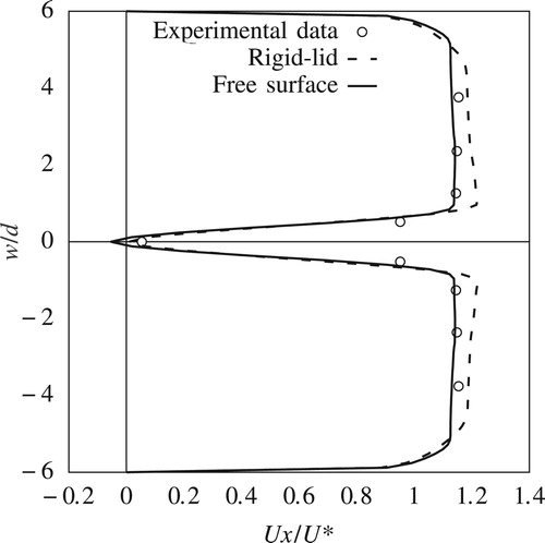
Figure 9. Experimental and numerical velocity distribution downstream of the pier at 0.338w

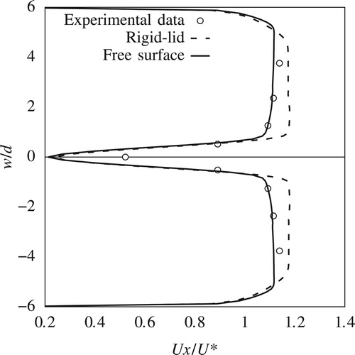
Figure 10. Experimental and numerical velocity distribution downstream of the pier at 0.4w

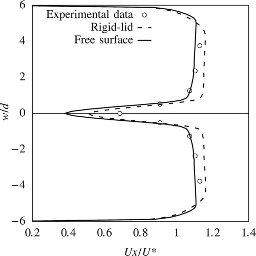
Figure 11. Experimental and numerical velocity distribution downstream of the pier at 0.455w

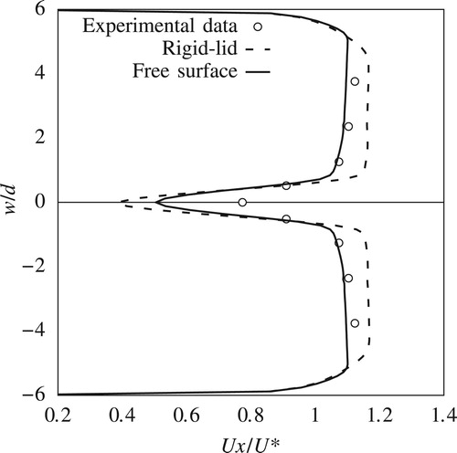
Figure 12 compares the predicted and measured turbulent kinetic energy (TKE) profiles. The plots show that the free surface can have a dramatic affect on the TKE distribution. For $y/d>1$, the TKE increases as we approach the free surface. This is a finding that is consistent with the experimental observations. However the rigid-lid simulation clearly underpredicts the TKE owing to the exclusion of the free surface and, therefore, gravity effects. Comparing these figures with Figs 8–11 reveals the reason for the velocity predictions from free-surface simulations showing a better agreement with experimental measurements. The increase in TKE over the region ($y/d>1$) extracts momentum from the mean flow and results in a slowing down. This behaviour, confirmed by the experimental data but absent in the rigid-lid simulations, is the main reason for the discrepancy between the velocity fields predicted by the free-surface and rigid-lid simulations.

Figure 12. Plots of TKE for P1, P2, P3 & P4, respectively. The solid and the dashed line represent data from the free-surface and rigid-lid simulations; the circles correspond to the measured data

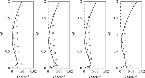
Figure 12 overall shows that the turbulence model underpredicts the TKE, especially in regions ($0.5<y/d<1$), and this may be due to an assumption made in the k-ω SST model. The TKE from experimental data is calculated as $k=0.5({u^{\prime }}^2+{v^{\prime }}^2+{w^{\prime }}^2)$, where $u^{\prime }$, $v^{\prime }$ and $w^{\prime }$ are the magnitudes of the fluctuating velocity components in the streamwise, transverse and vertical directions; the anisotropy in turbulence is accounted for using velocity components in all three directions. However, in the simulations, the Boussinesq approximation that underpins the k-ω turbulence model leads to k being computed as $k=1.5{u^{\prime }}^2$ by taking ${u^{\prime }}^2={v^{\prime }}^2={w^{\prime }}^2$ to ensure isotropy, a feature that is not present in experiments. The isotropic nature of the TKE can impinge on the production in the shear layer and the redistribution of the energy throughout its components and result in a reduction in the propagation of TKE across the whole flow depth.

3.3. Influence of Froude number

The free-surface variation around the pier, which affects the velocity components, is largely dictated by the Froude number, $\mathsf{F}\mathsf{=}{\mathsf{U}}^{\mathsf{\ast }}\mathsf{/}\sqrt{\mathsf{g}\mathsf{y}}$. In order to understand the relationship between the Froude number, the free surface and the velocities, four numerical simulations are conducted corresponding to $\mathsf{F}\mathsf{=}\mathsf{0.1}$, 0.2, 0.3 and 0.4. The model set-up is as outlined in Section 2 and identical to the models validated in Sections 3.1 and 3.2, except that the velocity at the inlet in each of these four simulations is adjusted to match the specific Froude number.

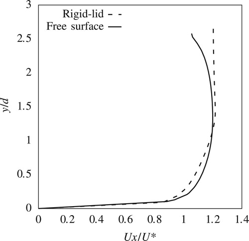
The free-surface profile at points P2 and P3 are chosen for investigation due to them being in the region where the free surface is expected to drop, as shown schematically in Fig. 3. The largest free-surface changes are found at P2 as shown in Table 4. This is also reflected in Figs 13–16 which show that, at P2, there are significant differences in the streamwise components of the flow velocities predicted using the free-surface and the rigid-lid simulations. Even for a Froude number as low as 0.1, the magnitudes of the velocities from the rigid-lid simulation are smaller than those from the free-surface simulation. The disparity between the predictions from the rigid-lid and free-surface simulations increases with further increase in the flow Froude number. This finding, as supported by the results in both Figs 13 and 14, is contrary to current assumptions (Graf & Yulistiyanto, 1998; Roulund et al., 2005) that the influence of the free surface variation on the flow field is negligible at small Froude numbers.

Figure 13. Comparison between rigid-lid and free-surface at P2, $\mathsf{F}\mathsf{=}\mathsf{0.1}$

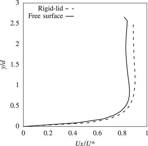
Figure 14. Comparison between rigid-lid and free-surface at P2, $\mathsf{F}\mathsf{=}\mathsf{0.2}$

Figure 15. Comparison between rigid-lid and free-surface at P2, $\mathsf{F}\mathsf{=}\mathsf{0.3}$

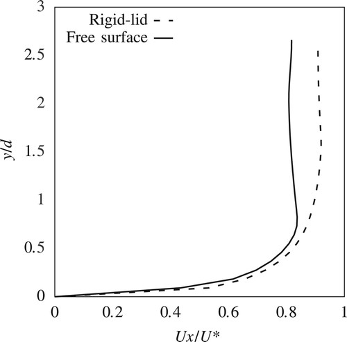
Figure 16. Comparison between rigid-lid and free-surface at P2, $\mathsf{F}\mathsf{=}\mathsf{0.4}$

Table 4. Elevation, ($\mathrm{\Delta }h$) of the simulated free-surface drop for different Froude numbers.

F	0.1	0.2	0.3	0.4
P2	0.3	1.145	1.9	2.03
P3	−0.25	−0.273	−0.88	−1.02
$\mathrm{\Delta }h$ (mm)	0.55	1.418	2.78	3.05

At P3 (Figs 17–20), the variation in the free surface relative to the approach flow is not as pronounced as at P2. Consequently, the differences between the velocities from the rigid-lid and free-surface simulations at P3 are also not as stark, especially for small Froude numbers (Figs 17 and 18). However, the magnitude of the free-surface drop does increase with the Froude number (Table 4) and so does the difference between the velocities from the rigid-lid and free surface simulations, as observed from Figs 17–20. In Fig. 19, the influence of the free surface on the flow field is evident for $y/d>1.5$; the drop in the free surface tends to slow down the flow near the free surface. This effect manifests itself more strongly for $\mathsf{F}\mathsf{=}\mathsf{0.4}$ in Fig. 20.

Figure 17. Comparison between rigid-lid and free-surface at P3, $\mathsf{F}\mathsf{=}\mathsf{0.1}$

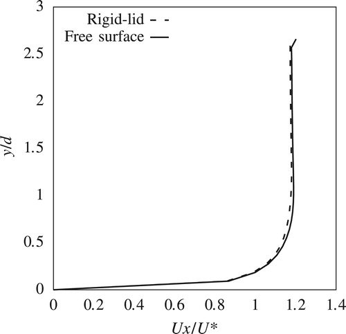
Figure 18. Comparison between rigid-lid and free-surface at P3, $\mathsf{F}\mathsf{=}\mathsf{0.2}$

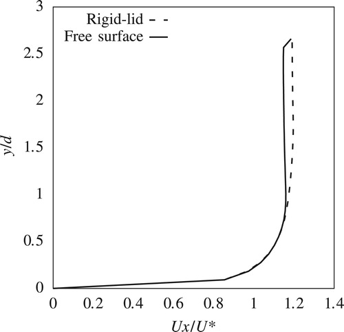
Figure 19. Comparison between rigid-lid and free-surface at P3, $\mathsf{F}\mathsf{=}\mathsf{0.3}$

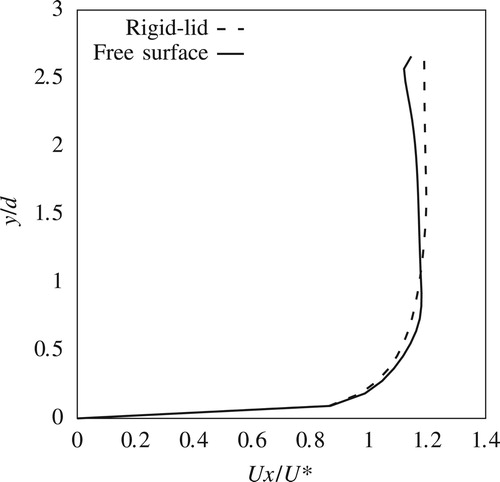
Figure 20. Comparison between rigid-lid and free-surface at P3, $\mathsf{F}\mathsf{=}\mathsf{0.4}$

3.4. Discussion

The streamwise velocity profile shown in Fig. 13 is obtained at location P2 for $\mathsf{F}\mathsf{=}\mathsf{0.1}$, which conforms to the $\mathsf{F}\le \mathsf{0.2}$ limit suggested for using the rigid lid assumption. The small change in free-surface height, i.e. a 0.22% increase in free-surface height relative to the approach flow, also appears to corroborate this currently accepted practice. However, further inspection of the results shows that the small free-surface variation still has a substantial impact on the flow field. Thus even for small Froude numbers, free-surface simulations may be required to capture accurately the local flow field around the pier. This finding is surprising particularly given the simulations in this study are performed using a sharp-nosed pier. In comparison to other pier geometries, this geometry is expected to have a lesser influence on the free surface due to its smaller frontal area and also experience a lower adverse pressure gradient.

The above finding can also support drawing significant inferences on the importance of free-surface modelling when investigating flow fields around blunt faced piers such as circular or square piers. Such geometries have a larger frontal area and are also likely to experience a higher adverse pressure gradient than the sharp-nosed piers. Consequently, these geometries, even for flows with small Froude numbers, may show a large free-surface variation (both roller and drop) and experience flow reversal at the base of the pier. As a result, free-surface simulations are essential for evaluating accurately the flow field in the vicinity of piers. Using a rigid-lid assumption may result in erroneous velocity predictions.

Lastly, the free-surface changes reported in this study are small - all less than 2% of the approach flow. However, this is largely due to the scale of the model which is designed to match the scale used in a laboratory experiment. If the simulations are run at full-scale for real-life bridge piers, the free-surface variations observed may be even larger and their influence on flow greater.

4. Conclusions

This paper presents findings from a numerical investigation of the free-surface variation and immediate flow field around a sharp-nosed pier for flows with various Froude numbers. The main conclusions are as follows:

1. A free-surface simulation using a VOF model within the open-source CFD toolbox OpenFOAM is able to accurately match the free-surface variation, the mean streamwise velocity and turbulent kinetic energy measured from the corresponding laboratory experiment.

2. The free-surface variation, even if small in comparison to the depth of the approach flow, has a significant influence on the TKE, and this leads to significant errors in TKE predictions for a simulation using a rigid-lid assumption.

3. Neglecting the hydro-static gradient due to the free-surface variation, even for flows with small Froude numbers ($\mathsf{F}\approx \mathsf{0.1}$), can lead to significant errors in the flow field predictions in the immediate vicinity of the pier.

4. For blunt-faced piers (e.g. circular and square piers) that have large adverse gradients, the influence of free surface on the flow field may be even more pronounced than for sharp-nosed piers due to a stronger free-surface roller and drop.

Notation

d	=	diameter of the pier $\left(\mathrm{m}\right)$
$\mathit{F}$	=	surface tension force $\left(\mathrm{k}\mathrm{g}{\mathrm{m}}^{-1}{\mathrm{s}}^{-2}\right)$
F	=	Froude number (–)
$\mathit{g}$	=	gravity $\left(\mathrm{m}{\mathrm{s}}^{-2}\right)$
k	=	turbulent kinetic energy $\left({\mathrm{m}}^2{\mathrm{s}}^{-2}\right)$
p	=	pressure $\left(\mathrm{k}\mathrm{g}{\mathrm{m}}^{-1}{\mathrm{s}}^{-2}\right)$
Q	=	discharge $\left({\mathrm{m}}^3{\mathrm{s}}^{-1}\right)$
R	=	Reynolds number $(-)$
$\mathbf{\text{{S}}}$	=	strain rate tensor $\left({\mathrm{s}}^{-1}\right)$
t	=	time (s)
${\mathrm{U}}^{\ast }$	=	centreline velocity $\left(\mathrm{m}{\mathrm{s}}^{-1}\right)$
$\mathit{U}$	=	velocity $\left(\mathrm{m}{\mathrm{s}}^{-1}\right)$
w	=	width of channel (m)
y	=	flow depth (m)
$u^{\prime },v^{\prime },w^{\prime }$	=	fluctuating velocity components in each direction respectively $\left({\mathrm{m}}^2{\mathrm{s}}^{-2}\right)$
α	=	volume fraction (–)
κ	=	free-surface curvature $\left({\mathrm{m}}^{-2}\right)$
μ	=	laminar viscosity $\left(\mathrm{k}\mathrm{g}{\mathrm{m}}^{-1}{\mathrm{s}}^{-1}\right)$
${\mu }_t$	=	turbulent viscosity $\left(\mathrm{k}\mathrm{g}{\mathrm{m}}^{-1}{\mathrm{s}}^{-1}\right)$
ρ	=	density of fluid $\left(\mathrm{k}\mathrm{g}{\mathrm{m}}^{-1}\right)$
σ	=	surface tension $\left(\mathrm{k}\mathrm{g}{\mathrm{m}}^2{\mathrm{s}}^{-2}\right)$
ω	=	specific rate of turbulence $\left({\mathrm{s}}^{-1}\right)$

Additional information

Funding

The research presented in this paper was supported by funding from the UK's Engineering and Physical Sciences Research Council (EPSRC) under grant EP/M017354/1. Data supporting the presented work can be accessed via the University of Exeter's data repository (https://doi.org/10.24378/exe.1503).

References

- Baranya, S., Olsen, N. R. B., Stoesser, T., & Sturm, T. (2012). Three-dimensional RANS modeling of flow around circular piers using nested grids. Engineering Applications of Computational Fluid Mechanics, 6(4), 648–662. doi: 10.1080/19942060.2012.11015449
- Baranya, S., Olsen, N. R. B., Stoesser, T., & Sturm, T. W. (2014). A nested grid based computational fluid dynamics model to predict bridge pier scour. Proceedings of the Institution of Civil Engineers: Water Management, 167(5), 259–268.
- Brackbill, J. U., Kothe, D. B., & Zemach, C. (1992). A continuum method for modeling surface tension. Journal of computational physics, 100(2), 335–354. doi: 10.1016/0021-9991(92)90240-Y
- Breusers, H. N. C., Nicollet, G., & Shen, H. W. (1977). Local scour around cylindrical piers. Journal of Hydraulic Research, 15(3), 211–252. doi: 10.1080/00221687709499645
- Burkow, M., & Griebel, M. (2016). A full three dimensional numerical simulation of the sediment transport and the scouring at a rectangular obstacle. Computers & Fluids, 125, 1–10. doi: 10.1016/j.compfluid.2015.10.014
- Chu, C.-R., Chung, C.-H., Wu, T.-R., & Wang, C.-Y. (2016). Numerical analysis of free surface flow over a submerged rectangular bridge deck. Journal of Hydraulic Engineering, 142(12), 04016060. doi: 10.1061/(ASCE)HY.1943-7900.0001177
- Ebrahimi, M., Kahraman, R., Kripakaran, P., Djordjević, S., Tabor, G., Prodanović, D., & Riella, M. (2017). Scour and hydrodynamic effects of debris blockage at masonry bridges: Insights from experimental and numerical modelling. In Aminuddin Ab. Ghani (Ed.), 37th IAHR World Conference. Kuala Lumpur, Malaysia: IAHR.
- Ebrahimi, M., Kripakaran, P., Prodanović, D., Kahraman, R., Riella, M., Tabor, G., & Djordjević, S. (2018). Experimental study on scour at a sharp-nose bridge pier with debris blockage. Journal of Hydraulic Engineering, 144(12), 04018071. doi: 10.1061/(ASCE)HY.1943-7900.0001516
- Ferziger, J. H., & Peric, M. (1996). Computational methods for fluid dynamics. Berlin: Springer Berlin Heidelberg.
- Graf, W. H., & Yulistiyanto, B. (1998). Experiments on flow around a cylinder; the velocity and vorticity fields. Journal of Hydraulic Research, 36(4), 637–654. doi: 10.1080/00221689809498613
- Huang, W., Yang, Q., & Xiao, H. (2009). CFD modeling of scale effects on turbulence flow and scour around bridge piers. Computers & Fluids, 38(5), 1050–1058. doi: 10.1016/j.compfluid.2008.01.029
- Issa, R. I. (1986). Solution of the implicitly discretised fluid flow equations by operator-splitting. Journal of Computational Physics, 62(1), 40–65. doi: 10.1016/0021-9991(86)90099-9
- Kang, S., & Sotiropoulos, F. (2015). Large-eddy simulation of three-dimensional turbulent free surface flow past a complex stream restoration structure. Journal of Hydraulic Engineering, 141(10), 04015022. doi: 10.1061/(ASCE)HY.1943-7900.0001034
- Kara, S., Kara, M. C., Stoesser, T., & Sturm, T. W. (2015). Free-surface versus rigid-lid les computations for bridge-abutment flow. Journal of Hydraulic Engineering, 141(9), 04015019. doi: 10.1061/(ASCE)HY.1943-7900.0001028
- Khosronejad, A., Kang, S., & Sotiropoulos, F. (2012). Experimental and computational investigation of local scour around bridge piers. Advances in Water Resources, 37, 73–85. doi: 10.1016/j.advwatres.2011.09.013
- Menter, F. R. (1994). Two-equation eddy-viscosity turbulence models for engineering applications. AIAA Journal, 32(8), 1598–1605. doi: 10.2514/3.12149
- Moukalled, F., Mangani, L., & Darwish, M. (2015). The finite volume method in computational fluid dynamics: An advanced introduction with openfoam and matlab (1st ed.). Springer, Incorporated. doi: 10.1007/978-3-319-16874-6
- Richardson, E. J., & Panchang, G. V. (1998). Three-Dimensional Simulation of Scour-Inducing Flow at Bridge Piers. Journal of Hydraulic Engineering, 124(5), 1–4. doi: 10.1061/(ASCE)0733-9429(1998)124:5(530)
- Richardson, J. F., & Zaki, W. N. (1997). Sedimentation and fluidisation: Part I. Chemical Engineering Research and Design, 75(3), S82–S100. doi: 10.1016/S0263-8762(97)80006-8
- Riella, M., Kahraman, R., & Tabor, G. R. (2018). Reynolds-averaged two-fluid model prediction of moderately dilute fluid-particle flow over a backward-facing step. International Journal of Multiphase Flow, 106, 95–108. doi: 10.1016/j.ijmultiphaseflow.2018.04.014
- Riella, M., Kahraman, R., & Tabor, G. R. (2019). Inhomogeneity and anisotropy in Eulerian-Eulerian near-wall modelling. International Journal of Multiphase Flow, 114, 9–18. doi: 10.1016/j.ijmultiphaseflow.2019.01.014
- Roulund, A., Sumer, B. M., Fredsoe, J., & Michelson, J. (2005). Numerical and experimental investigation of flow and scour around a circular pile. Journal of Fluid Mechanics, 534, 351–401. doi: 10.1017/S0022112005004507
- Sajedeh, H. A., Farsadizadeh, D., Arvanagh, H., & Abbaspour, A. (2016). Numerical Simulation of Flow Pattern around the Bridge Pier with Submerged Vanes. Journal of Hydraulic Structures, 2(2), 46–61.
- Versteeg, H. K., & Malalasekera, W. (1995). An introduction to computational fluid dynamics: The finite volume method. Harlow: Pearson Education Ltd.
- Weller, H. G., Tabor, G., Jasak, H., & Fureby, C. (1998). A tensorial approach to computational continuum mechanics using object-oriented techniques. Computers in Physics, 12(6), 620–631. doi: 10.1063/1.168744
- Zalesak, S. T. (1979). Fully multidimensional flux-corrected transport algorithms for fluids. Journal of Computational Physics, 31(3), 335–362. doi: 10.1016/0021-9991(79)90051-2