Double-averaged kinetic energy budgets in flows over mobile granular beds: insights from DNS data analysis

Abstract

The equations for double-mean, form-induced and spatially averaged turbulent energy budgets are employed to analyse data from direct numerical simulations of turbulent open-channel flows over transitionally rough mobile beds with intermediate flow submergence. Two scenarios were considered related to (i) near-critical bed condition, and (ii) fully mobile bed condition. The bed was composed of a layer of mobile spherical particles moving on the top of one layer of fixed particles of the same size. Data analysis showed the leading energy exchanges between double-mean, form-induced, turbulent flow field contributions as well as particle motions. Above the fixed particles tops, the turbulent flow receives kinetic energy directly from the mean flow as well as from moving bed particles, which in turn also receive energy from the mean flow. For near-critical bed condition, particle aggregations enhanced mean-flow heterogeneity, strengthened turbulent stresses and their effects on the flow, while at increased bed-mobility, energy transport mechanisms became weaker and conversions induced by viscous stresses and pressure became stronger.

Keywords:

• Double-averaging methodology
• flow–sediment interactions
• mean kinetic energy balance
• mobile-granular beds
• turbulent kinetic energy
• turbulent open-channel flows

1. Introduction

Sediment transport processes and the associated morphological changes to the river bed occur across a wide range of temporal and spatial scales (e.g. Dey, 2014; García, 2008; Graf & Altinakar, 1998; Julien, 2018). These scales vary from the scales of instantaneous movement of individual grains to the larger scales of bed formations manifested in the form of ripples, dunes, bars, meanders or anabranches. The role of sediment dynamics across these scales has been widely recognized and remains an important and active research area, with local and non-local scale interactions being among the key fundamental problems to be addressed (e.g. Ancey & Heyman, 2014; García, 2008; Singh, Foufoula-Georgiou, Porté-Angel, & Wilcock, 2012). To advance this problem, a procedure is needed for the transfer of information on fluid-mechanical and sediment transport processes from small scales (starting with a sub-grain scale) to larger scales. This transfer of information from smaller to larger scales is known as “upscaling”. The most physically appealing upscaling approach is based on the time and spatial averaging of the conservation equations for both fluid and sediments (e.g. Ballio, Nikora, & Coleman, 2014; Coleman & Nikora, 2009; Nikora, Ballio, Coleman, & Pokrajac, 2013). For example, spatial averaging of the Navier–Stokes equations for fluid within a thin horizontal slab with length and width comparable to flow depth represents upscaling of flow properties from the “point” scale to the depth scale. Similarly, combined time and spatial averaging, known as the double-averaging methodology (DAM), represents upscaling in both time and spatial domains (e.g. Giménez-Curto & Lera, 1996; Nikora, Goring, McEwan, & Griffiths, 2001; Pedras & de Lemos, 2001; Wilson & Shaw, 1977). DAM, and particularly the double-averaged forms of mass, momentum and kinetic energy balances, have been used increasingly in studies of atmospheric and water flows over fixed rough boundaries (e.g. Brunet, Finnigan, & Raupach, 1994; Coleman & Nikora, 2008; Dey & Das, 2012; Finnigan, 2000; Ghodke & Apte, 2016; Mignot, Barthelemy, & Hurther, 2009; Nikora et al., 2007b; Raupach & Shaw, 1982; Yuan & Piomelli, 2014). The averaging operation incorporates the effects of drag and flow heterogeneity (induced by the roughness geometry) in the equations of motion in the form of additional terms. Notable features of DAM include the consistent coupling of double-averaged variables, roughness geometry and bed shear stress, improved hydraulic definitions (such as flow uniformity and two-dimensionality), and possibilities for identification of specific flow layers and types as well as the partitioning of hydraulic resistance into mechanism-based contributions (Nikora, 2009; Nikora et al., 2007a, 2007b).

For the case of mobile rough boundaries, Nikora et al. (2013, 2007a) proposed refined definitions and theorems for double averaging, along with double-averaged equations for mass and momentum conservation for the fluid phase. These first-order equations are supplemented in a companion paper (Papadopoulos, Nikora, Cameron, Stewart, & Gibbins, 2019) with the second-order double-averaged equations describing the balances of the double-mean, form-induced and turbulent contributions to the total kinetic energy. Together with the mass and momentum conservation equations (Nikora et al., 2013), these energy conservation equations for mobile-bed flows represent a mathematical framework for physically-appealing upscaling, which in turn allows the assessment of interactions between mobile sediments and turbulent flow at different scales. Data for exploring the full potential of these equations (especially within moving roughness elements) are still limited and at present are mainly confined to particle-resolved direct numerical simulations (DNS; e.g. Chan-Braun, García-Villalba, & Uhlmann, 2011; Kempe, Vowinckel, & Fröhlich, 2014; Kidanemariam & Uhlmann, 2014; Soldati & Marchioli, 2012). Recent developments in refractive index matching particle image velocimetry are expected to soon also provide appropriately resolved experimental data. Assessments of the terms of the energy budgets using simulated and experimental data will help identify the most significant energy exchanges in mobile-bed flows and develop suitable models and parameterizations for predictions of sediment transport and turbulence characteristics.

Recently, Vowinckel, Nikora, Kempe, and Fröhlich (2017a, 2017b) applied the double-averaged momentum equations proposed in Nikora et al. (2013) to study flows over mobile rough beds using high-fidelity DNS data. Their work showed that bed mobility and heterogeneity can have significant effects on the flow, particularly within the roughness layer. The balances of the double mean, form-induced and spatially-averaged turbulent contributions to the fluid kinetic energy in mobile-bed flows can provide additional important insights, complementing findings of Dey and Das (2012), Mignot et al. (2009), Raupach and Shaw (1982) and Yuan and Piomelli (2014) obtained for fixed-bed conditions.

Against this background, the objective of this study was to identify the key energy exchanges involved in mobile-boundary flows by assessing the terms of the balance equations for double-mean kinetic energy (DMKE), form-induced kinetic energy (FKE) and spatially averaged turbulent kinetic energy (TKE). This assessment is based on the DNS dataset for turbulent open-channel flow over mobile-granular beds (Vowinckel et al., 2012) that was previously used for evaluation of the double-averaged momentum balance and momentum fluxes by Vowinckel et al. (2017a, 2017b).

The next section outlines the computational set-up and provides a brief overview of the double-averaging methodology. The assessment of the terms involved in the equations for the DMKE, FKE and spatially averaged turbulent energy are presented in Section 3, followed by the discussion of the results in Section 4. The conclusions are given in Section 5.

2. Numerical simulations, background equations and data analysis

The numerical model used in this study implements a partitioned approach for the simulation of the flow interactions with moving bed particles, where the fluid and particle dynamics are considered following the Eulerian and Lagrangian descriptions of motion, respectively. Their coupling is modelled through the immersed boundary method (IBM). A detailed description of the model's implementation of the IBM can be found in Uhlmann (2005) and Kempe and Fröhlich (2012b), while the discretization scheme and the solver are reported in Kempe and Fröhlich (2012a), and Kempe et al. (2014). The particle collision model for the simulation of particle motion is discussed in Kempe and Fröhlich (2012b) and Kempe et al. (2014). Complete details of the computational set-up and simulation scenarios are given in Vowinckel et al. (2012) and Vowinckel and Fröhlich (2012). Therefore, Section 2.1 describes the computational set-up and key physical parameters associated with the flow simulations used in this study only briefly.

2.1. Computational set-up

Two scenarios of turbulent open-channel flows over mobile granular beds were reproduced by DNS (Vowinckel & Fröhlich, 2012; Vowinckel et al., 2012). In both scenarios, the bed is composed of three components: a flat impermeable surface; a single layer of 6696 fixed spherical particles placed on this surface in hexagonal packing; and a layer of 2000 mobile spherical particles, which are free to move on the surface of the fixed particles. Both fixed and mobile particles have the same diameter D. The bulk and friction Reynolds numbers have been selected to be ${\text{R}}_{\text{b}}=U_{b}H/{\nu }_f=2700$ and ${\text{R}}_{\text{τ}}=u_{\tau }H/{\nu }_f=177$, respectively, where $U_b$ is the bulk velocity of the unladen flow, $u_{\tau }$ is the friction velocity, H is the flow depth and ${\nu }_f$ is the fluid kinematic viscosity. The flow depth H is defined as the distance from the tops of fixed particles to the water surface (i.e. the upper boundary of the computational domain). The computational domain is a rectangular volume whose streamwise, spanwise and bed-normal extents are $0\le x_1\le 12H$, $0\le x_2\le 6H$ and $-D\le x_3\le H$, where $x_1$, $x_2$, and $x_3$ are the streamwise, spanwise and bed-normal coordinates. Space coordinates are specified using a left-handed Cartesian system. The origins of the spanwise and bed-normal coordinates are placed at the left boundary of the domain and at the top of the fixed particles, respectively. The selection of the domain dimensions satisfies the requirement for reproducing most of the spectrum of turbulent eddies that scale with flow depth H (Vowinckel et al., 2017a). The domain is discretized using a uniform grid of $2400\times 1206\times 223$ cells with resolution $\mathrm{\Delta }{z}^{+}=u_{\tau }\mathrm{\Delta }z/{\nu }_f=0.86$, where $\mathrm{\Delta }z$ is the cell grid size. Hence, the spatial discretization is fine enough to resolve the viscous length scale ${\nu }_f/u_{\tau }$. The ratio of the particle diameter D to the grid cell size is $D/\mathrm{\Delta }z=22.2$, and thus the flow around fixed and mobile particles is fully resolved. The relative submergence $H/D=9$ and the roughness Reynolds number $D^{+}=u_{\tau }D/{\nu }_f=19.2$ are kept the same for all simulations, and thus the simulated flows can be considered as transitionally rough bed flows at intermediate submergence. The periodic boundary conditions are chosen for both streamwise and spanwise directions (for both the flow and moving particles). The no-slip condition is applied at the flat bottom boundary (supporting fixed particles) and at the particle–fluid interfacial surfaces while at the upper boundary (water surface) of the domain the slip-free condition is imposed.

Bed mobility was adjusted by modifying the particle specific density ${\rho }^{\mathrm{\prime }}=({\rho }_p-{\rho }_f)/{\rho }_f$, where ${\rho }_p$ and ${\rho }_f$ denote the particle and fluid mass densities, respectively. Different particle specific densities ${\rho }^{\mathrm{\prime }}$ correspond to different values of the Shields parameter $\text{Sh}=u_{\tau }^2/\left({\rho }^{\mathrm{\prime }}gD\right)$, where g is gravity acceleration. The ratio of the actual $\text{Sh}$ to the critical value ${\text{Sh}}_{\text{crit}}$ is used to characterize bed mobility. Two scenarios with different ratios $\text{Sh}/{\text{Sh}}_{\text{crit}}$ were studied. The first scenario corresponds to near-critical condition at the bed with specific density ${\rho }^{\mathrm{\prime }}=1.15$ and Shields number $\text{Sh}=0.024$ ($\text{Sh}/{\text{Sh}}_{\text{crit}}=0.7$); this is referred to as the “heavy particles” (HP) scenario. The second scenario had a lower specific density ${\rho }^{\mathrm{\prime }}=1.05$ and corresponds to fully mobile bed condition with $\text{Sh}=0.075$ ($\text{Sh}/{\text{Sh}}_{\text{crit}}=2.2$); this is referred to as the “light particles” (LP) scenario. The bedload transport rate for the second scenario was four times larger than that of the first (Vowinckel et al., 2017b). The flow data used for the present analysis are collected from the time instant after which statistically steady state conditions are established for particle motion (Vowinckel, Kempe, & Fröhlich, 2013). A comprehensive description of the computational set-up can be found in Vowinckel and Fröhlich (2012) and Vowinckel, Kempe, and Fröhlich (2014).

2.2. Double-averaged quantities and energy equations

For consecutive time-spatial averaging, the intrinsic ($⟨\overline{\theta }⟩$) and superficial ($⟨{\overline{\theta }}^s{⟩}^s$) double averages of a variable θ (e.g. fluid velocity or pressure) are defined as (Nikora et al., 2013): (1) $\begin{array}{rl}⟨\overline{\theta }⟩& =\frac{1}{V_m}{\int }_{V_0}\frac{1}{T_f}{\int }_{T_0}\theta (x_i,t)\gamma (x_i,t)\mathrm{d}t\mathrm{d}V,\\ ⟨{\overline{\theta }}^s{⟩}^s& =\frac{1}{V_0}{\int }_{V_0}\frac{1}{T_0}{\int }_{T_0}\theta (x_i,t)\gamma (x_i,t)\mathrm{d}t\mathrm{d}V\end{array}$(1) where the overbar and angular brackets denote time and spatial averaging, respectively; the superscript s denotes superficial type of averaging; $V_m$ is a part of the total averaging domain of volume $V_0$ that has been visited by the fluid at least once within the total averaging time $T_0$; and $T_f$ is the total time period within $T_0$ when a point within a spatial averaging domain was occupied by fluid, not necessarily continuously; $x_i$ is the position coordinate in the ith direction and γ is the distribution function that is equal to 1 when the point is occupied by the fluid and 0 otherwise. The ratios $T_f/T_0$ and $V_m/V_0$ define the local time porosity ${\phi }_T$ and the space porosity ${\phi }_{Vm}$, respectively, which are indicative of the bed roughness mobility and geometry. Their combination defines the space-time porosity ${\phi }_{VT}={\phi }_{Vm}⟨{\phi }_T⟩$. Intrinsic and superficial double-averaged quantities are linked through the relation $⟨{\overline{\theta }}^s{⟩}^s={\phi }_{Vm}⟨{\phi }_T\overline{\theta }⟩$ (Nikora et al., 2013).

The selection of the size and shape of the time-space averaging domain depends on the turbulence structure, bed roughness geometry and spatio-temporal variations of the mean flow (Nikora et al., 2007a). The averaging time $T_0$ should be much smaller than the characteristic time scale of the mean flow (e.g. flood duration for channel flows) and exceed the characteristic time scale of turbulent fluctuations (e.g. ratio of the flow depth to the flow velocity). In regard with the time scales of the roughness mobility, $T_0$ should be larger than the characteristic time scale of roughness elements motion (e.g. motion of individual sediment grains) and smaller than the time scales of the changes in bed morphology (e.g. development and evolution of bed forms). An appropriate shape of the spatial averaging domain is a thin slice parallel to the mean bed, with a vertical extent much smaller than the average roughness height. The bed-parallel dimensions of the averaging domain should be much larger than the roughness length scales along and across the flow but be much smaller than channel-scale of bed level fluctuations. A wide separation between the characteristic roughness scales and the scale of variation of the spatially-averaged value is required for spatial averaging conditions to hold.

The instantaneous velocity vector $u_i$ can be decomposed into a time-averaged value ${\overline{u}}_i$ and a fluctuation $u_i^{\mathrm{\prime }}$ such that $u_i={\overline{u}}_i+u_i^{\mathrm{\prime }}$, known as the Reynolds decomposition. Consequently, the total time-averaged fluid kinetic energy ($\frac{1}{2}\overline{u_i{u}_i}$, I in Eq. 2(2) $\begin{array}{rl}\underset{\mathrm{I}}{\underbrace{\frac{1}{2}{\phi }_{Vm}⟨{\phi }_T\overline{u_i{u}_i}⟩}}& =\underset{\mathrm{I}\mathrm{I}:\mathrm{M}\mathrm{K}\mathrm{E}}{\underbrace{\frac{1}{2}{\phi }_{Vm}⟨{\phi }_T{\overline{u}}_i{\overline{u}}_i⟩}}+\underset{\mathrm{I}\mathrm{I}\mathrm{I}:\mathrm{T}\mathrm{K}\mathrm{E}}{\underbrace{\frac{1}{2}{\phi }_{Vm}⟨{\phi }_T\overline{u_i^{\mathrm{\prime }}{u}_i^{\mathrm{\prime }}}⟩}}\\ & =\underset{\mathrm{I}\mathrm{I}\mathrm{A}\mathrm{B}:\mathrm{D}\mathrm{M}\mathrm{K}\mathrm{E}}{\underbrace{\underset{\mathrm{I}\mathrm{I}\mathrm{A}}{\underbrace{\frac{1}{2}{\phi }_{Vm}⟨{\overline{u}}_i⟩⟨{\overline{u}}_i⟩}}+\underset{\mathrm{I}\mathrm{I}\mathrm{B}}{\underbrace{\frac{1}{2}{\phi }_{Vm}⟨{\phi }_T{\tilde{\overline{u}}}_i⟩⟨{\overline{u}}_i⟩}}}}\\ & +\underset{\mathrm{I}\mathrm{I}\mathrm{C}:\mathrm{F}\mathrm{K}\mathrm{E}}{\underbrace{\frac{1}{2}{\phi }_{Vm}⟨{\phi }_T{\tilde{\overline{u}}}_i{\tilde{\overline{u}}}_i⟩}}+\underset{\mathrm{I}\mathrm{I}\mathrm{I}:\mathrm{T}\mathrm{K}\mathrm{E}}{\underbrace{\frac{1}{2}{\phi }_{Vm}⟨{\phi }_T\overline{u_i^{\mathrm{\prime }}{u}_i^{\mathrm{\prime }}}⟩}}\end{array}$(2) ) can be decomposed into contributions from the mean ($\frac{1}{2}{\overline{u}}_i{\overline{u}}_i$ , II in Eq. 2(2) $\begin{array}{rl}\underset{\mathrm{I}}{\underbrace{\frac{1}{2}{\phi }_{Vm}⟨{\phi }_T\overline{u_i{u}_i}⟩}}& =\underset{\mathrm{I}\mathrm{I}:\mathrm{M}\mathrm{K}\mathrm{E}}{\underbrace{\frac{1}{2}{\phi }_{Vm}⟨{\phi }_T{\overline{u}}_i{\overline{u}}_i⟩}}+\underset{\mathrm{I}\mathrm{I}\mathrm{I}:\mathrm{T}\mathrm{K}\mathrm{E}}{\underbrace{\frac{1}{2}{\phi }_{Vm}⟨{\phi }_T\overline{u_i^{\mathrm{\prime }}{u}_i^{\mathrm{\prime }}}⟩}}\\ & =\underset{\mathrm{I}\mathrm{I}\mathrm{A}\mathrm{B}:\mathrm{D}\mathrm{M}\mathrm{K}\mathrm{E}}{\underbrace{\underset{\mathrm{I}\mathrm{I}\mathrm{A}}{\underbrace{\frac{1}{2}{\phi }_{Vm}⟨{\overline{u}}_i⟩⟨{\overline{u}}_i⟩}}+\underset{\mathrm{I}\mathrm{I}\mathrm{B}}{\underbrace{\frac{1}{2}{\phi }_{Vm}⟨{\phi }_T{\tilde{\overline{u}}}_i⟩⟨{\overline{u}}_i⟩}}}}\\ & +\underset{\mathrm{I}\mathrm{I}\mathrm{C}:\mathrm{F}\mathrm{K}\mathrm{E}}{\underbrace{\frac{1}{2}{\phi }_{Vm}⟨{\phi }_T{\tilde{\overline{u}}}_i{\tilde{\overline{u}}}_i⟩}}+\underset{\mathrm{I}\mathrm{I}\mathrm{I}:\mathrm{T}\mathrm{K}\mathrm{E}}{\underbrace{\frac{1}{2}{\phi }_{Vm}⟨{\phi }_T\overline{u_i^{\mathrm{\prime }}{u}_i^{\mathrm{\prime }}}⟩}}\end{array}$(2) ) and turbulent ($\frac{1}{2}\overline{u_i^{\mathrm{\prime }}{u}_i^{\mathrm{\prime }}}$, III in Eq. 2(2) $\begin{array}{rl}\underset{\mathrm{I}}{\underbrace{\frac{1}{2}{\phi }_{Vm}⟨{\phi }_T\overline{u_i{u}_i}⟩}}& =\underset{\mathrm{I}\mathrm{I}:\mathrm{M}\mathrm{K}\mathrm{E}}{\underbrace{\frac{1}{2}{\phi }_{Vm}⟨{\phi }_T{\overline{u}}_i{\overline{u}}_i⟩}}+\underset{\mathrm{I}\mathrm{I}\mathrm{I}:\mathrm{T}\mathrm{K}\mathrm{E}}{\underbrace{\frac{1}{2}{\phi }_{Vm}⟨{\phi }_T\overline{u_i^{\mathrm{\prime }}{u}_i^{\mathrm{\prime }}}⟩}}\\ & =\underset{\mathrm{I}\mathrm{I}\mathrm{A}\mathrm{B}:\mathrm{D}\mathrm{M}\mathrm{K}\mathrm{E}}{\underbrace{\underset{\mathrm{I}\mathrm{I}\mathrm{A}}{\underbrace{\frac{1}{2}{\phi }_{Vm}⟨{\overline{u}}_i⟩⟨{\overline{u}}_i⟩}}+\underset{\mathrm{I}\mathrm{I}\mathrm{B}}{\underbrace{\frac{1}{2}{\phi }_{Vm}⟨{\phi }_T{\tilde{\overline{u}}}_i⟩⟨{\overline{u}}_i⟩}}}}\\ & +\underset{\mathrm{I}\mathrm{I}\mathrm{C}:\mathrm{F}\mathrm{K}\mathrm{E}}{\underbrace{\frac{1}{2}{\phi }_{Vm}⟨{\phi }_T{\tilde{\overline{u}}}_i{\tilde{\overline{u}}}_i⟩}}+\underset{\mathrm{I}\mathrm{I}\mathrm{I}:\mathrm{T}\mathrm{K}\mathrm{E}}{\underbrace{\frac{1}{2}{\phi }_{Vm}⟨{\phi }_T\overline{u_i^{\mathrm{\prime }}{u}_i^{\mathrm{\prime }}}⟩}}\end{array}$(2) ) fields, i.e. $\frac{1}{2}\overline{u_i{u}_i}=\frac{1}{2}{\overline{u}}_i{\overline{u}}_i+\frac{1}{2}\overline{u_i^{\mathrm{\prime }}{u}_i^{\mathrm{\prime }}}$ (repeated indices imply summation involving all three velocity components). For rough-bed flows, the time-averaged velocity can be further decomposed into a double-mean value $⟨{\overline{u}}_i⟩$ and a spatial fluctuation ${\tilde{\overline{u}}}_i$ such that ${\overline{u}}_i=⟨{\overline{u}}_i⟩+{\tilde{\overline{u}}}_i$. Then, the mean energy (II) can be decomposed into contributions from the double-mean velocity field $⟨{\overline{u}}_i⟩$ (IIA), contributions due to potential correlations between the time porosity and time-averaged fields (IIB), and contributions from the form-induced velocity field ${\tilde{\overline{u}}}_i$ (IIC), i.e.: (2) $\begin{array}{rl}\underset{\mathrm{I}}{\underbrace{\frac{1}{2}{\phi }_{Vm}⟨{\phi }_T\overline{u_i{u}_i}⟩}}& =\underset{\mathrm{I}\mathrm{I}:\mathrm{M}\mathrm{K}\mathrm{E}}{\underbrace{\frac{1}{2}{\phi }_{Vm}⟨{\phi }_T{\overline{u}}_i{\overline{u}}_i⟩}}+\underset{\mathrm{I}\mathrm{I}\mathrm{I}:\mathrm{T}\mathrm{K}\mathrm{E}}{\underbrace{\frac{1}{2}{\phi }_{Vm}⟨{\phi }_T\overline{u_i^{\mathrm{\prime }}{u}_i^{\mathrm{\prime }}}⟩}}\\ & =\underset{\mathrm{I}\mathrm{I}\mathrm{A}\mathrm{B}:\mathrm{D}\mathrm{M}\mathrm{K}\mathrm{E}}{\underbrace{\underset{\mathrm{I}\mathrm{I}\mathrm{A}}{\underbrace{\frac{1}{2}{\phi }_{Vm}⟨{\overline{u}}_i⟩⟨{\overline{u}}_i⟩}}+\underset{\mathrm{I}\mathrm{I}\mathrm{B}}{\underbrace{\frac{1}{2}{\phi }_{Vm}⟨{\phi }_T{\tilde{\overline{u}}}_i⟩⟨{\overline{u}}_i⟩}}}}\\ & +\underset{\mathrm{I}\mathrm{I}\mathrm{C}:\mathrm{F}\mathrm{K}\mathrm{E}}{\underbrace{\frac{1}{2}{\phi }_{Vm}⟨{\phi }_T{\tilde{\overline{u}}}_i{\tilde{\overline{u}}}_i⟩}}+\underset{\mathrm{I}\mathrm{I}\mathrm{I}:\mathrm{T}\mathrm{K}\mathrm{E}}{\underbrace{\frac{1}{2}{\phi }_{Vm}⟨{\phi }_T\overline{u_i^{\mathrm{\prime }}{u}_i^{\mathrm{\prime }}}⟩}}\end{array}$(2) The contributions (IIAB), (IIC) and (III) are referred to as the DMKE, FKE and spatially averaged TKE, respectively. Equations describing the balances of the DMKE, FKE and TKE in mobile-bed flows, proposed in Papadopoulos et al. (2019, therein eqs 17, 19 and 21), can provide important insights into the mechanisms of energy generation, exchanges, transport and dissipation. The present paper is a follow-up of Papadopoulos et al. (2019) as it provides assessments of the terms involved in the budgets of DMKE, FKE and TKE (Section 3) as well as it discusses their physical significance (Sections 4 and 5).

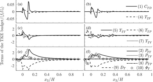
2.2.1. Balance of the double-mean energy

Due to the computational set-up in the employed DNS, the time-averaged field is considered as steady and thus the time derivatives vanish, leading to the budget of the DMKE (term IIAB in Eq. 2(2) $\begin{array}{rl}\underset{\mathrm{I}}{\underbrace{\frac{1}{2}{\phi }_{Vm}⟨{\phi }_T\overline{u_i{u}_i}⟩}}& =\underset{\mathrm{I}\mathrm{I}:\mathrm{M}\mathrm{K}\mathrm{E}}{\underbrace{\frac{1}{2}{\phi }_{Vm}⟨{\phi }_T{\overline{u}}_i{\overline{u}}_i⟩}}+\underset{\mathrm{I}\mathrm{I}\mathrm{I}:\mathrm{T}\mathrm{K}\mathrm{E}}{\underbrace{\frac{1}{2}{\phi }_{Vm}⟨{\phi }_T\overline{u_i^{\mathrm{\prime }}{u}_i^{\mathrm{\prime }}}⟩}}\\ & =\underset{\mathrm{I}\mathrm{I}\mathrm{A}\mathrm{B}:\mathrm{D}\mathrm{M}\mathrm{K}\mathrm{E}}{\underbrace{\underset{\mathrm{I}\mathrm{I}\mathrm{A}}{\underbrace{\frac{1}{2}{\phi }_{Vm}⟨{\overline{u}}_i⟩⟨{\overline{u}}_i⟩}}+\underset{\mathrm{I}\mathrm{I}\mathrm{B}}{\underbrace{\frac{1}{2}{\phi }_{Vm}⟨{\phi }_T{\tilde{\overline{u}}}_i⟩⟨{\overline{u}}_i⟩}}}}\\ & +\underset{\mathrm{I}\mathrm{I}\mathrm{C}:\mathrm{F}\mathrm{K}\mathrm{E}}{\underbrace{\frac{1}{2}{\phi }_{Vm}⟨{\phi }_T{\tilde{\overline{u}}}_i{\tilde{\overline{u}}}_i⟩}}+\underset{\mathrm{I}\mathrm{I}\mathrm{I}:\mathrm{T}\mathrm{K}\mathrm{E}}{\underbrace{\frac{1}{2}{\phi }_{Vm}⟨{\phi }_T\overline{u_i^{\mathrm{\prime }}{u}_i^{\mathrm{\prime }}}⟩}}\end{array}$(2) ) being: (3) $\begin{array}{rl}& \underset{\left(1\right):C_{DD}}{\underbrace{\frac{1}{2}\frac{\mathrm{\partial }}{\mathrm{\partial }{x}_j}({\phi }_{VT}⟨{\overline{u}}_i⟩⟨{\overline{u}}_i⟩⟨{\overline{u}}_j⟩)}}+\underset{\left(2\right):C_{DM}}{\underbrace{\frac{\mathrm{\partial }}{\mathrm{\partial }{x}_j}({\phi }_{Vm}⟨{\phi }_T{\tilde{\overline{u}}}_i⟩⟨{\overline{u}}_i⟩⟨{\overline{u}}_j⟩)}}\\ & =\underset{\left(3\right):G_D}{\underbrace{{\phi }_{VT}⟨{\overline{u}}_1⟩f_1}}-\underset{\left(4\right):-T_{DT}}{\underbrace{\frac{\mathrm{\partial }}{\mathrm{\partial }{x}_j}({\phi }_{Vm}⟨{\phi }_T\overline{u_i^{\mathrm{\prime }}{u}_j^{\mathrm{\prime }}}⟩⟨{\overline{u}}_i⟩)}}\\ & -\underset{\left(5\right):-T_{DF}}{\underbrace{\frac{\mathrm{\partial }}{\mathrm{\partial }{x}_j}({\phi }_{Vm}⟨{\phi }_T{\tilde{\overline{u}}}_i{\tilde{\overline{u}}}_j⟩⟨{\overline{u}}_i⟩)}}-\underset{\left(6\right):-T_{DM}}{\underbrace{\frac{1}{2}\frac{\mathrm{\partial }}{\mathrm{\partial }{x}_j}({\phi }_{Vm}⟨{\phi }_T{\tilde{\overline{u}}}_j⟩⟨{\overline{u}}_i⟩⟨{\overline{u}}_i⟩)}}\\ & -\underset{\left(7\right):-T_{DP}}{\underbrace{\frac{1}{{\rho }_f}\frac{\mathrm{\partial }}{\mathrm{\partial }{x}_i}({\phi }_{Vm}⟨{\phi }_T\overline{p}⟩⟨{\overline{u}}_i⟩)}}+\underset{\left(8\right):T_{DV}}{\underbrace{{\nu }_f\frac{\mathrm{\partial }}{\mathrm{\partial }{x}_j}({\phi }_{Vm}⟨{\phi }_T\overline{\frac{\mathrm{\partial }{u}_i}{\mathrm{\partial }{x}_j}}⟩⟨{\overline{u}}_i⟩)}}\\ & +\underset{\left(9\right):P_{DT}}{\underbrace{{\phi }_{Vm}⟨{\phi }_T\overline{u_i^{\mathrm{\prime }}{u}_j^{\mathrm{\prime }}}⟩\frac{\mathrm{\partial }⟨{\overline{u}}_i⟩}{\mathrm{\partial }{x}_j}}}+\underset{\left(10\right):P_{DF}}{\underbrace{{\phi }_{Vm}⟨{\phi }_T{\tilde{\overline{u}}}_i{\tilde{\overline{u}}}_j⟩\frac{\mathrm{\partial }⟨{\overline{u}}_i⟩}{\mathrm{\partial }{x}_j}}}\\ & +\underset{\left(11\right):P_{DM}}{\underbrace{{\phi }_{Vm}⟨{\phi }_T{\tilde{\overline{u}}}_i⟩⟨{\overline{u}}_j⟩\frac{\mathrm{\partial }⟨{\overline{u}}_i⟩}{\mathrm{\partial }{x}_j}}}\\ & +\underset{\left(12\right):P_{DP}}{\underbrace{\frac{{\phi }_{Vm}⟨{\phi }_T\overline{p}⟩}{{\rho }_f}\frac{\mathrm{\partial }⟨{\overline{u}}_i⟩}{\mathrm{\partial }{x}_i}}}-\underset{\left(13\right):-D_D}{\underbrace{{\nu }_f{\phi }_{Vm}⟨{\phi }_T\overline{\frac{\mathrm{\partial }{u}_i}{\mathrm{\partial }{x}_j}}⟩\frac{\mathrm{\partial }⟨{\overline{u}}_i⟩}{\mathrm{\partial }{x}_j}}}\\ & +\underset{\left(14\right):{\Phi }_D}{\underbrace{\frac{⟨{\overline{u}}_i⟩}{{\rho }_f{V}_0}{\overline{{\int }_{S_{int}}p{n}_i\mathrm{d}S}}^s-\frac{⟨{\overline{u}}_i⟩}{V_0}{\overline{{\int }_{S_{int}}{\nu }_f\frac{\mathrm{\partial }{u}_i}{\mathrm{\partial }{x}_j}{n}_j\mathrm{d}S}}^s}}\end{array}$(3) where $f_1$ is a volume force driving the flow (it represents the gravity effect), p is fluid pressure and $n_j$ is the unit vector normal to the interfacial surface $S_{int}$ and directed into the fluid. Terms 1 and 2 in Eq. (3(3) $\begin{array}{rl}& \underset{\left(1\right):C_{DD}}{\underbrace{\frac{1}{2}\frac{\mathrm{\partial }}{\mathrm{\partial }{x}_j}({\phi }_{VT}⟨{\overline{u}}_i⟩⟨{\overline{u}}_i⟩⟨{\overline{u}}_j⟩)}}+\underset{\left(2\right):C_{DM}}{\underbrace{\frac{\mathrm{\partial }}{\mathrm{\partial }{x}_j}({\phi }_{Vm}⟨{\phi }_T{\tilde{\overline{u}}}_i⟩⟨{\overline{u}}_i⟩⟨{\overline{u}}_j⟩)}}\\ & =\underset{\left(3\right):G_D}{\underbrace{{\phi }_{VT}⟨{\overline{u}}_1⟩f_1}}-\underset{\left(4\right):-T_{DT}}{\underbrace{\frac{\mathrm{\partial }}{\mathrm{\partial }{x}_j}({\phi }_{Vm}⟨{\phi }_T\overline{u_i^{\mathrm{\prime }}{u}_j^{\mathrm{\prime }}}⟩⟨{\overline{u}}_i⟩)}}\\ & -\underset{\left(5\right):-T_{DF}}{\underbrace{\frac{\mathrm{\partial }}{\mathrm{\partial }{x}_j}({\phi }_{Vm}⟨{\phi }_T{\tilde{\overline{u}}}_i{\tilde{\overline{u}}}_j⟩⟨{\overline{u}}_i⟩)}}-\underset{\left(6\right):-T_{DM}}{\underbrace{\frac{1}{2}\frac{\mathrm{\partial }}{\mathrm{\partial }{x}_j}({\phi }_{Vm}⟨{\phi }_T{\tilde{\overline{u}}}_j⟩⟨{\overline{u}}_i⟩⟨{\overline{u}}_i⟩)}}\\ & -\underset{\left(7\right):-T_{DP}}{\underbrace{\frac{1}{{\rho }_f}\frac{\mathrm{\partial }}{\mathrm{\partial }{x}_i}({\phi }_{Vm}⟨{\phi }_T\overline{p}⟩⟨{\overline{u}}_i⟩)}}+\underset{\left(8\right):T_{DV}}{\underbrace{{\nu }_f\frac{\mathrm{\partial }}{\mathrm{\partial }{x}_j}({\phi }_{Vm}⟨{\phi }_T\overline{\frac{\mathrm{\partial }{u}_i}{\mathrm{\partial }{x}_j}}⟩⟨{\overline{u}}_i⟩)}}\\ & +\underset{\left(9\right):P_{DT}}{\underbrace{{\phi }_{Vm}⟨{\phi }_T\overline{u_i^{\mathrm{\prime }}{u}_j^{\mathrm{\prime }}}⟩\frac{\mathrm{\partial }⟨{\overline{u}}_i⟩}{\mathrm{\partial }{x}_j}}}+\underset{\left(10\right):P_{DF}}{\underbrace{{\phi }_{Vm}⟨{\phi }_T{\tilde{\overline{u}}}_i{\tilde{\overline{u}}}_j⟩\frac{\mathrm{\partial }⟨{\overline{u}}_i⟩}{\mathrm{\partial }{x}_j}}}\\ & +\underset{\left(11\right):P_{DM}}{\underbrace{{\phi }_{Vm}⟨{\phi }_T{\tilde{\overline{u}}}_i⟩⟨{\overline{u}}_j⟩\frac{\mathrm{\partial }⟨{\overline{u}}_i⟩}{\mathrm{\partial }{x}_j}}}\\ & +\underset{\left(12\right):P_{DP}}{\underbrace{\frac{{\phi }_{Vm}⟨{\phi }_T\overline{p}⟩}{{\rho }_f}\frac{\mathrm{\partial }⟨{\overline{u}}_i⟩}{\mathrm{\partial }{x}_i}}}-\underset{\left(13\right):-D_D}{\underbrace{{\nu }_f{\phi }_{Vm}⟨{\phi }_T\overline{\frac{\mathrm{\partial }{u}_i}{\mathrm{\partial }{x}_j}}⟩\frac{\mathrm{\partial }⟨{\overline{u}}_i⟩}{\mathrm{\partial }{x}_j}}}\\ & +\underset{\left(14\right):{\Phi }_D}{\underbrace{\frac{⟨{\overline{u}}_i⟩}{{\rho }_f{V}_0}{\overline{{\int }_{S_{int}}p{n}_i\mathrm{d}S}}^s-\frac{⟨{\overline{u}}_i⟩}{V_0}{\overline{{\int }_{S_{int}}{\nu }_f\frac{\mathrm{\partial }{u}_i}{\mathrm{\partial }{x}_j}{n}_j\mathrm{d}S}}^s}}\end{array}$(3) ) represent the convective transport of quantities IIA and IIB, respectively. Term 3 is the energy input due to the action of the volume force $f_1$. Terms 4, 5, 6, 7 and 8 express the turbulent, form-induced, porosity-correlation, pressure and viscous transport effects, respectively. Term 9 is also present in the TKE budget with the opposite sign and so it can be interpreted as the conversion of DMKE to TKE. Similarly, terms 10 and 11 of Eq. (3(3) $\begin{array}{rl}& \underset{\left(1\right):C_{DD}}{\underbrace{\frac{1}{2}\frac{\mathrm{\partial }}{\mathrm{\partial }{x}_j}({\phi }_{VT}⟨{\overline{u}}_i⟩⟨{\overline{u}}_i⟩⟨{\overline{u}}_j⟩)}}+\underset{\left(2\right):C_{DM}}{\underbrace{\frac{\mathrm{\partial }}{\mathrm{\partial }{x}_j}({\phi }_{Vm}⟨{\phi }_T{\tilde{\overline{u}}}_i⟩⟨{\overline{u}}_i⟩⟨{\overline{u}}_j⟩)}}\\ & =\underset{\left(3\right):G_D}{\underbrace{{\phi }_{VT}⟨{\overline{u}}_1⟩f_1}}-\underset{\left(4\right):-T_{DT}}{\underbrace{\frac{\mathrm{\partial }}{\mathrm{\partial }{x}_j}({\phi }_{Vm}⟨{\phi }_T\overline{u_i^{\mathrm{\prime }}{u}_j^{\mathrm{\prime }}}⟩⟨{\overline{u}}_i⟩)}}\\ & -\underset{\left(5\right):-T_{DF}}{\underbrace{\frac{\mathrm{\partial }}{\mathrm{\partial }{x}_j}({\phi }_{Vm}⟨{\phi }_T{\tilde{\overline{u}}}_i{\tilde{\overline{u}}}_j⟩⟨{\overline{u}}_i⟩)}}-\underset{\left(6\right):-T_{DM}}{\underbrace{\frac{1}{2}\frac{\mathrm{\partial }}{\mathrm{\partial }{x}_j}({\phi }_{Vm}⟨{\phi }_T{\tilde{\overline{u}}}_j⟩⟨{\overline{u}}_i⟩⟨{\overline{u}}_i⟩)}}\\ & -\underset{\left(7\right):-T_{DP}}{\underbrace{\frac{1}{{\rho }_f}\frac{\mathrm{\partial }}{\mathrm{\partial }{x}_i}({\phi }_{Vm}⟨{\phi }_T\overline{p}⟩⟨{\overline{u}}_i⟩)}}+\underset{\left(8\right):T_{DV}}{\underbrace{{\nu }_f\frac{\mathrm{\partial }}{\mathrm{\partial }{x}_j}({\phi }_{Vm}⟨{\phi }_T\overline{\frac{\mathrm{\partial }{u}_i}{\mathrm{\partial }{x}_j}}⟩⟨{\overline{u}}_i⟩)}}\\ & +\underset{\left(9\right):P_{DT}}{\underbrace{{\phi }_{Vm}⟨{\phi }_T\overline{u_i^{\mathrm{\prime }}{u}_j^{\mathrm{\prime }}}⟩\frac{\mathrm{\partial }⟨{\overline{u}}_i⟩}{\mathrm{\partial }{x}_j}}}+\underset{\left(10\right):P_{DF}}{\underbrace{{\phi }_{Vm}⟨{\phi }_T{\tilde{\overline{u}}}_i{\tilde{\overline{u}}}_j⟩\frac{\mathrm{\partial }⟨{\overline{u}}_i⟩}{\mathrm{\partial }{x}_j}}}\\ & +\underset{\left(11\right):P_{DM}}{\underbrace{{\phi }_{Vm}⟨{\phi }_T{\tilde{\overline{u}}}_i⟩⟨{\overline{u}}_j⟩\frac{\mathrm{\partial }⟨{\overline{u}}_i⟩}{\mathrm{\partial }{x}_j}}}\\ & +\underset{\left(12\right):P_{DP}}{\underbrace{\frac{{\phi }_{Vm}⟨{\phi }_T\overline{p}⟩}{{\rho }_f}\frac{\mathrm{\partial }⟨{\overline{u}}_i⟩}{\mathrm{\partial }{x}_i}}}-\underset{\left(13\right):-D_D}{\underbrace{{\nu }_f{\phi }_{Vm}⟨{\phi }_T\overline{\frac{\mathrm{\partial }{u}_i}{\mathrm{\partial }{x}_j}}⟩\frac{\mathrm{\partial }⟨{\overline{u}}_i⟩}{\mathrm{\partial }{x}_j}}}\\ & +\underset{\left(14\right):{\Phi }_D}{\underbrace{\frac{⟨{\overline{u}}_i⟩}{{\rho }_f{V}_0}{\overline{{\int }_{S_{int}}p{n}_i\mathrm{d}S}}^s-\frac{⟨{\overline{u}}_i⟩}{V_0}{\overline{{\int }_{S_{int}}{\nu }_f\frac{\mathrm{\partial }{u}_i}{\mathrm{\partial }{x}_j}{n}_j\mathrm{d}S}}^s}}\end{array}$(3) ) emerge in the FKE balance but with opposite signs and thus represent exchange of energy between the DMKE balance and FKE balance, as illustrated below in relation to FKE balance. Term 12 is the work of pressure against the bulk strain rate, which, due to the time and double-averaged continuity equations (Papadopoulos et al., 2019), can be associated with the rate of change of the porosity functions ${\phi }_T$ and ${\phi }_{Vm}$. Term 13 represents the work of mean viscous stresses on the double-mean strain rate that is conventionally interpreted as the rate of energy dissipation into heat. Term 14 represents the work of drag on the double-mean flow, it corresponds to the interfacial energy exchange and the energy exchange between the double-mean and form-induced fields (Papadopoulos et al., 2019). The symbols of variables shown in the underbrace in Eq. (3(3) $\begin{array}{rl}& \underset{\left(1\right):C_{DD}}{\underbrace{\frac{1}{2}\frac{\mathrm{\partial }}{\mathrm{\partial }{x}_j}({\phi }_{VT}⟨{\overline{u}}_i⟩⟨{\overline{u}}_i⟩⟨{\overline{u}}_j⟩)}}+\underset{\left(2\right):C_{DM}}{\underbrace{\frac{\mathrm{\partial }}{\mathrm{\partial }{x}_j}({\phi }_{Vm}⟨{\phi }_T{\tilde{\overline{u}}}_i⟩⟨{\overline{u}}_i⟩⟨{\overline{u}}_j⟩)}}\\ & =\underset{\left(3\right):G_D}{\underbrace{{\phi }_{VT}⟨{\overline{u}}_1⟩f_1}}-\underset{\left(4\right):-T_{DT}}{\underbrace{\frac{\mathrm{\partial }}{\mathrm{\partial }{x}_j}({\phi }_{Vm}⟨{\phi }_T\overline{u_i^{\mathrm{\prime }}{u}_j^{\mathrm{\prime }}}⟩⟨{\overline{u}}_i⟩)}}\\ & -\underset{\left(5\right):-T_{DF}}{\underbrace{\frac{\mathrm{\partial }}{\mathrm{\partial }{x}_j}({\phi }_{Vm}⟨{\phi }_T{\tilde{\overline{u}}}_i{\tilde{\overline{u}}}_j⟩⟨{\overline{u}}_i⟩)}}-\underset{\left(6\right):-T_{DM}}{\underbrace{\frac{1}{2}\frac{\mathrm{\partial }}{\mathrm{\partial }{x}_j}({\phi }_{Vm}⟨{\phi }_T{\tilde{\overline{u}}}_j⟩⟨{\overline{u}}_i⟩⟨{\overline{u}}_i⟩)}}\\ & -\underset{\left(7\right):-T_{DP}}{\underbrace{\frac{1}{{\rho }_f}\frac{\mathrm{\partial }}{\mathrm{\partial }{x}_i}({\phi }_{Vm}⟨{\phi }_T\overline{p}⟩⟨{\overline{u}}_i⟩)}}+\underset{\left(8\right):T_{DV}}{\underbrace{{\nu }_f\frac{\mathrm{\partial }}{\mathrm{\partial }{x}_j}({\phi }_{Vm}⟨{\phi }_T\overline{\frac{\mathrm{\partial }{u}_i}{\mathrm{\partial }{x}_j}}⟩⟨{\overline{u}}_i⟩)}}\\ & +\underset{\left(9\right):P_{DT}}{\underbrace{{\phi }_{Vm}⟨{\phi }_T\overline{u_i^{\mathrm{\prime }}{u}_j^{\mathrm{\prime }}}⟩\frac{\mathrm{\partial }⟨{\overline{u}}_i⟩}{\mathrm{\partial }{x}_j}}}+\underset{\left(10\right):P_{DF}}{\underbrace{{\phi }_{Vm}⟨{\phi }_T{\tilde{\overline{u}}}_i{\tilde{\overline{u}}}_j⟩\frac{\mathrm{\partial }⟨{\overline{u}}_i⟩}{\mathrm{\partial }{x}_j}}}\\ & +\underset{\left(11\right):P_{DM}}{\underbrace{{\phi }_{Vm}⟨{\phi }_T{\tilde{\overline{u}}}_i⟩⟨{\overline{u}}_j⟩\frac{\mathrm{\partial }⟨{\overline{u}}_i⟩}{\mathrm{\partial }{x}_j}}}\\ & +\underset{\left(12\right):P_{DP}}{\underbrace{\frac{{\phi }_{Vm}⟨{\phi }_T\overline{p}⟩}{{\rho }_f}\frac{\mathrm{\partial }⟨{\overline{u}}_i⟩}{\mathrm{\partial }{x}_i}}}-\underset{\left(13\right):-D_D}{\underbrace{{\nu }_f{\phi }_{Vm}⟨{\phi }_T\overline{\frac{\mathrm{\partial }{u}_i}{\mathrm{\partial }{x}_j}}⟩\frac{\mathrm{\partial }⟨{\overline{u}}_i⟩}{\mathrm{\partial }{x}_j}}}\\ & +\underset{\left(14\right):{\Phi }_D}{\underbrace{\frac{⟨{\overline{u}}_i⟩}{{\rho }_f{V}_0}{\overline{{\int }_{S_{int}}p{n}_i\mathrm{d}S}}^s-\frac{⟨{\overline{u}}_i⟩}{V_0}{\overline{{\int }_{S_{int}}{\nu }_f\frac{\mathrm{\partial }{u}_i}{\mathrm{\partial }{x}_j}{n}_j\mathrm{d}S}}^s}}\end{array}$(3) ) are used for convenience in Section 3 to denote the respective terms placed above the braces.

2.2.2. Balance of the form-induced energy

The budget of the FKE for steady-state flow conditions is given as: (4) $\begin{array}{rl}& \underset{\left(1\right):C_{FD}}{\underbrace{\frac{1}{2}\frac{\mathrm{\partial }}{\mathrm{\partial }{x}_j}({\phi }_{Vm}⟨{\phi }_T{\tilde{\overline{u}}}_i{\tilde{\overline{u}}}_i⟩⟨{\overline{u}}_j⟩)}}\\ & =\underset{\left(2\right):G_F}{\underbrace{{\phi }_{Vm}⟨{\phi }_T{\tilde{\overline{u}}}_1⟩f_1}}-\underset{\left(3\right):-P_{FF}}{\underbrace{{\phi }_{Vm}⟨{\phi }_T{\tilde{\overline{u}}}_i{\tilde{\overline{u}}}_j⟩\frac{⟨{\overline{u}}_i⟩}{\mathrm{\partial }{x}_j}}}\\ & -\underset{\left(4\right):-P_{FM}}{\underbrace{{\phi }_{Vm}⟨{\phi }_T{\tilde{\overline{u}}}_i⟩⟨{\overline{u}}_j⟩\frac{\mathrm{\partial }⟨{\overline{u}}_i⟩}{\mathrm{\partial }{x}_j}}}-\underset{\left(5\right):-T_{FF}}{\underbrace{\frac{1}{2}\frac{\mathrm{\partial }}{\mathrm{\partial }{x}_j}({\phi }_{Vm}⟨{\phi }_T{\tilde{\overline{u}}}_i{\tilde{\overline{u}}}_i{\tilde{\overline{u}}}_j⟩)}}\\ & -\underset{\left(6\right):-T_{FF}}{\underbrace{\frac{\mathrm{\partial }}{\mathrm{\partial }{x}_j}({\phi }_{Vm}⟨{\phi }_T\overline{u_i^{\mathrm{\prime }}{u}_j^{\mathrm{\prime }}}{\tilde{\overline{u}}}_i⟩)}}-\underset{\left(7\right):-T_{FP}}{\underbrace{\frac{1}{{\rho }_f}\frac{\mathrm{\partial }}{\mathrm{\partial }{x}_i}({\phi }_{Vm}⟨{\phi }_T\overline{p}{\tilde{\overline{u}}}_i⟩)}}\\ & +\underset{\left(8\right):T_{FV}}{\underbrace{{\nu }_f\frac{\mathrm{\partial }}{\mathrm{\partial }{x}_j}({\phi }_{Vm}⟨{\phi }_T\overline{\frac{\mathrm{\partial }{u}_i}{\mathrm{\partial }{x}_j}}{\tilde{\overline{u}}}_i⟩)}}+\underset{\left(9\right):P_{FT}}{\underbrace{{\phi }_{Vm}⟨{\phi }_T\overline{u_i^{\mathrm{\prime }}{u}_j^{\mathrm{\prime }}}\frac{\mathrm{\partial }{\tilde{\overline{u}}}_i}{\mathrm{\partial }{x}_j}⟩}}\\ & +\underset{\left(10\right):P_{FP}}{\underbrace{\frac{{\phi }_{Vm}}{{\rho }_f}⟨{\phi }_T\overline{p}\frac{\mathrm{\partial }{\tilde{\overline{u}}}_i}{\mathrm{\partial }{x}_i}⟩}}-\underset{\left(11\right):-D_F}{\underbrace{{\nu }_f{\phi }_{Vm}⟨{\phi }_T\overline{\frac{\mathrm{\partial }{u}_i}{\mathrm{\partial }{x}_j}}\frac{\mathrm{\partial }{\tilde{\overline{u}}}_i}{\mathrm{\partial }{x}_j}⟩}}\\ & +\underset{\left(12\right):{\Phi }_F}{\underbrace{\frac{1}{{\rho }_f{V}_0}{\overline{{\int }_{S_{int}}{\tilde{\overline{u}}}_{i}p{n}_i\mathrm{d}S}}^s-\frac{1}{V_0}{\overline{{\int }_{S_{int}}{\nu }_f{\tilde{\overline{u}}}_i\frac{\mathrm{\partial }{u}_i}{\mathrm{\partial }{x}_j}{n}_j\mathrm{d}S}}^s}}\end{array}$(4) Terms 1 and 5 in Eq. (4(4) $\begin{array}{rl}& \underset{\left(1\right):C_{FD}}{\underbrace{\frac{1}{2}\frac{\mathrm{\partial }}{\mathrm{\partial }{x}_j}({\phi }_{Vm}⟨{\phi }_T{\tilde{\overline{u}}}_i{\tilde{\overline{u}}}_i⟩⟨{\overline{u}}_j⟩)}}\\ & =\underset{\left(2\right):G_F}{\underbrace{{\phi }_{Vm}⟨{\phi }_T{\tilde{\overline{u}}}_1⟩f_1}}-\underset{\left(3\right):-P_{FF}}{\underbrace{{\phi }_{Vm}⟨{\phi }_T{\tilde{\overline{u}}}_i{\tilde{\overline{u}}}_j⟩\frac{⟨{\overline{u}}_i⟩}{\mathrm{\partial }{x}_j}}}\\ & -\underset{\left(4\right):-P_{FM}}{\underbrace{{\phi }_{Vm}⟨{\phi }_T{\tilde{\overline{u}}}_i⟩⟨{\overline{u}}_j⟩\frac{\mathrm{\partial }⟨{\overline{u}}_i⟩}{\mathrm{\partial }{x}_j}}}-\underset{\left(5\right):-T_{FF}}{\underbrace{\frac{1}{2}\frac{\mathrm{\partial }}{\mathrm{\partial }{x}_j}({\phi }_{Vm}⟨{\phi }_T{\tilde{\overline{u}}}_i{\tilde{\overline{u}}}_i{\tilde{\overline{u}}}_j⟩)}}\\ & -\underset{\left(6\right):-T_{FF}}{\underbrace{\frac{\mathrm{\partial }}{\mathrm{\partial }{x}_j}({\phi }_{Vm}⟨{\phi }_T\overline{u_i^{\mathrm{\prime }}{u}_j^{\mathrm{\prime }}}{\tilde{\overline{u}}}_i⟩)}}-\underset{\left(7\right):-T_{FP}}{\underbrace{\frac{1}{{\rho }_f}\frac{\mathrm{\partial }}{\mathrm{\partial }{x}_i}({\phi }_{Vm}⟨{\phi }_T\overline{p}{\tilde{\overline{u}}}_i⟩)}}\\ & +\underset{\left(8\right):T_{FV}}{\underbrace{{\nu }_f\frac{\mathrm{\partial }}{\mathrm{\partial }{x}_j}({\phi }_{Vm}⟨{\phi }_T\overline{\frac{\mathrm{\partial }{u}_i}{\mathrm{\partial }{x}_j}}{\tilde{\overline{u}}}_i⟩)}}+\underset{\left(9\right):P_{FT}}{\underbrace{{\phi }_{Vm}⟨{\phi }_T\overline{u_i^{\mathrm{\prime }}{u}_j^{\mathrm{\prime }}}\frac{\mathrm{\partial }{\tilde{\overline{u}}}_i}{\mathrm{\partial }{x}_j}⟩}}\\ & +\underset{\left(10\right):P_{FP}}{\underbrace{\frac{{\phi }_{Vm}}{{\rho }_f}⟨{\phi }_T\overline{p}\frac{\mathrm{\partial }{\tilde{\overline{u}}}_i}{\mathrm{\partial }{x}_i}⟩}}-\underset{\left(11\right):-D_F}{\underbrace{{\nu }_f{\phi }_{Vm}⟨{\phi }_T\overline{\frac{\mathrm{\partial }{u}_i}{\mathrm{\partial }{x}_j}}\frac{\mathrm{\partial }{\tilde{\overline{u}}}_i}{\mathrm{\partial }{x}_j}⟩}}\\ & +\underset{\left(12\right):{\Phi }_F}{\underbrace{\frac{1}{{\rho }_f{V}_0}{\overline{{\int }_{S_{int}}{\tilde{\overline{u}}}_{i}p{n}_i\mathrm{d}S}}^s-\frac{1}{V_0}{\overline{{\int }_{S_{int}}{\nu }_f{\tilde{\overline{u}}}_i\frac{\mathrm{\partial }{u}_i}{\mathrm{\partial }{x}_j}{n}_j\mathrm{d}S}}^s}}\end{array}$(4) ) represent the mean and form-induced convective transport of FKE. Term 2 represents the energy input associated with the work rate of the volume force $f_1$. Terms 3 and 4 express the energy exchange between the double-mean and form-induced fields, while term 9 represents the energy exchange between the form-induced and turbulent energy budgets. Terms 6, 7 and 8 reflect the turbulent, pressure and viscous stress transport effects. The pressure strain-rate correlation term 10 represents the effect of the non-zero mean strain-rate $\mathrm{\partial }{\overline{u}}_i/\mathrm{\partial }{x}_i$ associated with the tempo-spatial variations of ${\phi }_T$ (considering the time-averaged continuity equation derived for mobile-bed flows in Papadopoulos et al., 2019). Term 11 reflects the FKE converted into heat. Term 12 corresponds to the interfacial energy exchange and the energy exchange with the double-mean velocity field. The underbrace variables are short representations of the terms above the braces; they are used in Section 3. Note that if Eqs (3(3) $\begin{array}{rl}& \underset{\left(1\right):C_{DD}}{\underbrace{\frac{1}{2}\frac{\mathrm{\partial }}{\mathrm{\partial }{x}_j}({\phi }_{VT}⟨{\overline{u}}_i⟩⟨{\overline{u}}_i⟩⟨{\overline{u}}_j⟩)}}+\underset{\left(2\right):C_{DM}}{\underbrace{\frac{\mathrm{\partial }}{\mathrm{\partial }{x}_j}({\phi }_{Vm}⟨{\phi }_T{\tilde{\overline{u}}}_i⟩⟨{\overline{u}}_i⟩⟨{\overline{u}}_j⟩)}}\\ & =\underset{\left(3\right):G_D}{\underbrace{{\phi }_{VT}⟨{\overline{u}}_1⟩f_1}}-\underset{\left(4\right):-T_{DT}}{\underbrace{\frac{\mathrm{\partial }}{\mathrm{\partial }{x}_j}({\phi }_{Vm}⟨{\phi }_T\overline{u_i^{\mathrm{\prime }}{u}_j^{\mathrm{\prime }}}⟩⟨{\overline{u}}_i⟩)}}\\ & -\underset{\left(5\right):-T_{DF}}{\underbrace{\frac{\mathrm{\partial }}{\mathrm{\partial }{x}_j}({\phi }_{Vm}⟨{\phi }_T{\tilde{\overline{u}}}_i{\tilde{\overline{u}}}_j⟩⟨{\overline{u}}_i⟩)}}-\underset{\left(6\right):-T_{DM}}{\underbrace{\frac{1}{2}\frac{\mathrm{\partial }}{\mathrm{\partial }{x}_j}({\phi }_{Vm}⟨{\phi }_T{\tilde{\overline{u}}}_j⟩⟨{\overline{u}}_i⟩⟨{\overline{u}}_i⟩)}}\\ & -\underset{\left(7\right):-T_{DP}}{\underbrace{\frac{1}{{\rho }_f}\frac{\mathrm{\partial }}{\mathrm{\partial }{x}_i}({\phi }_{Vm}⟨{\phi }_T\overline{p}⟩⟨{\overline{u}}_i⟩)}}+\underset{\left(8\right):T_{DV}}{\underbrace{{\nu }_f\frac{\mathrm{\partial }}{\mathrm{\partial }{x}_j}({\phi }_{Vm}⟨{\phi }_T\overline{\frac{\mathrm{\partial }{u}_i}{\mathrm{\partial }{x}_j}}⟩⟨{\overline{u}}_i⟩)}}\\ & +\underset{\left(9\right):P_{DT}}{\underbrace{{\phi }_{Vm}⟨{\phi }_T\overline{u_i^{\mathrm{\prime }}{u}_j^{\mathrm{\prime }}}⟩\frac{\mathrm{\partial }⟨{\overline{u}}_i⟩}{\mathrm{\partial }{x}_j}}}+\underset{\left(10\right):P_{DF}}{\underbrace{{\phi }_{Vm}⟨{\phi }_T{\tilde{\overline{u}}}_i{\tilde{\overline{u}}}_j⟩\frac{\mathrm{\partial }⟨{\overline{u}}_i⟩}{\mathrm{\partial }{x}_j}}}\\ & +\underset{\left(11\right):P_{DM}}{\underbrace{{\phi }_{Vm}⟨{\phi }_T{\tilde{\overline{u}}}_i⟩⟨{\overline{u}}_j⟩\frac{\mathrm{\partial }⟨{\overline{u}}_i⟩}{\mathrm{\partial }{x}_j}}}\\ & +\underset{\left(12\right):P_{DP}}{\underbrace{\frac{{\phi }_{Vm}⟨{\phi }_T\overline{p}⟩}{{\rho }_f}\frac{\mathrm{\partial }⟨{\overline{u}}_i⟩}{\mathrm{\partial }{x}_i}}}-\underset{\left(13\right):-D_D}{\underbrace{{\nu }_f{\phi }_{Vm}⟨{\phi }_T\overline{\frac{\mathrm{\partial }{u}_i}{\mathrm{\partial }{x}_j}}⟩\frac{\mathrm{\partial }⟨{\overline{u}}_i⟩}{\mathrm{\partial }{x}_j}}}\\ & +\underset{\left(14\right):{\Phi }_D}{\underbrace{\frac{⟨{\overline{u}}_i⟩}{{\rho }_f{V}_0}{\overline{{\int }_{S_{int}}p{n}_i\mathrm{d}S}}^s-\frac{⟨{\overline{u}}_i⟩}{V_0}{\overline{{\int }_{S_{int}}{\nu }_f\frac{\mathrm{\partial }{u}_i}{\mathrm{\partial }{x}_j}{n}_j\mathrm{d}S}}^s}}\end{array}$(3) ) and (4(4) $\begin{array}{rl}& \underset{\left(1\right):C_{FD}}{\underbrace{\frac{1}{2}\frac{\mathrm{\partial }}{\mathrm{\partial }{x}_j}({\phi }_{Vm}⟨{\phi }_T{\tilde{\overline{u}}}_i{\tilde{\overline{u}}}_i⟩⟨{\overline{u}}_j⟩)}}\\ & =\underset{\left(2\right):G_F}{\underbrace{{\phi }_{Vm}⟨{\phi }_T{\tilde{\overline{u}}}_1⟩f_1}}-\underset{\left(3\right):-P_{FF}}{\underbrace{{\phi }_{Vm}⟨{\phi }_T{\tilde{\overline{u}}}_i{\tilde{\overline{u}}}_j⟩\frac{⟨{\overline{u}}_i⟩}{\mathrm{\partial }{x}_j}}}\\ & -\underset{\left(4\right):-P_{FM}}{\underbrace{{\phi }_{Vm}⟨{\phi }_T{\tilde{\overline{u}}}_i⟩⟨{\overline{u}}_j⟩\frac{\mathrm{\partial }⟨{\overline{u}}_i⟩}{\mathrm{\partial }{x}_j}}}-\underset{\left(5\right):-T_{FF}}{\underbrace{\frac{1}{2}\frac{\mathrm{\partial }}{\mathrm{\partial }{x}_j}({\phi }_{Vm}⟨{\phi }_T{\tilde{\overline{u}}}_i{\tilde{\overline{u}}}_i{\tilde{\overline{u}}}_j⟩)}}\\ & -\underset{\left(6\right):-T_{FF}}{\underbrace{\frac{\mathrm{\partial }}{\mathrm{\partial }{x}_j}({\phi }_{Vm}⟨{\phi }_T\overline{u_i^{\mathrm{\prime }}{u}_j^{\mathrm{\prime }}}{\tilde{\overline{u}}}_i⟩)}}-\underset{\left(7\right):-T_{FP}}{\underbrace{\frac{1}{{\rho }_f}\frac{\mathrm{\partial }}{\mathrm{\partial }{x}_i}({\phi }_{Vm}⟨{\phi }_T\overline{p}{\tilde{\overline{u}}}_i⟩)}}\\ & +\underset{\left(8\right):T_{FV}}{\underbrace{{\nu }_f\frac{\mathrm{\partial }}{\mathrm{\partial }{x}_j}({\phi }_{Vm}⟨{\phi }_T\overline{\frac{\mathrm{\partial }{u}_i}{\mathrm{\partial }{x}_j}}{\tilde{\overline{u}}}_i⟩)}}+\underset{\left(9\right):P_{FT}}{\underbrace{{\phi }_{Vm}⟨{\phi }_T\overline{u_i^{\mathrm{\prime }}{u}_j^{\mathrm{\prime }}}\frac{\mathrm{\partial }{\tilde{\overline{u}}}_i}{\mathrm{\partial }{x}_j}⟩}}\\ & +\underset{\left(10\right):P_{FP}}{\underbrace{\frac{{\phi }_{Vm}}{{\rho }_f}⟨{\phi }_T\overline{p}\frac{\mathrm{\partial }{\tilde{\overline{u}}}_i}{\mathrm{\partial }{x}_i}⟩}}-\underset{\left(11\right):-D_F}{\underbrace{{\nu }_f{\phi }_{Vm}⟨{\phi }_T\overline{\frac{\mathrm{\partial }{u}_i}{\mathrm{\partial }{x}_j}}\frac{\mathrm{\partial }{\tilde{\overline{u}}}_i}{\mathrm{\partial }{x}_j}⟩}}\\ & +\underset{\left(12\right):{\Phi }_F}{\underbrace{\frac{1}{{\rho }_f{V}_0}{\overline{{\int }_{S_{int}}{\tilde{\overline{u}}}_{i}p{n}_i\mathrm{d}S}}^s-\frac{1}{V_0}{\overline{{\int }_{S_{int}}{\nu }_f{\tilde{\overline{u}}}_i\frac{\mathrm{\partial }{u}_i}{\mathrm{\partial }{x}_j}{n}_j\mathrm{d}S}}^s}}\end{array}$(4) ) are summed, the budget equation for the spatially averaged mean kinetic energy $\frac{1}{2}{\phi }_{Vm}⟨{\phi }_T{\overline{u}}_i{\overline{u}}_i⟩$ is obtained.

2.2.3. Balance of the spatially averaged turbulent energy

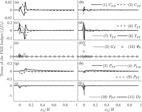
For steady state conditions, the budget of the spatially averaged TKE is given by: (5) $\begin{array}{rl}& \underset{\left(1\right):C_{TD}}{\underbrace{\frac{1}{2}\frac{\mathrm{\partial }}{\mathrm{\partial }{x}_j}({\phi }_{Vm}⟨{\phi }_T\overline{u_i^{\mathrm{\prime }}{u}_i^{\mathrm{\prime }}}⟩⟨{\overline{u}}_j⟩)}}\\ & =-\underset{\left(2\right):-P_{TT}}{\underbrace{{\phi }_{Vm}⟨{\phi }_T\overline{u_i^{\mathrm{\prime }}{u}_j^{\mathrm{\prime }}}⟩\frac{\mathrm{\partial }⟨{\overline{u}}_i⟩}{\mathrm{\partial }{x}_j}}}-\underset{\left(3\right):-P_{TF}}{\underbrace{{\phi }_{Vm}⟨{\phi }_T\overline{u_i^{\mathrm{\prime }}{u}_j^{\mathrm{\prime }}}\frac{\mathrm{\partial }{\tilde{\overline{u}}}_i}{\mathrm{\partial }{x}_j}⟩}}\\ & -\underset{\left(4\right):-T_{TF}}{\underbrace{\frac{1}{2}\frac{\mathrm{\partial }}{\mathrm{\partial }{x}_j}({\phi }_{Vm}⟨{\phi }_T\overline{u_i^{\mathrm{\prime }}{u}_i^{\mathrm{\prime }}}{\tilde{\overline{u}}}_j⟩)}}-\underset{\left(5\right):-T_{TT}}{\underbrace{\frac{1}{2}\frac{\mathrm{\partial }}{\mathrm{\partial }{x}_j}({\phi }_{Vm}⟨{\phi }_T\overline{u_i^{\mathrm{\prime }}{u}_i^{\mathrm{\prime }}{u}_j^{\mathrm{\prime }}}⟩)}}\\ & -\underset{\left(6\right):-T_{TP}}{\underbrace{\frac{1}{{\rho }_f}\frac{\mathrm{\partial }}{\mathrm{\partial }{x}_i}({\phi }_{Vm}⟨{\phi }_T\overline{u_i^{\mathrm{\prime }}{p}^{\mathrm{\prime }}}⟩)}}+\underset{\left(7\right):T_{TV}}{\underbrace{{\nu }_f\frac{\mathrm{\partial }}{\mathrm{\partial }{x}_j}\left({\phi }_{Vm}⟨{\phi }_T\overline{u_i^{\mathrm{\prime }}\frac{\mathrm{\partial }{u}_i^{\mathrm{\prime }}}{\mathrm{\partial }{x}_j}}⟩\right)}}\\ & +\underset{\left(8\right):P_{TP}}{\underbrace{\frac{{\phi }_{Vm}}{{\rho }_f}⟨{\phi }_T\overline{p^{\mathrm{\prime }}\frac{\mathrm{\partial }{u}_i^{\mathrm{\prime }}}{\mathrm{\partial }{x}_i}}⟩}}-\underset{\left(9\right):-D_T}{\underbrace{{\nu }_f{\phi }_{Vm}⟨{\phi }_T\overline{\frac{\mathrm{\partial }{u}_i^{\mathrm{\prime }}}{\mathrm{\partial }{x}_j}\frac{\mathrm{\partial }{u}_i^{\mathrm{\prime }}}{\mathrm{\partial }{x}_j}}⟩}}\\ & +\underset{\left(10\right):{\Phi }_T}{\underbrace{\frac{1}{{\rho }_f{V}_0}{\overline{{\int }_{S_{int}}{u}_i^{\mathrm{\prime }}p{n}_i\mathrm{d}S}}^s-\frac{1}{V_0}{\overline{{\int }_{S_{int}}{\nu }_f{u}_i^{\mathrm{\prime }}\frac{\mathrm{\partial }{u}_i}{\mathrm{\partial }{x}_j}{n}_j\mathrm{d}S}}^s}}\end{array}$(5) Terms 1, 4 and 5 in Eq. (5(5) $\begin{array}{rl}& \underset{\left(1\right):C_{TD}}{\underbrace{\frac{1}{2}\frac{\mathrm{\partial }}{\mathrm{\partial }{x}_j}({\phi }_{Vm}⟨{\phi }_T\overline{u_i^{\mathrm{\prime }}{u}_i^{\mathrm{\prime }}}⟩⟨{\overline{u}}_j⟩)}}\\ & =-\underset{\left(2\right):-P_{TT}}{\underbrace{{\phi }_{Vm}⟨{\phi }_T\overline{u_i^{\mathrm{\prime }}{u}_j^{\mathrm{\prime }}}⟩\frac{\mathrm{\partial }⟨{\overline{u}}_i⟩}{\mathrm{\partial }{x}_j}}}-\underset{\left(3\right):-P_{TF}}{\underbrace{{\phi }_{Vm}⟨{\phi }_T\overline{u_i^{\mathrm{\prime }}{u}_j^{\mathrm{\prime }}}\frac{\mathrm{\partial }{\tilde{\overline{u}}}_i}{\mathrm{\partial }{x}_j}⟩}}\\ & -\underset{\left(4\right):-T_{TF}}{\underbrace{\frac{1}{2}\frac{\mathrm{\partial }}{\mathrm{\partial }{x}_j}({\phi }_{Vm}⟨{\phi }_T\overline{u_i^{\mathrm{\prime }}{u}_i^{\mathrm{\prime }}}{\tilde{\overline{u}}}_j⟩)}}-\underset{\left(5\right):-T_{TT}}{\underbrace{\frac{1}{2}\frac{\mathrm{\partial }}{\mathrm{\partial }{x}_j}({\phi }_{Vm}⟨{\phi }_T\overline{u_i^{\mathrm{\prime }}{u}_i^{\mathrm{\prime }}{u}_j^{\mathrm{\prime }}}⟩)}}\\ & -\underset{\left(6\right):-T_{TP}}{\underbrace{\frac{1}{{\rho }_f}\frac{\mathrm{\partial }}{\mathrm{\partial }{x}_i}({\phi }_{Vm}⟨{\phi }_T\overline{u_i^{\mathrm{\prime }}{p}^{\mathrm{\prime }}}⟩)}}+\underset{\left(7\right):T_{TV}}{\underbrace{{\nu }_f\frac{\mathrm{\partial }}{\mathrm{\partial }{x}_j}\left({\phi }_{Vm}⟨{\phi }_T\overline{u_i^{\mathrm{\prime }}\frac{\mathrm{\partial }{u}_i^{\mathrm{\prime }}}{\mathrm{\partial }{x}_j}}⟩\right)}}\\ & +\underset{\left(8\right):P_{TP}}{\underbrace{\frac{{\phi }_{Vm}}{{\rho }_f}⟨{\phi }_T\overline{p^{\mathrm{\prime }}\frac{\mathrm{\partial }{u}_i^{\mathrm{\prime }}}{\mathrm{\partial }{x}_i}}⟩}}-\underset{\left(9\right):-D_T}{\underbrace{{\nu }_f{\phi }_{Vm}⟨{\phi }_T\overline{\frac{\mathrm{\partial }{u}_i^{\mathrm{\prime }}}{\mathrm{\partial }{x}_j}\frac{\mathrm{\partial }{u}_i^{\mathrm{\prime }}}{\mathrm{\partial }{x}_j}}⟩}}\\ & +\underset{\left(10\right):{\Phi }_T}{\underbrace{\frac{1}{{\rho }_f{V}_0}{\overline{{\int }_{S_{int}}{u}_i^{\mathrm{\prime }}p{n}_i\mathrm{d}S}}^s-\frac{1}{V_0}{\overline{{\int }_{S_{int}}{\nu }_f{u}_i^{\mathrm{\prime }}\frac{\mathrm{\partial }{u}_i}{\mathrm{\partial }{x}_j}{n}_j\mathrm{d}S}}^s}}\end{array}$(5) ) represent the convective transport of the turbulent energy by the double-mean, form-induced and turbulent velocities, respectively. Terms 2 and 3 reflect the energy exchange with the double-mean and form-induced velocity fields, respectively. Terms 6 and 7 are due to the pressure and viscous transport effects. Term 8 represents the inter-component energy transfer that is typically zero for fixed-bed flow conditions. This term is not considered to be zero for mobile-boundary flow conditions, when the spatial and temporal variation of ${\phi }_T$ may cause a non-zero mean strain rate $\mathrm{\partial }{\overline{u}}_i/\mathrm{\partial }{x}_i$ (Papadopoulos et al., 2019). The viscous dissipation of turbulent energy into heat is expressed by term 9, while term 10 reflects the exchange of energy between the turbulent field and the boundary motion due to the work of pressure and viscous stresses on the interfacial surface.

2.3. Background to the simulation scenarios

Vowinckel et al. (2017a, 2017b) provided background information on the simulation scenarios and the assessment of the double-averaged momentum balance for the same dataset as used here. Based on the selection criteria described in Section 2.2, the appropriate averaging time and volume have been selected. The averaging time $T_0$ was chosen to be equal to the total simulation time (starting after the initialization period) to enhance convergence for time-averaged quantities (first and second-order statistical moments). Regarding $T_0$, Vowinckel et al. (2017a) found that the sampling errors of the time-averaged velocities and Reynolds stresses reduce with increasing $T_0$ and become small for averaging times larger than $150H/U_b$. No time variations of the time-averaged fields are considered, as the flow rate through the averaging domain was kept constant to secure steady flow conditions in terms of time-averaged quantities. The selected averaging period ensured a clear separation between the mean and turbulent time scales. Two options are considered in the selection of the averaging volume: the “global' and “local” averaging domains, where spatial integration (Eq. 1(1) $\begin{array}{rl}⟨\overline{\theta }⟩& =\frac{1}{V_m}{\int }_{V_0}\frac{1}{T_f}{\int }_{T_0}\theta (x_i,t)\gamma (x_i,t)\mathrm{d}t\mathrm{d}V,\\ ⟨{\overline{\theta }}^s{⟩}^s& =\frac{1}{V_0}{\int }_{V_0}\frac{1}{T_0}{\int }_{T_0}\theta (x_i,t)\gamma (x_i,t)\mathrm{d}t\mathrm{d}V\end{array}$(1) ) is performed over the volumes $V_{0,1}=12H\times 6H\times \mathrm{\Delta }z$ and $V_{0,2}=12H\times 2D\times \mathrm{\Delta }z$, respectively, where $\mathrm{\Delta }z$ is the bed-normal cell size of the simulation grid. Note that the dimensions of the “global” averaging volume $V_{0,1}$ in the streamwise and spanwise directions coincide with the respective dimensions of the whole computational domain. The averaging operation over $V_{0,1}$ smooths flow heterogeneity in the streamwise and spanwise directions while fully resolving flow heterogeneity in the vertical direction, at least at scales larger than $\mathrm{\Delta }z$. Averaging over the “local” volume $V_{0,2}$ smooths streamwise heterogeneity, but resolves flow heterogeneity in the spanwise and bed-normal directions at scales larger than $2D$ and $\mathrm{\Delta }z$, respectively. Double-averaged variables obtained by employing the “global” and “local' averaging schemes are referred to here as “global” and “local” quantities, respectively. The detailed justification of the averaging time period $T_0$ and spatial averaging domains $V_{0,1}$ and $V_{0,2}$ is given in Vowinckel et al. (2017a). The following subsections summarize the key findings of Vowinckel et al. (2017a, 2017b) as the underpinning background for the current analysis.

Scenario HP: Instantaneous “snapshot” distributions of the bed particles are given in Vowinckel et al. (2017a, Fig. 3). In these snapshots, mobile particles were classified as moving particles or resting particles based on the ratio of particle to fluid velocity. Resting particles were accumulated within three streamwise zones of deposition with average spanwise spacing of $2H$. Clusters of resting particles formed in each zone with streamwise lengths of clusters varying from $12H$ at $x_2\approx (2-3.5)H$ (cluster 2) to $2H$ at $x_2\approx 0$ (cluster 1) and $x_2\approx 4H$ (cluster 3). The upstream part of cluster 1 was covered by moving particles, while cluster 3 was formed by irregularly distributed moving and resting particles. Similar observations can be made based on the distributions of space-averaged time porosity ${\phi }_T$ that are indicative of the average particle occupancy, rather than their instantaneous distribution. At points where $⟨{\phi }_T⟩>0.5$, mobile particles occupied these positions for less than half of the total averaging time. Thus, aggregations of mobile particles in such positions are considered as evolving ones, while aggregations of mobile particles with $⟨{\phi }_T⟩<0.5$ are more stable with time. The low values of global time porosity $⟨{\phi }_T⟩$ and streamwise velocity $⟨{\overline{u}}_1⟩$ in the zone $0\le x_3\le 0.1H$ suggest that HP tend to form clusters in this region. The spatial distribution of the local $⟨{\phi }_T⟩$ suggests the formation of a cluster (cluster 2) that is not frequently deformed by the flow at $1.5H\le x_2\le 2.5H$ where $⟨{\phi }_T⟩<0.5$, and two clusters: one (cluster 1) at $x_2=0$ where $0.6<⟨{\phi }_T⟩<0.7$, and one (cluster 3) migrating within the region $3.5H\le x_2<6H$ where $0.7<⟨{\phi }_T⟩<0.8$. As the time spent by mobile particles at the positions of clusters 1 and 3 is less than for cluster 2, clusters 1 and 3 are considered as “evolving” and cluster 2 as “more stable”. At $x_3=-D/2$, space porosity ${\phi }_{Vm}$ is close to 0 suggesting that particles are not moved from their place by the flow (as they are indeed fixed at position), while the increase of ${\phi }_{Vm}$ close to 1 at $x_3=-D$ and 0 shows the fluid covering the space in the gaps between fixed particles.

Scenario LP: The number of moving particles at a larger Shields number (LP) is significantly larger than scenario HP (Fig. 4 in Vowinckel et al., 2017a). The number of inter-particle collisions is consequently increased and the formation of small-scale particle aggregations with $0.5<⟨{\phi }_T⟩<0.9$ is observed for LP. The difference in bed-normal thickness of the particle mobility zone between the two scenarios is also noteworthy. In scenario HP the moving particles are typically below $x_3\approx 0.25H$, while moving particles in scenario LP spread up to the level $x_3\approx 0.5H$. Compared to the magnitude of the globally averaged time porosity $⟨{\phi }_T⟩$ for scenario HP, its lowest value in the layer $0<x_3<0.2H$ is higher for scenario LP. The distribution of the local average time porosity $⟨{\phi }_T⟩$ in the spanwise direction is more homogeneous compared to scenario HP and no particle aggregations can be seen due to more randomly distributed moving particles. Lower values of $⟨{\phi }_T⟩$ are noted approximately at $x_2\approx 0.5H$, 1.8H, $4H$ and 5.5H within the layer $0<x_3<0.1H$, suggesting that the time spend by the fluid at these points is shorter than in other regions within this layer. These local spanwise variations of time porosity indicate the development of small-scale clusters at these positions. As for scenario HP, the layer of fixed particles is accurately captured by the distribution of ${\phi }_{Vm}$.

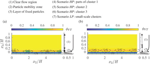
Figure 1 shows the distributions of local and global space-time porosity ${\phi }_{VT}={\phi }_{Vm}⟨{\phi }_T⟩$ and thus highlights key features of bed morphology for both scenarios. To allow the comparison between estimates from two scenarios as well as the comparison between distributions of local and global averages, each subfigure (i.e. Fig. 1a and b) consists of two plots. The plot on the left presents the spatial distribution of local ${\phi }_{VT}$ while the plot on the right shows the vertical distribution of global ${\phi }_{VT}$. For both scenarios, streamwise flow heterogeneity is stronger compared to spanwise and vertical directions, which is reflected in form-induced stresses, i.e. $⟨{\tilde{\overline{u}}}_1{\tilde{\overline{u}}}_1⟩\gg ⟨{\tilde{\overline{u}}}_2{\tilde{\overline{u}}}_2⟩\gg ⟨{\tilde{\overline{u}}}_3{\tilde{\overline{u}}}_3⟩$ (Fig. 6 in Vowinckel et al., 2017b). The effect of bed heterogeneity on the distributions of the form-induced stress components is most notable for the HP scenario. The data analysis in Vowinckel et al. (2017a, 2017b) show that form-induced stresses in mobile granular beds may contribute significantly to the total fluid stresses, and thus play considerable role in energy exchanges. Spatially averaged turbulent energy and primary shear stress are much stronger for scenario HP than LP, while the streamwise energy component dominates TKE (fig. 5 in Vowinckel et al., 2017b). The magnitude of momentum fluxes associated with the spatial correlations between time-porosity and time-averaged velocity (i.e. term IIB) is insignificant (thus its distributions were not presented).

Figure 1. Spatial distributions of the local (left-side plot in each subfigure) and global (right-side plot in each subfigure) space-time porosity ${\phi }_{VT}$ for scenarios HP (a) and LP (b), showing key features of bed morphology based on the distributions of ${\phi }_{VT}$

3. Results

Due to periodic boundary conditions along and across the flow in the simulations, the derivatives with respect to $x_1$ and $x_2$ in Eqs (3(3) $\begin{array}{rl}& \underset{\left(1\right):C_{DD}}{\underbrace{\frac{1}{2}\frac{\mathrm{\partial }}{\mathrm{\partial }{x}_j}({\phi }_{VT}⟨{\overline{u}}_i⟩⟨{\overline{u}}_i⟩⟨{\overline{u}}_j⟩)}}+\underset{\left(2\right):C_{DM}}{\underbrace{\frac{\mathrm{\partial }}{\mathrm{\partial }{x}_j}({\phi }_{Vm}⟨{\phi }_T{\tilde{\overline{u}}}_i⟩⟨{\overline{u}}_i⟩⟨{\overline{u}}_j⟩)}}\\ & =\underset{\left(3\right):G_D}{\underbrace{{\phi }_{VT}⟨{\overline{u}}_1⟩f_1}}-\underset{\left(4\right):-T_{DT}}{\underbrace{\frac{\mathrm{\partial }}{\mathrm{\partial }{x}_j}({\phi }_{Vm}⟨{\phi }_T\overline{u_i^{\mathrm{\prime }}{u}_j^{\mathrm{\prime }}}⟩⟨{\overline{u}}_i⟩)}}\\ & -\underset{\left(5\right):-T_{DF}}{\underbrace{\frac{\mathrm{\partial }}{\mathrm{\partial }{x}_j}({\phi }_{Vm}⟨{\phi }_T{\tilde{\overline{u}}}_i{\tilde{\overline{u}}}_j⟩⟨{\overline{u}}_i⟩)}}-\underset{\left(6\right):-T_{DM}}{\underbrace{\frac{1}{2}\frac{\mathrm{\partial }}{\mathrm{\partial }{x}_j}({\phi }_{Vm}⟨{\phi }_T{\tilde{\overline{u}}}_j⟩⟨{\overline{u}}_i⟩⟨{\overline{u}}_i⟩)}}\\ & -\underset{\left(7\right):-T_{DP}}{\underbrace{\frac{1}{{\rho }_f}\frac{\mathrm{\partial }}{\mathrm{\partial }{x}_i}({\phi }_{Vm}⟨{\phi }_T\overline{p}⟩⟨{\overline{u}}_i⟩)}}+\underset{\left(8\right):T_{DV}}{\underbrace{{\nu }_f\frac{\mathrm{\partial }}{\mathrm{\partial }{x}_j}({\phi }_{Vm}⟨{\phi }_T\overline{\frac{\mathrm{\partial }{u}_i}{\mathrm{\partial }{x}_j}}⟩⟨{\overline{u}}_i⟩)}}\\ & +\underset{\left(9\right):P_{DT}}{\underbrace{{\phi }_{Vm}⟨{\phi }_T\overline{u_i^{\mathrm{\prime }}{u}_j^{\mathrm{\prime }}}⟩\frac{\mathrm{\partial }⟨{\overline{u}}_i⟩}{\mathrm{\partial }{x}_j}}}+\underset{\left(10\right):P_{DF}}{\underbrace{{\phi }_{Vm}⟨{\phi }_T{\tilde{\overline{u}}}_i{\tilde{\overline{u}}}_j⟩\frac{\mathrm{\partial }⟨{\overline{u}}_i⟩}{\mathrm{\partial }{x}_j}}}\\ & +\underset{\left(11\right):P_{DM}}{\underbrace{{\phi }_{Vm}⟨{\phi }_T{\tilde{\overline{u}}}_i⟩⟨{\overline{u}}_j⟩\frac{\mathrm{\partial }⟨{\overline{u}}_i⟩}{\mathrm{\partial }{x}_j}}}\\ & +\underset{\left(12\right):P_{DP}}{\underbrace{\frac{{\phi }_{Vm}⟨{\phi }_T\overline{p}⟩}{{\rho }_f}\frac{\mathrm{\partial }⟨{\overline{u}}_i⟩}{\mathrm{\partial }{x}_i}}}-\underset{\left(13\right):-D_D}{\underbrace{{\nu }_f{\phi }_{Vm}⟨{\phi }_T\overline{\frac{\mathrm{\partial }{u}_i}{\mathrm{\partial }{x}_j}}⟩\frac{\mathrm{\partial }⟨{\overline{u}}_i⟩}{\mathrm{\partial }{x}_j}}}\\ & +\underset{\left(14\right):{\Phi }_D}{\underbrace{\frac{⟨{\overline{u}}_i⟩}{{\rho }_f{V}_0}{\overline{{\int }_{S_{int}}p{n}_i\mathrm{d}S}}^s-\frac{⟨{\overline{u}}_i⟩}{V_0}{\overline{{\int }_{S_{int}}{\nu }_f\frac{\mathrm{\partial }{u}_i}{\mathrm{\partial }{x}_j}{n}_j\mathrm{d}S}}^s}}\end{array}$(3) –5(5) $\begin{array}{rl}& \underset{\left(1\right):C_{TD}}{\underbrace{\frac{1}{2}\frac{\mathrm{\partial }}{\mathrm{\partial }{x}_j}({\phi }_{Vm}⟨{\phi }_T\overline{u_i^{\mathrm{\prime }}{u}_i^{\mathrm{\prime }}}⟩⟨{\overline{u}}_j⟩)}}\\ & =-\underset{\left(2\right):-P_{TT}}{\underbrace{{\phi }_{Vm}⟨{\phi }_T\overline{u_i^{\mathrm{\prime }}{u}_j^{\mathrm{\prime }}}⟩\frac{\mathrm{\partial }⟨{\overline{u}}_i⟩}{\mathrm{\partial }{x}_j}}}-\underset{\left(3\right):-P_{TF}}{\underbrace{{\phi }_{Vm}⟨{\phi }_T\overline{u_i^{\mathrm{\prime }}{u}_j^{\mathrm{\prime }}}\frac{\mathrm{\partial }{\tilde{\overline{u}}}_i}{\mathrm{\partial }{x}_j}⟩}}\\ & -\underset{\left(4\right):-T_{TF}}{\underbrace{\frac{1}{2}\frac{\mathrm{\partial }}{\mathrm{\partial }{x}_j}({\phi }_{Vm}⟨{\phi }_T\overline{u_i^{\mathrm{\prime }}{u}_i^{\mathrm{\prime }}}{\tilde{\overline{u}}}_j⟩)}}-\underset{\left(5\right):-T_{TT}}{\underbrace{\frac{1}{2}\frac{\mathrm{\partial }}{\mathrm{\partial }{x}_j}({\phi }_{Vm}⟨{\phi }_T\overline{u_i^{\mathrm{\prime }}{u}_i^{\mathrm{\prime }}{u}_j^{\mathrm{\prime }}}⟩)}}\\ & -\underset{\left(6\right):-T_{TP}}{\underbrace{\frac{1}{{\rho }_f}\frac{\mathrm{\partial }}{\mathrm{\partial }{x}_i}({\phi }_{Vm}⟨{\phi }_T\overline{u_i^{\mathrm{\prime }}{p}^{\mathrm{\prime }}}⟩)}}+\underset{\left(7\right):T_{TV}}{\underbrace{{\nu }_f\frac{\mathrm{\partial }}{\mathrm{\partial }{x}_j}\left({\phi }_{Vm}⟨{\phi }_T\overline{u_i^{\mathrm{\prime }}\frac{\mathrm{\partial }{u}_i^{\mathrm{\prime }}}{\mathrm{\partial }{x}_j}}⟩\right)}}\\ & +\underset{\left(8\right):P_{TP}}{\underbrace{\frac{{\phi }_{Vm}}{{\rho }_f}⟨{\phi }_T\overline{p^{\mathrm{\prime }}\frac{\mathrm{\partial }{u}_i^{\mathrm{\prime }}}{\mathrm{\partial }{x}_i}}⟩}}-\underset{\left(9\right):-D_T}{\underbrace{{\nu }_f{\phi }_{Vm}⟨{\phi }_T\overline{\frac{\mathrm{\partial }{u}_i^{\mathrm{\prime }}}{\mathrm{\partial }{x}_j}\frac{\mathrm{\partial }{u}_i^{\mathrm{\prime }}}{\mathrm{\partial }{x}_j}}⟩}}\\ & +\underset{\left(10\right):{\Phi }_T}{\underbrace{\frac{1}{{\rho }_f{V}_0}{\overline{{\int }_{S_{int}}{u}_i^{\mathrm{\prime }}p{n}_i\mathrm{d}S}}^s-\frac{1}{V_0}{\overline{{\int }_{S_{int}}{\nu }_f{u}_i^{\mathrm{\prime }}\frac{\mathrm{\partial }{u}_i}{\mathrm{\partial }{x}_j}{n}_j\mathrm{d}S}}^s}}\end{array}$(5) ) vanish when the global averaging scheme is applied. In the case of the local averaging scheme, only derivatives with respect to $x_1$ disappear for a similar reason. Pressure and viscous integrals could not be estimated directly due to limitations of the IBM method (Uhlmann, 2005). Instead, the interfacial terms in Eqs (3(3) $\begin{array}{rl}& \underset{\left(1\right):C_{DD}}{\underbrace{\frac{1}{2}\frac{\mathrm{\partial }}{\mathrm{\partial }{x}_j}({\phi }_{VT}⟨{\overline{u}}_i⟩⟨{\overline{u}}_i⟩⟨{\overline{u}}_j⟩)}}+\underset{\left(2\right):C_{DM}}{\underbrace{\frac{\mathrm{\partial }}{\mathrm{\partial }{x}_j}({\phi }_{Vm}⟨{\phi }_T{\tilde{\overline{u}}}_i⟩⟨{\overline{u}}_i⟩⟨{\overline{u}}_j⟩)}}\\ & =\underset{\left(3\right):G_D}{\underbrace{{\phi }_{VT}⟨{\overline{u}}_1⟩f_1}}-\underset{\left(4\right):-T_{DT}}{\underbrace{\frac{\mathrm{\partial }}{\mathrm{\partial }{x}_j}({\phi }_{Vm}⟨{\phi }_T\overline{u_i^{\mathrm{\prime }}{u}_j^{\mathrm{\prime }}}⟩⟨{\overline{u}}_i⟩)}}\\ & -\underset{\left(5\right):-T_{DF}}{\underbrace{\frac{\mathrm{\partial }}{\mathrm{\partial }{x}_j}({\phi }_{Vm}⟨{\phi }_T{\tilde{\overline{u}}}_i{\tilde{\overline{u}}}_j⟩⟨{\overline{u}}_i⟩)}}-\underset{\left(6\right):-T_{DM}}{\underbrace{\frac{1}{2}\frac{\mathrm{\partial }}{\mathrm{\partial }{x}_j}({\phi }_{Vm}⟨{\phi }_T{\tilde{\overline{u}}}_j⟩⟨{\overline{u}}_i⟩⟨{\overline{u}}_i⟩)}}\\ & -\underset{\left(7\right):-T_{DP}}{\underbrace{\frac{1}{{\rho }_f}\frac{\mathrm{\partial }}{\mathrm{\partial }{x}_i}({\phi }_{Vm}⟨{\phi }_T\overline{p}⟩⟨{\overline{u}}_i⟩)}}+\underset{\left(8\right):T_{DV}}{\underbrace{{\nu }_f\frac{\mathrm{\partial }}{\mathrm{\partial }{x}_j}({\phi }_{Vm}⟨{\phi }_T\overline{\frac{\mathrm{\partial }{u}_i}{\mathrm{\partial }{x}_j}}⟩⟨{\overline{u}}_i⟩)}}\\ & +\underset{\left(9\right):P_{DT}}{\underbrace{{\phi }_{Vm}⟨{\phi }_T\overline{u_i^{\mathrm{\prime }}{u}_j^{\mathrm{\prime }}}⟩\frac{\mathrm{\partial }⟨{\overline{u}}_i⟩}{\mathrm{\partial }{x}_j}}}+\underset{\left(10\right):P_{DF}}{\underbrace{{\phi }_{Vm}⟨{\phi }_T{\tilde{\overline{u}}}_i{\tilde{\overline{u}}}_j⟩\frac{\mathrm{\partial }⟨{\overline{u}}_i⟩}{\mathrm{\partial }{x}_j}}}\\ & +\underset{\left(11\right):P_{DM}}{\underbrace{{\phi }_{Vm}⟨{\phi }_T{\tilde{\overline{u}}}_i⟩⟨{\overline{u}}_j⟩\frac{\mathrm{\partial }⟨{\overline{u}}_i⟩}{\mathrm{\partial }{x}_j}}}\\ & +\underset{\left(12\right):P_{DP}}{\underbrace{\frac{{\phi }_{Vm}⟨{\phi }_T\overline{p}⟩}{{\rho }_f}\frac{\mathrm{\partial }⟨{\overline{u}}_i⟩}{\mathrm{\partial }{x}_i}}}-\underset{\left(13\right):-D_D}{\underbrace{{\nu }_f{\phi }_{Vm}⟨{\phi }_T\overline{\frac{\mathrm{\partial }{u}_i}{\mathrm{\partial }{x}_j}}⟩\frac{\mathrm{\partial }⟨{\overline{u}}_i⟩}{\mathrm{\partial }{x}_j}}}\\ & +\underset{\left(14\right):{\Phi }_D}{\underbrace{\frac{⟨{\overline{u}}_i⟩}{{\rho }_f{V}_0}{\overline{{\int }_{S_{int}}p{n}_i\mathrm{d}S}}^s-\frac{⟨{\overline{u}}_i⟩}{V_0}{\overline{{\int }_{S_{int}}{\nu }_f\frac{\mathrm{\partial }{u}_i}{\mathrm{\partial }{x}_j}{n}_j\mathrm{d}S}}^s}}\end{array}$(3) –5(5) $\begin{array}{rl}& \underset{\left(1\right):C_{TD}}{\underbrace{\frac{1}{2}\frac{\mathrm{\partial }}{\mathrm{\partial }{x}_j}({\phi }_{Vm}⟨{\phi }_T\overline{u_i^{\mathrm{\prime }}{u}_i^{\mathrm{\prime }}}⟩⟨{\overline{u}}_j⟩)}}\\ & =-\underset{\left(2\right):-P_{TT}}{\underbrace{{\phi }_{Vm}⟨{\phi }_T\overline{u_i^{\mathrm{\prime }}{u}_j^{\mathrm{\prime }}}⟩\frac{\mathrm{\partial }⟨{\overline{u}}_i⟩}{\mathrm{\partial }{x}_j}}}-\underset{\left(3\right):-P_{TF}}{\underbrace{{\phi }_{Vm}⟨{\phi }_T\overline{u_i^{\mathrm{\prime }}{u}_j^{\mathrm{\prime }}}\frac{\mathrm{\partial }{\tilde{\overline{u}}}_i}{\mathrm{\partial }{x}_j}⟩}}\\ & -\underset{\left(4\right):-T_{TF}}{\underbrace{\frac{1}{2}\frac{\mathrm{\partial }}{\mathrm{\partial }{x}_j}({\phi }_{Vm}⟨{\phi }_T\overline{u_i^{\mathrm{\prime }}{u}_i^{\mathrm{\prime }}}{\tilde{\overline{u}}}_j⟩)}}-\underset{\left(5\right):-T_{TT}}{\underbrace{\frac{1}{2}\frac{\mathrm{\partial }}{\mathrm{\partial }{x}_j}({\phi }_{Vm}⟨{\phi }_T\overline{u_i^{\mathrm{\prime }}{u}_i^{\mathrm{\prime }}{u}_j^{\mathrm{\prime }}}⟩)}}\\ & -\underset{\left(6\right):-T_{TP}}{\underbrace{\frac{1}{{\rho }_f}\frac{\mathrm{\partial }}{\mathrm{\partial }{x}_i}({\phi }_{Vm}⟨{\phi }_T\overline{u_i^{\mathrm{\prime }}{p}^{\mathrm{\prime }}}⟩)}}+\underset{\left(7\right):T_{TV}}{\underbrace{{\nu }_f\frac{\mathrm{\partial }}{\mathrm{\partial }{x}_j}\left({\phi }_{Vm}⟨{\phi }_T\overline{u_i^{\mathrm{\prime }}\frac{\mathrm{\partial }{u}_i^{\mathrm{\prime }}}{\mathrm{\partial }{x}_j}}⟩\right)}}\\ & +\underset{\left(8\right):P_{TP}}{\underbrace{\frac{{\phi }_{Vm}}{{\rho }_f}⟨{\phi }_T\overline{p^{\mathrm{\prime }}\frac{\mathrm{\partial }{u}_i^{\mathrm{\prime }}}{\mathrm{\partial }{x}_i}}⟩}}-\underset{\left(9\right):-D_T}{\underbrace{{\nu }_f{\phi }_{Vm}⟨{\phi }_T\overline{\frac{\mathrm{\partial }{u}_i^{\mathrm{\prime }}}{\mathrm{\partial }{x}_j}\frac{\mathrm{\partial }{u}_i^{\mathrm{\prime }}}{\mathrm{\partial }{x}_j}}⟩}}\\ & +\underset{\left(10\right):{\Phi }_T}{\underbrace{\frac{1}{{\rho }_f{V}_0}{\overline{{\int }_{S_{int}}{u}_i^{\mathrm{\prime }}p{n}_i\mathrm{d}S}}^s-\frac{1}{V_0}{\overline{{\int }_{S_{int}}{\nu }_f{u}_i^{\mathrm{\prime }}\frac{\mathrm{\partial }{u}_i}{\mathrm{\partial }{x}_j}{n}_j\mathrm{d}S}}^s}}\end{array}$(5) ) are computed as the out-of-balance quantities, assuming that the errors involved in the estimates of the other terms are small.

In the following sections, the global averaging scheme is used to identify large-scale mechanisms of energy transfers in the vertical direction, while the local scheme is used to study of energy transfer mechanisms in relation to the spanwise bed heterogeneity. In the plots shown in this section, the estimates of the terms of Eqs (3(3) $\begin{array}{rl}& \underset{\left(1\right):C_{DD}}{\underbrace{\frac{1}{2}\frac{\mathrm{\partial }}{\mathrm{\partial }{x}_j}({\phi }_{VT}⟨{\overline{u}}_i⟩⟨{\overline{u}}_i⟩⟨{\overline{u}}_j⟩)}}+\underset{\left(2\right):C_{DM}}{\underbrace{\frac{\mathrm{\partial }}{\mathrm{\partial }{x}_j}({\phi }_{Vm}⟨{\phi }_T{\tilde{\overline{u}}}_i⟩⟨{\overline{u}}_i⟩⟨{\overline{u}}_j⟩)}}\\ & =\underset{\left(3\right):G_D}{\underbrace{{\phi }_{VT}⟨{\overline{u}}_1⟩f_1}}-\underset{\left(4\right):-T_{DT}}{\underbrace{\frac{\mathrm{\partial }}{\mathrm{\partial }{x}_j}({\phi }_{Vm}⟨{\phi }_T\overline{u_i^{\mathrm{\prime }}{u}_j^{\mathrm{\prime }}}⟩⟨{\overline{u}}_i⟩)}}\\ & -\underset{\left(5\right):-T_{DF}}{\underbrace{\frac{\mathrm{\partial }}{\mathrm{\partial }{x}_j}({\phi }_{Vm}⟨{\phi }_T{\tilde{\overline{u}}}_i{\tilde{\overline{u}}}_j⟩⟨{\overline{u}}_i⟩)}}-\underset{\left(6\right):-T_{DM}}{\underbrace{\frac{1}{2}\frac{\mathrm{\partial }}{\mathrm{\partial }{x}_j}({\phi }_{Vm}⟨{\phi }_T{\tilde{\overline{u}}}_j⟩⟨{\overline{u}}_i⟩⟨{\overline{u}}_i⟩)}}\\ & -\underset{\left(7\right):-T_{DP}}{\underbrace{\frac{1}{{\rho }_f}\frac{\mathrm{\partial }}{\mathrm{\partial }{x}_i}({\phi }_{Vm}⟨{\phi }_T\overline{p}⟩⟨{\overline{u}}_i⟩)}}+\underset{\left(8\right):T_{DV}}{\underbrace{{\nu }_f\frac{\mathrm{\partial }}{\mathrm{\partial }{x}_j}({\phi }_{Vm}⟨{\phi }_T\overline{\frac{\mathrm{\partial }{u}_i}{\mathrm{\partial }{x}_j}}⟩⟨{\overline{u}}_i⟩)}}\\ & +\underset{\left(9\right):P_{DT}}{\underbrace{{\phi }_{Vm}⟨{\phi }_T\overline{u_i^{\mathrm{\prime }}{u}_j^{\mathrm{\prime }}}⟩\frac{\mathrm{\partial }⟨{\overline{u}}_i⟩}{\mathrm{\partial }{x}_j}}}+\underset{\left(10\right):P_{DF}}{\underbrace{{\phi }_{Vm}⟨{\phi }_T{\tilde{\overline{u}}}_i{\tilde{\overline{u}}}_j⟩\frac{\mathrm{\partial }⟨{\overline{u}}_i⟩}{\mathrm{\partial }{x}_j}}}\\ & +\underset{\left(11\right):P_{DM}}{\underbrace{{\phi }_{Vm}⟨{\phi }_T{\tilde{\overline{u}}}_i⟩⟨{\overline{u}}_j⟩\frac{\mathrm{\partial }⟨{\overline{u}}_i⟩}{\mathrm{\partial }{x}_j}}}\\ & +\underset{\left(12\right):P_{DP}}{\underbrace{\frac{{\phi }_{Vm}⟨{\phi }_T\overline{p}⟩}{{\rho }_f}\frac{\mathrm{\partial }⟨{\overline{u}}_i⟩}{\mathrm{\partial }{x}_i}}}-\underset{\left(13\right):-D_D}{\underbrace{{\nu }_f{\phi }_{Vm}⟨{\phi }_T\overline{\frac{\mathrm{\partial }{u}_i}{\mathrm{\partial }{x}_j}}⟩\frac{\mathrm{\partial }⟨{\overline{u}}_i⟩}{\mathrm{\partial }{x}_j}}}\\ & +\underset{\left(14\right):{\Phi }_D}{\underbrace{\frac{⟨{\overline{u}}_i⟩}{{\rho }_f{V}_0}{\overline{{\int }_{S_{int}}p{n}_i\mathrm{d}S}}^s-\frac{⟨{\overline{u}}_i⟩}{V_0}{\overline{{\int }_{S_{int}}{\nu }_f\frac{\mathrm{\partial }{u}_i}{\mathrm{\partial }{x}_j}{n}_j\mathrm{d}S}}^s}}\end{array}$(3) –5(5) $\begin{array}{rl}& \underset{\left(1\right):C_{TD}}{\underbrace{\frac{1}{2}\frac{\mathrm{\partial }}{\mathrm{\partial }{x}_j}({\phi }_{Vm}⟨{\phi }_T\overline{u_i^{\mathrm{\prime }}{u}_i^{\mathrm{\prime }}}⟩⟨{\overline{u}}_j⟩)}}\\ & =-\underset{\left(2\right):-P_{TT}}{\underbrace{{\phi }_{Vm}⟨{\phi }_T\overline{u_i^{\mathrm{\prime }}{u}_j^{\mathrm{\prime }}}⟩\frac{\mathrm{\partial }⟨{\overline{u}}_i⟩}{\mathrm{\partial }{x}_j}}}-\underset{\left(3\right):-P_{TF}}{\underbrace{{\phi }_{Vm}⟨{\phi }_T\overline{u_i^{\mathrm{\prime }}{u}_j^{\mathrm{\prime }}}\frac{\mathrm{\partial }{\tilde{\overline{u}}}_i}{\mathrm{\partial }{x}_j}⟩}}\\ & -\underset{\left(4\right):-T_{TF}}{\underbrace{\frac{1}{2}\frac{\mathrm{\partial }}{\mathrm{\partial }{x}_j}({\phi }_{Vm}⟨{\phi }_T\overline{u_i^{\mathrm{\prime }}{u}_i^{\mathrm{\prime }}}{\tilde{\overline{u}}}_j⟩)}}-\underset{\left(5\right):-T_{TT}}{\underbrace{\frac{1}{2}\frac{\mathrm{\partial }}{\mathrm{\partial }{x}_j}({\phi }_{Vm}⟨{\phi }_T\overline{u_i^{\mathrm{\prime }}{u}_i^{\mathrm{\prime }}{u}_j^{\mathrm{\prime }}}⟩)}}\\ & -\underset{\left(6\right):-T_{TP}}{\underbrace{\frac{1}{{\rho }_f}\frac{\mathrm{\partial }}{\mathrm{\partial }{x}_i}({\phi }_{Vm}⟨{\phi }_T\overline{u_i^{\mathrm{\prime }}{p}^{\mathrm{\prime }}}⟩)}}+\underset{\left(7\right):T_{TV}}{\underbrace{{\nu }_f\frac{\mathrm{\partial }}{\mathrm{\partial }{x}_j}\left({\phi }_{Vm}⟨{\phi }_T\overline{u_i^{\mathrm{\prime }}\frac{\mathrm{\partial }{u}_i^{\mathrm{\prime }}}{\mathrm{\partial }{x}_j}}⟩\right)}}\\ & +\underset{\left(8\right):P_{TP}}{\underbrace{\frac{{\phi }_{Vm}}{{\rho }_f}⟨{\phi }_T\overline{p^{\mathrm{\prime }}\frac{\mathrm{\partial }{u}_i^{\mathrm{\prime }}}{\mathrm{\partial }{x}_i}}⟩}}-\underset{\left(9\right):-D_T}{\underbrace{{\nu }_f{\phi }_{Vm}⟨{\phi }_T\overline{\frac{\mathrm{\partial }{u}_i^{\mathrm{\prime }}}{\mathrm{\partial }{x}_j}\frac{\mathrm{\partial }{u}_i^{\mathrm{\prime }}}{\mathrm{\partial }{x}_j}}⟩}}\\ & +\underset{\left(10\right):{\Phi }_T}{\underbrace{\frac{1}{{\rho }_f{V}_0}{\overline{{\int }_{S_{int}}{u}_i^{\mathrm{\prime }}p{n}_i\mathrm{d}S}}^s-\frac{1}{V_0}{\overline{{\int }_{S_{int}}{\nu }_f{u}_i^{\mathrm{\prime }}\frac{\mathrm{\partial }{u}_i}{\mathrm{\partial }{x}_j}{n}_j\mathrm{d}S}}^s}}\end{array}$(5) ) are normalized by $f_1{U}_b$, which is a measure of the external energy supply to the flow. Spatial coordinates are normalized by the flow depth H.

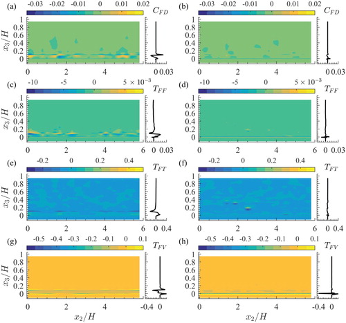
3.1. Budget of the double-mean energy

3.1.1. Relative significance of the terms in the DMKE budget: globally averaged quantities

The results for global averages in Eq. (3(3) $\begin{array}{rl}& \underset{\left(1\right):C_{DD}}{\underbrace{\frac{1}{2}\frac{\mathrm{\partial }}{\mathrm{\partial }{x}_j}({\phi }_{VT}⟨{\overline{u}}_i⟩⟨{\overline{u}}_i⟩⟨{\overline{u}}_j⟩)}}+\underset{\left(2\right):C_{DM}}{\underbrace{\frac{\mathrm{\partial }}{\mathrm{\partial }{x}_j}({\phi }_{Vm}⟨{\phi }_T{\tilde{\overline{u}}}_i⟩⟨{\overline{u}}_i⟩⟨{\overline{u}}_j⟩)}}\\ & =\underset{\left(3\right):G_D}{\underbrace{{\phi }_{VT}⟨{\overline{u}}_1⟩f_1}}-\underset{\left(4\right):-T_{DT}}{\underbrace{\frac{\mathrm{\partial }}{\mathrm{\partial }{x}_j}({\phi }_{Vm}⟨{\phi }_T\overline{u_i^{\mathrm{\prime }}{u}_j^{\mathrm{\prime }}}⟩⟨{\overline{u}}_i⟩)}}\\ & -\underset{\left(5\right):-T_{DF}}{\underbrace{\frac{\mathrm{\partial }}{\mathrm{\partial }{x}_j}({\phi }_{Vm}⟨{\phi }_T{\tilde{\overline{u}}}_i{\tilde{\overline{u}}}_j⟩⟨{\overline{u}}_i⟩)}}-\underset{\left(6\right):-T_{DM}}{\underbrace{\frac{1}{2}\frac{\mathrm{\partial }}{\mathrm{\partial }{x}_j}({\phi }_{Vm}⟨{\phi }_T{\tilde{\overline{u}}}_j⟩⟨{\overline{u}}_i⟩⟨{\overline{u}}_i⟩)}}\\ & -\underset{\left(7\right):-T_{DP}}{\underbrace{\frac{1}{{\rho }_f}\frac{\mathrm{\partial }}{\mathrm{\partial }{x}_i}({\phi }_{Vm}⟨{\phi }_T\overline{p}⟩⟨{\overline{u}}_i⟩)}}+\underset{\left(8\right):T_{DV}}{\underbrace{{\nu }_f\frac{\mathrm{\partial }}{\mathrm{\partial }{x}_j}({\phi }_{Vm}⟨{\phi }_T\overline{\frac{\mathrm{\partial }{u}_i}{\mathrm{\partial }{x}_j}}⟩⟨{\overline{u}}_i⟩)}}\\ & +\underset{\left(9\right):P_{DT}}{\underbrace{{\phi }_{Vm}⟨{\phi }_T\overline{u_i^{\mathrm{\prime }}{u}_j^{\mathrm{\prime }}}⟩\frac{\mathrm{\partial }⟨{\overline{u}}_i⟩}{\mathrm{\partial }{x}_j}}}+\underset{\left(10\right):P_{DF}}{\underbrace{{\phi }_{Vm}⟨{\phi }_T{\tilde{\overline{u}}}_i{\tilde{\overline{u}}}_j⟩\frac{\mathrm{\partial }⟨{\overline{u}}_i⟩}{\mathrm{\partial }{x}_j}}}\\ & +\underset{\left(11\right):P_{DM}}{\underbrace{{\phi }_{Vm}⟨{\phi }_T{\tilde{\overline{u}}}_i⟩⟨{\overline{u}}_j⟩\frac{\mathrm{\partial }⟨{\overline{u}}_i⟩}{\mathrm{\partial }{x}_j}}}\\ & +\underset{\left(12\right):P_{DP}}{\underbrace{\frac{{\phi }_{Vm}⟨{\phi }_T\overline{p}⟩}{{\rho }_f}\frac{\mathrm{\partial }⟨{\overline{u}}_i⟩}{\mathrm{\partial }{x}_i}}}-\underset{\left(13\right):-D_D}{\underbrace{{\nu }_f{\phi }_{Vm}⟨{\phi }_T\overline{\frac{\mathrm{\partial }{u}_i}{\mathrm{\partial }{x}_j}}⟩\frac{\mathrm{\partial }⟨{\overline{u}}_i⟩}{\mathrm{\partial }{x}_j}}}\\ & +\underset{\left(14\right):{\Phi }_D}{\underbrace{\frac{⟨{\overline{u}}_i⟩}{{\rho }_f{V}_0}{\overline{{\int }_{S_{int}}p{n}_i\mathrm{d}S}}^s-\frac{⟨{\overline{u}}_i⟩}{V_0}{\overline{{\int }_{S_{int}}{\nu }_f\frac{\mathrm{\partial }{u}_i}{\mathrm{\partial }{x}_j}{n}_j\mathrm{d}S}}^s}}\end{array}$(3) ) are illustrated in Fig. 2. Figure 2a and b show that among the left-hand side terms of Eq. (3(3) $\begin{array}{rl}& \underset{\left(1\right):C_{DD}}{\underbrace{\frac{1}{2}\frac{\mathrm{\partial }}{\mathrm{\partial }{x}_j}({\phi }_{VT}⟨{\overline{u}}_i⟩⟨{\overline{u}}_i⟩⟨{\overline{u}}_j⟩)}}+\underset{\left(2\right):C_{DM}}{\underbrace{\frac{\mathrm{\partial }}{\mathrm{\partial }{x}_j}({\phi }_{Vm}⟨{\phi }_T{\tilde{\overline{u}}}_i⟩⟨{\overline{u}}_i⟩⟨{\overline{u}}_j⟩)}}\\ & =\underset{\left(3\right):G_D}{\underbrace{{\phi }_{VT}⟨{\overline{u}}_1⟩f_1}}-\underset{\left(4\right):-T_{DT}}{\underbrace{\frac{\mathrm{\partial }}{\mathrm{\partial }{x}_j}({\phi }_{Vm}⟨{\phi }_T\overline{u_i^{\mathrm{\prime }}{u}_j^{\mathrm{\prime }}}⟩⟨{\overline{u}}_i⟩)}}\\ & -\underset{\left(5\right):-T_{DF}}{\underbrace{\frac{\mathrm{\partial }}{\mathrm{\partial }{x}_j}({\phi }_{Vm}⟨{\phi }_T{\tilde{\overline{u}}}_i{\tilde{\overline{u}}}_j⟩⟨{\overline{u}}_i⟩)}}-\underset{\left(6\right):-T_{DM}}{\underbrace{\frac{1}{2}\frac{\mathrm{\partial }}{\mathrm{\partial }{x}_j}({\phi }_{Vm}⟨{\phi }_T{\tilde{\overline{u}}}_j⟩⟨{\overline{u}}_i⟩⟨{\overline{u}}_i⟩)}}\\ & -\underset{\left(7\right):-T_{DP}}{\underbrace{\frac{1}{{\rho }_f}\frac{\mathrm{\partial }}{\mathrm{\partial }{x}_i}({\phi }_{Vm}⟨{\phi }_T\overline{p}⟩⟨{\overline{u}}_i⟩)}}+\underset{\left(8\right):T_{DV}}{\underbrace{{\nu }_f\frac{\mathrm{\partial }}{\mathrm{\partial }{x}_j}({\phi }_{Vm}⟨{\phi }_T\overline{\frac{\mathrm{\partial }{u}_i}{\mathrm{\partial }{x}_j}}⟩⟨{\overline{u}}_i⟩)}}\\ & +\underset{\left(9\right):P_{DT}}{\underbrace{{\phi }_{Vm}⟨{\phi }_T\overline{u_i^{\mathrm{\prime }}{u}_j^{\mathrm{\prime }}}⟩\frac{\mathrm{\partial }⟨{\overline{u}}_i⟩}{\mathrm{\partial }{x}_j}}}+\underset{\left(10\right):P_{DF}}{\underbrace{{\phi }_{Vm}⟨{\phi }_T{\tilde{\overline{u}}}_i{\tilde{\overline{u}}}_j⟩\frac{\mathrm{\partial }⟨{\overline{u}}_i⟩}{\mathrm{\partial }{x}_j}}}\\ & +\underset{\left(11\right):P_{DM}}{\underbrace{{\phi }_{Vm}⟨{\phi }_T{\tilde{\overline{u}}}_i⟩⟨{\overline{u}}_j⟩\frac{\mathrm{\partial }⟨{\overline{u}}_i⟩}{\mathrm{\partial }{x}_j}}}\\ & +\underset{\left(12\right):P_{DP}}{\underbrace{\frac{{\phi }_{Vm}⟨{\phi }_T\overline{p}⟩}{{\rho }_f}\frac{\mathrm{\partial }⟨{\overline{u}}_i⟩}{\mathrm{\partial }{x}_i}}}-\underset{\left(13\right):-D_D}{\underbrace{{\nu }_f{\phi }_{Vm}⟨{\phi }_T\overline{\frac{\mathrm{\partial }{u}_i}{\mathrm{\partial }{x}_j}}⟩\frac{\mathrm{\partial }⟨{\overline{u}}_i⟩}{\mathrm{\partial }{x}_j}}}\\ & +\underset{\left(14\right):{\Phi }_D}{\underbrace{\frac{⟨{\overline{u}}_i⟩}{{\rho }_f{V}_0}{\overline{{\int }_{S_{int}}p{n}_i\mathrm{d}S}}^s-\frac{⟨{\overline{u}}_i⟩}{V_0}{\overline{{\int }_{S_{int}}{\nu }_f\frac{\mathrm{\partial }{u}_i}{\mathrm{\partial }{x}_j}{n}_j\mathrm{d}S}}^s}}\end{array}$(3) ), DMKE convection $C_{DD}$ (term 1) is the most significant one for both scenarios, being particularly notable within the layer $0<x_3<0.4H$. However, compared to the rest of the transport terms given in the right-hand side of Eq. (3(3) $\begin{array}{rl}& \underset{\left(1\right):C_{DD}}{\underbrace{\frac{1}{2}\frac{\mathrm{\partial }}{\mathrm{\partial }{x}_j}({\phi }_{VT}⟨{\overline{u}}_i⟩⟨{\overline{u}}_i⟩⟨{\overline{u}}_j⟩)}}+\underset{\left(2\right):C_{DM}}{\underbrace{\frac{\mathrm{\partial }}{\mathrm{\partial }{x}_j}({\phi }_{Vm}⟨{\phi }_T{\tilde{\overline{u}}}_i⟩⟨{\overline{u}}_i⟩⟨{\overline{u}}_j⟩)}}\\ & =\underset{\left(3\right):G_D}{\underbrace{{\phi }_{VT}⟨{\overline{u}}_1⟩f_1}}-\underset{\left(4\right):-T_{DT}}{\underbrace{\frac{\mathrm{\partial }}{\mathrm{\partial }{x}_j}({\phi }_{Vm}⟨{\phi }_T\overline{u_i^{\mathrm{\prime }}{u}_j^{\mathrm{\prime }}}⟩⟨{\overline{u}}_i⟩)}}\\ & -\underset{\left(5\right):-T_{DF}}{\underbrace{\frac{\mathrm{\partial }}{\mathrm{\partial }{x}_j}({\phi }_{Vm}⟨{\phi }_T{\tilde{\overline{u}}}_i{\tilde{\overline{u}}}_j⟩⟨{\overline{u}}_i⟩)}}-\underset{\left(6\right):-T_{DM}}{\underbrace{\frac{1}{2}\frac{\mathrm{\partial }}{\mathrm{\partial }{x}_j}({\phi }_{Vm}⟨{\phi }_T{\tilde{\overline{u}}}_j⟩⟨{\overline{u}}_i⟩⟨{\overline{u}}_i⟩)}}\\ & -\underset{\left(7\right):-T_{DP}}{\underbrace{\frac{1}{{\rho }_f}\frac{\mathrm{\partial }}{\mathrm{\partial }{x}_i}({\phi }_{Vm}⟨{\phi }_T\overline{p}⟩⟨{\overline{u}}_i⟩)}}+\underset{\left(8\right):T_{DV}}{\underbrace{{\nu }_f\frac{\mathrm{\partial }}{\mathrm{\partial }{x}_j}({\phi }_{Vm}⟨{\phi }_T\overline{\frac{\mathrm{\partial }{u}_i}{\mathrm{\partial }{x}_j}}⟩⟨{\overline{u}}_i⟩)}}\\ & +\underset{\left(9\right):P_{DT}}{\underbrace{{\phi }_{Vm}⟨{\phi }_T\overline{u_i^{\mathrm{\prime }}{u}_j^{\mathrm{\prime }}}⟩\frac{\mathrm{\partial }⟨{\overline{u}}_i⟩}{\mathrm{\partial }{x}_j}}}+\underset{\left(10\right):P_{DF}}{\underbrace{{\phi }_{Vm}⟨{\phi }_T{\tilde{\overline{u}}}_i{\tilde{\overline{u}}}_j⟩\frac{\mathrm{\partial }⟨{\overline{u}}_i⟩}{\mathrm{\partial }{x}_j}}}\\ & +\underset{\left(11\right):P_{DM}}{\underbrace{{\phi }_{Vm}⟨{\phi }_T{\tilde{\overline{u}}}_i⟩⟨{\overline{u}}_j⟩\frac{\mathrm{\partial }⟨{\overline{u}}_i⟩}{\mathrm{\partial }{x}_j}}}\\ & +\underset{\left(12\right):P_{DP}}{\underbrace{\frac{{\phi }_{Vm}⟨{\phi }_T\overline{p}⟩}{{\rho }_f}\frac{\mathrm{\partial }⟨{\overline{u}}_i⟩}{\mathrm{\partial }{x}_i}}}-\underset{\left(13\right):-D_D}{\underbrace{{\nu }_f{\phi }_{Vm}⟨{\phi }_T\overline{\frac{\mathrm{\partial }{u}_i}{\mathrm{\partial }{x}_j}}⟩\frac{\mathrm{\partial }⟨{\overline{u}}_i⟩}{\mathrm{\partial }{x}_j}}}\\ & +\underset{\left(14\right):{\Phi }_D}{\underbrace{\frac{⟨{\overline{u}}_i⟩}{{\rho }_f{V}_0}{\overline{{\int }_{S_{int}}p{n}_i\mathrm{d}S}}^s-\frac{⟨{\overline{u}}_i⟩}{V_0}{\overline{{\int }_{S_{int}}{\nu }_f\frac{\mathrm{\partial }{u}_i}{\mathrm{\partial }{x}_j}{n}_j\mathrm{d}S}}^s}}\end{array}$(3) ), DMKE convection (term 1) is considerably lower. Energy transport is controlled by the work of the turbulent $T_{DT}$ (term 4) and viscous stresses $T_{DV}$ (term 8), particularly by their parts associated with the dominant streamwise energy components (Fig. 2c, e and d, f). The relative significance of the energy conversion terms is similar for both scenarios. The work of the form-induced stresses $P_{DF}$ (term 10) and the stresses associated with the porosity-correlation $P_{DM}$ (term 11) on the double-mean strain-rate are insignificant compared to the external energy supply $G_D$ (term 3), the conversion to turbulent energy $P_{DT}$ (term 9), dissipation to heat $D_D$ (term 13), and the interfacial exchange ${\Phi }_D$ (term 14).

Figure 2. Vertical distributions of the terms of the globally averaged DMKE balance of Eq. (3(3) $\begin{array}{rl}& \underset{\left(1\right):C_{DD}}{\underbrace{\frac{1}{2}\frac{\mathrm{\partial }}{\mathrm{\partial }{x}_j}({\phi }_{VT}⟨{\overline{u}}_i⟩⟨{\overline{u}}_i⟩⟨{\overline{u}}_j⟩)}}+\underset{\left(2\right):C_{DM}}{\underbrace{\frac{\mathrm{\partial }}{\mathrm{\partial }{x}_j}({\phi }_{Vm}⟨{\phi }_T{\tilde{\overline{u}}}_i⟩⟨{\overline{u}}_i⟩⟨{\overline{u}}_j⟩)}}\\ & =\underset{\left(3\right):G_D}{\underbrace{{\phi }_{VT}⟨{\overline{u}}_1⟩f_1}}-\underset{\left(4\right):-T_{DT}}{\underbrace{\frac{\mathrm{\partial }}{\mathrm{\partial }{x}_j}({\phi }_{Vm}⟨{\phi }_T\overline{u_i^{\mathrm{\prime }}{u}_j^{\mathrm{\prime }}}⟩⟨{\overline{u}}_i⟩)}}\\ & -\underset{\left(5\right):-T_{DF}}{\underbrace{\frac{\mathrm{\partial }}{\mathrm{\partial }{x}_j}({\phi }_{Vm}⟨{\phi }_T{\tilde{\overline{u}}}_i{\tilde{\overline{u}}}_j⟩⟨{\overline{u}}_i⟩)}}-\underset{\left(6\right):-T_{DM}}{\underbrace{\frac{1}{2}\frac{\mathrm{\partial }}{\mathrm{\partial }{x}_j}({\phi }_{Vm}⟨{\phi }_T{\tilde{\overline{u}}}_j⟩⟨{\overline{u}}_i⟩⟨{\overline{u}}_i⟩)}}\\ & -\underset{\left(7\right):-T_{DP}}{\underbrace{\frac{1}{{\rho }_f}\frac{\mathrm{\partial }}{\mathrm{\partial }{x}_i}({\phi }_{Vm}⟨{\phi }_T\overline{p}⟩⟨{\overline{u}}_i⟩)}}+\underset{\left(8\right):T_{DV}}{\underbrace{{\nu }_f\frac{\mathrm{\partial }}{\mathrm{\partial }{x}_j}({\phi }_{Vm}⟨{\phi }_T\overline{\frac{\mathrm{\partial }{u}_i}{\mathrm{\partial }{x}_j}}⟩⟨{\overline{u}}_i⟩)}}\\ & +\underset{\left(9\right):P_{DT}}{\underbrace{{\phi }_{Vm}⟨{\phi }_T\overline{u_i^{\mathrm{\prime }}{u}_j^{\mathrm{\prime }}}⟩\frac{\mathrm{\partial }⟨{\overline{u}}_i⟩}{\mathrm{\partial }{x}_j}}}+\underset{\left(10\right):P_{DF}}{\underbrace{{\phi }_{Vm}⟨{\phi }_T{\tilde{\overline{u}}}_i{\tilde{\overline{u}}}_j⟩\frac{\mathrm{\partial }⟨{\overline{u}}_i⟩}{\mathrm{\partial }{x}_j}}}\\ & +\underset{\left(11\right):P_{DM}}{\underbrace{{\phi }_{Vm}⟨{\phi }_T{\tilde{\overline{u}}}_i⟩⟨{\overline{u}}_j⟩\frac{\mathrm{\partial }⟨{\overline{u}}_i⟩}{\mathrm{\partial }{x}_j}}}\\ & +\underset{\left(12\right):P_{DP}}{\underbrace{\frac{{\phi }_{Vm}⟨{\phi }_T\overline{p}⟩}{{\rho }_f}\frac{\mathrm{\partial }⟨{\overline{u}}_i⟩}{\mathrm{\partial }{x}_i}}}-\underset{\left(13\right):-D_D}{\underbrace{{\nu }_f{\phi }_{Vm}⟨{\phi }_T\overline{\frac{\mathrm{\partial }{u}_i}{\mathrm{\partial }{x}_j}}⟩\frac{\mathrm{\partial }⟨{\overline{u}}_i⟩}{\mathrm{\partial }{x}_j}}}\\ & +\underset{\left(14\right):{\Phi }_D}{\underbrace{\frac{⟨{\overline{u}}_i⟩}{{\rho }_f{V}_0}{\overline{{\int }_{S_{int}}p{n}_i\mathrm{d}S}}^s-\frac{⟨{\overline{u}}_i⟩}{V_0}{\overline{{\int }_{S_{int}}{\nu }_f\frac{\mathrm{\partial }{u}_i}{\mathrm{\partial }{x}_j}{n}_j\mathrm{d}S}}^s}}\end{array}$(3) ): DMKE mean convection $C_{DD}$ (term 1) and velocity-time porosity correlation $C_{DM}$ (term 2) for scenarios HP (a) and LP (b); turbulent $T_{DT}$ (term 4), form-induced $T_{DF}$ (term 5) and velocity-time porosity transport $T_{DM}$ (term 6) of DMKE for scenarios HP (c) and LP (d); pressure $T_{DP}$ (term 7) and viscous transport $T_{DV}$ of DMKE (term 8) for scenarios HP (e) and LP (f); the energy supply $G_D$ (term 3), pressure work against bulk strain rate $P_{DP}$ (term 12), viscous dissipation to heat $D_D$ (term 13), and the interfacial energy exchange ${\Phi }_D$ (term 14) for scenarios HP (g) and LP (h); the energy exchange with the TKE balance $P_{DT}$ (term 9) and FKE balance $P_{DF}$ (term 10), $P_{DM}$ (term 11) for scenarios HP (i) and LP (j). The shown term values are normalized on $f_1{U}_b$

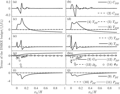
Kinetic energy is supplied to the double-mean velocity field from the work $G_D$ of the volume force $f_1$ (term 3; Fig. 2g and h). The external energy supply increases with distance from the bed, reflecting the distribution of the double-mean velocity and time-space porosity ${\phi }_{VT}$. The mean energy transport due to turbulent stresses $T_{DT}$ (term 4 in Eq. 3(3) $\begin{array}{rl}& \underset{\left(1\right):C_{DD}}{\underbrace{\frac{1}{2}\frac{\mathrm{\partial }}{\mathrm{\partial }{x}_j}({\phi }_{VT}⟨{\overline{u}}_i⟩⟨{\overline{u}}_i⟩⟨{\overline{u}}_j⟩)}}+\underset{\left(2\right):C_{DM}}{\underbrace{\frac{\mathrm{\partial }}{\mathrm{\partial }{x}_j}({\phi }_{Vm}⟨{\phi }_T{\tilde{\overline{u}}}_i⟩⟨{\overline{u}}_i⟩⟨{\overline{u}}_j⟩)}}\\ & =\underset{\left(3\right):G_D}{\underbrace{{\phi }_{VT}⟨{\overline{u}}_1⟩f_1}}-\underset{\left(4\right):-T_{DT}}{\underbrace{\frac{\mathrm{\partial }}{\mathrm{\partial }{x}_j}({\phi }_{Vm}⟨{\phi }_T\overline{u_i^{\mathrm{\prime }}{u}_j^{\mathrm{\prime }}}⟩⟨{\overline{u}}_i⟩)}}\\ & -\underset{\left(5\right):-T_{DF}}{\underbrace{\frac{\mathrm{\partial }}{\mathrm{\partial }{x}_j}({\phi }_{Vm}⟨{\phi }_T{\tilde{\overline{u}}}_i{\tilde{\overline{u}}}_j⟩⟨{\overline{u}}_i⟩)}}-\underset{\left(6\right):-T_{DM}}{\underbrace{\frac{1}{2}\frac{\mathrm{\partial }}{\mathrm{\partial }{x}_j}({\phi }_{Vm}⟨{\phi }_T{\tilde{\overline{u}}}_j⟩⟨{\overline{u}}_i⟩⟨{\overline{u}}_i⟩)}}\\ & -\underset{\left(7\right):-T_{DP}}{\underbrace{\frac{1}{{\rho }_f}\frac{\mathrm{\partial }}{\mathrm{\partial }{x}_i}({\phi }_{Vm}⟨{\phi }_T\overline{p}⟩⟨{\overline{u}}_i⟩)}}+\underset{\left(8\right):T_{DV}}{\underbrace{{\nu }_f\frac{\mathrm{\partial }}{\mathrm{\partial }{x}_j}({\phi }_{Vm}⟨{\phi }_T\overline{\frac{\mathrm{\partial }{u}_i}{\mathrm{\partial }{x}_j}}⟩⟨{\overline{u}}_i⟩)}}\\ & +\underset{\left(9\right):P_{DT}}{\underbrace{{\phi }_{Vm}⟨{\phi }_T\overline{u_i^{\mathrm{\prime }}{u}_j^{\mathrm{\prime }}}⟩\frac{\mathrm{\partial }⟨{\overline{u}}_i⟩}{\mathrm{\partial }{x}_j}}}+\underset{\left(10\right):P_{DF}}{\underbrace{{\phi }_{Vm}⟨{\phi }_T{\tilde{\overline{u}}}_i{\tilde{\overline{u}}}_j⟩\frac{\mathrm{\partial }⟨{\overline{u}}_i⟩}{\mathrm{\partial }{x}_j}}}\\ & +\underset{\left(11\right):P_{DM}}{\underbrace{{\phi }_{Vm}⟨{\phi }_T{\tilde{\overline{u}}}_i⟩⟨{\overline{u}}_j⟩\frac{\mathrm{\partial }⟨{\overline{u}}_i⟩}{\mathrm{\partial }{x}_j}}}\\ & +\underset{\left(12\right):P_{DP}}{\underbrace{\frac{{\phi }_{Vm}⟨{\phi }_T\overline{p}⟩}{{\rho }_f}\frac{\mathrm{\partial }⟨{\overline{u}}_i⟩}{\mathrm{\partial }{x}_i}}}-\underset{\left(13\right):-D_D}{\underbrace{{\nu }_f{\phi }_{Vm}⟨{\phi }_T\overline{\frac{\mathrm{\partial }{u}_i}{\mathrm{\partial }{x}_j}}⟩\frac{\mathrm{\partial }⟨{\overline{u}}_i⟩}{\mathrm{\partial }{x}_j}}}\\ & +\underset{\left(14\right):{\Phi }_D}{\underbrace{\frac{⟨{\overline{u}}_i⟩}{{\rho }_f{V}_0}{\overline{{\int }_{S_{int}}p{n}_i\mathrm{d}S}}^s-\frac{⟨{\overline{u}}_i⟩}{V_0}{\overline{{\int }_{S_{int}}{\nu }_f\frac{\mathrm{\partial }{u}_i}{\mathrm{\partial }{x}_j}{n}_j\mathrm{d}S}}^s}}\end{array}$(3) , Fig. 2c and d) is directed from upper to lower flow regions, with the energy loss above $x_3\approx 0.29H$ and $x_3\approx 0.32H$ for scenarios HP and LP, respectively, and the mean energy gain below these levels. The vertical profiles of $T_{DT}$ exhibit peaks at $x_3\approx 0.1H-0.15H$, consistent with the locations of the peaks of the primary shear Reynolds stress. As the Reynolds stresses become weaker downwards from the peak, the magnitude of term 4 reduces towards $x_3\approx 0$, where it vanishes. The work rate $P_{DT}$ of the Reynolds stresses against the double-mean strain rate (term 9) removes energy from the mean field in the layer $0<x_3<0.85H$, for both scenarios (Fig. 2i and j). This energy removal from the double-mean flow increases with decreasing distance from the bed, peaking at the level $x_3\approx 0.1H-0.15H$ for both scenarios. Below this level, the energy removed due to term 9 decreases down to 0 at $x_3\approx 0$. The work $T_{DV}$ of viscous stresses (term 8) transfers energy to thin layers at the levels $x_3=0$ and $x_3\approx 0.18H$ from thin regions just above these two layers, reflecting locations of flow–sediment interfaces: the top of the fixed particles' layer is at $x_3=0$ and the top level of the particle mobility zone is close to $x_3\approx 0.18H$ (Fig. 2e and f). The work $D_D$ of viscous stresses against the double-mean strain-rate converts the mean kinetic energy to heat (term 13) within thin layers at $x_3\approx 0.02H$ and $x_3\approx 0.1H$ (Fig. 2g and h). Due to the work ${\Phi }_D$ of pressure drag and viscous drag (term 14), the energy is supplied from the mean flow to particle motion (Fig. 2g and h). This energy conversion happens within the layers $0\le x_3\le 0.15H$ for scenario HP and $0\le x_3\le 0.25H$ for scenario LP. It should be noted that the relative time of exposure of fixed particles to the moving fluid for scenario LP is higher compared to scenario HP, leading to the enhanced viscous and pressure effects as well as the increased interfacial energy exchange noted at $x_3=0$ for scenario LP. The effect of pressure transport, that is negligible for scenario HP, becomes noticeable for scenario LP, although it is still weaker than turbulent and viscous transport. Effects of pressure work $P_{DP}$ on the double-mean strain rate (term 12; Fig. 2g and f) is negligible for both scenarios. Viscous transport $T_{DV}$ (term 8; Fig. 2e and f) transfers energy from a thin layer at $x_3\approx 0.02H-0.04H$ and the region $0.1H<x_3<0.3H$ to layers at $x_3\approx 0$ and $x_3\approx 0.08H$, for both scenarios.

3.1.2. Spatial variability of the terms in the DMKE budget: locally averaged quantities

The spatial distributions of the local estimates of the most significant terms 1, 3, 4, 8, 9 and 13 in Eq. (3(3) $\begin{array}{rl}& \underset{\left(1\right):C_{DD}}{\underbrace{\frac{1}{2}\frac{\mathrm{\partial }}{\mathrm{\partial }{x}_j}({\phi }_{VT}⟨{\overline{u}}_i⟩⟨{\overline{u}}_i⟩⟨{\overline{u}}_j⟩)}}+\underset{\left(2\right):C_{DM}}{\underbrace{\frac{\mathrm{\partial }}{\mathrm{\partial }{x}_j}({\phi }_{Vm}⟨{\phi }_T{\tilde{\overline{u}}}_i⟩⟨{\overline{u}}_i⟩⟨{\overline{u}}_j⟩)}}\\ & =\underset{\left(3\right):G_D}{\underbrace{{\phi }_{VT}⟨{\overline{u}}_1⟩f_1}}-\underset{\left(4\right):-T_{DT}}{\underbrace{\frac{\mathrm{\partial }}{\mathrm{\partial }{x}_j}({\phi }_{Vm}⟨{\phi }_T\overline{u_i^{\mathrm{\prime }}{u}_j^{\mathrm{\prime }}}⟩⟨{\overline{u}}_i⟩)}}\\ & -\underset{\left(5\right):-T_{DF}}{\underbrace{\frac{\mathrm{\partial }}{\mathrm{\partial }{x}_j}({\phi }_{Vm}⟨{\phi }_T{\tilde{\overline{u}}}_i{\tilde{\overline{u}}}_j⟩⟨{\overline{u}}_i⟩)}}-\underset{\left(6\right):-T_{DM}}{\underbrace{\frac{1}{2}\frac{\mathrm{\partial }}{\mathrm{\partial }{x}_j}({\phi }_{Vm}⟨{\phi }_T{\tilde{\overline{u}}}_j⟩⟨{\overline{u}}_i⟩⟨{\overline{u}}_i⟩)}}\\ & -\underset{\left(7\right):-T_{DP}}{\underbrace{\frac{1}{{\rho }_f}\frac{\mathrm{\partial }}{\mathrm{\partial }{x}_i}({\phi }_{Vm}⟨{\phi }_T\overline{p}⟩⟨{\overline{u}}_i⟩)}}+\underset{\left(8\right):T_{DV}}{\underbrace{{\nu }_f\frac{\mathrm{\partial }}{\mathrm{\partial }{x}_j}({\phi }_{Vm}⟨{\phi }_T\overline{\frac{\mathrm{\partial }{u}_i}{\mathrm{\partial }{x}_j}}⟩⟨{\overline{u}}_i⟩)}}\\ & +\underset{\left(9\right):P_{DT}}{\underbrace{{\phi }_{Vm}⟨{\phi }_T\overline{u_i^{\mathrm{\prime }}{u}_j^{\mathrm{\prime }}}⟩\frac{\mathrm{\partial }⟨{\overline{u}}_i⟩}{\mathrm{\partial }{x}_j}}}+\underset{\left(10\right):P_{DF}}{\underbrace{{\phi }_{Vm}⟨{\phi }_T{\tilde{\overline{u}}}_i{\tilde{\overline{u}}}_j⟩\frac{\mathrm{\partial }⟨{\overline{u}}_i⟩}{\mathrm{\partial }{x}_j}}}\\ & +\underset{\left(11\right):P_{DM}}{\underbrace{{\phi }_{Vm}⟨{\phi }_T{\tilde{\overline{u}}}_i⟩⟨{\overline{u}}_j⟩\frac{\mathrm{\partial }⟨{\overline{u}}_i⟩}{\mathrm{\partial }{x}_j}}}\\ & +\underset{\left(12\right):P_{DP}}{\underbrace{\frac{{\phi }_{Vm}⟨{\phi }_T\overline{p}⟩}{{\rho }_f}\frac{\mathrm{\partial }⟨{\overline{u}}_i⟩}{\mathrm{\partial }{x}_i}}}-\underset{\left(13\right):-D_D}{\underbrace{{\nu }_f{\phi }_{Vm}⟨{\phi }_T\overline{\frac{\mathrm{\partial }{u}_i}{\mathrm{\partial }{x}_j}}⟩\frac{\mathrm{\partial }⟨{\overline{u}}_i⟩}{\mathrm{\partial }{x}_j}}}\\ & +\underset{\left(14\right):{\Phi }_D}{\underbrace{\frac{⟨{\overline{u}}_i⟩}{{\rho }_f{V}_0}{\overline{{\int }_{S_{int}}p{n}_i\mathrm{d}S}}^s-\frac{⟨{\overline{u}}_i⟩}{V_0}{\overline{{\int }_{S_{int}}{\nu }_f\frac{\mathrm{\partial }{u}_i}{\mathrm{\partial }{x}_j}{n}_j\mathrm{d}S}}^s}}\end{array}$(3) ) are presented in Figs 3 and 4 to assess their spanwise and vertical heterogeneity. The distributions given in Figs 3 and 4 are organized as Fig. 1 is. Hence, the first two columns contain plots of local and global double-averaged quantities, respectively, for case HP, while the third and fourth columns have plots of local and global quantities for the LP case.

Figure 3. Spatial distributions of the energy converting terms of the DMKE balance of Eq. (3(3) $\begin{array}{rl}& \underset{\left(1\right):C_{DD}}{\underbrace{\frac{1}{2}\frac{\mathrm{\partial }}{\mathrm{\partial }{x}_j}({\phi }_{VT}⟨{\overline{u}}_i⟩⟨{\overline{u}}_i⟩⟨{\overline{u}}_j⟩)}}+\underset{\left(2\right):C_{DM}}{\underbrace{\frac{\mathrm{\partial }}{\mathrm{\partial }{x}_j}({\phi }_{Vm}⟨{\phi }_T{\tilde{\overline{u}}}_i⟩⟨{\overline{u}}_i⟩⟨{\overline{u}}_j⟩)}}\\ & =\underset{\left(3\right):G_D}{\underbrace{{\phi }_{VT}⟨{\overline{u}}_1⟩f_1}}-\underset{\left(4\right):-T_{DT}}{\underbrace{\frac{\mathrm{\partial }}{\mathrm{\partial }{x}_j}({\phi }_{Vm}⟨{\phi }_T\overline{u_i^{\mathrm{\prime }}{u}_j^{\mathrm{\prime }}}⟩⟨{\overline{u}}_i⟩)}}\\ & -\underset{\left(5\right):-T_{DF}}{\underbrace{\frac{\mathrm{\partial }}{\mathrm{\partial }{x}_j}({\phi }_{Vm}⟨{\phi }_T{\tilde{\overline{u}}}_i{\tilde{\overline{u}}}_j⟩⟨{\overline{u}}_i⟩)}}-\underset{\left(6\right):-T_{DM}}{\underbrace{\frac{1}{2}\frac{\mathrm{\partial }}{\mathrm{\partial }{x}_j}({\phi }_{Vm}⟨{\phi }_T{\tilde{\overline{u}}}_j⟩⟨{\overline{u}}_i⟩⟨{\overline{u}}_i⟩)}}\\ & -\underset{\left(7\right):-T_{DP}}{\underbrace{\frac{1}{{\rho }_f}\frac{\mathrm{\partial }}{\mathrm{\partial }{x}_i}({\phi }_{Vm}⟨{\phi }_T\overline{p}⟩⟨{\overline{u}}_i⟩)}}+\underset{\left(8\right):T_{DV}}{\underbrace{{\nu }_f\frac{\mathrm{\partial }}{\mathrm{\partial }{x}_j}({\phi }_{Vm}⟨{\phi }_T\overline{\frac{\mathrm{\partial }{u}_i}{\mathrm{\partial }{x}_j}}⟩⟨{\overline{u}}_i⟩)}}\\ & +\underset{\left(9\right):P_{DT}}{\underbrace{{\phi }_{Vm}⟨{\phi }_T\overline{u_i^{\mathrm{\prime }}{u}_j^{\mathrm{\prime }}}⟩\frac{\mathrm{\partial }⟨{\overline{u}}_i⟩}{\mathrm{\partial }{x}_j}}}+\underset{\left(10\right):P_{DF}}{\underbrace{{\phi }_{Vm}⟨{\phi }_T{\tilde{\overline{u}}}_i{\tilde{\overline{u}}}_j⟩\frac{\mathrm{\partial }⟨{\overline{u}}_i⟩}{\mathrm{\partial }{x}_j}}}\\ & +\underset{\left(11\right):P_{DM}}{\underbrace{{\phi }_{Vm}⟨{\phi }_T{\tilde{\overline{u}}}_i⟩⟨{\overline{u}}_j⟩\frac{\mathrm{\partial }⟨{\overline{u}}_i⟩}{\mathrm{\partial }{x}_j}}}\\ & +\underset{\left(12\right):P_{DP}}{\underbrace{\frac{{\phi }_{Vm}⟨{\phi }_T\overline{p}⟩}{{\rho }_f}\frac{\mathrm{\partial }⟨{\overline{u}}_i⟩}{\mathrm{\partial }{x}_i}}}-\underset{\left(13\right):-D_D}{\underbrace{{\nu }_f{\phi }_{Vm}⟨{\phi }_T\overline{\frac{\mathrm{\partial }{u}_i}{\mathrm{\partial }{x}_j}}⟩\frac{\mathrm{\partial }⟨{\overline{u}}_i⟩}{\mathrm{\partial }{x}_j}}}\\ & +\underset{\left(14\right):{\Phi }_D}{\underbrace{\frac{⟨{\overline{u}}_i⟩}{{\rho }_f{V}_0}{\overline{{\int }_{S_{int}}p{n}_i\mathrm{d}S}}^s-\frac{⟨{\overline{u}}_i⟩}{V_0}{\overline{{\int }_{S_{int}}{\nu }_f\frac{\mathrm{\partial }{u}_i}{\mathrm{\partial }{x}_j}{n}_j\mathrm{d}S}}^s}}\end{array}$(3) ): energy supply from the volume force work rate $G_D$ (term 3) for scenarios HP (a) and LP (b); turbulent conversion $P_{DT}$ (term 9) for scenarios HP (c) and LP (d); viscous dissipation $D_D$ (term 13) for scenarios HP (e) and LP (f). The term values are normalized on $f_1{U}_b$

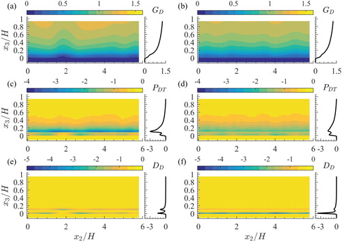
Figure 4. Spatial distributions of the transport terms of the DMKE balance of Eq. (3(3) $\begin{array}{rl}& \underset{\left(1\right):C_{DD}}{\underbrace{\frac{1}{2}\frac{\mathrm{\partial }}{\mathrm{\partial }{x}_j}({\phi }_{VT}⟨{\overline{u}}_i⟩⟨{\overline{u}}_i⟩⟨{\overline{u}}_j⟩)}}+\underset{\left(2\right):C_{DM}}{\underbrace{\frac{\mathrm{\partial }}{\mathrm{\partial }{x}_j}({\phi }_{Vm}⟨{\phi }_T{\tilde{\overline{u}}}_i⟩⟨{\overline{u}}_i⟩⟨{\overline{u}}_j⟩)}}\\ & =\underset{\left(3\right):G_D}{\underbrace{{\phi }_{VT}⟨{\overline{u}}_1⟩f_1}}-\underset{\left(4\right):-T_{DT}}{\underbrace{\frac{\mathrm{\partial }}{\mathrm{\partial }{x}_j}({\phi }_{Vm}⟨{\phi }_T\overline{u_i^{\mathrm{\prime }}{u}_j^{\mathrm{\prime }}}⟩⟨{\overline{u}}_i⟩)}}\\ & -\underset{\left(5\right):-T_{DF}}{\underbrace{\frac{\mathrm{\partial }}{\mathrm{\partial }{x}_j}({\phi }_{Vm}⟨{\phi }_T{\tilde{\overline{u}}}_i{\tilde{\overline{u}}}_j⟩⟨{\overline{u}}_i⟩)}}-\underset{\left(6\right):-T_{DM}}{\underbrace{\frac{1}{2}\frac{\mathrm{\partial }}{\mathrm{\partial }{x}_j}({\phi }_{Vm}⟨{\phi }_T{\tilde{\overline{u}}}_j⟩⟨{\overline{u}}_i⟩⟨{\overline{u}}_i⟩)}}\\ & -\underset{\left(7\right):-T_{DP}}{\underbrace{\frac{1}{{\rho }_f}\frac{\mathrm{\partial }}{\mathrm{\partial }{x}_i}({\phi }_{Vm}⟨{\phi }_T\overline{p}⟩⟨{\overline{u}}_i⟩)}}+\underset{\left(8\right):T_{DV}}{\underbrace{{\nu }_f\frac{\mathrm{\partial }}{\mathrm{\partial }{x}_j}({\phi }_{Vm}⟨{\phi }_T\overline{\frac{\mathrm{\partial }{u}_i}{\mathrm{\partial }{x}_j}}⟩⟨{\overline{u}}_i⟩)}}\\ & +\underset{\left(9\right):P_{DT}}{\underbrace{{\phi }_{Vm}⟨{\phi }_T\overline{u_i^{\mathrm{\prime }}{u}_j^{\mathrm{\prime }}}⟩\frac{\mathrm{\partial }⟨{\overline{u}}_i⟩}{\mathrm{\partial }{x}_j}}}+\underset{\left(10\right):P_{DF}}{\underbrace{{\phi }_{Vm}⟨{\phi }_T{\tilde{\overline{u}}}_i{\tilde{\overline{u}}}_j⟩\frac{\mathrm{\partial }⟨{\overline{u}}_i⟩}{\mathrm{\partial }{x}_j}}}\\ & +\underset{\left(11\right):P_{DM}}{\underbrace{{\phi }_{Vm}⟨{\phi }_T{\tilde{\overline{u}}}_i⟩⟨{\overline{u}}_j⟩\frac{\mathrm{\partial }⟨{\overline{u}}_i⟩}{\mathrm{\partial }{x}_j}}}\\ & +\underset{\left(12\right):P_{DP}}{\underbrace{\frac{{\phi }_{Vm}⟨{\phi }_T\overline{p}⟩}{{\rho }_f}\frac{\mathrm{\partial }⟨{\overline{u}}_i⟩}{\mathrm{\partial }{x}_i}}}-\underset{\left(13\right):-D_D}{\underbrace{{\nu }_f{\phi }_{Vm}⟨{\phi }_T\overline{\frac{\mathrm{\partial }{u}_i}{\mathrm{\partial }{x}_j}}⟩\frac{\mathrm{\partial }⟨{\overline{u}}_i⟩}{\mathrm{\partial }{x}_j}}}\\ & +\underset{\left(14\right):{\Phi }_D}{\underbrace{\frac{⟨{\overline{u}}_i⟩}{{\rho }_f{V}_0}{\overline{{\int }_{S_{int}}p{n}_i\mathrm{d}S}}^s-\frac{⟨{\overline{u}}_i⟩}{V_0}{\overline{{\int }_{S_{int}}{\nu }_f\frac{\mathrm{\partial }{u}_i}{\mathrm{\partial }{x}_j}{n}_j\mathrm{d}S}}^s}}\end{array}$(3) ): mean convection $C_{DD}$ (term 1) for scenarios HP (a) and LP (b); turbulent transport $T_{DT}$ (term 4) for scenarios HP (c) and LP (d); viscous transport $T_{DV}$ (term 8) for scenarios HP (e) and LP (f). The term values are normalized on $f_1{U}_b$

The spatial distribution of the local estimates of the energy supply $G_D$ (term 3, Fig. 3a and b) resembles the distribution of the streamwise double-averaged velocity reported in Vowinckel et al. (2017b), as expected. In the outer flow region, the distribution of $G_D$ is fairly homogeneous for scenario LP but shows some heterogeneity for scenario HP. In the latter case, it is evident that there is a significant effect of particle clusters on this term, especially at $x_2\approx 2H$ and $x_2\approx 4H$. Overall, the magnitude of the energy supply decreases with decreasing distance from the bed.

Part of the external energy is extracted and transferred to the turbulent energy budget due to the turbulent work $P_{DT}$ on the double-mean strain-rate (term 9; Fig. 3c and d). For both scenarios, the turbulence production (i.e. energy transfer to turbulence) increases towards the bed (due to the respective increase of the Reynolds stresses and velocity gradient), attaining its major peak within the particle mobility region. For scenario HP, this peak occurs at $x_3\approx 0.1H$, at the top of the particle clusters, while at $0<x_3<0.1H$ local increases of turbulence production are noted on the left and on the right of the clusters formed at $x_2\approx 2H$ and $4H$. For scenario LP, turbulence production peaks at $x_3\approx 0$ and 0.11H, particularly on the left-hand and right-hand sides of distinct low-valued regions at $x_2\approx 0.6H$, 2.1H, 3.8H and 5.3H. The observed spatial heterogeneity is reflected as the double-peak shape of the distribution of the global estimates of term 9.

The conversion of DMKE to heat (term 13) due to viscous stresses is stronger for scenario LP at $x_3=0$ (Fig. 3e and f). For scenario HP, heat conversion is enhanced at the top, left and right sides of the stable particle cluster (at $x_2\approx 2H$ and $0<x_3<0.1H$; Fig. 3e). For scenario LP, at $x_3\approx 0.1H$, viscous dissipation is locally enhanced in thin regions at $x_2\approx 0.6H$, 2.1H, 3.8H and 5.3H. This is reflected as a much weaker peak at $x_3\approx 0.1H$ in the distribution of its global counterpart (Fig. 3f).

The flow heterogeneity can be also noted in the spatial distributions of the convective, turbulent and viscous transport terms (Fig. 4). There are spots where estimates of the mean convection of DMKE (term 1) attain fairly large positive or negative values that well exceed those of the global estimates of the same quantity (Fig. 4a and b). The reason for this is the high heterogeneity of the local estimates in the spanwise direction. The areas of enhanced values of term 1 are larger for scenario HP, especially in the flow region near the particle cluster located at $x_2\approx 2H$. This feature hints to an effect of the secondary currents on mean energy transfers. The existence of secondary currents in this flow scenario has been highlighted in Vowinckel et al. (2017b). Turbulent transport (term 4) is also affected by the spanwise bed heterogeneity (Fig. 4c and d). For scenario HP, the highest values can be found at $x_3\approx 0.1H$ that corresponds to the top of the particle clusters formed around the positions $x_2\approx 2H$ and $x_2\approx 4H$. In addition, it is notable that turbulent transport is higher between the clusters, within the layer $0<x_3<0.1H$. For scenario LP, the magnitude of the turbulent transport is generally lower (as expected due to lower shear primary turbulent stress noted for this scenario). Nevertheless, turbulent transport is significant in the zone where particles move. Four distinct regions with smaller values can be noted at $x_3\approx 0.05H$ around $x_2\approx 0.6H$, 2.1H, 3.8H and 5.3H (Fig. 4d). These locations of reduced turbulent transport coincide with positions where local maxima of $⟨{\phi }_T⟩$ are observed (Vowinckel et al., 2017b). The local viscous stress transport (term 8) for scenario HP becomes significant near $x_3=0$ (i.e. at the level of fixed-particles' tops) on the left and on the right of the cluster formed at $x_2\approx 2H$ (Fig. 4e). Due to the formation of particle clusters, viscous effects are enhanced at $x_3\approx 0.1H$, on the top of the stable clusters. For scenario LP, the spanwise distribution of local values of viscous term 8 in Eq. (3(3) $\begin{array}{rl}& \underset{\left(1\right):C_{DD}}{\underbrace{\frac{1}{2}\frac{\mathrm{\partial }}{\mathrm{\partial }{x}_j}({\phi }_{VT}⟨{\overline{u}}_i⟩⟨{\overline{u}}_i⟩⟨{\overline{u}}_j⟩)}}+\underset{\left(2\right):C_{DM}}{\underbrace{\frac{\mathrm{\partial }}{\mathrm{\partial }{x}_j}({\phi }_{Vm}⟨{\phi }_T{\tilde{\overline{u}}}_i⟩⟨{\overline{u}}_i⟩⟨{\overline{u}}_j⟩)}}\\ & =\underset{\left(3\right):G_D}{\underbrace{{\phi }_{VT}⟨{\overline{u}}_1⟩f_1}}-\underset{\left(4\right):-T_{DT}}{\underbrace{\frac{\mathrm{\partial }}{\mathrm{\partial }{x}_j}({\phi }_{Vm}⟨{\phi }_T\overline{u_i^{\mathrm{\prime }}{u}_j^{\mathrm{\prime }}}⟩⟨{\overline{u}}_i⟩)}}\\ & -\underset{\left(5\right):-T_{DF}}{\underbrace{\frac{\mathrm{\partial }}{\mathrm{\partial }{x}_j}({\phi }_{Vm}⟨{\phi }_T{\tilde{\overline{u}}}_i{\tilde{\overline{u}}}_j⟩⟨{\overline{u}}_i⟩)}}-\underset{\left(6\right):-T_{DM}}{\underbrace{\frac{1}{2}\frac{\mathrm{\partial }}{\mathrm{\partial }{x}_j}({\phi }_{Vm}⟨{\phi }_T{\tilde{\overline{u}}}_j⟩⟨{\overline{u}}_i⟩⟨{\overline{u}}_i⟩)}}\\ & -\underset{\left(7\right):-T_{DP}}{\underbrace{\frac{1}{{\rho }_f}\frac{\mathrm{\partial }}{\mathrm{\partial }{x}_i}({\phi }_{Vm}⟨{\phi }_T\overline{p}⟩⟨{\overline{u}}_i⟩)}}+\underset{\left(8\right):T_{DV}}{\underbrace{{\nu }_f\frac{\mathrm{\partial }}{\mathrm{\partial }{x}_j}({\phi }_{Vm}⟨{\phi }_T\overline{\frac{\mathrm{\partial }{u}_i}{\mathrm{\partial }{x}_j}}⟩⟨{\overline{u}}_i⟩)}}\\ & +\underset{\left(9\right):P_{DT}}{\underbrace{{\phi }_{Vm}⟨{\phi }_T\overline{u_i^{\mathrm{\prime }}{u}_j^{\mathrm{\prime }}}⟩\frac{\mathrm{\partial }⟨{\overline{u}}_i⟩}{\mathrm{\partial }{x}_j}}}+\underset{\left(10\right):P_{DF}}{\underbrace{{\phi }_{Vm}⟨{\phi }_T{\tilde{\overline{u}}}_i{\tilde{\overline{u}}}_j⟩\frac{\mathrm{\partial }⟨{\overline{u}}_i⟩}{\mathrm{\partial }{x}_j}}}\\ & +\underset{\left(11\right):P_{DM}}{\underbrace{{\phi }_{Vm}⟨{\phi }_T{\tilde{\overline{u}}}_i⟩⟨{\overline{u}}_j⟩\frac{\mathrm{\partial }⟨{\overline{u}}_i⟩}{\mathrm{\partial }{x}_j}}}\\ & +\underset{\left(12\right):P_{DP}}{\underbrace{\frac{{\phi }_{Vm}⟨{\phi }_T\overline{p}⟩}{{\rho }_f}\frac{\mathrm{\partial }⟨{\overline{u}}_i⟩}{\mathrm{\partial }{x}_i}}}-\underset{\left(13\right):-D_D}{\underbrace{{\nu }_f{\phi }_{Vm}⟨{\phi }_T\overline{\frac{\mathrm{\partial }{u}_i}{\mathrm{\partial }{x}_j}}⟩\frac{\mathrm{\partial }⟨{\overline{u}}_i⟩}{\mathrm{\partial }{x}_j}}}\\ & +\underset{\left(14\right):{\Phi }_D}{\underbrace{\frac{⟨{\overline{u}}_i⟩}{{\rho }_f{V}_0}{\overline{{\int }_{S_{int}}p{n}_i\mathrm{d}S}}^s-\frac{⟨{\overline{u}}_i⟩}{V_0}{\overline{{\int }_{S_{int}}{\nu }_f\frac{\mathrm{\partial }{u}_i}{\mathrm{\partial }{x}_j}{n}_j\mathrm{d}S}}^s}}\end{array}$(3) ) is more homogeneous at $x_3\approx 0$ compared to the HP case, with even higher transverse homogeneity at $x_3\approx 0.1H$ (Fig. 4f).

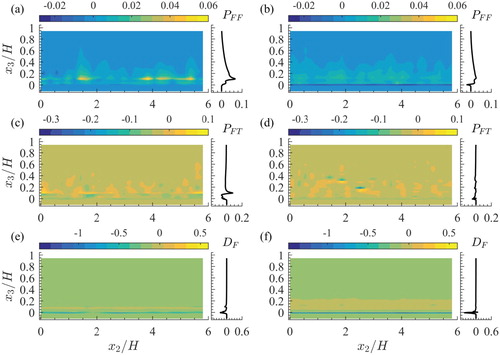
3.2. Budget of the form-induced kinetic energy

3.2.1. Relative significance of the terms in the FKE budget: globally averaged quantities

Figure 5 presents the spatial distributions of the estimates of the terms involved in the FKE budget (Eq. 4(4) $\begin{array}{rl}& \underset{\left(1\right):C_{FD}}{\underbrace{\frac{1}{2}\frac{\mathrm{\partial }}{\mathrm{\partial }{x}_j}({\phi }_{Vm}⟨{\phi }_T{\tilde{\overline{u}}}_i{\tilde{\overline{u}}}_i⟩⟨{\overline{u}}_j⟩)}}\\ & =\underset{\left(2\right):G_F}{\underbrace{{\phi }_{Vm}⟨{\phi }_T{\tilde{\overline{u}}}_1⟩f_1}}-\underset{\left(3\right):-P_{FF}}{\underbrace{{\phi }_{Vm}⟨{\phi }_T{\tilde{\overline{u}}}_i{\tilde{\overline{u}}}_j⟩\frac{⟨{\overline{u}}_i⟩}{\mathrm{\partial }{x}_j}}}\\ & -\underset{\left(4\right):-P_{FM}}{\underbrace{{\phi }_{Vm}⟨{\phi }_T{\tilde{\overline{u}}}_i⟩⟨{\overline{u}}_j⟩\frac{\mathrm{\partial }⟨{\overline{u}}_i⟩}{\mathrm{\partial }{x}_j}}}-\underset{\left(5\right):-T_{FF}}{\underbrace{\frac{1}{2}\frac{\mathrm{\partial }}{\mathrm{\partial }{x}_j}({\phi }_{Vm}⟨{\phi }_T{\tilde{\overline{u}}}_i{\tilde{\overline{u}}}_i{\tilde{\overline{u}}}_j⟩)}}\\ & -\underset{\left(6\right):-T_{FF}}{\underbrace{\frac{\mathrm{\partial }}{\mathrm{\partial }{x}_j}({\phi }_{Vm}⟨{\phi }_T\overline{u_i^{\mathrm{\prime }}{u}_j^{\mathrm{\prime }}}{\tilde{\overline{u}}}_i⟩)}}-\underset{\left(7\right):-T_{FP}}{\underbrace{\frac{1}{{\rho }_f}\frac{\mathrm{\partial }}{\mathrm{\partial }{x}_i}({\phi }_{Vm}⟨{\phi }_T\overline{p}{\tilde{\overline{u}}}_i⟩)}}\\ & +\underset{\left(8\right):T_{FV}}{\underbrace{{\nu }_f\frac{\mathrm{\partial }}{\mathrm{\partial }{x}_j}({\phi }_{Vm}⟨{\phi }_T\overline{\frac{\mathrm{\partial }{u}_i}{\mathrm{\partial }{x}_j}}{\tilde{\overline{u}}}_i⟩)}}+\underset{\left(9\right):P_{FT}}{\underbrace{{\phi }_{Vm}⟨{\phi }_T\overline{u_i^{\mathrm{\prime }}{u}_j^{\mathrm{\prime }}}\frac{\mathrm{\partial }{\tilde{\overline{u}}}_i}{\mathrm{\partial }{x}_j}⟩}}\\ & +\underset{\left(10\right):P_{FP}}{\underbrace{\frac{{\phi }_{Vm}}{{\rho }_f}⟨{\phi }_T\overline{p}\frac{\mathrm{\partial }{\tilde{\overline{u}}}_i}{\mathrm{\partial }{x}_i}⟩}}-\underset{\left(11\right):-D_F}{\underbrace{{\nu }_f{\phi }_{Vm}⟨{\phi }_T\overline{\frac{\mathrm{\partial }{u}_i}{\mathrm{\partial }{x}_j}}\frac{\mathrm{\partial }{\tilde{\overline{u}}}_i}{\mathrm{\partial }{x}_j}⟩}}\\ & +\underset{\left(12\right):{\Phi }_F}{\underbrace{\frac{1}{{\rho }_f{V}_0}{\overline{{\int }_{S_{int}}{\tilde{\overline{u}}}_{i}p{n}_i\mathrm{d}S}}^s-\frac{1}{V_0}{\overline{{\int }_{S_{int}}{\nu }_f{\tilde{\overline{u}}}_i\frac{\mathrm{\partial }{u}_i}{\mathrm{\partial }{x}_j}{n}_j\mathrm{d}S}}^s}}\end{array}$(4) ), following the global averaging scheme. It shows that the relative significance of the terms noticeably differs between the two scenarios. The effects of the terms associated with form-induced ($T_{FF}$) and turbulent ($T_{FT}$) fluxes are stronger for scenario HP compared to scenario LP (due to weaker Reynolds and form-induced stresses in scenario LP). The terms related to viscous stresses ($T_{FV}$) and pressure ($T_{FP}$) are more significant for scenario LP and dominate the mechanisms that control the variation of the FKE (Fig. 5a–d).

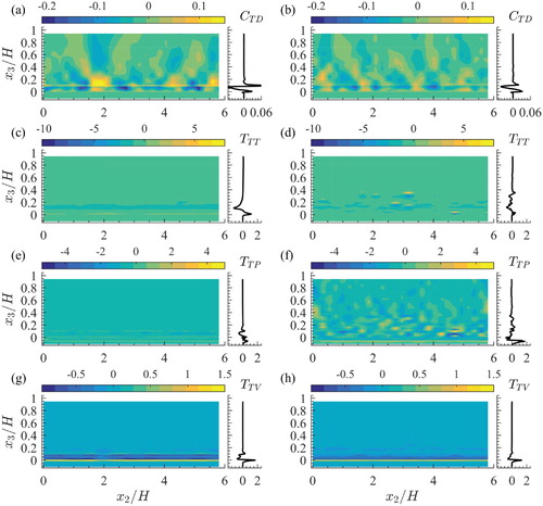
Figure 5. Vertical distributions of the terms of the globally averaged FKE balance of Eq. (4(4) $\begin{array}{rl}& \underset{\left(1\right):C_{FD}}{\underbrace{\frac{1}{2}\frac{\mathrm{\partial }}{\mathrm{\partial }{x}_j}({\phi }_{Vm}⟨{\phi }_T{\tilde{\overline{u}}}_i{\tilde{\overline{u}}}_i⟩⟨{\overline{u}}_j⟩)}}\\ & =\underset{\left(2\right):G_F}{\underbrace{{\phi }_{Vm}⟨{\phi }_T{\tilde{\overline{u}}}_1⟩f_1}}-\underset{\left(3\right):-P_{FF}}{\underbrace{{\phi }_{Vm}⟨{\phi }_T{\tilde{\overline{u}}}_i{\tilde{\overline{u}}}_j⟩\frac{⟨{\overline{u}}_i⟩}{\mathrm{\partial }{x}_j}}}\\ & -\underset{\left(4\right):-P_{FM}}{\underbrace{{\phi }_{Vm}⟨{\phi }_T{\tilde{\overline{u}}}_i⟩⟨{\overline{u}}_j⟩\frac{\mathrm{\partial }⟨{\overline{u}}_i⟩}{\mathrm{\partial }{x}_j}}}-\underset{\left(5\right):-T_{FF}}{\underbrace{\frac{1}{2}\frac{\mathrm{\partial }}{\mathrm{\partial }{x}_j}({\phi }_{Vm}⟨{\phi }_T{\tilde{\overline{u}}}_i{\tilde{\overline{u}}}_i{\tilde{\overline{u}}}_j⟩)}}\\ & -\underset{\left(6\right):-T_{FF}}{\underbrace{\frac{\mathrm{\partial }}{\mathrm{\partial }{x}_j}({\phi }_{Vm}⟨{\phi }_T\overline{u_i^{\mathrm{\prime }}{u}_j^{\mathrm{\prime }}}{\tilde{\overline{u}}}_i⟩)}}-\underset{\left(7\right):-T_{FP}}{\underbrace{\frac{1}{{\rho }_f}\frac{\mathrm{\partial }}{\mathrm{\partial }{x}_i}({\phi }_{Vm}⟨{\phi }_T\overline{p}{\tilde{\overline{u}}}_i⟩)}}\\ & +\underset{\left(8\right):T_{FV}}{\underbrace{{\nu }_f\frac{\mathrm{\partial }}{\mathrm{\partial }{x}_j}({\phi }_{Vm}⟨{\phi }_T\overline{\frac{\mathrm{\partial }{u}_i}{\mathrm{\partial }{x}_j}}{\tilde{\overline{u}}}_i⟩)}}+\underset{\left(9\right):P_{FT}}{\underbrace{{\phi }_{Vm}⟨{\phi }_T\overline{u_i^{\mathrm{\prime }}{u}_j^{\mathrm{\prime }}}\frac{\mathrm{\partial }{\tilde{\overline{u}}}_i}{\mathrm{\partial }{x}_j}⟩}}\\ & +\underset{\left(10\right):P_{FP}}{\underbrace{\frac{{\phi }_{Vm}}{{\rho }_f}⟨{\phi }_T\overline{p}\frac{\mathrm{\partial }{\tilde{\overline{u}}}_i}{\mathrm{\partial }{x}_i}⟩}}-\underset{\left(11\right):-D_F}{\underbrace{{\nu }_f{\phi }_{Vm}⟨{\phi }_T\overline{\frac{\mathrm{\partial }{u}_i}{\mathrm{\partial }{x}_j}}\frac{\mathrm{\partial }{\tilde{\overline{u}}}_i}{\mathrm{\partial }{x}_j}⟩}}\\ & +\underset{\left(12\right):{\Phi }_F}{\underbrace{\frac{1}{{\rho }_f{V}_0}{\overline{{\int }_{S_{int}}{\tilde{\overline{u}}}_{i}p{n}_i\mathrm{d}S}}^s-\frac{1}{V_0}{\overline{{\int }_{S_{int}}{\nu }_f{\tilde{\overline{u}}}_i\frac{\mathrm{\partial }{u}_i}{\mathrm{\partial }{x}_j}{n}_j\mathrm{d}S}}^s}}\end{array}$(4) ): mean $C_{FD}$ (term 1) and form-induced convection of FKE $T_{FF}$ (term 5) for scenarios HP (a) and LP (b); turbulent $T_{FT}$ (term 6), pressure $T_{FP}$ (term 7) and viscous stress transport $T_{FV}$ (term 8) for scenarios HP (c) and LP (d); energy supply $G_F$ (term 2) and interfacial energy exchange ${\Phi }_F$ (term 12) for scenarios HP (e) and LP (f); energy exchange with the DMKE balance $P_{FF}$ (term 3), $P_{FM}$ (term 4) and TKE balance $P_{FT}$ (term 9) for scenarios HP (g) and LP (h); the work of pressure on the form-induced strain rate $P_{FP}$ (term 10), viscous dissipation to heat $D_F$ (term 11) for the scenarios HP (i) and LP (j). The term values are normalized on $f_1{U}_b$

For both scenarios, the primary supply of energy to the form-induced velocity field relates to the particle motion (term 12, ${\Phi }_F$; Fig. 5e and f). The secondary energy supply is from the double-mean flow due to the work of $⟨{\tilde{\overline{u}}}_1{\tilde{\overline{u}}}_3⟩$ on the double-mean strain rate (term 3, $P_{FF}$; Fig. 5g and h). For scenario LP, the energy supply coming from the interfacial term ${\Phi }_F$ is much stronger than for scenario HP (term 12; Fig. 5f); for both scenarios it becomes noticeable below $x_3\approx 0.02H$. Part of this energy supply is dissipated directly into heat due to the work of viscous stresses (term 11, $D_F$; particularly profound for the LP case, Fig. 5j), or removed due to the work of pressure (terms 7, $T_{FP}$ and 10, $P_{FP}$; Fig. 5d and j). For $0.02H<x_3<0.5H$, the kinetic energy is also supplied by the double-mean velocity field, due to the work of form-induced stresses on the double-mean strain-rate (term 3, $P_{FF}$; Fig. 5g and h).

For scenario HP, the FKE produced in the region $0\le x_3\le 0.1H$ is removed due to the work of turbulent (term 9, $P_{FT}$) and viscous stresses (term 11, $D_F$) on the form-induced strain rate (Fig. 5g and i). The sign of term 9 ($P_{FT}$) for the HP case is negative at $x_3<0.08H$ and $0.13H<x_3<0.58H$ and positive at $0.08H<x_3<0.13H$. This suggests that FKE receives energy from turbulent motions in a thin layer above the cluster tops, while below and above that layer the form-induced flow field supplies energy to the turbulent flow field. The magnitude of term 9 ($P_{FT}$) is comparable to the magnitude of term 3 ($P_{FF}$), particularly for the HP case. For scenario LP, the effect of terms 3 and 9 is not significant. The most significant components of the exchange between turbulent and form-induced fields (term 9) involve the work of the primary shear Reynolds stress $\overline{u_1^{\mathrm{\prime }}{u}_3^{\mathrm{\prime }}}$ (not reported in the figures of this paper). Similar observations on the behaviour of these terms are made in Yuan and Piomelli (2014) for the case of fixed-bed flow, where the authors suggest that for the length scales larger than the roughness height, turbulent energy is converted into the energy of the form-induced flow. The overall effect of the viscous stresses work on the form-induced strain-rate ($D_F$) is dissipative and it is significant in a thin layer in the vicinity of $x_3\approx 0$ and $x_3\approx 0.1H$ (Fig. 5i and j).

The convection terms (terms 1 and 5; Fig. 5a and b) are far weaker than the turbulent, pressure and viscous transport terms (terms 6, 7 and 8; Fig. 5c and d) for both scenarios. For scenario HP, mean convection (term 1, $C_{FD}$) transfers the FKE from thin regions close to $x_3=0$ and 0.08H to a thin layer just above $x_3\approx 0$, while the energy supplied within $0<x_3<0.1H$ is transferred due to the work of viscous stress (term 8, $T_{FV}$) in thin layers near $x_3=0$ and $x_3=0.1H$ (Fig. 5c). Mean convective transport for case LP is insignificant. Pressure transport for scenario HP (term 7, $T_{FP}$; Fig. 5c) is far weaker than turbulent (term 6, $T_{FT}$) and viscous (term 8, $T_{FV}$) transport and its contribution is positive at $x_3\approx 0$ and 0.1H. Hence, an approximate balance can be noted between the pressure, turbulent and viscous transport terms for scenario HP (Fig. 5c). The weaker transport terms of mean (term 1) and form-induced convection (term 5) also counter each other's effects (Fig. 5a). For scenario LP, most of energy is supplied to the FKE balance by particle motion and the double-mean flow field (term 12, ${\Phi }_F$; Fig. 5f), while pressure (term 7, $T_{FP}$; Fig. 5d) and viscous (term 8, $T_{FV}$; Fig. 5d) transport terms are those that are responsible for the spatial redistribution of FKE. Pressure transport removes energy from a thin flow layer at $x_3=0$ to a thin region just above. Viscous transport has the opposite effect, as it transfers energy close to the particle tops. The contribution of pressure work on mean strain rate (term 10, $P_{FP}$; Fig. 5j) is significantly increased for scenario LP. In a thin layer just above $x_3\approx 0$, $P_{FP}$ (term 10) removes energy from the budget, while in a thin layer at $x_3\approx 0$ it brings energy to the form-induced flow.

3.2.2. Spatial variability of the terms in the FKE budget: locally averaged quantities

The sign of the energy exchange (term 3, $P_{FF}$) is mainly positive for both scenarios (Fig. 6a and b), highlighting that the work of form-induced stresses on the double-mean strain-rate mainly converts DMKE to FKE. For scenario HP, this energy conversion is locally enhanced at the top of the particles clusters, at $x_2\approx 0.5H$, 1.8H, 3.2H, 4.1H and within the layer $0<x_2<0.2H$. For scenario LP, there are locations at the top of the fixed-particles where the sign of $P_{FF}$ (term 3) becomes negative, suggesting the dissipative effect of the term that converts FKE to DMKE. The work of the Reynolds stress on the form-induced strain rate (term 9, $P_{FT}$) “dissipates” energy within the region $0<x_3<0.1H$ and its dissipative effect peaks near the particle clusters of scenario HP (Fig. 6c). In thin regions at the tops of the HP clusters, at $x_2\approx 0.5H$, 1.8H, 3.2H, 4.1H, the contribution of $P_{FT}$ (term 9) becomes positive, reflecting the gain of FKE. The role of term $P_{FT}$ in scenario LP is not clear, as its value is generally negligible, although some noticeable peaks are observed at $x_2\approx 1.7H$, 2.1H for $x_3\approx 0.3H$ and at $x_2\approx 2.8H$ for $x_3\approx 0.2H$ (Fig. 6d). The work of the viscous stresses on the form-induced strain rate (term 11; $D_F$; Fig. 6e and f) is negative, i.e. it dissipates energy near the level of $x_3=0$ for both scenarios, with the term's magnitude being higher for scenario LP. For scenario LP, thin layers where the sign of $D_F$ is positive, are found below and above the level $x_3\approx 0$ and at $x_3\approx 0.1H$, suggesting that the term's contribution to the FKE balance may attain positive values too.

Figure 6. Spatial distributions of the energy converting terms of the FKE balance of Eq. (4(4) $\begin{array}{rl}& \underset{\left(1\right):C_{FD}}{\underbrace{\frac{1}{2}\frac{\mathrm{\partial }}{\mathrm{\partial }{x}_j}({\phi }_{Vm}⟨{\phi }_T{\tilde{\overline{u}}}_i{\tilde{\overline{u}}}_i⟩⟨{\overline{u}}_j⟩)}}\\ & =\underset{\left(2\right):G_F}{\underbrace{{\phi }_{Vm}⟨{\phi }_T{\tilde{\overline{u}}}_1⟩f_1}}-\underset{\left(3\right):-P_{FF}}{\underbrace{{\phi }_{Vm}⟨{\phi }_T{\tilde{\overline{u}}}_i{\tilde{\overline{u}}}_j⟩\frac{⟨{\overline{u}}_i⟩}{\mathrm{\partial }{x}_j}}}\\ & -\underset{\left(4\right):-P_{FM}}{\underbrace{{\phi }_{Vm}⟨{\phi }_T{\tilde{\overline{u}}}_i⟩⟨{\overline{u}}_j⟩\frac{\mathrm{\partial }⟨{\overline{u}}_i⟩}{\mathrm{\partial }{x}_j}}}-\underset{\left(5\right):-T_{FF}}{\underbrace{\frac{1}{2}\frac{\mathrm{\partial }}{\mathrm{\partial }{x}_j}({\phi }_{Vm}⟨{\phi }_T{\tilde{\overline{u}}}_i{\tilde{\overline{u}}}_i{\tilde{\overline{u}}}_j⟩)}}\\ & -\underset{\left(6\right):-T_{FF}}{\underbrace{\frac{\mathrm{\partial }}{\mathrm{\partial }{x}_j}({\phi }_{Vm}⟨{\phi }_T\overline{u_i^{\mathrm{\prime }}{u}_j^{\mathrm{\prime }}}{\tilde{\overline{u}}}_i⟩)}}-\underset{\left(7\right):-T_{FP}}{\underbrace{\frac{1}{{\rho }_f}\frac{\mathrm{\partial }}{\mathrm{\partial }{x}_i}({\phi }_{Vm}⟨{\phi }_T\overline{p}{\tilde{\overline{u}}}_i⟩)}}\\ & +\underset{\left(8\right):T_{FV}}{\underbrace{{\nu }_f\frac{\mathrm{\partial }}{\mathrm{\partial }{x}_j}({\phi }_{Vm}⟨{\phi }_T\overline{\frac{\mathrm{\partial }{u}_i}{\mathrm{\partial }{x}_j}}{\tilde{\overline{u}}}_i⟩)}}+\underset{\left(9\right):P_{FT}}{\underbrace{{\phi }_{Vm}⟨{\phi }_T\overline{u_i^{\mathrm{\prime }}{u}_j^{\mathrm{\prime }}}\frac{\mathrm{\partial }{\tilde{\overline{u}}}_i}{\mathrm{\partial }{x}_j}⟩}}\\ & +\underset{\left(10\right):P_{FP}}{\underbrace{\frac{{\phi }_{Vm}}{{\rho }_f}⟨{\phi }_T\overline{p}\frac{\mathrm{\partial }{\tilde{\overline{u}}}_i}{\mathrm{\partial }{x}_i}⟩}}-\underset{\left(11\right):-D_F}{\underbrace{{\nu }_f{\phi }_{Vm}⟨{\phi }_T\overline{\frac{\mathrm{\partial }{u}_i}{\mathrm{\partial }{x}_j}}\frac{\mathrm{\partial }{\tilde{\overline{u}}}_i}{\mathrm{\partial }{x}_j}⟩}}\\ & +\underset{\left(12\right):{\Phi }_F}{\underbrace{\frac{1}{{\rho }_f{V}_0}{\overline{{\int }_{S_{int}}{\tilde{\overline{u}}}_{i}p{n}_i\mathrm{d}S}}^s-\frac{1}{V_0}{\overline{{\int }_{S_{int}}{\nu }_f{\tilde{\overline{u}}}_i\frac{\mathrm{\partial }{u}_i}{\mathrm{\partial }{x}_j}{n}_j\mathrm{d}S}}^s}}\end{array}$(4) ): energy supply from the DMKE balance $P_{FF}$ (term 3) for scenarios HP (a) and LP (b); energy exchange with the TKE balance $P_{FT}$ (term 9) for scenarios HP (c) and LP (d); viscous dissipation $D_F$ (term 11) for the scenarios HP (e) and LP (f). The term values are normalized on $f_1{U}_b$

The effect of the mean convection (term 1, $C_{FD}$; Fig. 7a) for scenario HP is restricted to the layer $0<x_3<0.1H$, especially near the clusters formed at $x_2\approx 2H$ and $x_2\approx 4H$. For scenario LP, term 1 deviates from zero only at $x_2\approx 2.1H$, 2.8H and 3.8H (Fig. 7b), although its magnitudes are much smaller compared to HP. Similar alternating patterns due to particle clusters, as noted in the distribution of the local DMKE convection for scenario HP (term 1 in Eq. 3(3) $\begin{array}{rl}& \underset{\left(1\right):C_{DD}}{\underbrace{\frac{1}{2}\frac{\mathrm{\partial }}{\mathrm{\partial }{x}_j}({\phi }_{VT}⟨{\overline{u}}_i⟩⟨{\overline{u}}_i⟩⟨{\overline{u}}_j⟩)}}+\underset{\left(2\right):C_{DM}}{\underbrace{\frac{\mathrm{\partial }}{\mathrm{\partial }{x}_j}({\phi }_{Vm}⟨{\phi }_T{\tilde{\overline{u}}}_i⟩⟨{\overline{u}}_i⟩⟨{\overline{u}}_j⟩)}}\\ & =\underset{\left(3\right):G_D}{\underbrace{{\phi }_{VT}⟨{\overline{u}}_1⟩f_1}}-\underset{\left(4\right):-T_{DT}}{\underbrace{\frac{\mathrm{\partial }}{\mathrm{\partial }{x}_j}({\phi }_{Vm}⟨{\phi }_T\overline{u_i^{\mathrm{\prime }}{u}_j^{\mathrm{\prime }}}⟩⟨{\overline{u}}_i⟩)}}\\ & -\underset{\left(5\right):-T_{DF}}{\underbrace{\frac{\mathrm{\partial }}{\mathrm{\partial }{x}_j}({\phi }_{Vm}⟨{\phi }_T{\tilde{\overline{u}}}_i{\tilde{\overline{u}}}_j⟩⟨{\overline{u}}_i⟩)}}-\underset{\left(6\right):-T_{DM}}{\underbrace{\frac{1}{2}\frac{\mathrm{\partial }}{\mathrm{\partial }{x}_j}({\phi }_{Vm}⟨{\phi }_T{\tilde{\overline{u}}}_j⟩⟨{\overline{u}}_i⟩⟨{\overline{u}}_i⟩)}}\\ & -\underset{\left(7\right):-T_{DP}}{\underbrace{\frac{1}{{\rho }_f}\frac{\mathrm{\partial }}{\mathrm{\partial }{x}_i}({\phi }_{Vm}⟨{\phi }_T\overline{p}⟩⟨{\overline{u}}_i⟩)}}+\underset{\left(8\right):T_{DV}}{\underbrace{{\nu }_f\frac{\mathrm{\partial }}{\mathrm{\partial }{x}_j}({\phi }_{Vm}⟨{\phi }_T\overline{\frac{\mathrm{\partial }{u}_i}{\mathrm{\partial }{x}_j}}⟩⟨{\overline{u}}_i⟩)}}\\ & +\underset{\left(9\right):P_{DT}}{\underbrace{{\phi }_{Vm}⟨{\phi }_T\overline{u_i^{\mathrm{\prime }}{u}_j^{\mathrm{\prime }}}⟩\frac{\mathrm{\partial }⟨{\overline{u}}_i⟩}{\mathrm{\partial }{x}_j}}}+\underset{\left(10\right):P_{DF}}{\underbrace{{\phi }_{Vm}⟨{\phi }_T{\tilde{\overline{u}}}_i{\tilde{\overline{u}}}_j⟩\frac{\mathrm{\partial }⟨{\overline{u}}_i⟩}{\mathrm{\partial }{x}_j}}}\\ & +\underset{\left(11\right):P_{DM}}{\underbrace{{\phi }_{Vm}⟨{\phi }_T{\tilde{\overline{u}}}_i⟩⟨{\overline{u}}_j⟩\frac{\mathrm{\partial }⟨{\overline{u}}_i⟩}{\mathrm{\partial }{x}_j}}}\\ & +\underset{\left(12\right):P_{DP}}{\underbrace{\frac{{\phi }_{Vm}⟨{\phi }_T\overline{p}⟩}{{\rho }_f}\frac{\mathrm{\partial }⟨{\overline{u}}_i⟩}{\mathrm{\partial }{x}_i}}}-\underset{\left(13\right):-D_D}{\underbrace{{\nu }_f{\phi }_{Vm}⟨{\phi }_T\overline{\frac{\mathrm{\partial }{u}_i}{\mathrm{\partial }{x}_j}}⟩\frac{\mathrm{\partial }⟨{\overline{u}}_i⟩}{\mathrm{\partial }{x}_j}}}\\ & +\underset{\left(14\right):{\Phi }_D}{\underbrace{\frac{⟨{\overline{u}}_i⟩}{{\rho }_f{V}_0}{\overline{{\int }_{S_{int}}p{n}_i\mathrm{d}S}}^s-\frac{⟨{\overline{u}}_i⟩}{V_0}{\overline{{\int }_{S_{int}}{\nu }_f\frac{\mathrm{\partial }{u}_i}{\mathrm{\partial }{x}_j}{n}_j\mathrm{d}S}}^s}}\end{array}$(3) , Fig. 4a), are observed for $C_{FD}$ (term 1) in Eq. (4(4) $\begin{array}{rl}& \underset{\left(1\right):C_{FD}}{\underbrace{\frac{1}{2}\frac{\mathrm{\partial }}{\mathrm{\partial }{x}_j}({\phi }_{Vm}⟨{\phi }_T{\tilde{\overline{u}}}_i{\tilde{\overline{u}}}_i⟩⟨{\overline{u}}_j⟩)}}\\ & =\underset{\left(2\right):G_F}{\underbrace{{\phi }_{Vm}⟨{\phi }_T{\tilde{\overline{u}}}_1⟩f_1}}-\underset{\left(3\right):-P_{FF}}{\underbrace{{\phi }_{Vm}⟨{\phi }_T{\tilde{\overline{u}}}_i{\tilde{\overline{u}}}_j⟩\frac{⟨{\overline{u}}_i⟩}{\mathrm{\partial }{x}_j}}}\\ & -\underset{\left(4\right):-P_{FM}}{\underbrace{{\phi }_{Vm}⟨{\phi }_T{\tilde{\overline{u}}}_i⟩⟨{\overline{u}}_j⟩\frac{\mathrm{\partial }⟨{\overline{u}}_i⟩}{\mathrm{\partial }{x}_j}}}-\underset{\left(5\right):-T_{FF}}{\underbrace{\frac{1}{2}\frac{\mathrm{\partial }}{\mathrm{\partial }{x}_j}({\phi }_{Vm}⟨{\phi }_T{\tilde{\overline{u}}}_i{\tilde{\overline{u}}}_i{\tilde{\overline{u}}}_j⟩)}}\\ & -\underset{\left(6\right):-T_{FF}}{\underbrace{\frac{\mathrm{\partial }}{\mathrm{\partial }{x}_j}({\phi }_{Vm}⟨{\phi }_T\overline{u_i^{\mathrm{\prime }}{u}_j^{\mathrm{\prime }}}{\tilde{\overline{u}}}_i⟩)}}-\underset{\left(7\right):-T_{FP}}{\underbrace{\frac{1}{{\rho }_f}\frac{\mathrm{\partial }}{\mathrm{\partial }{x}_i}({\phi }_{Vm}⟨{\phi }_T\overline{p}{\tilde{\overline{u}}}_i⟩)}}\\ & +\underset{\left(8\right):T_{FV}}{\underbrace{{\nu }_f\frac{\mathrm{\partial }}{\mathrm{\partial }{x}_j}({\phi }_{Vm}⟨{\phi }_T\overline{\frac{\mathrm{\partial }{u}_i}{\mathrm{\partial }{x}_j}}{\tilde{\overline{u}}}_i⟩)}}+\underset{\left(9\right):P_{FT}}{\underbrace{{\phi }_{Vm}⟨{\phi }_T\overline{u_i^{\mathrm{\prime }}{u}_j^{\mathrm{\prime }}}\frac{\mathrm{\partial }{\tilde{\overline{u}}}_i}{\mathrm{\partial }{x}_j}⟩}}\\ & +\underset{\left(10\right):P_{FP}}{\underbrace{\frac{{\phi }_{Vm}}{{\rho }_f}⟨{\phi }_T\overline{p}\frac{\mathrm{\partial }{\tilde{\overline{u}}}_i}{\mathrm{\partial }{x}_i}⟩}}-\underset{\left(11\right):-D_F}{\underbrace{{\nu }_f{\phi }_{Vm}⟨{\phi }_T\overline{\frac{\mathrm{\partial }{u}_i}{\mathrm{\partial }{x}_j}}\frac{\mathrm{\partial }{\tilde{\overline{u}}}_i}{\mathrm{\partial }{x}_j}⟩}}\\ & +\underset{\left(12\right):{\Phi }_F}{\underbrace{\frac{1}{{\rho }_f{V}_0}{\overline{{\int }_{S_{int}}{\tilde{\overline{u}}}_{i}p{n}_i\mathrm{d}S}}^s-\frac{1}{V_0}{\overline{{\int }_{S_{int}}{\nu }_f{\tilde{\overline{u}}}_i\frac{\mathrm{\partial }{u}_i}{\mathrm{\partial }{x}_j}{n}_j\mathrm{d}S}}^s}}\end{array}$(4) ). No such effect is visible in the distribution of local $C_{FD}$ for scenario LP. Form-induced convection (term 5, $T_{FF}$; Fig. 7c) is non-zero within the layer $0<x_3<0.1H$ on the left and right sides of the stable particle cluster observed in scenario HP. The contribution of this term in scenario LP is much weaker and limited to a thin layer near $x_3\approx 0$ (Fig. 7d). Compared to HP, its distribution in the spanwise direction is less heterogeneous as one would expect for the case of intense and unstructured particle motion. Turbulent transport (term 6, $T_{FT}$; Fig. 7e) for scenario HP is also limited to the layer below $x_3\approx 0.1H$, being enhanced near the particle clusters. For scenario LP (Fig. 7f), the turbulent transport effect is, overall, noticeably weaker. However, some distinct spots where the magnitude of the term is quite high are noted near $x_2\approx 1.7H$, 2.1H for $x_3\approx 0.3H$ and at $x_2\approx 2.8H$ for $x_3\approx 0.2H$. Viscous transport (term 8, $T_{FV}$; Fig. 7g and h) for scenario HP is locally enhanced at the top of the particle clusters (i.e. at $x_3\approx 0.1H$) and at $x_3\approx 0$ on the left and right sides of the clusters. For scenario LP, however, this term is significant only near $x_3=0$, with no particular variations in the spanwise direction.

Figure 7. Spatial distributions of the transport terms of the FKE balance of Eq. (4(4) $\begin{array}{rl}& \underset{\left(1\right):C_{FD}}{\underbrace{\frac{1}{2}\frac{\mathrm{\partial }}{\mathrm{\partial }{x}_j}({\phi }_{Vm}⟨{\phi }_T{\tilde{\overline{u}}}_i{\tilde{\overline{u}}}_i⟩⟨{\overline{u}}_j⟩)}}\\ & =\underset{\left(2\right):G_F}{\underbrace{{\phi }_{Vm}⟨{\phi }_T{\tilde{\overline{u}}}_1⟩f_1}}-\underset{\left(3\right):-P_{FF}}{\underbrace{{\phi }_{Vm}⟨{\phi }_T{\tilde{\overline{u}}}_i{\tilde{\overline{u}}}_j⟩\frac{⟨{\overline{u}}_i⟩}{\mathrm{\partial }{x}_j}}}\\ & -\underset{\left(4\right):-P_{FM}}{\underbrace{{\phi }_{Vm}⟨{\phi }_T{\tilde{\overline{u}}}_i⟩⟨{\overline{u}}_j⟩\frac{\mathrm{\partial }⟨{\overline{u}}_i⟩}{\mathrm{\partial }{x}_j}}}-\underset{\left(5\right):-T_{FF}}{\underbrace{\frac{1}{2}\frac{\mathrm{\partial }}{\mathrm{\partial }{x}_j}({\phi }_{Vm}⟨{\phi }_T{\tilde{\overline{u}}}_i{\tilde{\overline{u}}}_i{\tilde{\overline{u}}}_j⟩)}}\\ & -\underset{\left(6\right):-T_{FF}}{\underbrace{\frac{\mathrm{\partial }}{\mathrm{\partial }{x}_j}({\phi }_{Vm}⟨{\phi }_T\overline{u_i^{\mathrm{\prime }}{u}_j^{\mathrm{\prime }}}{\tilde{\overline{u}}}_i⟩)}}-\underset{\left(7\right):-T_{FP}}{\underbrace{\frac{1}{{\rho }_f}\frac{\mathrm{\partial }}{\mathrm{\partial }{x}_i}({\phi }_{Vm}⟨{\phi }_T\overline{p}{\tilde{\overline{u}}}_i⟩)}}\\ & +\underset{\left(8\right):T_{FV}}{\underbrace{{\nu }_f\frac{\mathrm{\partial }}{\mathrm{\partial }{x}_j}({\phi }_{Vm}⟨{\phi }_T\overline{\frac{\mathrm{\partial }{u}_i}{\mathrm{\partial }{x}_j}}{\tilde{\overline{u}}}_i⟩)}}+\underset{\left(9\right):P_{FT}}{\underbrace{{\phi }_{Vm}⟨{\phi }_T\overline{u_i^{\mathrm{\prime }}{u}_j^{\mathrm{\prime }}}\frac{\mathrm{\partial }{\tilde{\overline{u}}}_i}{\mathrm{\partial }{x}_j}⟩}}\\ & +\underset{\left(10\right):P_{FP}}{\underbrace{\frac{{\phi }_{Vm}}{{\rho }_f}⟨{\phi }_T\overline{p}\frac{\mathrm{\partial }{\tilde{\overline{u}}}_i}{\mathrm{\partial }{x}_i}⟩}}-\underset{\left(11\right):-D_F}{\underbrace{{\nu }_f{\phi }_{Vm}⟨{\phi }_T\overline{\frac{\mathrm{\partial }{u}_i}{\mathrm{\partial }{x}_j}}\frac{\mathrm{\partial }{\tilde{\overline{u}}}_i}{\mathrm{\partial }{x}_j}⟩}}\\ & +\underset{\left(12\right):{\Phi }_F}{\underbrace{\frac{1}{{\rho }_f{V}_0}{\overline{{\int }_{S_{int}}{\tilde{\overline{u}}}_{i}p{n}_i\mathrm{d}S}}^s-\frac{1}{V_0}{\overline{{\int }_{S_{int}}{\nu }_f{\tilde{\overline{u}}}_i\frac{\mathrm{\partial }{u}_i}{\mathrm{\partial }{x}_j}{n}_j\mathrm{d}S}}^s}}\end{array}$(4) ): mean convection $C_{FD}$ (term 1) for scenarios HP (a) and LP (b); form-induced convection $T_{FF}$ (term 5) for scenarios HP (c) and LP (d); turbulent transport $T_{FT}$ (term 6) for scenarios HP (e) and LP (f); viscous transport $T_{FV}$ (term 8) for the scenarios HP (g) and LP (h). The values are normalized on $f_1{U}_b$

3.3. Budget of the spatially averaged turbulent energy

3.3.1. Relative significance of the terms of the TKE budget: globally averaged quantities

Vertical distributions of the globally averaged terms of the TKE balance (Eq. 5(5) $\begin{array}{rl}& \underset{\left(1\right):C_{TD}}{\underbrace{\frac{1}{2}\frac{\mathrm{\partial }}{\mathrm{\partial }{x}_j}({\phi }_{Vm}⟨{\phi }_T\overline{u_i^{\mathrm{\prime }}{u}_i^{\mathrm{\prime }}}⟩⟨{\overline{u}}_j⟩)}}\\ & =-\underset{\left(2\right):-P_{TT}}{\underbrace{{\phi }_{Vm}⟨{\phi }_T\overline{u_i^{\mathrm{\prime }}{u}_j^{\mathrm{\prime }}}⟩\frac{\mathrm{\partial }⟨{\overline{u}}_i⟩}{\mathrm{\partial }{x}_j}}}-\underset{\left(3\right):-P_{TF}}{\underbrace{{\phi }_{Vm}⟨{\phi }_T\overline{u_i^{\mathrm{\prime }}{u}_j^{\mathrm{\prime }}}\frac{\mathrm{\partial }{\tilde{\overline{u}}}_i}{\mathrm{\partial }{x}_j}⟩}}\\ & -\underset{\left(4\right):-T_{TF}}{\underbrace{\frac{1}{2}\frac{\mathrm{\partial }}{\mathrm{\partial }{x}_j}({\phi }_{Vm}⟨{\phi }_T\overline{u_i^{\mathrm{\prime }}{u}_i^{\mathrm{\prime }}}{\tilde{\overline{u}}}_j⟩)}}-\underset{\left(5\right):-T_{TT}}{\underbrace{\frac{1}{2}\frac{\mathrm{\partial }}{\mathrm{\partial }{x}_j}({\phi }_{Vm}⟨{\phi }_T\overline{u_i^{\mathrm{\prime }}{u}_i^{\mathrm{\prime }}{u}_j^{\mathrm{\prime }}}⟩)}}\\ & -\underset{\left(6\right):-T_{TP}}{\underbrace{\frac{1}{{\rho }_f}\frac{\mathrm{\partial }}{\mathrm{\partial }{x}_i}({\phi }_{Vm}⟨{\phi }_T\overline{u_i^{\mathrm{\prime }}{p}^{\mathrm{\prime }}}⟩)}}+\underset{\left(7\right):T_{TV}}{\underbrace{{\nu }_f\frac{\mathrm{\partial }}{\mathrm{\partial }{x}_j}\left({\phi }_{Vm}⟨{\phi }_T\overline{u_i^{\mathrm{\prime }}\frac{\mathrm{\partial }{u}_i^{\mathrm{\prime }}}{\mathrm{\partial }{x}_j}}⟩\right)}}\\ & +\underset{\left(8\right):P_{TP}}{\underbrace{\frac{{\phi }_{Vm}}{{\rho }_f}⟨{\phi }_T\overline{p^{\mathrm{\prime }}\frac{\mathrm{\partial }{u}_i^{\mathrm{\prime }}}{\mathrm{\partial }{x}_i}}⟩}}-\underset{\left(9\right):-D_T}{\underbrace{{\nu }_f{\phi }_{Vm}⟨{\phi }_T\overline{\frac{\mathrm{\partial }{u}_i^{\mathrm{\prime }}}{\mathrm{\partial }{x}_j}\frac{\mathrm{\partial }{u}_i^{\mathrm{\prime }}}{\mathrm{\partial }{x}_j}}⟩}}\\ & +\underset{\left(10\right):{\Phi }_T}{\underbrace{\frac{1}{{\rho }_f{V}_0}{\overline{{\int }_{S_{int}}{u}_i^{\mathrm{\prime }}p{n}_i\mathrm{d}S}}^s-\frac{1}{V_0}{\overline{{\int }_{S_{int}}{\nu }_f{u}_i^{\mathrm{\prime }}\frac{\mathrm{\partial }{u}_i}{\mathrm{\partial }{x}_j}{n}_j\mathrm{d}S}}^s}}\end{array}$(5) ) are shown in Fig. 8. Above the tops of the fixed bed particles, double-mean flow and particle motion supply kinetic energy to the turbulent velocity field through terms 2 and 10 of Eq. (5(5) $\begin{array}{rl}& \underset{\left(1\right):C_{TD}}{\underbrace{\frac{1}{2}\frac{\mathrm{\partial }}{\mathrm{\partial }{x}_j}({\phi }_{Vm}⟨{\phi }_T\overline{u_i^{\mathrm{\prime }}{u}_i^{\mathrm{\prime }}}⟩⟨{\overline{u}}_j⟩)}}\\ & =-\underset{\left(2\right):-P_{TT}}{\underbrace{{\phi }_{Vm}⟨{\phi }_T\overline{u_i^{\mathrm{\prime }}{u}_j^{\mathrm{\prime }}}⟩\frac{\mathrm{\partial }⟨{\overline{u}}_i⟩}{\mathrm{\partial }{x}_j}}}-\underset{\left(3\right):-P_{TF}}{\underbrace{{\phi }_{Vm}⟨{\phi }_T\overline{u_i^{\mathrm{\prime }}{u}_j^{\mathrm{\prime }}}\frac{\mathrm{\partial }{\tilde{\overline{u}}}_i}{\mathrm{\partial }{x}_j}⟩}}\\ & -\underset{\left(4\right):-T_{TF}}{\underbrace{\frac{1}{2}\frac{\mathrm{\partial }}{\mathrm{\partial }{x}_j}({\phi }_{Vm}⟨{\phi }_T\overline{u_i^{\mathrm{\prime }}{u}_i^{\mathrm{\prime }}}{\tilde{\overline{u}}}_j⟩)}}-\underset{\left(5\right):-T_{TT}}{\underbrace{\frac{1}{2}\frac{\mathrm{\partial }}{\mathrm{\partial }{x}_j}({\phi }_{Vm}⟨{\phi }_T\overline{u_i^{\mathrm{\prime }}{u}_i^{\mathrm{\prime }}{u}_j^{\mathrm{\prime }}}⟩)}}\\ & -\underset{\left(6\right):-T_{TP}}{\underbrace{\frac{1}{{\rho }_f}\frac{\mathrm{\partial }}{\mathrm{\partial }{x}_i}({\phi }_{Vm}⟨{\phi }_T\overline{u_i^{\mathrm{\prime }}{p}^{\mathrm{\prime }}}⟩)}}+\underset{\left(7\right):T_{TV}}{\underbrace{{\nu }_f\frac{\mathrm{\partial }}{\mathrm{\partial }{x}_j}\left({\phi }_{Vm}⟨{\phi }_T\overline{u_i^{\mathrm{\prime }}\frac{\mathrm{\partial }{u}_i^{\mathrm{\prime }}}{\mathrm{\partial }{x}_j}}⟩\right)}}\\ & +\underset{\left(8\right):P_{TP}}{\underbrace{\frac{{\phi }_{Vm}}{{\rho }_f}⟨{\phi }_T\overline{p^{\mathrm{\prime }}\frac{\mathrm{\partial }{u}_i^{\mathrm{\prime }}}{\mathrm{\partial }{x}_i}}⟩}}-\underset{\left(9\right):-D_T}{\underbrace{{\nu }_f{\phi }_{Vm}⟨{\phi }_T\overline{\frac{\mathrm{\partial }{u}_i^{\mathrm{\prime }}}{\mathrm{\partial }{x}_j}\frac{\mathrm{\partial }{u}_i^{\mathrm{\prime }}}{\mathrm{\partial }{x}_j}}⟩}}\\ & +\underset{\left(10\right):{\Phi }_T}{\underbrace{\frac{1}{{\rho }_f{V}_0}{\overline{{\int }_{S_{int}}{u}_i^{\mathrm{\prime }}p{n}_i\mathrm{d}S}}^s-\frac{1}{V_0}{\overline{{\int }_{S_{int}}{\nu }_f{u}_i^{\mathrm{\prime }}\frac{\mathrm{\partial }{u}_i}{\mathrm{\partial }{x}_j}{n}_j\mathrm{d}S}}^s}}\end{array}$(5) ), respectively (solid lines and empty circles in Fig. 8e and f). As the energy to the particle motion itself was provided directly by double-mean flow, the energy received by turbulence comes from double-mean flow through two channels or mechanisms: (1) directly due to velocity shear production (term 2, $P_{TT}$) and (2) indirectly through interactions between double-mean flow and moving particles (term 10, ${\Phi }_T$). The interactions with the form-induced field (term 3, $P_{TF}$) have negligible effect on the TKE balance (however, the terms magnitude was significant for the FKE budget). For both scenarios, the shear production of turbulent energy peaks at $x_3\approx 0.01H$ and $x_3\approx 0.11H$. Above $x_3\approx 0.11H$, the production $P_{TT}$ gradually reduces to 0 at the free surface, as both the Reynolds stresses and velocity shear are weakened upwards (Fig. 8e and f). The energy supply ${\Phi }_T$ to turbulence from the DMKE through particle motion is confined to the flow region $0<x_3<0.1H$ for scenario HP and $0<x_3<0.2H$ for scenario LP (Fig. 8e and f). For $x_3>0.1H$, the transport of TKE is mainly due to turbulent convection $C_{TD}$ (term 5) and pressure work $T_{TP}$ (term 6 in Eq. 5(5) $\begin{array}{rl}& \underset{\left(1\right):C_{TD}}{\underbrace{\frac{1}{2}\frac{\mathrm{\partial }}{\mathrm{\partial }{x}_j}({\phi }_{Vm}⟨{\phi }_T\overline{u_i^{\mathrm{\prime }}{u}_i^{\mathrm{\prime }}}⟩⟨{\overline{u}}_j⟩)}}\\ & =-\underset{\left(2\right):-P_{TT}}{\underbrace{{\phi }_{Vm}⟨{\phi }_T\overline{u_i^{\mathrm{\prime }}{u}_j^{\mathrm{\prime }}}⟩\frac{\mathrm{\partial }⟨{\overline{u}}_i⟩}{\mathrm{\partial }{x}_j}}}-\underset{\left(3\right):-P_{TF}}{\underbrace{{\phi }_{Vm}⟨{\phi }_T\overline{u_i^{\mathrm{\prime }}{u}_j^{\mathrm{\prime }}}\frac{\mathrm{\partial }{\tilde{\overline{u}}}_i}{\mathrm{\partial }{x}_j}⟩}}\\ & -\underset{\left(4\right):-T_{TF}}{\underbrace{\frac{1}{2}\frac{\mathrm{\partial }}{\mathrm{\partial }{x}_j}({\phi }_{Vm}⟨{\phi }_T\overline{u_i^{\mathrm{\prime }}{u}_i^{\mathrm{\prime }}}{\tilde{\overline{u}}}_j⟩)}}-\underset{\left(5\right):-T_{TT}}{\underbrace{\frac{1}{2}\frac{\mathrm{\partial }}{\mathrm{\partial }{x}_j}({\phi }_{Vm}⟨{\phi }_T\overline{u_i^{\mathrm{\prime }}{u}_i^{\mathrm{\prime }}{u}_j^{\mathrm{\prime }}}⟩)}}\\ & -\underset{\left(6\right):-T_{TP}}{\underbrace{\frac{1}{{\rho }_f}\frac{\mathrm{\partial }}{\mathrm{\partial }{x}_i}({\phi }_{Vm}⟨{\phi }_T\overline{u_i^{\mathrm{\prime }}{p}^{\mathrm{\prime }}}⟩)}}+\underset{\left(7\right):T_{TV}}{\underbrace{{\nu }_f\frac{\mathrm{\partial }}{\mathrm{\partial }{x}_j}\left({\phi }_{Vm}⟨{\phi }_T\overline{u_i^{\mathrm{\prime }}\frac{\mathrm{\partial }{u}_i^{\mathrm{\prime }}}{\mathrm{\partial }{x}_j}}⟩\right)}}\\ & +\underset{\left(8\right):P_{TP}}{\underbrace{\frac{{\phi }_{Vm}}{{\rho }_f}⟨{\phi }_T\overline{p^{\mathrm{\prime }}\frac{\mathrm{\partial }{u}_i^{\mathrm{\prime }}}{\mathrm{\partial }{x}_i}}⟩}}-\underset{\left(9\right):-D_T}{\underbrace{{\nu }_f{\phi }_{Vm}⟨{\phi }_T\overline{\frac{\mathrm{\partial }{u}_i^{\mathrm{\prime }}}{\mathrm{\partial }{x}_j}\frac{\mathrm{\partial }{u}_i^{\mathrm{\prime }}}{\mathrm{\partial }{x}_j}}⟩}}\\ & +\underset{\left(10\right):{\Phi }_T}{\underbrace{\frac{1}{{\rho }_f{V}_0}{\overline{{\int }_{S_{int}}{u}_i^{\mathrm{\prime }}p{n}_i\mathrm{d}S}}^s-\frac{1}{V_0}{\overline{{\int }_{S_{int}}{\nu }_f{u}_i^{\mathrm{\prime }}\frac{\mathrm{\partial }{u}_i}{\mathrm{\partial }{x}_j}{n}_j\mathrm{d}S}}^s}}\end{array}$(5) ; Fig. 8c and d) for both scenarios. The work of pressure $T_{TP}$ mainly redistributes TKE from a near-bed region just above fixed particles to the flow region below the fixed-particles tops (Fig. 8c and d, for case HP from $0<x_3<0.1H$ to $-D<x_3<-0.05H$ and for case LP from $-0.05H<x_3<0$ to $-D<x_3<-0.05H$). Near the particle tops, the work of viscous stresses (term 7, $T_{TV}$; Fig. 8c and d) becomes effective by transferring energy from $0<x_3<0.1H$ to a thin layer at $x_3\approx 0$, for both scenarios. Above the levels $x_3\approx 0.3H$ in scenario HP and $x_3\approx 0.35H$ in scenario LP, the energy coming from turbulent production $P_{TT}$ and the energy transported from other flow areas is directly dissipated into heat due to the work of viscous stresses on the turbulent strain rate (term 9, $D_T$; dashed line in Fig. 8e and f). The turbulent energy that remains in the layer $0<x_3<0.3H$ is also dissipated into heat due to viscosity effect. The non-zero values of the interfacial term (term 10, ${\Phi }_T$) at $x_3<0$ were not expected given that the work of turbulent flow on the interface with fixed particles should be zero. This error must be because the flow has not achieved fully steady state condition. The bimodal shape of the vertical distributions of turbulence production $P_{TT}$ and viscous dissipation $D_T$, as well as the location of the peaks (i.e. $x_3\approx 0$ and $x_3\approx 0.1H$) suggest that these mechanisms may be affected by bed geometry and particle motion. The effect of the pressure–strain correlation (term 8, $P_{TP}$; Fig. 8e and f) is negligible for both scenarios. Overall, pressure transport appeared to be stronger in scenario LP, consistent with the observations for the double-averaged momentum balance in Vowinckel et al. (2017b).

Figure 8. Vertical distributions of the terms of the TKE balance of Eq. (5(5) $\begin{array}{rl}& \underset{\left(1\right):C_{TD}}{\underbrace{\frac{1}{2}\frac{\mathrm{\partial }}{\mathrm{\partial }{x}_j}({\phi }_{Vm}⟨{\phi }_T\overline{u_i^{\mathrm{\prime }}{u}_i^{\mathrm{\prime }}}⟩⟨{\overline{u}}_j⟩)}}\\ & =-\underset{\left(2\right):-P_{TT}}{\underbrace{{\phi }_{Vm}⟨{\phi }_T\overline{u_i^{\mathrm{\prime }}{u}_j^{\mathrm{\prime }}}⟩\frac{\mathrm{\partial }⟨{\overline{u}}_i⟩}{\mathrm{\partial }{x}_j}}}-\underset{\left(3\right):-P_{TF}}{\underbrace{{\phi }_{Vm}⟨{\phi }_T\overline{u_i^{\mathrm{\prime }}{u}_j^{\mathrm{\prime }}}\frac{\mathrm{\partial }{\tilde{\overline{u}}}_i}{\mathrm{\partial }{x}_j}⟩}}\\ & -\underset{\left(4\right):-T_{TF}}{\underbrace{\frac{1}{2}\frac{\mathrm{\partial }}{\mathrm{\partial }{x}_j}({\phi }_{Vm}⟨{\phi }_T\overline{u_i^{\mathrm{\prime }}{u}_i^{\mathrm{\prime }}}{\tilde{\overline{u}}}_j⟩)}}-\underset{\left(5\right):-T_{TT}}{\underbrace{\frac{1}{2}\frac{\mathrm{\partial }}{\mathrm{\partial }{x}_j}({\phi }_{Vm}⟨{\phi }_T\overline{u_i^{\mathrm{\prime }}{u}_i^{\mathrm{\prime }}{u}_j^{\mathrm{\prime }}}⟩)}}\\ & -\underset{\left(6\right):-T_{TP}}{\underbrace{\frac{1}{{\rho }_f}\frac{\mathrm{\partial }}{\mathrm{\partial }{x}_i}({\phi }_{Vm}⟨{\phi }_T\overline{u_i^{\mathrm{\prime }}{p}^{\mathrm{\prime }}}⟩)}}+\underset{\left(7\right):T_{TV}}{\underbrace{{\nu }_f\frac{\mathrm{\partial }}{\mathrm{\partial }{x}_j}\left({\phi }_{Vm}⟨{\phi }_T\overline{u_i^{\mathrm{\prime }}\frac{\mathrm{\partial }{u}_i^{\mathrm{\prime }}}{\mathrm{\partial }{x}_j}}⟩\right)}}\\ & +\underset{\left(8\right):P_{TP}}{\underbrace{\frac{{\phi }_{Vm}}{{\rho }_f}⟨{\phi }_T\overline{p^{\mathrm{\prime }}\frac{\mathrm{\partial }{u}_i^{\mathrm{\prime }}}{\mathrm{\partial }{x}_i}}⟩}}-\underset{\left(9\right):-D_T}{\underbrace{{\nu }_f{\phi }_{Vm}⟨{\phi }_T\overline{\frac{\mathrm{\partial }{u}_i^{\mathrm{\prime }}}{\mathrm{\partial }{x}_j}\frac{\mathrm{\partial }{u}_i^{\mathrm{\prime }}}{\mathrm{\partial }{x}_j}}⟩}}\\ & +\underset{\left(10\right):{\Phi }_T}{\underbrace{\frac{1}{{\rho }_f{V}_0}{\overline{{\int }_{S_{int}}{u}_i^{\mathrm{\prime }}p{n}_i\mathrm{d}S}}^s-\frac{1}{V_0}{\overline{{\int }_{S_{int}}{\nu }_f{u}_i^{\mathrm{\prime }}\frac{\mathrm{\partial }{u}_i}{\mathrm{\partial }{x}_j}{n}_j\mathrm{d}S}}^s}}\end{array}$(5) ): mean $C_{TD}$ (term 1) and form-induced $T_{TF}$ (term 4) convection of TKE for scenarios HP (a) and LP (b); turbulent $T_{TT}$ (term 5), pressure $T_{TP}$ (term 6) and viscous $T_{TV}$ (term 7) transport for scenarios HP (c) and LP (d); turbulent production $P_{TT}$ (term 2), energy exchange with the FKE balance $P_{TF}$ (term 3), pressure–strain rate correlation $P_{TP}$ (term 8), viscous dissipation $D_T$ (term 9) and the interfacial energy exchange ${\Phi }_T$ (term 10) for scenarios HP (e) and LP (f). The values of the TKE budget terms are normalized on $f_1{U}_b$

3.3.2. Spatial variability of the terms of the TKE budget: locally averaged quantities

Figures 9 and 10 present the local estimates of the energy exchanged with the double-mean velocity (term 2, $P_{TT}$) and the viscous dissipation into heat (term 9, $D_T$) as well as the energy-transport terms 1 ($C_{TD}$), 5 ($T_{TT}$), 6 ($T_{TP}$) and 7 ($T_{TV}$) of Eq. (5(5) $\begin{array}{rl}& \underset{\left(1\right):C_{TD}}{\underbrace{\frac{1}{2}\frac{\mathrm{\partial }}{\mathrm{\partial }{x}_j}({\phi }_{Vm}⟨{\phi }_T\overline{u_i^{\mathrm{\prime }}{u}_i^{\mathrm{\prime }}}⟩⟨{\overline{u}}_j⟩)}}\\ & =-\underset{\left(2\right):-P_{TT}}{\underbrace{{\phi }_{Vm}⟨{\phi }_T\overline{u_i^{\mathrm{\prime }}{u}_j^{\mathrm{\prime }}}⟩\frac{\mathrm{\partial }⟨{\overline{u}}_i⟩}{\mathrm{\partial }{x}_j}}}-\underset{\left(3\right):-P_{TF}}{\underbrace{{\phi }_{Vm}⟨{\phi }_T\overline{u_i^{\mathrm{\prime }}{u}_j^{\mathrm{\prime }}}\frac{\mathrm{\partial }{\tilde{\overline{u}}}_i}{\mathrm{\partial }{x}_j}⟩}}\\ & -\underset{\left(4\right):-T_{TF}}{\underbrace{\frac{1}{2}\frac{\mathrm{\partial }}{\mathrm{\partial }{x}_j}({\phi }_{Vm}⟨{\phi }_T\overline{u_i^{\mathrm{\prime }}{u}_i^{\mathrm{\prime }}}{\tilde{\overline{u}}}_j⟩)}}-\underset{\left(5\right):-T_{TT}}{\underbrace{\frac{1}{2}\frac{\mathrm{\partial }}{\mathrm{\partial }{x}_j}({\phi }_{Vm}⟨{\phi }_T\overline{u_i^{\mathrm{\prime }}{u}_i^{\mathrm{\prime }}{u}_j^{\mathrm{\prime }}}⟩)}}\\ & -\underset{\left(6\right):-T_{TP}}{\underbrace{\frac{1}{{\rho }_f}\frac{\mathrm{\partial }}{\mathrm{\partial }{x}_i}({\phi }_{Vm}⟨{\phi }_T\overline{u_i^{\mathrm{\prime }}{p}^{\mathrm{\prime }}}⟩)}}+\underset{\left(7\right):T_{TV}}{\underbrace{{\nu }_f\frac{\mathrm{\partial }}{\mathrm{\partial }{x}_j}\left({\phi }_{Vm}⟨{\phi }_T\overline{u_i^{\mathrm{\prime }}\frac{\mathrm{\partial }{u}_i^{\mathrm{\prime }}}{\mathrm{\partial }{x}_j}}⟩\right)}}\\ & +\underset{\left(8\right):P_{TP}}{\underbrace{\frac{{\phi }_{Vm}}{{\rho }_f}⟨{\phi }_T\overline{p^{\mathrm{\prime }}\frac{\mathrm{\partial }{u}_i^{\mathrm{\prime }}}{\mathrm{\partial }{x}_i}}⟩}}-\underset{\left(9\right):-D_T}{\underbrace{{\nu }_f{\phi }_{Vm}⟨{\phi }_T\overline{\frac{\mathrm{\partial }{u}_i^{\mathrm{\prime }}}{\mathrm{\partial }{x}_j}\frac{\mathrm{\partial }{u}_i^{\mathrm{\prime }}}{\mathrm{\partial }{x}_j}}⟩}}\\ & +\underset{\left(10\right):{\Phi }_T}{\underbrace{\frac{1}{{\rho }_f{V}_0}{\overline{{\int }_{S_{int}}{u}_i^{\mathrm{\prime }}p{n}_i\mathrm{d}S}}^s-\frac{1}{V_0}{\overline{{\int }_{S_{int}}{\nu }_f{u}_i^{\mathrm{\prime }}\frac{\mathrm{\partial }{u}_i}{\mathrm{\partial }{x}_j}{n}_j\mathrm{d}S}}^s}}\end{array}$(5) ).

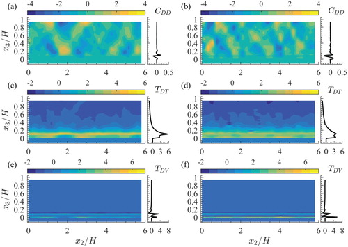
Figure 9. Spatial distributions of the energy-converting terms of the TKE balance of Eq. (5(5) $\begin{array}{rl}& \underset{\left(1\right):C_{TD}}{\underbrace{\frac{1}{2}\frac{\mathrm{\partial }}{\mathrm{\partial }{x}_j}({\phi }_{Vm}⟨{\phi }_T\overline{u_i^{\mathrm{\prime }}{u}_i^{\mathrm{\prime }}}⟩⟨{\overline{u}}_j⟩)}}\\ & =-\underset{\left(2\right):-P_{TT}}{\underbrace{{\phi }_{Vm}⟨{\phi }_T\overline{u_i^{\mathrm{\prime }}{u}_j^{\mathrm{\prime }}}⟩\frac{\mathrm{\partial }⟨{\overline{u}}_i⟩}{\mathrm{\partial }{x}_j}}}-\underset{\left(3\right):-P_{TF}}{\underbrace{{\phi }_{Vm}⟨{\phi }_T\overline{u_i^{\mathrm{\prime }}{u}_j^{\mathrm{\prime }}}\frac{\mathrm{\partial }{\tilde{\overline{u}}}_i}{\mathrm{\partial }{x}_j}⟩}}\\ & -\underset{\left(4\right):-T_{TF}}{\underbrace{\frac{1}{2}\frac{\mathrm{\partial }}{\mathrm{\partial }{x}_j}({\phi }_{Vm}⟨{\phi }_T\overline{u_i^{\mathrm{\prime }}{u}_i^{\mathrm{\prime }}}{\tilde{\overline{u}}}_j⟩)}}-\underset{\left(5\right):-T_{TT}}{\underbrace{\frac{1}{2}\frac{\mathrm{\partial }}{\mathrm{\partial }{x}_j}({\phi }_{Vm}⟨{\phi }_T\overline{u_i^{\mathrm{\prime }}{u}_i^{\mathrm{\prime }}{u}_j^{\mathrm{\prime }}}⟩)}}\\ & -\underset{\left(6\right):-T_{TP}}{\underbrace{\frac{1}{{\rho }_f}\frac{\mathrm{\partial }}{\mathrm{\partial }{x}_i}({\phi }_{Vm}⟨{\phi }_T\overline{u_i^{\mathrm{\prime }}{p}^{\mathrm{\prime }}}⟩)}}+\underset{\left(7\right):T_{TV}}{\underbrace{{\nu }_f\frac{\mathrm{\partial }}{\mathrm{\partial }{x}_j}\left({\phi }_{Vm}⟨{\phi }_T\overline{u_i^{\mathrm{\prime }}\frac{\mathrm{\partial }{u}_i^{\mathrm{\prime }}}{\mathrm{\partial }{x}_j}}⟩\right)}}\\ & +\underset{\left(8\right):P_{TP}}{\underbrace{\frac{{\phi }_{Vm}}{{\rho }_f}⟨{\phi }_T\overline{p^{\mathrm{\prime }}\frac{\mathrm{\partial }{u}_i^{\mathrm{\prime }}}{\mathrm{\partial }{x}_i}}⟩}}-\underset{\left(9\right):-D_T}{\underbrace{{\nu }_f{\phi }_{Vm}⟨{\phi }_T\overline{\frac{\mathrm{\partial }{u}_i^{\mathrm{\prime }}}{\mathrm{\partial }{x}_j}\frac{\mathrm{\partial }{u}_i^{\mathrm{\prime }}}{\mathrm{\partial }{x}_j}}⟩}}\\ & +\underset{\left(10\right):{\Phi }_T}{\underbrace{\frac{1}{{\rho }_f{V}_0}{\overline{{\int }_{S_{int}}{u}_i^{\mathrm{\prime }}p{n}_i\mathrm{d}S}}^s-\frac{1}{V_0}{\overline{{\int }_{S_{int}}{\nu }_f{u}_i^{\mathrm{\prime }}\frac{\mathrm{\partial }{u}_i}{\mathrm{\partial }{x}_j}{n}_j\mathrm{d}S}}^s}}\end{array}$(5) ): turbulent production $P_{TT}$ (term 2) for scenarios HP (a) and LP (b); viscous dissipation $D_T$ (term 9) for scenarios HP (c) and LP (d). The values of the TKE budget terms are normalized on $f_1{U}_b$

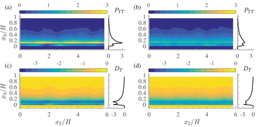
Figure 10. Spatial distributions of the transport terms of the TKE balance of Eq. (5(5) $\begin{array}{rl}& \underset{\left(1\right):C_{TD}}{\underbrace{\frac{1}{2}\frac{\mathrm{\partial }}{\mathrm{\partial }{x}_j}({\phi }_{Vm}⟨{\phi }_T\overline{u_i^{\mathrm{\prime }}{u}_i^{\mathrm{\prime }}}⟩⟨{\overline{u}}_j⟩)}}\\ & =-\underset{\left(2\right):-P_{TT}}{\underbrace{{\phi }_{Vm}⟨{\phi }_T\overline{u_i^{\mathrm{\prime }}{u}_j^{\mathrm{\prime }}}⟩\frac{\mathrm{\partial }⟨{\overline{u}}_i⟩}{\mathrm{\partial }{x}_j}}}-\underset{\left(3\right):-P_{TF}}{\underbrace{{\phi }_{Vm}⟨{\phi }_T\overline{u_i^{\mathrm{\prime }}{u}_j^{\mathrm{\prime }}}\frac{\mathrm{\partial }{\tilde{\overline{u}}}_i}{\mathrm{\partial }{x}_j}⟩}}\\ & -\underset{\left(4\right):-T_{TF}}{\underbrace{\frac{1}{2}\frac{\mathrm{\partial }}{\mathrm{\partial }{x}_j}({\phi }_{Vm}⟨{\phi }_T\overline{u_i^{\mathrm{\prime }}{u}_i^{\mathrm{\prime }}}{\tilde{\overline{u}}}_j⟩)}}-\underset{\left(5\right):-T_{TT}}{\underbrace{\frac{1}{2}\frac{\mathrm{\partial }}{\mathrm{\partial }{x}_j}({\phi }_{Vm}⟨{\phi }_T\overline{u_i^{\mathrm{\prime }}{u}_i^{\mathrm{\prime }}{u}_j^{\mathrm{\prime }}}⟩)}}\\ & -\underset{\left(6\right):-T_{TP}}{\underbrace{\frac{1}{{\rho }_f}\frac{\mathrm{\partial }}{\mathrm{\partial }{x}_i}({\phi }_{Vm}⟨{\phi }_T\overline{u_i^{\mathrm{\prime }}{p}^{\mathrm{\prime }}}⟩)}}+\underset{\left(7\right):T_{TV}}{\underbrace{{\nu }_f\frac{\mathrm{\partial }}{\mathrm{\partial }{x}_j}\left({\phi }_{Vm}⟨{\phi }_T\overline{u_i^{\mathrm{\prime }}\frac{\mathrm{\partial }{u}_i^{\mathrm{\prime }}}{\mathrm{\partial }{x}_j}}⟩\right)}}\\ & +\underset{\left(8\right):P_{TP}}{\underbrace{\frac{{\phi }_{Vm}}{{\rho }_f}⟨{\phi }_T\overline{p^{\mathrm{\prime }}\frac{\mathrm{\partial }{u}_i^{\mathrm{\prime }}}{\mathrm{\partial }{x}_i}}⟩}}-\underset{\left(9\right):-D_T}{\underbrace{{\nu }_f{\phi }_{Vm}⟨{\phi }_T\overline{\frac{\mathrm{\partial }{u}_i^{\mathrm{\prime }}}{\mathrm{\partial }{x}_j}\frac{\mathrm{\partial }{u}_i^{\mathrm{\prime }}}{\mathrm{\partial }{x}_j}}⟩}}\\ & +\underset{\left(10\right):{\Phi }_T}{\underbrace{\frac{1}{{\rho }_f{V}_0}{\overline{{\int }_{S_{int}}{u}_i^{\mathrm{\prime }}p{n}_i\mathrm{d}S}}^s-\frac{1}{V_0}{\overline{{\int }_{S_{int}}{\nu }_f{u}_i^{\mathrm{\prime }}\frac{\mathrm{\partial }{u}_i}{\mathrm{\partial }{x}_j}{n}_j\mathrm{d}S}}^s}}\end{array}$(5) ): mean convection $C_{TD}$ (term 1) for scenarios HP (a) and LP (b); turbulent convection $T_{TT}$ (term 5) for scenarios HP (c) and LP (d); pressure transport $T_{TP}$ (term 6) for scenarios HP (e) and LP (f); viscous transport $T_{TV}$ (term 7) for scenarios HP (g) and LP (h). The values of the TKE budget terms are normalized on $f_1{U}_b$

The data show that the bed configuration may visibly affect the shear TKE production $P_{TT}$ (term 2, Eq. 5(5) $\begin{array}{rl}& \underset{\left(1\right):C_{TD}}{\underbrace{\frac{1}{2}\frac{\mathrm{\partial }}{\mathrm{\partial }{x}_j}({\phi }_{Vm}⟨{\phi }_T\overline{u_i^{\mathrm{\prime }}{u}_i^{\mathrm{\prime }}}⟩⟨{\overline{u}}_j⟩)}}\\ & =-\underset{\left(2\right):-P_{TT}}{\underbrace{{\phi }_{Vm}⟨{\phi }_T\overline{u_i^{\mathrm{\prime }}{u}_j^{\mathrm{\prime }}}⟩\frac{\mathrm{\partial }⟨{\overline{u}}_i⟩}{\mathrm{\partial }{x}_j}}}-\underset{\left(3\right):-P_{TF}}{\underbrace{{\phi }_{Vm}⟨{\phi }_T\overline{u_i^{\mathrm{\prime }}{u}_j^{\mathrm{\prime }}}\frac{\mathrm{\partial }{\tilde{\overline{u}}}_i}{\mathrm{\partial }{x}_j}⟩}}\\ & -\underset{\left(4\right):-T_{TF}}{\underbrace{\frac{1}{2}\frac{\mathrm{\partial }}{\mathrm{\partial }{x}_j}({\phi }_{Vm}⟨{\phi }_T\overline{u_i^{\mathrm{\prime }}{u}_i^{\mathrm{\prime }}}{\tilde{\overline{u}}}_j⟩)}}-\underset{\left(5\right):-T_{TT}}{\underbrace{\frac{1}{2}\frac{\mathrm{\partial }}{\mathrm{\partial }{x}_j}({\phi }_{Vm}⟨{\phi }_T\overline{u_i^{\mathrm{\prime }}{u}_i^{\mathrm{\prime }}{u}_j^{\mathrm{\prime }}}⟩)}}\\ & -\underset{\left(6\right):-T_{TP}}{\underbrace{\frac{1}{{\rho }_f}\frac{\mathrm{\partial }}{\mathrm{\partial }{x}_i}({\phi }_{Vm}⟨{\phi }_T\overline{u_i^{\mathrm{\prime }}{p}^{\mathrm{\prime }}}⟩)}}+\underset{\left(7\right):T_{TV}}{\underbrace{{\nu }_f\frac{\mathrm{\partial }}{\mathrm{\partial }{x}_j}\left({\phi }_{Vm}⟨{\phi }_T\overline{u_i^{\mathrm{\prime }}\frac{\mathrm{\partial }{u}_i^{\mathrm{\prime }}}{\mathrm{\partial }{x}_j}}⟩\right)}}\\ & +\underset{\left(8\right):P_{TP}}{\underbrace{\frac{{\phi }_{Vm}}{{\rho }_f}⟨{\phi }_T\overline{p^{\mathrm{\prime }}\frac{\mathrm{\partial }{u}_i^{\mathrm{\prime }}}{\mathrm{\partial }{x}_i}}⟩}}-\underset{\left(9\right):-D_T}{\underbrace{{\nu }_f{\phi }_{Vm}⟨{\phi }_T\overline{\frac{\mathrm{\partial }{u}_i^{\mathrm{\prime }}}{\mathrm{\partial }{x}_j}\frac{\mathrm{\partial }{u}_i^{\mathrm{\prime }}}{\mathrm{\partial }{x}_j}}⟩}}\\ & +\underset{\left(10\right):{\Phi }_T}{\underbrace{\frac{1}{{\rho }_f{V}_0}{\overline{{\int }_{S_{int}}{u}_i^{\mathrm{\prime }}p{n}_i\mathrm{d}S}}^s-\frac{1}{V_0}{\overline{{\int }_{S_{int}}{\nu }_f{u}_i^{\mathrm{\prime }}\frac{\mathrm{\partial }{u}_i}{\mathrm{\partial }{x}_j}{n}_j\mathrm{d}S}}^s}}\end{array}$(5) ). The formation of stable particle clusters in scenario HP leads to the local increase of the magnitude of $P_{TT}$ at $x_3\approx 0.1H$ in the areas surrounding the clusters from both sides (Fig. 9a). At the location of the stable clusters, TKE production is decreased and this is particularly noticeable at $x_2\approx 2H$. For scenario LP, the magnitude of the production term $P_{TT}$ is also locally decreased at the locations of small-scale unstable clusters, i.e. at $x_2\approx 0.26H$, $2H$, 3.8H, 5.5H, for $0<x_3<0.2H$ (Fig. 9b).

The local estimates of the double-mean convective transport of TKE (term 1, $C_{TD}$; Fig. 10a and b) are highly heterogeneous within $0<x_3<0.4H$, changing from negative to positive values. The dimensions of anomalous patches of convective transport vary depending on their locations across the flow and in the vertical direction. Within $0<x_3<0.15H$, the height of these regions is approximately 0.1H for both scenarios, while for $x_3>0.15H$ their height becomes larger. Their width is larger close to the particle clusters, particularly close to the stable cluster at $x_2\approx 2H$ for scenario HP, and smaller away from the clusters. Similar patches are also noted in the local estimates of the convective terms in the balances of double-averaged momentum (fig. 10 in Vowinckel et al., 2017a) as well as in DMKE and FKE balances (Figs 4a, b and 7a, b). Note that the effects of the secondary currents on flow structure and momentum transport for HP and LP scenarios are discussed in Vowinckel et al. (2017b) who highlight their role in formation of the convection patches.

Turbulent convection (term 5, $T_{TT}$; Fig. 10c) is significant but in scenario HP it varies little in the spanwise direction. Apart from few distinct spots with high and low values, turbulent convection $T_{TT}$ is lower in scenario LP than for HP (Fig. 10c and d). The difference in the magnitudes of the pressure transport (term 6, $T_{TP}$; Fig. 10e and f) between the two scenarios appears to be significant, being higher for scenario LP where its spatial distribution is highly heterogeneous in the spanwise direction (Fig. 10f). No clear transfer pattern can be noted in Fig. 10f except for a thin layer with positive values at $x_3\approx -0.08H$ that extends from $x_2\approx 0.5H$ to the right edge of the domain. Viscous transport (term 7, $T_{TV}$; Fig. 10g) is clearly affected by bed configuration for scenario HP, as higher values are observed close to the levels $x_3=0$ and $x_3=0.1H$, on the left and right sides of the stable cluster at $x_2\approx 2H$. In scenario LP, viscous transport $T_{TV}$ becomes significant close to the level $x_3=0$ only, being fairly homogeneous in the spanwise direction.

The effect of the bed geometry can be also noted in the local estimates of viscous dissipation (term 9, $D_T$; Fig. 9c and d). For scenario HP, viscous dissipation $D_T$ is enhanced on the top of stable clusters (most significant at $x_2\approx 2H$, Fig. 9c). For scenario LP, the local viscous dissipation is less heterogeneous in the spanwise direction (Fig. 9d).

4. Discussion

This paper has presented an application of the double-averaging methodology to study the interactions between the flow and a rough bed composed of a layer of mobile particles moving above a layer of fixed particles. Equations for the double-averaged kinetic energy budgets have been applied for flows over beds composed by particles of the same size and shape; however, the equations can be used for flows over beds composed by roughness elements of different sizes and shapes. High-resolution data obtained by direct numerical simulations enabled the assessment of most terms in the DMKE, FKE and spatially averaged TKE budgets. The simulations have been conducted at the friction Reynolds number ${\text{R}}_{\text{τ}}=177$ and the roughness Reynolds number ${\mathsf{D}}^{+}=19.2$, for flows of intermediate submergence, i.e. at H=9D. The assessment of the terms involved in the recently proposed equations for the DMKE, FKE and TKE for mobile-bed flows provided information on the key energy exchanges and can reveal dominant mechanisms involved in flows with active bedload (e.g. energy fluxes between double-mean, form-induced, turbulent energy balances and particle motion).

Figures 4a, b and 7a, b characterize the convection of the DMKE and FKE, respectively. As the figures suggest, near the bed where mean velocity is significantly lower compared to the upper flow layers, the heterogeneity of the time-averaged velocity field ${\overline{u}}_i$ can be captured well by the FKE balance. In the upper flow region where the time porosity is $⟨{\phi }_T⟩\approx 1$, the heterogeneity of the time-averaged velocity field ${\overline{u}}_i$ is significantly weaker and the changes in the total mean energy $\frac{1}{2}{\overline{u}}_i{\overline{u}}_i$ balance (which is a sum of DMKE and FKE balances) can be adequately captured by the DMKE balance alone.

Considering local spatial averages, it is found that the secondary currents effects are visible in the distributions of the mean convective terms $C_{DD}$, $C_{FD}$ and $C_{TD}$ in the budgets of double-mean, form-induced and spatially averaged TKE. Bed morphology clearly affects energy generation, transport and dissipation mechanisms. For the HP scenario, well-developed bed forms stimulate strong form-induced and spatially averaged turbulent stresses that drive the energy transport and conversion mechanisms. For the LP scenario, particle mobility is increased, bed forms are less significant, and turbulent and form-induced stresses are weaker; as a result the work of pressure and viscous stresses control the energy transport and conversion.

The initial energy is supplied to the double-mean budget through work of the volume force $f_1$ that imitates the effect of gravity in the DNS (term 3, $G_D$ in Eq. 3(3) $\begin{array}{rl}& \underset{\left(1\right):C_{DD}}{\underbrace{\frac{1}{2}\frac{\mathrm{\partial }}{\mathrm{\partial }{x}_j}({\phi }_{VT}⟨{\overline{u}}_i⟩⟨{\overline{u}}_i⟩⟨{\overline{u}}_j⟩)}}+\underset{\left(2\right):C_{DM}}{\underbrace{\frac{\mathrm{\partial }}{\mathrm{\partial }{x}_j}({\phi }_{Vm}⟨{\phi }_T{\tilde{\overline{u}}}_i⟩⟨{\overline{u}}_i⟩⟨{\overline{u}}_j⟩)}}\\ & =\underset{\left(3\right):G_D}{\underbrace{{\phi }_{VT}⟨{\overline{u}}_1⟩f_1}}-\underset{\left(4\right):-T_{DT}}{\underbrace{\frac{\mathrm{\partial }}{\mathrm{\partial }{x}_j}({\phi }_{Vm}⟨{\phi }_T\overline{u_i^{\mathrm{\prime }}{u}_j^{\mathrm{\prime }}}⟩⟨{\overline{u}}_i⟩)}}\\ & -\underset{\left(5\right):-T_{DF}}{\underbrace{\frac{\mathrm{\partial }}{\mathrm{\partial }{x}_j}({\phi }_{Vm}⟨{\phi }_T{\tilde{\overline{u}}}_i{\tilde{\overline{u}}}_j⟩⟨{\overline{u}}_i⟩)}}-\underset{\left(6\right):-T_{DM}}{\underbrace{\frac{1}{2}\frac{\mathrm{\partial }}{\mathrm{\partial }{x}_j}({\phi }_{Vm}⟨{\phi }_T{\tilde{\overline{u}}}_j⟩⟨{\overline{u}}_i⟩⟨{\overline{u}}_i⟩)}}\\ & -\underset{\left(7\right):-T_{DP}}{\underbrace{\frac{1}{{\rho }_f}\frac{\mathrm{\partial }}{\mathrm{\partial }{x}_i}({\phi }_{Vm}⟨{\phi }_T\overline{p}⟩⟨{\overline{u}}_i⟩)}}+\underset{\left(8\right):T_{DV}}{\underbrace{{\nu }_f\frac{\mathrm{\partial }}{\mathrm{\partial }{x}_j}({\phi }_{Vm}⟨{\phi }_T\overline{\frac{\mathrm{\partial }{u}_i}{\mathrm{\partial }{x}_j}}⟩⟨{\overline{u}}_i⟩)}}\\ & +\underset{\left(9\right):P_{DT}}{\underbrace{{\phi }_{Vm}⟨{\phi }_T\overline{u_i^{\mathrm{\prime }}{u}_j^{\mathrm{\prime }}}⟩\frac{\mathrm{\partial }⟨{\overline{u}}_i⟩}{\mathrm{\partial }{x}_j}}}+\underset{\left(10\right):P_{DF}}{\underbrace{{\phi }_{Vm}⟨{\phi }_T{\tilde{\overline{u}}}_i{\tilde{\overline{u}}}_j⟩\frac{\mathrm{\partial }⟨{\overline{u}}_i⟩}{\mathrm{\partial }{x}_j}}}\\ & +\underset{\left(11\right):P_{DM}}{\underbrace{{\phi }_{Vm}⟨{\phi }_T{\tilde{\overline{u}}}_i⟩⟨{\overline{u}}_j⟩\frac{\mathrm{\partial }⟨{\overline{u}}_i⟩}{\mathrm{\partial }{x}_j}}}\\ & +\underset{\left(12\right):P_{DP}}{\underbrace{\frac{{\phi }_{Vm}⟨{\phi }_T\overline{p}⟩}{{\rho }_f}\frac{\mathrm{\partial }⟨{\overline{u}}_i⟩}{\mathrm{\partial }{x}_i}}}-\underset{\left(13\right):-D_D}{\underbrace{{\nu }_f{\phi }_{Vm}⟨{\phi }_T\overline{\frac{\mathrm{\partial }{u}_i}{\mathrm{\partial }{x}_j}}⟩\frac{\mathrm{\partial }⟨{\overline{u}}_i⟩}{\mathrm{\partial }{x}_j}}}\\ & +\underset{\left(14\right):{\Phi }_D}{\underbrace{\frac{⟨{\overline{u}}_i⟩}{{\rho }_f{V}_0}{\overline{{\int }_{S_{int}}p{n}_i\mathrm{d}S}}^s-\frac{⟨{\overline{u}}_i⟩}{V_0}{\overline{{\int }_{S_{int}}{\nu }_f\frac{\mathrm{\partial }{u}_i}{\mathrm{\partial }{x}_j}{n}_j\mathrm{d}S}}^s}}\end{array}$(3) ). This energy term does not depend noticeably on bed mobility for the scenarios examined, with bed morphology effect resulting in small variations of the term's magnitude in the near-wall region. However, particle mobility seems to affect the energy supply to the FKE and TKE budgets from the DMKE budget. The energy to the form-induced flow field is provided via (i) work of form-induced stresses on double-mean strain rate (term 3, $P_{FF}$ in Eq. 4(4) $\begin{array}{rl}& \underset{\left(1\right):C_{FD}}{\underbrace{\frac{1}{2}\frac{\mathrm{\partial }}{\mathrm{\partial }{x}_j}({\phi }_{Vm}⟨{\phi }_T{\tilde{\overline{u}}}_i{\tilde{\overline{u}}}_i⟩⟨{\overline{u}}_j⟩)}}\\ & =\underset{\left(2\right):G_F}{\underbrace{{\phi }_{Vm}⟨{\phi }_T{\tilde{\overline{u}}}_1⟩f_1}}-\underset{\left(3\right):-P_{FF}}{\underbrace{{\phi }_{Vm}⟨{\phi }_T{\tilde{\overline{u}}}_i{\tilde{\overline{u}}}_j⟩\frac{⟨{\overline{u}}_i⟩}{\mathrm{\partial }{x}_j}}}\\ & -\underset{\left(4\right):-P_{FM}}{\underbrace{{\phi }_{Vm}⟨{\phi }_T{\tilde{\overline{u}}}_i⟩⟨{\overline{u}}_j⟩\frac{\mathrm{\partial }⟨{\overline{u}}_i⟩}{\mathrm{\partial }{x}_j}}}-\underset{\left(5\right):-T_{FF}}{\underbrace{\frac{1}{2}\frac{\mathrm{\partial }}{\mathrm{\partial }{x}_j}({\phi }_{Vm}⟨{\phi }_T{\tilde{\overline{u}}}_i{\tilde{\overline{u}}}_i{\tilde{\overline{u}}}_j⟩)}}\\ & -\underset{\left(6\right):-T_{FF}}{\underbrace{\frac{\mathrm{\partial }}{\mathrm{\partial }{x}_j}({\phi }_{Vm}⟨{\phi }_T\overline{u_i^{\mathrm{\prime }}{u}_j^{\mathrm{\prime }}}{\tilde{\overline{u}}}_i⟩)}}-\underset{\left(7\right):-T_{FP}}{\underbrace{\frac{1}{{\rho }_f}\frac{\mathrm{\partial }}{\mathrm{\partial }{x}_i}({\phi }_{Vm}⟨{\phi }_T\overline{p}{\tilde{\overline{u}}}_i⟩)}}\\ & +\underset{\left(8\right):T_{FV}}{\underbrace{{\nu }_f\frac{\mathrm{\partial }}{\mathrm{\partial }{x}_j}({\phi }_{Vm}⟨{\phi }_T\overline{\frac{\mathrm{\partial }{u}_i}{\mathrm{\partial }{x}_j}}{\tilde{\overline{u}}}_i⟩)}}+\underset{\left(9\right):P_{FT}}{\underbrace{{\phi }_{Vm}⟨{\phi }_T\overline{u_i^{\mathrm{\prime }}{u}_j^{\mathrm{\prime }}}\frac{\mathrm{\partial }{\tilde{\overline{u}}}_i}{\mathrm{\partial }{x}_j}⟩}}\\ & +\underset{\left(10\right):P_{FP}}{\underbrace{\frac{{\phi }_{Vm}}{{\rho }_f}⟨{\phi }_T\overline{p}\frac{\mathrm{\partial }{\tilde{\overline{u}}}_i}{\mathrm{\partial }{x}_i}⟩}}-\underset{\left(11\right):-D_F}{\underbrace{{\nu }_f{\phi }_{Vm}⟨{\phi }_T\overline{\frac{\mathrm{\partial }{u}_i}{\mathrm{\partial }{x}_j}}\frac{\mathrm{\partial }{\tilde{\overline{u}}}_i}{\mathrm{\partial }{x}_j}⟩}}\\ & +\underset{\left(12\right):{\Phi }_F}{\underbrace{\frac{1}{{\rho }_f{V}_0}{\overline{{\int }_{S_{int}}{\tilde{\overline{u}}}_{i}p{n}_i\mathrm{d}S}}^s-\frac{1}{V_0}{\overline{{\int }_{S_{int}}{\nu }_f{\tilde{\overline{u}}}_i\frac{\mathrm{\partial }{u}_i}{\mathrm{\partial }{x}_j}{n}_j\mathrm{d}S}}^s}}\end{array}$(4) ) and (ii) work of viscous stresses and pressure on the interfacial surfaces (term 12, ${\Phi }_F$ in Eq. 4(4) $\begin{array}{rl}& \underset{\left(1\right):C_{FD}}{\underbrace{\frac{1}{2}\frac{\mathrm{\partial }}{\mathrm{\partial }{x}_j}({\phi }_{Vm}⟨{\phi }_T{\tilde{\overline{u}}}_i{\tilde{\overline{u}}}_i⟩⟨{\overline{u}}_j⟩)}}\\ & =\underset{\left(2\right):G_F}{\underbrace{{\phi }_{Vm}⟨{\phi }_T{\tilde{\overline{u}}}_1⟩f_1}}-\underset{\left(3\right):-P_{FF}}{\underbrace{{\phi }_{Vm}⟨{\phi }_T{\tilde{\overline{u}}}_i{\tilde{\overline{u}}}_j⟩\frac{⟨{\overline{u}}_i⟩}{\mathrm{\partial }{x}_j}}}\\ & -\underset{\left(4\right):-P_{FM}}{\underbrace{{\phi }_{Vm}⟨{\phi }_T{\tilde{\overline{u}}}_i⟩⟨{\overline{u}}_j⟩\frac{\mathrm{\partial }⟨{\overline{u}}_i⟩}{\mathrm{\partial }{x}_j}}}-\underset{\left(5\right):-T_{FF}}{\underbrace{\frac{1}{2}\frac{\mathrm{\partial }}{\mathrm{\partial }{x}_j}({\phi }_{Vm}⟨{\phi }_T{\tilde{\overline{u}}}_i{\tilde{\overline{u}}}_i{\tilde{\overline{u}}}_j⟩)}}\\ & -\underset{\left(6\right):-T_{FF}}{\underbrace{\frac{\mathrm{\partial }}{\mathrm{\partial }{x}_j}({\phi }_{Vm}⟨{\phi }_T\overline{u_i^{\mathrm{\prime }}{u}_j^{\mathrm{\prime }}}{\tilde{\overline{u}}}_i⟩)}}-\underset{\left(7\right):-T_{FP}}{\underbrace{\frac{1}{{\rho }_f}\frac{\mathrm{\partial }}{\mathrm{\partial }{x}_i}({\phi }_{Vm}⟨{\phi }_T\overline{p}{\tilde{\overline{u}}}_i⟩)}}\\ & +\underset{\left(8\right):T_{FV}}{\underbrace{{\nu }_f\frac{\mathrm{\partial }}{\mathrm{\partial }{x}_j}({\phi }_{Vm}⟨{\phi }_T\overline{\frac{\mathrm{\partial }{u}_i}{\mathrm{\partial }{x}_j}}{\tilde{\overline{u}}}_i⟩)}}+\underset{\left(9\right):P_{FT}}{\underbrace{{\phi }_{Vm}⟨{\phi }_T\overline{u_i^{\mathrm{\prime }}{u}_j^{\mathrm{\prime }}}\frac{\mathrm{\partial }{\tilde{\overline{u}}}_i}{\mathrm{\partial }{x}_j}⟩}}\\ & +\underset{\left(10\right):P_{FP}}{\underbrace{\frac{{\phi }_{Vm}}{{\rho }_f}⟨{\phi }_T\overline{p}\frac{\mathrm{\partial }{\tilde{\overline{u}}}_i}{\mathrm{\partial }{x}_i}⟩}}-\underset{\left(11\right):-D_F}{\underbrace{{\nu }_f{\phi }_{Vm}⟨{\phi }_T\overline{\frac{\mathrm{\partial }{u}_i}{\mathrm{\partial }{x}_j}}\frac{\mathrm{\partial }{\tilde{\overline{u}}}_i}{\mathrm{\partial }{x}_j}⟩}}\\ & +\underset{\left(12\right):{\Phi }_F}{\underbrace{\frac{1}{{\rho }_f{V}_0}{\overline{{\int }_{S_{int}}{\tilde{\overline{u}}}_{i}p{n}_i\mathrm{d}S}}^s-\frac{1}{V_0}{\overline{{\int }_{S_{int}}{\nu }_f{\tilde{\overline{u}}}_i\frac{\mathrm{\partial }{u}_i}{\mathrm{\partial }{x}_j}{n}_j\mathrm{d}S}}^s}}\end{array}$(4) ). The first mechanism brings energy to FKE from the double-mean flow directly, while the second mechanism transfers energy from the double-mean flow indirectly by the particle motion action. Particle mobility appears to affect the magnitude of both mechanisms, as the enhanced motion of mobile particles prevents the formation of stable bed features that leads to weakening of the first mechanism (as shear form-induced stresses become weaker) and the strengthening of the second mechanism.

The energy supply to the turbulent flow field comes from (i) the double-mean flow through the work of the Reynolds stresses on the double-mean strain rate (term 2, $P_{TT}$ in Eq. 5(5) $\begin{array}{rl}& \underset{\left(1\right):C_{TD}}{\underbrace{\frac{1}{2}\frac{\mathrm{\partial }}{\mathrm{\partial }{x}_j}({\phi }_{Vm}⟨{\phi }_T\overline{u_i^{\mathrm{\prime }}{u}_i^{\mathrm{\prime }}}⟩⟨{\overline{u}}_j⟩)}}\\ & =-\underset{\left(2\right):-P_{TT}}{\underbrace{{\phi }_{Vm}⟨{\phi }_T\overline{u_i^{\mathrm{\prime }}{u}_j^{\mathrm{\prime }}}⟩\frac{\mathrm{\partial }⟨{\overline{u}}_i⟩}{\mathrm{\partial }{x}_j}}}-\underset{\left(3\right):-P_{TF}}{\underbrace{{\phi }_{Vm}⟨{\phi }_T\overline{u_i^{\mathrm{\prime }}{u}_j^{\mathrm{\prime }}}\frac{\mathrm{\partial }{\tilde{\overline{u}}}_i}{\mathrm{\partial }{x}_j}⟩}}\\ & -\underset{\left(4\right):-T_{TF}}{\underbrace{\frac{1}{2}\frac{\mathrm{\partial }}{\mathrm{\partial }{x}_j}({\phi }_{Vm}⟨{\phi }_T\overline{u_i^{\mathrm{\prime }}{u}_i^{\mathrm{\prime }}}{\tilde{\overline{u}}}_j⟩)}}-\underset{\left(5\right):-T_{TT}}{\underbrace{\frac{1}{2}\frac{\mathrm{\partial }}{\mathrm{\partial }{x}_j}({\phi }_{Vm}⟨{\phi }_T\overline{u_i^{\mathrm{\prime }}{u}_i^{\mathrm{\prime }}{u}_j^{\mathrm{\prime }}}⟩)}}\\ & -\underset{\left(6\right):-T_{TP}}{\underbrace{\frac{1}{{\rho }_f}\frac{\mathrm{\partial }}{\mathrm{\partial }{x}_i}({\phi }_{Vm}⟨{\phi }_T\overline{u_i^{\mathrm{\prime }}{p}^{\mathrm{\prime }}}⟩)}}+\underset{\left(7\right):T_{TV}}{\underbrace{{\nu }_f\frac{\mathrm{\partial }}{\mathrm{\partial }{x}_j}\left({\phi }_{Vm}⟨{\phi }_T\overline{u_i^{\mathrm{\prime }}\frac{\mathrm{\partial }{u}_i^{\mathrm{\prime }}}{\mathrm{\partial }{x}_j}}⟩\right)}}\\ & +\underset{\left(8\right):P_{TP}}{\underbrace{\frac{{\phi }_{Vm}}{{\rho }_f}⟨{\phi }_T\overline{p^{\mathrm{\prime }}\frac{\mathrm{\partial }{u}_i^{\mathrm{\prime }}}{\mathrm{\partial }{x}_i}}⟩}}-\underset{\left(9\right):-D_T}{\underbrace{{\nu }_f{\phi }_{Vm}⟨{\phi }_T\overline{\frac{\mathrm{\partial }{u}_i^{\mathrm{\prime }}}{\mathrm{\partial }{x}_j}\frac{\mathrm{\partial }{u}_i^{\mathrm{\prime }}}{\mathrm{\partial }{x}_j}}⟩}}\\ & +\underset{\left(10\right):{\Phi }_T}{\underbrace{\frac{1}{{\rho }_f{V}_0}{\overline{{\int }_{S_{int}}{u}_i^{\mathrm{\prime }}p{n}_i\mathrm{d}S}}^s-\frac{1}{V_0}{\overline{{\int }_{S_{int}}{\nu }_f{u}_i^{\mathrm{\prime }}\frac{\mathrm{\partial }{u}_i}{\mathrm{\partial }{x}_j}{n}_j\mathrm{d}S}}^s}}\end{array}$(5) ), and (ii) the motion of mobile particles for $x_3>0$ through the work of hydrodynamic stresses on the interfacial surface (term 10, ${\Phi }_T$ in Eq. 5(5) $\begin{array}{rl}& \underset{\left(1\right):C_{TD}}{\underbrace{\frac{1}{2}\frac{\mathrm{\partial }}{\mathrm{\partial }{x}_j}({\phi }_{Vm}⟨{\phi }_T\overline{u_i^{\mathrm{\prime }}{u}_i^{\mathrm{\prime }}}⟩⟨{\overline{u}}_j⟩)}}\\ & =-\underset{\left(2\right):-P_{TT}}{\underbrace{{\phi }_{Vm}⟨{\phi }_T\overline{u_i^{\mathrm{\prime }}{u}_j^{\mathrm{\prime }}}⟩\frac{\mathrm{\partial }⟨{\overline{u}}_i⟩}{\mathrm{\partial }{x}_j}}}-\underset{\left(3\right):-P_{TF}}{\underbrace{{\phi }_{Vm}⟨{\phi }_T\overline{u_i^{\mathrm{\prime }}{u}_j^{\mathrm{\prime }}}\frac{\mathrm{\partial }{\tilde{\overline{u}}}_i}{\mathrm{\partial }{x}_j}⟩}}\\ & -\underset{\left(4\right):-T_{TF}}{\underbrace{\frac{1}{2}\frac{\mathrm{\partial }}{\mathrm{\partial }{x}_j}({\phi }_{Vm}⟨{\phi }_T\overline{u_i^{\mathrm{\prime }}{u}_i^{\mathrm{\prime }}}{\tilde{\overline{u}}}_j⟩)}}-\underset{\left(5\right):-T_{TT}}{\underbrace{\frac{1}{2}\frac{\mathrm{\partial }}{\mathrm{\partial }{x}_j}({\phi }_{Vm}⟨{\phi }_T\overline{u_i^{\mathrm{\prime }}{u}_i^{\mathrm{\prime }}{u}_j^{\mathrm{\prime }}}⟩)}}\\ & -\underset{\left(6\right):-T_{TP}}{\underbrace{\frac{1}{{\rho }_f}\frac{\mathrm{\partial }}{\mathrm{\partial }{x}_i}({\phi }_{Vm}⟨{\phi }_T\overline{u_i^{\mathrm{\prime }}{p}^{\mathrm{\prime }}}⟩)}}+\underset{\left(7\right):T_{TV}}{\underbrace{{\nu }_f\frac{\mathrm{\partial }}{\mathrm{\partial }{x}_j}\left({\phi }_{Vm}⟨{\phi }_T\overline{u_i^{\mathrm{\prime }}\frac{\mathrm{\partial }{u}_i^{\mathrm{\prime }}}{\mathrm{\partial }{x}_j}}⟩\right)}}\\ & +\underset{\left(8\right):P_{TP}}{\underbrace{\frac{{\phi }_{Vm}}{{\rho }_f}⟨{\phi }_T\overline{p^{\mathrm{\prime }}\frac{\mathrm{\partial }{u}_i^{\mathrm{\prime }}}{\mathrm{\partial }{x}_i}}⟩}}-\underset{\left(9\right):-D_T}{\underbrace{{\nu }_f{\phi }_{Vm}⟨{\phi }_T\overline{\frac{\mathrm{\partial }{u}_i^{\mathrm{\prime }}}{\mathrm{\partial }{x}_j}\frac{\mathrm{\partial }{u}_i^{\mathrm{\prime }}}{\mathrm{\partial }{x}_j}}⟩}}\\ & +\underset{\left(10\right):{\Phi }_T}{\underbrace{\frac{1}{{\rho }_f{V}_0}{\overline{{\int }_{S_{int}}{u}_i^{\mathrm{\prime }}p{n}_i\mathrm{d}S}}^s-\frac{1}{V_0}{\overline{{\int }_{S_{int}}{\nu }_f{u}_i^{\mathrm{\prime }}\frac{\mathrm{\partial }{u}_i}{\mathrm{\partial }{x}_j}{n}_j\mathrm{d}S}}^s}}\end{array}$(5) ). Our analysis suggests that that the moving particles receive the energy directly from the double-mean flow and then part of this energy is handed to turbulence either directly or through the FKE balance. It is interesting to compare this finding for bedload particles with quite different conventional picture of energy transfer in sediment-laden flows. Velikanov (1944) was first to propose the energy-based approach in sediment transport and developed the so called “gravitational theory of suspended sediment transport” (described in detail in Dey, 2014; Yalin, 1977). The key element of his theory was an assumption that particles are kept in suspension due to the energy supply from the mean flow. This assumption was challenged by Kolmogorov (1954) who argued that suspended particles receive energy from turbulence rather than from the mean flow. According to Kolmogorov's (1954) concept, the mean (time-averaged) flow gets energy from gravity and then mainly transfers it to turbulence (with a small amount converted directly to heat). Turbulent motions, in turn, supply energy to sediment particles to keep them in suspension, in contrast to Velikanov (1944) who assigned this role to the mean flow. Both Velikanov's (1944) and Kolmogorov's (1954) concepts assume that the particles are very small compared to turbulence scales while their concentration is very low (thus particle collisions are rare). These assumptions allowed constructing hydrodynamic equations by considering a continuum of fluid–sediment mixture. The work for suspension arises in their energy balance equations based on physical considerations rather than directly derived, as in our study. These concepts for suspended particles can be supplemented with physical considerations of Grishin (1982) for bedload particles; this author suggested that motions of near-bed particles are driven by the mean energy flow and that these particles provide some energy to turbulence. He concluded that the energy exchanges in “flow-suspended particles interactions” and in “flow-bedload interactions” act in opposite directions due to different nature of bedload and suspended particle motions. Grishin's (1982) concept finds strong support in our quantitative analysis.

DMKE is “dissipated” into FKE, TKE and heat as well as being transferred to the particle motion. FKE is “dissipated” into heat and TKE below the tops of the stable cluster formed in scenario HP and above the fixed-particles tops in scenario LP. In scenario HP, in the flow layer where stable clusters are formed, TKE is converted into the FKE. The conversion of TKE to FKE occurs in scenario LP too, but its magnitude is significantly lower. The work of the Reynolds stresses on the form-induced strain rate (term 3, $P_{TF}$ in Eq. 5(5) $\begin{array}{rl}& \underset{\left(1\right):C_{TD}}{\underbrace{\frac{1}{2}\frac{\mathrm{\partial }}{\mathrm{\partial }{x}_j}({\phi }_{Vm}⟨{\phi }_T\overline{u_i^{\mathrm{\prime }}{u}_i^{\mathrm{\prime }}}⟩⟨{\overline{u}}_j⟩)}}\\ & =-\underset{\left(2\right):-P_{TT}}{\underbrace{{\phi }_{Vm}⟨{\phi }_T\overline{u_i^{\mathrm{\prime }}{u}_j^{\mathrm{\prime }}}⟩\frac{\mathrm{\partial }⟨{\overline{u}}_i⟩}{\mathrm{\partial }{x}_j}}}-\underset{\left(3\right):-P_{TF}}{\underbrace{{\phi }_{Vm}⟨{\phi }_T\overline{u_i^{\mathrm{\prime }}{u}_j^{\mathrm{\prime }}}\frac{\mathrm{\partial }{\tilde{\overline{u}}}_i}{\mathrm{\partial }{x}_j}⟩}}\\ & -\underset{\left(4\right):-T_{TF}}{\underbrace{\frac{1}{2}\frac{\mathrm{\partial }}{\mathrm{\partial }{x}_j}({\phi }_{Vm}⟨{\phi }_T\overline{u_i^{\mathrm{\prime }}{u}_i^{\mathrm{\prime }}}{\tilde{\overline{u}}}_j⟩)}}-\underset{\left(5\right):-T_{TT}}{\underbrace{\frac{1}{2}\frac{\mathrm{\partial }}{\mathrm{\partial }{x}_j}({\phi }_{Vm}⟨{\phi }_T\overline{u_i^{\mathrm{\prime }}{u}_i^{\mathrm{\prime }}{u}_j^{\mathrm{\prime }}}⟩)}}\\ & -\underset{\left(6\right):-T_{TP}}{\underbrace{\frac{1}{{\rho }_f}\frac{\mathrm{\partial }}{\mathrm{\partial }{x}_i}({\phi }_{Vm}⟨{\phi }_T\overline{u_i^{\mathrm{\prime }}{p}^{\mathrm{\prime }}}⟩)}}+\underset{\left(7\right):T_{TV}}{\underbrace{{\nu }_f\frac{\mathrm{\partial }}{\mathrm{\partial }{x}_j}\left({\phi }_{Vm}⟨{\phi }_T\overline{u_i^{\mathrm{\prime }}\frac{\mathrm{\partial }{u}_i^{\mathrm{\prime }}}{\mathrm{\partial }{x}_j}}⟩\right)}}\\ & +\underset{\left(8\right):P_{TP}}{\underbrace{\frac{{\phi }_{Vm}}{{\rho }_f}⟨{\phi }_T\overline{p^{\mathrm{\prime }}\frac{\mathrm{\partial }{u}_i^{\mathrm{\prime }}}{\mathrm{\partial }{x}_i}}⟩}}-\underset{\left(9\right):-D_T}{\underbrace{{\nu }_f{\phi }_{Vm}⟨{\phi }_T\overline{\frac{\mathrm{\partial }{u}_i^{\mathrm{\prime }}}{\mathrm{\partial }{x}_j}\frac{\mathrm{\partial }{u}_i^{\mathrm{\prime }}}{\mathrm{\partial }{x}_j}}⟩}}\\ & +\underset{\left(10\right):{\Phi }_T}{\underbrace{\frac{1}{{\rho }_f{V}_0}{\overline{{\int }_{S_{int}}{u}_i^{\mathrm{\prime }}p{n}_i\mathrm{d}S}}^s-\frac{1}{V_0}{\overline{{\int }_{S_{int}}{\nu }_f{u}_i^{\mathrm{\prime }}\frac{\mathrm{\partial }{u}_i}{\mathrm{\partial }{x}_j}{n}_j\mathrm{d}S}}^s}}\end{array}$(5) ) has insignificant effect on the TKE balance. This energy supply to the TKE budget is negligible compared to the energy provided by the double-mean flow due to the work of turbulent stress (term 2, $P_{TT}$ in Eq. 5(5) $\begin{array}{rl}& \underset{\left(1\right):C_{TD}}{\underbrace{\frac{1}{2}\frac{\mathrm{\partial }}{\mathrm{\partial }{x}_j}({\phi }_{Vm}⟨{\phi }_T\overline{u_i^{\mathrm{\prime }}{u}_i^{\mathrm{\prime }}}⟩⟨{\overline{u}}_j⟩)}}\\ & =-\underset{\left(2\right):-P_{TT}}{\underbrace{{\phi }_{Vm}⟨{\phi }_T\overline{u_i^{\mathrm{\prime }}{u}_j^{\mathrm{\prime }}}⟩\frac{\mathrm{\partial }⟨{\overline{u}}_i⟩}{\mathrm{\partial }{x}_j}}}-\underset{\left(3\right):-P_{TF}}{\underbrace{{\phi }_{Vm}⟨{\phi }_T\overline{u_i^{\mathrm{\prime }}{u}_j^{\mathrm{\prime }}}\frac{\mathrm{\partial }{\tilde{\overline{u}}}_i}{\mathrm{\partial }{x}_j}⟩}}\\ & -\underset{\left(4\right):-T_{TF}}{\underbrace{\frac{1}{2}\frac{\mathrm{\partial }}{\mathrm{\partial }{x}_j}({\phi }_{Vm}⟨{\phi }_T\overline{u_i^{\mathrm{\prime }}{u}_i^{\mathrm{\prime }}}{\tilde{\overline{u}}}_j⟩)}}-\underset{\left(5\right):-T_{TT}}{\underbrace{\frac{1}{2}\frac{\mathrm{\partial }}{\mathrm{\partial }{x}_j}({\phi }_{Vm}⟨{\phi }_T\overline{u_i^{\mathrm{\prime }}{u}_i^{\mathrm{\prime }}{u}_j^{\mathrm{\prime }}}⟩)}}\\ & -\underset{\left(6\right):-T_{TP}}{\underbrace{\frac{1}{{\rho }_f}\frac{\mathrm{\partial }}{\mathrm{\partial }{x}_i}({\phi }_{Vm}⟨{\phi }_T\overline{u_i^{\mathrm{\prime }}{p}^{\mathrm{\prime }}}⟩)}}+\underset{\left(7\right):T_{TV}}{\underbrace{{\nu }_f\frac{\mathrm{\partial }}{\mathrm{\partial }{x}_j}\left({\phi }_{Vm}⟨{\phi }_T\overline{u_i^{\mathrm{\prime }}\frac{\mathrm{\partial }{u}_i^{\mathrm{\prime }}}{\mathrm{\partial }{x}_j}}⟩\right)}}\\ & +\underset{\left(8\right):P_{TP}}{\underbrace{\frac{{\phi }_{Vm}}{{\rho }_f}⟨{\phi }_T\overline{p^{\mathrm{\prime }}\frac{\mathrm{\partial }{u}_i^{\mathrm{\prime }}}{\mathrm{\partial }{x}_i}}⟩}}-\underset{\left(9\right):-D_T}{\underbrace{{\nu }_f{\phi }_{Vm}⟨{\phi }_T\overline{\frac{\mathrm{\partial }{u}_i^{\mathrm{\prime }}}{\mathrm{\partial }{x}_j}\frac{\mathrm{\partial }{u}_i^{\mathrm{\prime }}}{\mathrm{\partial }{x}_j}}⟩}}\\ & +\underset{\left(10\right):{\Phi }_T}{\underbrace{\frac{1}{{\rho }_f{V}_0}{\overline{{\int }_{S_{int}}{u}_i^{\mathrm{\prime }}p{n}_i\mathrm{d}S}}^s-\frac{1}{V_0}{\overline{{\int }_{S_{int}}{\nu }_f{u}_i^{\mathrm{\prime }}\frac{\mathrm{\partial }{u}_i}{\mathrm{\partial }{x}_j}{n}_j\mathrm{d}S}}^s}}\end{array}$(5) ) and by particle motion (term 10, ${\Phi }_T$ in Eq. 5(5) $\begin{array}{rl}& \underset{\left(1\right):C_{TD}}{\underbrace{\frac{1}{2}\frac{\mathrm{\partial }}{\mathrm{\partial }{x}_j}({\phi }_{Vm}⟨{\phi }_T\overline{u_i^{\mathrm{\prime }}{u}_i^{\mathrm{\prime }}}⟩⟨{\overline{u}}_j⟩)}}\\ & =-\underset{\left(2\right):-P_{TT}}{\underbrace{{\phi }_{Vm}⟨{\phi }_T\overline{u_i^{\mathrm{\prime }}{u}_j^{\mathrm{\prime }}}⟩\frac{\mathrm{\partial }⟨{\overline{u}}_i⟩}{\mathrm{\partial }{x}_j}}}-\underset{\left(3\right):-P_{TF}}{\underbrace{{\phi }_{Vm}⟨{\phi }_T\overline{u_i^{\mathrm{\prime }}{u}_j^{\mathrm{\prime }}}\frac{\mathrm{\partial }{\tilde{\overline{u}}}_i}{\mathrm{\partial }{x}_j}⟩}}\\ & -\underset{\left(4\right):-T_{TF}}{\underbrace{\frac{1}{2}\frac{\mathrm{\partial }}{\mathrm{\partial }{x}_j}({\phi }_{Vm}⟨{\phi }_T\overline{u_i^{\mathrm{\prime }}{u}_i^{\mathrm{\prime }}}{\tilde{\overline{u}}}_j⟩)}}-\underset{\left(5\right):-T_{TT}}{\underbrace{\frac{1}{2}\frac{\mathrm{\partial }}{\mathrm{\partial }{x}_j}({\phi }_{Vm}⟨{\phi }_T\overline{u_i^{\mathrm{\prime }}{u}_i^{\mathrm{\prime }}{u}_j^{\mathrm{\prime }}}⟩)}}\\ & -\underset{\left(6\right):-T_{TP}}{\underbrace{\frac{1}{{\rho }_f}\frac{\mathrm{\partial }}{\mathrm{\partial }{x}_i}({\phi }_{Vm}⟨{\phi }_T\overline{u_i^{\mathrm{\prime }}{p}^{\mathrm{\prime }}}⟩)}}+\underset{\left(7\right):T_{TV}}{\underbrace{{\nu }_f\frac{\mathrm{\partial }}{\mathrm{\partial }{x}_j}\left({\phi }_{Vm}⟨{\phi }_T\overline{u_i^{\mathrm{\prime }}\frac{\mathrm{\partial }{u}_i^{\mathrm{\prime }}}{\mathrm{\partial }{x}_j}}⟩\right)}}\\ & +\underset{\left(8\right):P_{TP}}{\underbrace{\frac{{\phi }_{Vm}}{{\rho }_f}⟨{\phi }_T\overline{p^{\mathrm{\prime }}\frac{\mathrm{\partial }{u}_i^{\mathrm{\prime }}}{\mathrm{\partial }{x}_i}}⟩}}-\underset{\left(9\right):-D_T}{\underbrace{{\nu }_f{\phi }_{Vm}⟨{\phi }_T\overline{\frac{\mathrm{\partial }{u}_i^{\mathrm{\prime }}}{\mathrm{\partial }{x}_j}\frac{\mathrm{\partial }{u}_i^{\mathrm{\prime }}}{\mathrm{\partial }{x}_j}}⟩}}\\ & +\underset{\left(10\right):{\Phi }_T}{\underbrace{\frac{1}{{\rho }_f{V}_0}{\overline{{\int }_{S_{int}}{u}_i^{\mathrm{\prime }}p{n}_i\mathrm{d}S}}^s-\frac{1}{V_0}{\overline{{\int }_{S_{int}}{\nu }_f{u}_i^{\mathrm{\prime }}\frac{\mathrm{\partial }{u}_i}{\mathrm{\partial }{x}_j}{n}_j\mathrm{d}S}}^s}}\end{array}$(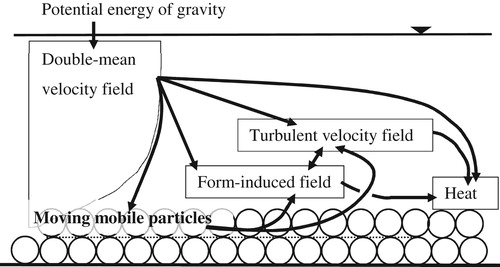5) ). TKE is dissipated into heat, particularly in the flow region around the particle clusters noted in Fig. 1. The energy transport mechanism is dominated by turbulent and viscous stresses. All the above provide some insights on the interactions of the double-mean, form-induced and turbulent velocity fields with particle motions highlighting the role of bed mobility in relation to the heterogeneity of the near-bed flow. Our findings on the energy fluxes in flows transporting bed particles are summarized in a schematic form in Fig. 11. Studies using data from mobile-boundary flows with higher Reynolds numbers are needed to further contribute to this subject.

Figure 11. Schematic representation of the energy fluxes (arrows) between double-mean flow, form-induced flow, turbulent flow and mobile bed in the particle transporting flows

5. Conclusions

Direct numerical simulations of turbulent open-channel flow over mobile granular beds were used to assess DMKE, FKE and TKE budgets and clarify turbulent energy production, spatial redistribution, and energy exchanges with the mean flow and moving sediment particles. The data represent two scenarios: one corresponding to near-critical condition at the bed and the other to a fully mobile granular bed. Three main conclusions can be drawn from the current study:

1. The work of the volume force ${\phi }_{VT}⟨{\overline{u}}_1⟩f_1$ supplies energy to the double-mean flow field. This external energy is found primarily in the flow region above the particle mobility zone, while below this region it gradually reduces to 0 at the tops of the fixed particles. Turbulent stresses remove energy from the upper flow region (approximately for $x_3>0.3H$) and transfer it to the near-wall region ($x_3<0.3H$). The DMKE transferred to the near-bed region is passed to the moving mobile particles, the turbulent and form-induced velocity fields as well as being dissipated to heat.

2. The double-mean velocity field and particle motion supply energy to the form-induced velocity field due to (i) shear FKE production and (ii) the work of the hydrodynamic stresses on the fluid–particle interface. Mechanism (i) is more effective than mechanism (ii) in scenario HP, due to the stronger shear form-induced stresses noted in this scenario. As form-induced stresses decrease and the fluid–particle interactions increase in scenario LP (compared to scenario HP), the interface-related mechanism (ii) becomes more significant than the shear production mechanism (i). As the Reynolds stresses are also weaker in scenario LP than in scenario HP (fig. 5 in Vowinckel et al., 2017b), the energy exchange between the balances of FKE and TKE is smaller for the former and occurs mainly as the “conversion” of FKE to TKE. In scenario HP, form-induced flow may also receive energy from turbulent flow at the tops of the clusters, while below this level FKE is “converted” into TKE. The development of stable particle clusters enhanced viscous dissipation at the clusters' tops in scenario HP. In the absence of stable clusters in scenario LP, viscous dissipation occurs mostly at the tops of the fixed particles.

3. The energy is supplied to turbulence from the double-mean flow directly due to shear turbulence production and indirectly through particle motion. Turbulent convection removes energy from the particle mobility zone and places it close to the tops of the fixed particles. Pressure effects are significantly stronger in scenario LP, as turbulent pressure transport transfers more energy below $x_3\approx 0$. The energy transferred above and near the tops of the fixed particles is then dissipated to heat due to the effect of viscosity.

These findings shed some light on the interactions between mean flow, turbulent flow and mobile particle motions and can be used for the construction and improvement of flow models for mobile-boundary conditions. Studies employing the double-averaged energy budgets to the analysis of flows with higher Reynolds number over mobile beds with more natural distributions of sediment shapes and/or size would be a valuable follow-up, once such data become available.

Notation

$C_D$	=	terms of convective transport of double-mean energy; combined with subscripts D or M to denote mean convective transport, or convective transport due to the velocity-time porosity correlation (m${}^2$ s${}^{-3}$)
$C_{FD}$	=	convective transport term of form-induced energy (m${}^2$ s${}^{-3}$)
$C_{TD}$	=	double-mean convective transport terms of turbulent energy (m${}^2$ s${}^{-3}$)
D	=	particle diameter (m)
$D^{+}$	=	particle Reynolds number (–)
$D_D$	=	viscous dissipation of double-mean energy (m${}^2$ s${}^{-3}$)
$D_F$	=	viscous dissipation of form-induced energy (m${}^2$ s${}^{-3}$)
$D_T$	=	viscous dissipation of spatially averaged turbulent energy (m${}^2$ s${}^{-3}$)
$f_1$	=	driving volume force in the streamwise direction (m s${}^{-2}$)
g	=	gravity acceleration (m s${}^{-2}$)
$G_D$	=	energy supply to the double-mean energy budget due to the work rate of $f_1$ (m${}^2$ s${}^{-3}$)
$G_F$	=	energy supply to the form-induced energy budget due to the work rate of $f_1$ (m${}^2$ s${}^{-3}$)
H	=	flow depth above fixed particle tops (m)
$n_i$	=	unit vector normal to the interfacial surface $S_{int}$, directed into the fluid (–)
p	=	pressure (kg m${}^{-1}$ s${}^{-2}$)
$P_D$	=	terms of energy exchange with the double-mean energy budget; combined with superscripts F, M, P or T to denote the work rate of form-induced stresses, velocity-time porosity correlation, pressure or turbulent stresses (m${}^2$ s${}^{-3}$)
$P_F$	=	terms of energy exchange with the form-induced energy budget; combined with superscripts F, M, P or T to denote the work rate of form-induced stresses, velocity-time porosity correlation, pressure or turbulent stresses (m${}^2$ s${}^{-3}$)
${\text{R}}_{\text{b}}$	=	bulk Reynolds number (–)
${\text{R}}_{\text{τ}}$	=	friction Reynolds number (–)
$\text{Sh}$	=	Shields' parameter (–)
${\text{Sh}}_{\text{crit}}$	=	Shields' critical threshold value (–)
$T_0$	=	total averaging time (s)
$T_f$	=	time during which a specific point is occupied by the fluid (s)
$T_D$	=	terms of double-mean energy transport; combined with subscripts F, M, P, T, or V to denote transport due to the form-induced stresses, velocity-time porosity correlation, pressure, turbulent stresses, or viscous stresses, respectively (m${}^2$ s${}^{-3}$)
$T_F$	=	terms of form-induced energy transport; combined with subscripts F, T, P or V to denote transport due to form-induced flow, turbulent stresses, pressure or viscous stresses, respectively (m${}^2$ s${}^{-3}$)
$T_T$	=	terms of turbulent energy transport; combined with subscripts F, T, P or V to denote transport due to form-induced flow, turbulent flow, pressure or viscous stresses, respectively (m${}^2$ s${}^{-3}$)
$U_b$	=	bulk velocity (m s${}^{-1}$)
$u_i$	=	instantaneous fluid velocity in the $i\mathrm{t}\mathrm{h}$ direction (i=1,2,3: streamwise, spanwise, and vertical directions respectively; m s${}^{-1}$)
$u_{\tau }$	=	friction velocity (m s${}^{-1}$)
$V_0$	=	total averaging volume (m${}^3$)
$V_{0,1}$	=	total volume for “global” averaging (m${}^3$)
$V_{0,2}$	=	total volume for “local” averaging (m${}^3$)
$V_m$	=	volume occupied by the fluid within $T_0$ (m${}^3$)
$x_i$	=	position coordinate in the $i\mathrm{t}\mathrm{h}$ direction (m)
$\mathrm{\Delta }z$	=	grid cell size (m)
γ	=	distribution function (–)
θ	=	fluid quantity (velocity m s${}^{-1}$ or pressure kg m${}^{-1}$ s${}^{-2}$)
$\overline{\theta }$	=	time-averaged fluid quantity (velocity m s${}^{-1}$ or pressure kg m${}^{-1}$ s${}^{-2}$)
$⟨\theta ⟩$	=	spatially averaged fluid quantity (velocity m s${}^{-1}$ or pressure kg m${}^{-1}$ s${}^{-2}$)
$\tilde{\overline{\theta }}$	=	spatial fluctuation of a time-averaged fluid quantity (velocity m s${}^{-1}$ or pressure kg m${}^{-1}$ s${}^{-2}$)
${\theta }^{\mathrm{\prime }}$	=	turbulent fluctuation of an instantaneous fluid quantity (velocity m s${}^{-1}$ or pressure kg m${}^{-1}$ s${}^{-2}$)
${\nu }_f$	=	fluid kinematic viscosity (m${}^2$ s${}^{-1}$)
${\rho }^{\mathrm{\prime }}$	=	particle specific density (–)
${\rho }_f$	=	fluid mass density (kg m${}^{-3}$)
${\rho }_p$	=	particle mass density (kg m${}^{-3}$)
${\phi }_T$	=	local time porosity (–)
${\phi }_{Vm}$	=	space porosity (–)
${\phi }_{VT}$	=	space-time porosity (–)
${\Phi }_D$	=	work rate of pressure and viscous drag (m${}^2$ s${}^{-3}$)
${\Phi }_F$	=	work rate of form-induced pressure and viscous stresses on the interfacial surface (m${}^2$ s${}^{-3}$)
${\Phi }_T$	=	work rate of turbulent pressure and viscous stresses on the interfacial surface (m${}^2$ s${}^{-3}$)

Acknowledgments

The authors gratefully acknowledge the Centre for Information Services and High Performance Computing (ZIH), Dresden, the Jülich Supercomputing Centre (JSC) and the High Performance Computing Service (Maxwell) of the University of Aberdeen for providing computing time. The authors would like to thank Professor Francesco Ballio and two anonymous reviewers for their helpful comments that contributed to improving the final version of this manuscript.

Additional information

Funding

This study was part of the research project “Hydrodynamic Transport in Ecologically Critical Heterogeneous interfaces” (HYTECH), the support of which, under the European Union's Seventh Framework Programme (Marie Curie PFP7-PEOPLE-2012-ITN, European Commission [grant agreement number 316546]), is gratefully acknowledged. Financial support was also provided by the grantsp3 10.13039/501100000266 Engineering and Physical Sciences Research Council (EPSRC), UK, [grant EP/K041088/1] and the German Research Foundation (DFG), [project FR 1593/5-2]. B. Vowinckel and R. Jain gratefully acknowledge the scholarships respectfully provided by the Alexander von Humboldt Foundation and Saxon Scholarship Program, Germany.

References

- Ancey, C., & Heyman, J. (2014). A microstructural approach to bed load transport: Mean behaviour and fluctuations of particle transport rates. Journal of Fluid Mechanics, 744, 129–168. doi: 10.1017/jfm.2014.74
- Ballio, F., Nikora, V., & Coleman, S. E. (2014). On the definition of solid discharge in hydro-environment research and applications. Journal of Hydraulic Research, 52, 173–184. doi: 10.1080/00221686.2013.869267
- Brunet, Y., Finnigan, J. J., & Raupach, M. R. (1994). A wind tunnel study of air flow in waving wheat: Single-point velocity statistics. Boundary-Layer Meteorology, 70, 95–132. doi: 10.1007/BF00712525
- Chan-Braun, C., García-Villalba, M., & Uhlmann, M. (2011). Direct numerical simulation of sediment transport in turbulent open channel flow. In W. Nagel, D. Kröner, and M. Resch (Eds.), High performance computing in science and engineering '10. Berlin: Springer.
- Coleman, S. E., & Nikora, V. I. (2008). A unifying framework for particle entrainment. Water Resources Research, 44, W04415. doi: 10.1029/2007WR006363
- Coleman, S. E., & Nikora, V. I. (2009). Exner equation: A continuum approximation of a discrete granular system. Water Resources Research, 45, W09421.
- Dey, S. (2014). Fluvial hydrodynamics: Hydrodynamic and transport phenomena. Berlin: Springer.
- Dey, S., & Das, R. (2012). Gravel-bed hydrodynamics: Double-averaging approach. Journal of Hydraulic Engineering, 138, 707–725. doi: 10.1061/(ASCE)HY.1943-7900.0000554
- Finnigan, J. (2000). Turbulence in plant canopies. Annual Review of Fluid Mechanics, 32, 519–571. doi: 10.1146/annurev.fluid.32.1.519
- García, M. (2008). Sedimentation engineering: Processes, measurements, modeling, and practice (Nos. 110, ASCE Manuals Rep. Eng. Pract.). Reston, VA: ASCE.
- Ghodke, C. D., & Apte, S. V. (2016). Dns study of particle-bed-turbulence interactions in an oscillatory wall-bounded flow. Journal of Fluid Mechanics, 792, 232–251. doi: 10.1017/jfm.2016.85
- Giménez-Curto, L. A., & Lera, M. A. C. (1996). Oscillating turbulent flow over very rough surfaces. Journal of Geophysical Research: Oceans, 101, 20745–20758. doi: 10.1029/96JC01824
- Graf, W. H., & Altinakar, M. S. (1998). Fluvial hydraulics: Flow and transport processes in channels of simple geometry. Chichester: Wiley.
- Grishin, N. N. (1982). Mekhanika pridonnykh nanosov [Mechanics of near-bed sediments]. Moscow: Nauka, Academy of Sciences.
- Julien, P. (2018). River mechanics. Cambridge: Cambridge University Press.
- Kempe, T., & Fröhlich, J. (2012a). An improved immersed boundary method with direct forcing for the simulation of particle laden flows. Journal of Computational Physics, 231, 3663–3684. doi: 10.1016/j.jcp.2012.01.021
- Kempe, T., & Fröhlich, J. (2012b). Collision modelling for the interface-resolved simulation of spherical particles in viscous fluids. Journal of Fluid Mechanics, 709, 445–489. doi: 10.1017/jfm.2012.343
- Kempe, T., Vowinckel, B., & Fröhlich, J. (2014). On the relevance of collision modeling for interface-resolving simulations of sediment transport in open channel flow. International Journal of Multiphase Flow, 58, 214–235. doi: 10.1016/j.ijmultiphaseflow.2013.09.008
- Kidanemariam, A. G., & Uhlmann, M. (2014). Direct numerical simulation of pattern formation in subaqueous sediment. Journal of Fluid Mechanics, 750, R21–R213. doi: 10.1017/jfm.2014.284
- Kolmogorov, A. N. (1954). O novom variante gravitatsionnoy teorii dvijeniea vzveshennykh nanosov M.A. Velikanova [On a new version of the gravitational theory of suspended sediments of M.A. Velikanov]. Proc. Moscow State University, Physics Series (Vol. 3, pp. 41–45).
- Mignot, E., Barthelemy, E., & Hurther, D. (2009). Double-averaging analysis and local flow characterization of near-bed turbulence in gravel-bed channel flows. Journal of Fluid Mechanics, 618, 279–303. doi: 10.1017/S0022112008004643
- Nikora, V. (2009). Friction factor for rough-bed flows: Interplay of fluid stresses, secondary currents, nonuniformity, and unsteadiness. In Proceedings of the 33rd IAHR congress, Vancouver, Canada.
- Nikora, V., Ballio, F., Coleman, S., & Pokrajac, D. (2013). Spatially averaged flows over mobile rough beds: Definitions, averaging theorems and conservation equations. Journal of Hydraulic Engineering, 139, 803–811. doi: 10.1061/(ASCE)HY.1943-7900.0000738
- Nikora, V., Goring, D., McEwan, I., & Griffiths, G. (2001). Spatially averaged open-channel flow over rough bed. Journal of Hydraulic Engineering, 127, 123–133. doi: 10.1061/(ASCE)0733-9429(2001)127:2(123)
- Nikora, V., McEwan, I., McLean, S., Coleman, S., Pokrajac, D., & Walters, R. (2007a). Double-averaging concept for rough-bed open-channel and overland flows: Theoretical background. Journal of Hydraulic Engineering, 133, 873–883. doi: 10.1061/(ASCE)0733-9429(2007)133:8(873)
- Nikora, V., McLean, S., Coleman, S., Pokrajac, D., McEwan, I., Campbell, L., …Koll, K. (2007b). Double averaging concept for rough-bed open-channel and overland flows: Applications. Journal of Hydraulic Engineering, 133, 884–895. doi: 10.1061/(ASCE)0733-9429(2007)133:8(884)
- Papadopoulos, K., Nikora, V., Cameron, S., Stewart, M., & Gibbins, C. (2019). Spatially averaged flows over mobile rough beds: Equations for the second-order velocity moments. Journal of Hydraulic Research. doi:10.1080/00221686.2018.1555559
- Pedras, M. H. J., & de Lemos, M. J. S. (2001). Macroscopic turbulence modeling for incompressible flow through undeformable porous media. International Journal of Heat and Mass Transfer, 44, 1081–1093. doi: 10.1016/S0017-9310(00)00202-7
- Raupach, M. R., & Shaw, R. H. (1982). Averaging procedures for flow within vegetation canopies. Boundary-Layer Meteorology, 22, 79–90. doi: 10.1007/BF00128057
- Singh, A., Foufoula-Georgiou, E., Porté-Angel, F., & Wilcock, P. R. (2012). Coupled dynamics of the co-evolution of gravel bed topography, flow turbulence and sediment transport in an experimental channel. Journal of Geophysical Research, 117, F04016.
- Soldati, A., & Marchioli, C. (2012). Sediment transport in steady turbulent boundary layers: Potentials, limitations, and perspectives for lagrangian tracking in DNS and LES. Advances in Water Resources, 48, 18–30. doi: 10.1016/j.advwatres.2012.05.011
- Uhlmann, M. (2005). An immersed boundary method with direct forcing for the simulation of particulate flows. Journal of Computational Physics, 209, 448–476. doi: 10.1016/j.jcp.2005.03.017
- Velikanov, M. A. (1944). Perenos vzveshennykh chastits turbulentnym potokom [Transport of suspended particles by turbulent flow]. Proc. Academy of Sciences, OTN, Moscow (Vol. 3, pp. 189–208).
- Vowinckel, B., & Fröhlich, J. (2012). Simulation of bed load transport in turbulent open channel flow. PAMM, 12, 505–506. doi: 10.1002/pamm.201210241
- Vowinckel, B., Kempe, T., & Fröhlich, J. (2013). Particle-resolving simulations of bed-load sediment transport. In 8th international conference on multiphase flow, Jeju, Korea.
- Vowinckel, B., Kempe, T., & Fröhlich, J. (2014). Fluid-particle interaction in turbulent open channel flow with fully-resolved mobile beds. Advances in Water Resources, 72, 32–44. doi: 10.1016/j.advwatres.2014.04.019
- Vowinckel, B., Kempe, T., Fröhlich, J., & Nikora, V. (2012). Numerical simulation of sediment transport in open channel flow. In R. Muñoz (Ed.), River flow (pp. 507–514). London: CRC Press.
- Vowinckel, B., Nikora, V., Kempe, T., & Fröhlich, J. (2017a). Momentum balance in flows over mobile granular beds: Application of double-averaging methodology to DNS data. Journal of Hydraulic Research, 55, 190–207. doi: 10.1080/00221686.2016.1260656
- Vowinckel, B., Nikora, V., Kempe, T., & Fröhlich, J. (2017b). Spatially-averaged momentum fluxes and stresses in flows over mobile granular beds: A DNS-based study. Journal of Hydraulic Research, 55, 208–223. doi: 10.1080/00221686.2016.1260658
- Wilson, N. R., & Shaw, R. H. (1977). A higher order closure model for canopy flow. Journal of Applied Meteorology, 16, 1197–1205. doi: 10.1175/1520-0450(1977)016<1197:AHOCMF>2.0.CO;2
- Yalin, M. S (1977). Mechanics of sediment transport. Oxford: Pergamon Press.
- Yuan, J., & Piomelli, U. (2014). Roughness effects on the Reynolds stress budgets in near-wall turbulence. Journal of Fluid Mechanics, 760. doi: 10.1017/jfm.2014.608