Revisiting hysteresis of flow variables in monitoring unsteady streamflows

Abstract

Conventional streamflow monitoring methods entail one-to-one relationships between two flow variables obtained by combining direct flow measurements with statistical analyses. These relationships (i.e. ratings) are used to monitor both steady and unsteady flows despite that in the latter cases the flow variables display an inherent hysteretic behaviour. Such behaviour is prominent if the wave passing through the gauging station is non-kinematic. This paper demonstrates that the index-velocity and continuous slope-area methods are more suitable to monitor unsteady flows in comparison with the widely used stage–discharge approach. Case studies are presented to show that, contrary to current perceptions in practical applications, hysteresis can be captured even in small streams and frequently-occurring run-off events. The paper also highlights the separation of the flow variable hydrographs in unsteady flows. This hysteresis-related aspect is less investigated so far despite having important practical implications for both hydrometric and fluvial transport applications.

Keywords:

• Hysteresis
• index-velocity rating
• slope-area method
• stage–discharge rating
• streamflow monitoring
• unsteady open-channel flow

1 Introduction

Hysteresis, the key concept addressed here, is a generic term indicating that the status of a system at any given point is dependent on its history to reach that state (i.e. the state depends on the memory of the system). Among many processes affected by hysteresis is the unsteady open-channel flow associated with the gradual propagation of natural flood waves produced by the run-off entering the streams after rain events. The hydrometric community identifies hysteresis by the presence of separate relationships between flow variables for the rising and falling stages of flood waves propagating through gauging stations. Most often, hysteresis is associated with “loops” in the stage–discharge relationships widely used for discharge estimation.

The present discussion revolves around flow situations where the unsteadiness-induced hysteresis acts in isolation from other potential causes (e.g. effects of instream vegetation, bedform-induced roughness development, and baseflow–stream interactions). From the same perspective, we analyse flood wave propagation in channels predominantly controlled by friction (channel control) rather than channel geometric features (local control) (WMO, 2010). In addition, the hysteresis-related aspects are discussed only for stages up to bankfull stage (i.e. flood stage), as the mass and momentum exchanges that occur between the main channel and floodplain above this stage generate additional flow complexities that impede the interpretation of the process of interest herein. Finally, it is assumed that there are no issues related to instrumentation deployment and operation, as these factors can also produce hysteresis due to improper sensor positioning and time synchronization. Under the aforementioned conditions, the major contributor to hysteresis is the flow unsteadiness that is well-described by mean flow governing equations for unsteady flow as presented in, for example, Henderson (1966) or Fenton and Keller (2001).

The most reliable method to capture hysteresis in natural streams is the direct acquisition of discharge measurements during the whole duration of the unsteady event. However, direct measurements during unsteady events are quite challenging because of the time required to acquire individual discharges (especially in medium and large-size rivers) and the difficulty in accessing and safely acquiring data in large magnitude unsteady flows (WMO, 2010). While efforts to conduct unassisted direct discharge measurements are ongoing, currently only indirect measurement approaches are typically used for continuous streamflow monitoring (Dottori et al., 2009). The most often-used indirect monitoring methods are the stage–discharge rating curve (HQRC) and, increasingly, the index-velocity rating curve (IVRC) methods (Muste & Hoitink, 2017). Both monitoring methods rely on relationships (i.e. ratings) that link direct streamflow measurements with real-time, continuous measurements of relevant variables (i.e. stage or index velocity) that can be measured with instruments deployed permanently at the site. The simultaneous measurements for constructing and verifying the ratings are quasi-random acquired, entailing a combination of routine visits and high-flow events, with the latter targeting the peak flows. The ratings are typically robust for well-selected gauging sites and are valid only for the sites where they were constructed. Conventional guidelines for developing ratings (e.g. Levesque & Oberg, 2012; Rantz, 1982) are based on analytical and statistical analyses applied to directly measured datasets without making a distinction between hydrograph phases. The one-to-one relationships obtained in this manner are subsequently applied to all flow situations (i.e. steady or unsteady).

We claim that there is a gap between the available knowledge on unsteady flow propagation in open channels (stemming from both theory and recent experimental investigations) and the current approaches for monitoring streamflows in practical situations. In the past, this gap was justifiable by the lack of in situ measurement technologies capable of capturing the dynamics of the wave propagation with high-temporal resolution (Muste et al., 2016). However, currently, there are considerable advancements in measurement and computer technologies that complemented with the available analytical knowledge can lead to a scientifically-sound evaluation of the effect of hysteresis in real-time, therefore to improve the overall quality of the monitoring methods (Rennie et al., 2017).

The paper first reviews conventional methods used for continuous monitoring in hydrometric measurements and the analytical formulations that adequately describe steady and unsteady flows in open channels. Next, the capabilities and limitations of the conventional monitoring methods to capture steady and unsteady flows are conceptualized and illustrated with case studies. A new method for continuous monitoring of unsteady flow is also presented to strengthen the paper’s focus. The new approach entails a customized form of the slope-area (SA) method, labelled herein as continuous SA (CSA). Finally, the paper suggests research directions for improving the assessment of hysteresis impact on monitoring methods and for developing protocols to reduce the conceptual uncertainty associated with them.

2 Methodologies for continuous streamflow monitoring

Conventional monitoring methods are based on empirical or semi-empirical relationships that pair direct discharge measurements with direct measurements of other flow variables (i.e. stage, velocity or free-surface slope) acquired at gauging stations. The flow variables selected for rating development are those that can be continuously measured without operator assistance. The present paper analyses the hysteretic behaviour in conjunction with three continuous monitoring methods (Fig. 1):

1. HQRC, the first developed and still most widely-used;

2. IVRC, increasingly popular with the adoption of acoustic technology;

3. CSA, recently proof-tested in field conditions.

Figure 1 Essential elements of the continuous streamflow monitoring methods discussed in this paper (Muste & Hoitink, 2017). Notations: Q – stream discharge; H – stage; A – cross-sectional area; R – hydraulic radius; S – gradient of the energy line; U – cross-sectional mean velocity; V_index – index velocity

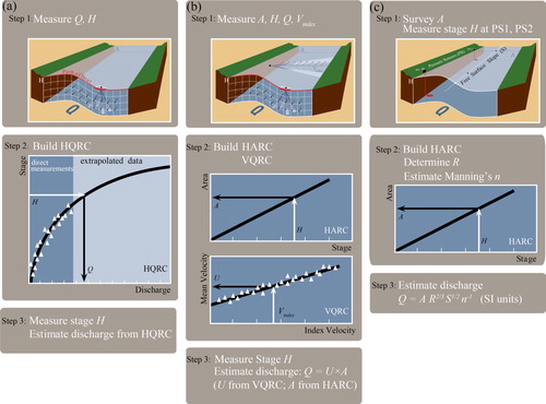
The HQRC, the first developed continuous monitoring method, is extensively described in Rantz (1982), Herschy (2009), and WMO (2010). The IVRC method has been pioneered with travel-time based acoustic instruments (Patino & Ockerman, 1997) and has become increasingly popular with the adoption of acoustic-Doppler velocity instruments for measurements in rivers. The conventional SA method was originally developed for extending the HQRC usability for high flows (Dalrymple & Benson, 1967). For this purpose, the free-surface slope determined from high-water marks produced by flood events along the stream path is used for discharge estimation (ISO:1070, 1992). With the advent of low-cost pressure transducers, the SA method has resurfaced as a new approach for continuous measurement of streamflow (Smith et al., 2010; Stewart et al., 2012). The simplified version of the CSA presented in this paper has been recently proof-tested through field experiments by the present authors (Lee et al., 2017; Muste et al., 2016; Muste et al., 2019).

Irrespective of the method, an essential criterion for their implementation is the selection of the measurement site in a manner that maximally ensures a quasi-uniform flow condition in the station vicinity (Rantz, 1982). The deployment of the instruments and construction of the ratings are guided by analytical and practical considerations that best accommodate local flow conditions (e.g. type of channel control for HQRC, coverage of a large portion of the cross-section and proper positioning of the velocity instrument for IVRC). Final ratings are established using an extended dataset of calibration and verification measurements that is processed with statistical tools. The overall accuracy of the discharge estimates via ratings reflects the operator skills in relation to the method by which the directly measured variables are combined to obtain the discharge estimates.

Currently, there is a continuous search for innovative solutions to overcome the operational limitations of the conventional approaches for continuous flow monitoring and for improving their accuracy. So far, the most promising results have been obtained with nonintrusive instruments for velocity measurements (based on optical, underwater acoustics, and radar principles) acquired with submersed, airborne, or remote-sensing deployments (Rennie et al., 2017). These new measurement techniques have different advantages and disadvantages, but none of them captures the flow velocity over the full cross-section, which would yield the desired direct discharge estimate.

The available hydrometric literature does not offer criteria for a comprehensive evaluation of the performance of the methods at hysteresis-prone sites nor for detecting the departure of the actual flows from the estimates provided by the conventional monitoring methods. There is no indication of systematic efforts for correcting or directly capturing hysteresis in the routine usage of conventional monitoring methods. While the monitoring methods have improved over time through the ingestion of new, superior instruments, the underlying protocols and associated assumptions have not been recently reviewed with respect to their capability for capturing hysteresis. Consequently, the ratings associated with HQRC and IVRC continue to be constructed assuming essentially one-to-one relationships between two flow variables without specifically distinguishing between flow phases. Given that a highly sophisticated method is typically required to outperform a much simpler rating curve approach, it is expected that new monitoring methods will be developed, screened, and evaluated in the near future.

3 Conceptualization of the hysteretic effect in monitoring methods

3.1 Analytical considerations

The first analytical considerations are presented for the simplest flow cases as the monitoring methods were initially developed for such cases. The methods for more complex flows were developed by building on protocols developed for simple flows. The simplest flow situation for a monitoring station is the uniform and steady flow in a rectangular prismatic channel, where the Manning equation applies (Henderson, 1966): (1) $Q_s\text{ = (1/}n\text{)}A{R}^{\text{2/3}}{S_o}^{\text{1/2}}=K{S_o}^{\text{1/2}}$(1) where Q_s is the flow discharge, n is Manning’s roughness coefficient, A is cross-sectional area, R is hydraulic radius, S_o is channel bed slope, and K = (1/n)AR^2/3 is the channel conveyance (in metric units). To attain uniform flow conditions, the channel cross-section should maintain its shape (i.e. A, R, and the flow depth, h, should be constant within the stream reach) along a straight streamwise direction. For such conditions, the streamwise gradients of the energy line (S_e), free-surface line (S_w), and streambed (S_o) are equal (Fig. 2a, left). Equation (1) used for guiding the construction of the HQRC ratings for in-bank flows leads to a one-to-one stage–discharge rating (Fig. 2a, centre). Using such ratings results in a simultaneous occurrence of the peaks for mean velocity, discharge, and depth (Fig. 2a, right).

Figure 2 Illustration of the hysteretic effect on the stage–discharge relationship: (a) streamwise gradients for energy and free-surface lines for steady uniform flows (left), stage–discharge ratings obtained with the one-to-one relationship (centre), and resultant hydrographs (right); (b) streamwise gradients for energy and free surface lines for unsteady flows (left), non-unique stage–discharge relationship (centre), and non-overlapping hydrographs (right). Notations are as provided in Eqs (1) and (2)

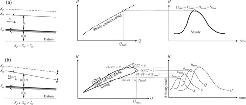
During unsteady flow propagating through a channel (i.e. flood wave), Eq. (1) is not strictly valid even if the channel maintains its cross-section and straight streamwise direction, as the free-surface slope is continuously changing during the flood wave progression. The occurrence of unsteady flow is inherently associated with flow non-uniformity, as illustrated in Fig. 2b (left). A more accurate description of such flows is provided by the one-dimensional Saint-Venant equations derived from principles of mass and momentum conservation applied to shallow-water flows (Chow, 1959). The Saint-Venant equations can take a variety of forms. For the present context, where we substantiate the departure of the unsteady flow from steady flow condition, the most useful relationship is the arrangement provided by Knight (2006) that relates the discharge in unsteady flow, Q, with the steady discharge, Q_s,as defined by Eq. (1): (2) $\begin{array}{rl}& Q=Q_s\sqrt{1-\frac{1}{S_o}\frac{\mathrm{\partial }h}{\mathrm{\partial }x}-\frac{U}{g{S}_o}\frac{\mathrm{\partial }U}{\mathrm{\partial }x}-\frac{1}{g{S}_o}\frac{\mathrm{\partial }U}{\mathrm{\partial }t}}\\ & \mathit{\text{kinematic wave}}\to |\\ & \mathit{\text{diffusion wave}}\to \to \to \to |\\ & \mathit{\text{fully dynamic wave}}\to \to \to \to \to \to \to \to \to \to \to |\end{array}$(2) where U is cross-section mean velocity, t is time, and x is distance along the channel. Equation (2) is valid under the following assumptions: incompressible fluid, one-dimensional flow, hydrostatic pressure distribution, and negligible vertical acceleration. For the present context, it should be mentioned that these conditions are essentially met if the best practice guidelines for site selection are applied (i.e. quasi-prismatic and straight channels without lateral inflows or outflows). Solving Eq. (2) with considerations of all its terms is a complex undertaking; therefore, recourse is made to numerical solutions or simplifying assumptions. Verification of this equation through experiments is possible but it would require measurements with the high frequency of all involved variables at one or two locations.

Equation (2) provides a realistic hydraulic description of the propagation of a flood wave irrespective of its type: kinematic (first term only), diffusion (first and second terms), or full dynamic (all terms). In other words, the type of wave resulting from rainfall within the station’s drainage area depends on the gauge-site location and event characteristics. During the wave propagation, the magnitude of the terms varies continuously, commensurate with the degree of dispersion and subsidence of the propagating waves (Ferrick, 1985; Henderson, 1966). More specifically, the type of waves for a specific site and event is determined by the relative importance of the terms in Eq. (2); i.e. when a term is an order of magnitude smaller than the others it can be discarded (Hunt, 1997). Consequently, the interplay among the magnitude of the terms in Eq. (2) leads to relationships between two flow variables that are distinct for the rising and falling limb of a wave propagating event, as illustrated in Fig. 2b (centre). It is to be noted that the flow depth, h, is derived from the stage, H, in hydrometric applications, and therefore their use in the present context is interchangeable. The non-unique (not single-valued) relationships Q = ƒ(H) for the unsteady flows are labelled “loops” (Henderson, 1966). A special case of Eq. (2) is the kinematic wave that displays minimal peak phasing, being equivalent from this perspective to the steady uniform flow situation (e.g. Lamberti & Pilati, 1990). This type of wave occurs typically on large slopes where the gravity force largely exceeds the inertia and pressure gradient forces; hence Eq. (2) reduces to Eq. (1). For all forms of non-kinematic waves, the flow variables follow distinct trajectories on the rising and falling limbs of the hydrographs.

There are many investigations discussing wave types and their characteristics (e.g. Dottori et al., 2009; Fread, 1985; Henderson, 1966; Moramarco et al., 2008; Perumal et al., 2004; Ponce & Simons, 1977; Yen & Tsai, 2001). Some of them provide practical guidelines for identification of the type of waves occurring at specific sites and particular events. For example, Julien (2002), Shen and Diplas (2010) and Ghosh (2014) recommend the use of the full dynamic wave for inland rivers (i.e., located outside coastal areas with tides) on mild and small bed slopes. For such settings, the propagation of large flow unsteadiness produces significant differences between discharge estimates obtained with HQRC ratings and the actual measurements (Di Baldassarre & Montanari, 2009; Dottori et al., 2009; Faye & Cherry, 1979; Fenton, 1999; Fenton & Keller, 2001; Fread, 1975). For large bed slopes, Aricò et al. (2009) recommend the use of only the first term in Eq. (2) which corresponds to the kinematic wave.

Another direct manifestation of the unsteady flows is the phase sequencing between the time series of the mean flow variables. The phase-sequencing, as well as the loops, are discussed in other research areas as being direct manifestations of the hysteresis effect (Prowse, 1984). Fig. 2b (right) illustrates that the peaks for the flow variables in unsteady flow are time-phased in the following order: energy, slope, velocity, discharge and flow stage. Previous studies demonstrate both analytically (e.g. Lee, 2013; Moots, 1938) and experimentally (e.g. Graf & Qu, 2004; Graf & Song, 1995; Hunt, 1997; Nezu et al., 1997; Nezu & Nakagawa, 1995; Qu, 2002) that the peak phasing is commensurate with the strength of the hysteresis, that in turn is directly dependent on the site conditions and dynamic characteristics of the wave. The phase sequencing of the hydrograph variable peaks has been rarely reported in hydraulic measurements acquired in field conditions (e.g. Rowinski et al., 2000). These authors used customized deployments with multiple instruments and measurement protocols to find differences of approximately 30 min between the free-surface slope and stage peaks for a small inland stream. For large rivers, this phasing can be considerably increased. Peaks of the order of 3.5 days are observed in an ongoing study (Sontek, personal communication, July 2018).

3.2 Impact of hysteretic behaviour on the monitoring methods

Ensuing from the above discussion on the balance between the magnitude of the terms in Eq. (2), it is important to reiterate that for the present context the main concerns are related to situations where non-kinematic waves occur. The non-kinematic flood waves lead to hysteresis behaviour, which is equivalent to asserting that hysteresis is a “property” of the non-kinematic waves. The subsequent discussions will focus only on this type of waves, as they are associated with the most significant impact on the accuracy of the conventional monitoring methods. As we will glean from Section 5.1, the non-kinematic waves are most likely to occur at gauging stations located in lowland areas exposed to intense storms. Often these locations and situations lead to flooding.

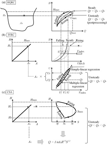
While the hysteretic behaviour produces distinct relationships between any two of the flow variables during the rising and falling stages of the unsteady flows, the hydrometric community most often associates the discussion on hysteresis with the HQRC relationship. This situation is understandable given that this rating has been and continues to be the most extensively used in streamflow monitoring. The steady HQRC method misses the hysteretic behaviour altogether, as can be seen from Fig. 3a. This is because the Q = ƒ(H) relationships for this method are the same for the rising and falling limbs of the hydrograph (dotted line in Fig. 3a). Correction as described below needs to be applied to the steady HQRC discharge estimates to recover the hysteretic loop associated with the passing of storms through the gauging station (continuous line in Fig. 3a). In contrast, the IVRC and CSA methods displayed in Fig. 3b and c can directly capture the hysteretic behaviour in the continuously measured variables during storm passing. Therefore, the discharge estimates obtained with these methods are also characterized by a hysteretic behaviour. The capability of IVRC and CSA methods to capture the hysteresis in the estimated discharges stems from the addition to the measured stage (a geometrical descriptor of the flow) of fast-sampled measurements of velocities across the section and free-surface gradients (kinematic descriptors of the flow), respectively. It is implicitly assumed herein that if hysteresis can be substantiated by a given measurement protocol (as illustrated in Fig. 2b (centre)), the associated time-phasing of the measured and estimated flow variables is captured as well.

Figure 3 Illustration of the hysteretic behaviour on continuous monitoring methods: (a) HQRC method, (b) IVRC method, and (c) CSA method. Notations are as provided in Fig. 1. Subscripts r, f, and s are for the rising limb of the hydrographs, the falling limb, and steady flows, respectively. Vⁱ denotes index velocity and H is the flow stage.

Adjusted HQRC method

There are abundant data and knowledge on the correction methods used for adjusting hysteresis on the one-to-one HQRC rating (Fig. 3a). Comprehensive reviews of correction methods are provided by Kennedy (1984), Schmidt (2002), and Dottori et al. (2009). The correction protocols are based on purely empirical or semi-empirical approaches (e.g. Jones, 1916; Rantz, 1982; Tawfik et al., 1997) or analytical models (e.g. Chow, 1959; Henderson, 1966; Ozbey, 2011; Petersen-Øverleir, 2006). Given that the correction application brings additional operational costs, the one-to-one HQRC ratings are typically used for both steady and unsteady flow situations. A relatively low-cost method was tested by the authors using a modified version of the Fread (1975) method (Lee & Muste, 2017). This method computes stage or discharge in unsteady flows by iteratively applying the full 1-D momentum equation and Manning’s equation in conjunction with the available steady based HQRC.

IVRC method

This method is recommended for measurements in areas where unsteady flow and/or backwater occur (Le Coz et al., 2008; Levesque & Oberg, 2012; Morlock et al., 2002). While the index-velocity method is increasingly used, the experimental evidence documenting its performance is still scarce and some more subtle aspects of the method continue to be investigated. For example, detailed laboratory studies (Graf & Qu, 2004; Nezu & Nakagawa, 1995; Song & Graf, 1996; Tu, 1992) and field measurements (Cheng et al., 2019; Muste & Lee, 2013; Nihei & Sakai, 2006) hint at the conclusion that the index to cross-sectional channel velocity rating is non-unique for the rising and falling stages of a storm wave, displaying the trends illustrated in Fig. 3b (bottom). This non-unique relationship can be produced by several factors (see also Section 5). The most important factor for the present context is that the magnitudes of the streamwise velocities on the rising limb are larger than those on the falling limb for the same flow depth (e.g. Hunt, 1997; Langhi et al., 2013; Song & Graf, 1996). The thickness of the resultant looped index-velocity rating is relatively smaller than the one in stage–discharge for the same site and event. Sometimes, these small differences in the IVRC rating may be obscured by the measurement uncertainty (especially if the hysteresis severity is not considerable).

CSA method

This method has been tested by a series of field experiments in a small stream located on a mild-sloped stream (Lee, 2013; Lee et al., 2017; Lee & Muste, 2017; Muste et al., 2019). The CSA implementation entails the following sequence (see also Fig. 1c): (a) deploy a pair (as a minimum) of stage sensors at the ends of an experimental reach and determine the free-surface slope from the direct stage measurements; (b) survey the perimeter of one of the cross-sections and determine the associated stage–area relationship; (c) determine the discharge using Eq. (1). The approach used in the CSA experiments is similar to the dynamic rating curve used by Dottori et al. (2009) where a dynamic slope is used in the Manning equation instead of a time-constant water-surface slope. The major difference between the two approaches is that the CSA method is applied to just one end of the channel reach. The premises for CSA implementation are that the selected channel geometry is quasi-uniform and straight with a practically constant discharge within the reach at any instant (i.e. ∂Q / ∂x ≈ 0). For the constant flow rate assumption to be realistic, the distance between the reach ends should be small and the free-surface slopes be acquired with fast sampling rates. The distance between the stage sensors cannot be, however, drastically reduced as the measured water-surface fall needs to be sufficiently large to not be hindered by the instrument resolution and water level fluctuations.

4 Hysteresis case studies

Presented below is a set of analytical, experimental, and numerical case studies aimed at substantiating features of the methods used at gauging stations for continuous discharge estimation in unsteady flow conditions. While we realize that a systematic illustration of hysteresis requires prior assessments of the sites and events to ensure the presence of unsteady flows that support sound illustrations of the phenomenon, the case studies presented below take advantage of relevant results from our previous research. These results are sufficient for illustrating salient features of the paper’s subject and provide quantitative estimates of the hysteresis magnitude for practical situations. For all the locations and situations, the propagating waves are of non-kinematic nature, as diagnosed with relations presented in Section 5.1. The results for the first and third cases were obtained from measurements conducted in a small natural stream, while the second case shows selected results from a field campaign in a medium-size stream reach located downstream from a hydropower station. The cases one and three illustrate that hysteresis is observable even in a small stream exposed to frequently occurring events (ISJP, 2016; Lee, 2013; Lee et al., 2017; Muste et al., 2019). The second case demonstrates the capabilities and limitations of the conventional HQRC and IVRC methods applied for unsteady flows developing at a site with a complex measurement environment, whereby the flow unsteadiness is significant and frequently occurring (Cheng et al., 2019).

4.1 Monitoring hysteresis with conventional methods

HQRC Adjusted with Fread method

The stream reach for this case study is located on a typical US Midwest stream, the Clear Creek (near Oxford, Iowa, USA). At this location, the streamflow is continuously monitored with a stage–discharge gauging station (USGS # 05454220) that closely follows the requirements for best practices recommended by the hydrometric guidelines. Flows through this station vary from 0.1 to 170 m³ s⁻¹; flows larger than 50 m³ s⁻¹ exceed the bankfull line leading to floodplain flooding. The correction method used for adjusting the HQRC rating is based on the Fread method (Fread, 1975) highlighted in Section 3.2.

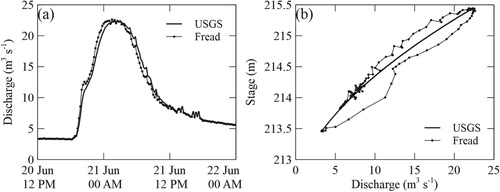
Figure 4a shows the discharges estimated with the USGS HQRC rating along with the adjusted stage–discharge relationship as provided by the “modified” Fread method (Lee & Muste, 2017). The modification has been deemed necessary as the original Fread method is applicable only for a long and slow-rising kinematic flood wave. The figure shows that the adjusted HQRC hydrograph precedes the USGS one for the analysed storm. Fig. 4b illustrates that the correction applied to the HQRC rating recovers the dynamics of the flood wave propagation that was missed by the USGS HQRC rating. Another notable observation is that the trace of the Fread correction is wrapped around the USGS stage–discharge rating. This appearance is not a general pattern for hysteresis loops, rather a customary feature of the Fread correction method whereby the HQRC curve serves as a basis in the computations. In the area of the maximum thickness of the loop, the stage difference for equal discharges and the discharge difference for equal stages are about ± 10%. This percentage difference is significantly larger than the typical ± 5% widely accepted in monitoring practice to account for the uncertainties associated with measurements of the flow variables and the construction of the stage–discharge rating.

Figure 4 Adjustment of the HQRC rating using the modified Fread method (Lee & Muste, 2017): (a) discharge time series for an unsteady event obtained with HQRC and Fread method; (b) comparison of the HQRC rating with the loop created by the applied correction

IVRC method

The stream reach for this case study is located on the Snake River immediately below the CJ Strike Dam in Idaho, USA (Cheng et al., 2019). This station, along with other gauging sites on this river, experiences frequent flow changes developing very fast (i.e. about 2 min) as they are triggered by opening or closing the gates leading to the turbines located in the dams. Motivated by concerns related to the accuracy of discharge estimates provided by the HQRC-based method during unsteady flows, the station’s hydrologists adopted the IVRC method as an alternative monitoring approach. Multiple-linear regression in determining the mean velocities, that accounts for stage variation in addition to index velocity, rather than the simple regression, is used for this station as recommended by best practice in IVRC guidelines.

This case study entails a comparison of discharges acquired directly or estimated continuously during a controlled experiment with: (a) Winter–Kennedy meters (WKM) set in the turbine housings; (b) IVRC-based rating; (c) HQRC-based ratings; and (d) transect (i.e. cross-section) measurements with acoustic Doppler current profilers (ADCP). The time series for discharges estimated with the four alternative methods are illustrated in Fig. 5a. For steady flow situations, the simultaneous measurements acquired with these methods show differences within ± 5% compared to WKMs considered as reference for the present analysis. During flow transitions, the direct ADCP transect measurements are relatively close to the WKM meters, while the HQRC and IVRC estimates display noticeable differences. An alternative view of the differences during the transitions is shown in Fig. 5b, where the simultaneous measurements with the four methods in the familiar stage–discharge relationship are displayed. The maximum difference between discharges for the same flow stage during the upward and downward transitions is 80% for HQRC vs. WKM and 40% for IVRC vs. WKM. For completeness of the comparison, the HQRC estimates corrected with the “modified” Fread formula discussed above are also added in Fig. 5b.

Figure 5 Customized experiment for the assessment of the capabilities of various monitoring methods in unsteady flows: (a) discharge time series during the experiment; (b) discharge estimates provided by WKM, IVRC, HQRC and HQRC corrected with the Fread (1975) method; (c) the variation of the index velocity during flow transitions; (d) index-velocity vs mean channel velocity relationship during flow transitions

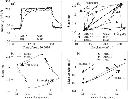
Figure 5c displays the variation of the index-velocity data plotted against the flow stage during the flow transition periods. It can be noted from this figure that the index velocities are considerably different for upward and downward flow changes and exhibit sharp velocity peaks at the beginning of the transitions. These differences are also reflected in the relationship between the index- and mean-velocity obtained with multiple linear regression ratings (Fig. 5d). Previous laboratory experiments (Nezu et al., 1997; Tu, 1992), field measurements (Holmes, 2016), and simulations (Lee, 2013) indicate that the loop thickness is proportional to the index-velocity change rate. It should be noted that the IVRC method can also develop loops from factors other than flow unsteadiness, i.e. improper synchronization for the variable time series (Ruhl & Simpson, 2005). We verified our data to address this concern and found that this cause was not involved in the reported results.

4.2 Monitoring hysteresis with CSA method

Experimental arrangement and methodology

The performance of the CSA method for unsteady flows is demonstrated with a set of data collected at the Clear Creek site (the same site as for the first case but for a different deployment period). For this experiment, the pair of pressure transducers were set 156-m apart and continuously sampled every 3 min (Muste et al., 2019). The inputs for Eq. (1), the basis for CSA method, include the geometry of the cross-section obtained from local surveys, assumed Manning’s roughness coefficient, and the continuous measurements of the free-surface slope over the experimental channel reach. Manning’s n-stage rating specific for the site was developed to account for its variation with stage and the vegetation growth on the channel banks. An associated assumption in using this equation is that flow displays comparable velocity heads at the ends of the experimental channel and they can be discarded (Fenton & Keller, 2001, p. 54). In effect, the drop in water-surface profile compensates for the energy losses caused by the friction of the flow at the channel bed and banks and the changes in the free-surface produced by the flow unsteadiness.

Experimental results

The discharges recorded by the USGS HQRC station during the deployment of the CSA experiments during the spring of 2017 are provided in Fig. 6a. The subsequent discussion is focused on the 17 June 2017 event that was sufficiently intense to produce hysteresis. Time series of the analysed flow variables are smoothed using a moving average over five consecutive data points with averages reported every 3 min (Fig. 6b). The comparison of the USGS and the CSA-derived discharge estimates for the event shows an overall good agreement, as shown in Fig. 6b. The USGS estimates were adjusted for the flood wave travel time between the two neighbouring stations, i.e. about 250 m. A low bias of 16% for the CSA method compared to the USGS rating estimates is observable for the low-value flows. A high bias of 8% is noted for the peak flow.

Figure 6 Discharge time series for: (a) the monitoring interval; (b) Storm 4 on 17 June 2017

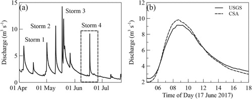
A potential explanation for the bias at low flows is that discharges under 3.75 m³ s⁻¹ are controlled by local bed features rather than channel control. As for the bias at the hydrograph peak, similar trends have been reported in previous studies with the SA method (Jarrett, 1987). Furthermore, Di Baldassarre and Montanari (2009) found that during unsteady flows, the conventional HQRC rating can underestimate up to 15% of the actual discharge values. Along the same line, Fenton (2001) explains analytically that the high bias at the peak flow demonstrates that the maximum flow of diffusive flood waves is larger (and occurs earlier) than the flow computed from simple stage–discharge rating. An additional factor explaining the near-peak flow bias might be related to the fact that the reliability of the USGS rating for the higher flow range is not as robust as for lower flow range, because the density of the calibration/verification measurements are less dense for high flows. There are insufficient data in the USGS records to confidently test this assertion.

Figure 7a shows the variation of the water-surface slope with stage measured at the downstream cross-section. The plot illustrates distinct slope paths for the event’s rising and falling stages. Fig. 7b illustrates the stage–discharge relationship obtained with the CSA method. In the area of maximum loop thickness, the differences between the discharges for the same stage and the stages for the same discharge are 16% and 15%, respectively. The USGS HQRC data are not considered in this figure as the channel cross-sections for the USGS and CSA stations are at different locations. Another reason for not directly comparing the ratings is that the CSA method uses the actual roughness (i.e. corresponding to the vegetation stage as of June 2017) for discharge estimation, while the USGS rating is not adjusted for seasonal vegetation growth. More specifically, the actual Manning’s n values were adjusted to account for changes in the flow stage as well as for changes due to riparian vegetation growth, as illustrated in Fig. 7c. The adjustment entailed a compound formula (i.e. different n-values for the bed and banks) for estimation of the roughness coefficient and comparison of photographic evidence of the site with available lookup tables for the same vegetation type and season (Coon, 1998). The impact of Manning’s coefficient variation accounting for depth variation and vegetation growth is shown in Fig. 7d where the stage–discharge rating using the actual n is plotted against a constant n value over the perimeter, i.e. assuming the bed roughness as the representative for the whole cross-section as is often done in practice.

Figure 7 Hysteretic effects on flow variable dependencies captured with the CSA method during the 17 June 2017 event: (a) free-surface slope; (b) stage–discharge relationship; (c) the change in Manning’s roughness with stage and the vegetation growth on the channel banks; (d) effect of stage variation and vegetation-induced roughness on the measurements with CSA; (e) peak phasing of the flow variables; (f) hysteretic loops created by the propagation of the main seasonal storms illustrated in Fig. 6a

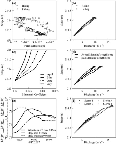
Figure 7e illustrates the phase sequencing of the peaks of the mean flow variables discussed in Section 3.2. The CSA experiments substantiate the following peak sequence: the free-surface slope first, the channel bulk velocity (determined by dividing the discharge across the cross-sectional area) second, and the stage third. The raw data for the plots displayed in Fig. 7e are averaged over a number of data points to better illustrate the trends in the peak phasing. Finally, Fig. 7f illustrates the loops produced by all prominent storms captured by the CSA method during the spring of 2017. The CSA peak discharges for all these storms are larger than those estimated by the USGS rating (see also Fig. 6a), with larger hysteresis thickness for the greater and more intense storms.

4.3 Numerical simulations

The inclusion of the numerical simulations in the present discussion is motivated by the desire to compare and complement the data acquired through field experiments. Moreover, today’s increased access to simulation models leads more often to the use of numerical surrogates along with streamflow gauging estimates for the investigation of various stream-transport problems (ISJP, 2016). For the present context, we tested a 1-D model widely used for simulating progressing fluvial floods (Altinakar et al., 2009); i.e. the HEC-RAS software fit with the unsteady module incorporating the full set of Saint-Venant equations (Gray, 2008). The model was set up for the experimental site described in Section 4.2 and the Storm 4 event of the spring of 2017. To test the sensitivity of the HEC-RAS model to boundary conditions, two simulations were carried out. Both simulations use discharges provided by the USGS gauge 05454220 (practically collocated with the CSA station) as an upstream boundary condition. For the first simulation, the normal depth at the downstream boundary with energy slope equal to the average bed slope of the modelled stream reach was used. For the second simulation, the observed stage by the sensor located at the end of the experimental reach was used as a downstream boundary condition. For both modelling cases, Manning’s roughness coefficient accounting for stage and vegetation growth variation (i.e. labelled the “actual n” in Fig. 7c) was used. The setting and execution of the HEC-RAS simulations followed typical protocols as specified by the Gray (2008) guidelines (e.g. selection of the time step and number of iterations).

Both the HEC-RAS simulations and the CSA results display non-unique stage–discharge relationships. However, the loops are much less evident in the results of the numerical simulations compared with those provided by the CSA method. For both simulation alternatives, the output discharge is, as expected, constant along the river reach and peaks at the same value (i.e. 9.15 m³ s⁻¹). This value is slightly smaller than the discharge estimated with the CSA method (i.e. 10.54 m³ s⁻¹). Notably, both simulation scenarios indicate the expected sequence of the peak variable arrival, i.e. energy line gradient and velocity first, followed by a free-surface slope, as shown in Fig. 2b (right). However, the time difference between the energy gradient line and discharge differs drastically between the two modelling scenarios: 14 min for the normal depth scenario and 4.75 h for the one using the measured stages. The difference between the free-surface slope and stage peaks is 1.5 h for the CSA method, as shown in Fig. 7e. The aforementioned observations on the simulation results lead to the inference that the HEC-RAS using normal depth dampens the dynamics of the flow (hysteresis thickness and the peak phasing patterns) compared to both HEC-RAS using the observed CSA stages as downstream boundary condition as well as in comparison with the CSA free-surface slope measurements.

While not closely aligned with the present discussion focused on monitoring methods, a short review of the causes of the discrepancies between the experimental and numerical results offers useful hints on the capabilities and limitations of the simulations tools. It is known that the accuracy of the HEC-RAS results depends on: model setting (e.g. length of the modelled stream reach, cross-section spacing), the quality of boundary conditions used for simulation, assumptions used in modelling, and the parameters used for model execution (Gray, 2008). One immediate shortcoming of our HEC-RAS simulations might be the length of the modelled reach that is too short to develop a uniform flow. For such a situation, an energy slope needs to be provided that is subsequently used by the HEC-RAS model to automatically back-calculate depth using Manning’s equation. A good choice for the value of energy slope is hard to make without computations, so errors associated with the assumed energy slope are expected. Another shortcoming might be related to the grid resolution and the Courant number (used for checking the simulation convergence). Errors are expected if the computational grid is overly coarse in comparison with the modelled flood wavelengths (typically unknown for practical situations). Our HEC-RAS simulations might be affected by both sources of errors.

Further explanations of the differences between measured and simulated results require consideration of more subtle details related to how the HEC-RAS simulations handle various types of flood waves. While the propagation of the kinematic wave is independent of the downstream boundary condition, for the diffusive wave (as it is in our case) a physically meaningful boundary condition is required (Ferrick et al., 1984). This is well captured in our simulations with boundary conditions defined by actual observations or assumed values for the normal depth. Yen and Tang (1977) and Pappenberger et al. (2006) comment that the use of assumed rather than observed boundary conditions can produce simulation errors that can largely exceed other sources of modelling uncertainty.

5 Discussion

The hysteretic behaviour associated with unsteady channel flows is rooted in differences between the rising and falling stages of the unsteady flows. The changes are not limited to the mean flow characteristics but they also entail changes in the distribution of turbulence (Bareš et al., 2008; Hunt, 1997; Nezu & Nakagawa, 1995; Yang & Chow, 2008). Consequently, the relationships between mean flow variables for the rising limb of a hydrograph are distinct from those on the falling limb and the timing of the flow variable peaks is not in phase. While hysteresis is a process known to monitoring agencies, it has only received attention in major flood-prone areas along large rivers (e.g. Mississippi) with the purpose to provide more accurate data for streamflow forecasting models (Holmes, 2016). Hysteresis occurring in medium and small inland rivers is, in most cases, undocumented as there is a perception in the hydrometry community that the impact of hysteresis is small and cannot be discerned from instrument uncertainty (Holmes, 2016). Currently, there are neither systematic efforts for assessing the presence of hysteresis at gauging stations nor studies to evaluate its impact on streamflow estimation in medium and small rivers.

Our case studies entail medium and small streams located on intermediate and low-slope terrains exposed to fast-varying flows, situations prone to developing non-kinematic waves. These lower inland streams are often located in areas of intensively-managed landscapes (due to agricultural activities and urbanization) that lead to higher flow peaks and accelerated waves that further exacerbate the development of hysteresis (Schober et al., 2015). To make the situation worse, the climatic changes lead to more frequent and intense events and eventually to more devastating floods (e.g. Mallakpour & Villarini, 2015; Messner & Meyer, 2006). For such situations, the availability of accurate monitoring methods operating continuously and unsupervised would greatly benefit flood mitigation efforts.

The most substantial inference from the present paper is that the hysteresis produces a non-unique relationship between any two of the flow variables associated with the currently used streamflow monitoring methods. This non-unique relationship can be recreated for the HQRC method through post-processing corrections and can be directly captured by IVRC and CSA methods. The subsequent discussion shows that there are means to detect both the likelihood of hysteresis occurrence at a specific site as well as improved means to assess the severity of hysteresis impact on various types of ratings.

5.1 Sensitivity of hysteresis to site and event characteristics

The loops schematically illustrated in Figs 2 and 3 are visual depictions of the hysteresis effect. It is well known that steep-sloped streams produce kinematic waves where the hysteresis loop is negligible. Mild-sloped streams tend to produce considerable hysteretic-loop sizes if the hydrograph duration is short and its magnitude is large. Ponce (1989) demonstrated that the loops developed by dynamic waves are larger than those produced by diffusion waves. Given the variety of responses to the wave types, there have been attempts to define parameters and associated thresholds to indicate when and where hysteresis is significant and what the expected magnitude of the hysteretic loop is (Lee & Muste, 2017). These hysteresis “diagnostic” formulas have been obtained either analytically (Mishra & Seth, 1996; Moussa & Bocquillon, 1996; Ponce, 1989) or from laboratory and field experiments (Dottori et al., 2009; Graf & Suszka, 1985; Moramarco et al., 2008; Nezu et al., 1997; Song & Graf, 1996; Takahashi, 1969). Selected hysteresis diagnostic formulas are provided in Table 1. The use of the diagnostic formulas allows us to distinguish the type of flood wave produced for a given site and event (i.e. kinematic, diffusion or dynamic). For example, implementation of the diagnostic formula suggested by Mishra and Seth (1996) to the data collected with the CSA method presented in Section 4.2 results in η parameter values of 0.035, 0.039, 0.08 and 0.06 for Storms 1, 2, 3 and 4 (Fig. 6a). These values indicate that all the storms propagating through this gauging station are of diffusive nature.

Table 1 Hysteresis diagnostic approaches (Lee, 2013)

Reference	Criterion description
Takahashi (1969)	λ = Vs /(c × sin θ) where Vs = (hp − hb)/Td; Td = duration from the base discharge to the peak discharge; sin θ = bed slope, So; the parameter λ implies the ratio of the rising speed of water surface (Vs) to the vertical component of celerity c of long waves; c = (g × hp)^1/2
Fread (1975, 1985)	Insignificant when So > 0.001 for 0 < dh/dt < 1.219 m h^−1; moderately significant when 0.0001 < So < 0.001 for 0.030 < dh/dt < 0.914 m h^−1; significant when So < 0.0001 for dh/dt > 0.015 m h^−1
Graf and Suszka (1985)	Γ = (1/u*b) × (Δh/ΔT) where u*b is the friction velocity the base flow, Δh is the difference of the maximum and base flow depth; ΔT = the duration of the hydrograph
Ponce (1989)	τ = TSoV/D where T = wave period, commonly taken to be twice the time of the rise of the flood wave; V = reference flow mean velocity; D = reference flow depth. For τ > 171, the kinematic wave approximation was found to be reasonable (i.e. hysteresis occurs when τ < 171 – diffusive wave)
Nezu and Nakagawa (1995)	A = (1/Uc) × Vs where Uc = convection velocity of turbulent eddies ≈ (Ub + Up)/2. The authors indicated that Takahashi’s method (1969) is not suitable for unsteady flows over smooth beds, and therefore a new relationship is proposed by replacing c × sin θ with Uc.
Mishra and Seth (1996)	Wave type	Hysteresis, η	Wave number $\hat{\sigma }$ and $\hat{\sigma }{\mathsf{F}}_{\text{o}}$	Phase difference, $\phi$
	Kinematic	η < 0.025	$\hat{\sigma }$ ≤ 0.030	$\phi$ < 0.030
	Diffusion	0.025 ≤ η ≤ 0.10	$\hat{\sigma }{\mathsf{F}}_{\text{o}}$ ≤ 0.462	0.030 ≤ $\phi$ ≤ 0.130
	Dynamic	η > 0.10	$\hat{\sigma }{\text{F}}_{\text{o}}$ > 0.462	$\phi$ > 0.130
Dottori et al. (2009)	So ≥ 5 × 10^−4 (steep slope). A good estimation of kinematic or quasi-kinematic conditions

The ability to identify the type of wave developing for specific sites and flow situations is critical for guiding the type of rating acceptable for the gauging and for selecting the appropriate numerical model for each situation. The guidance can be obtained for both new and existing monitoring sites with careful analysis of the site’s hydro-morphological characteristics, i.e. the topography of the site and associated flow dynamics. The best information on flow dynamics can be obtained with direct measurements of the discharge, adopting an event-based tracking approach. In the absence of direct measurements, analysis of the discharge records accumulated over long-term intervals or their estimates along with topographic data can be used as surrogates for input in the hysteresis diagnostic formulas. If streamflow data are not available (i.e. at new gauging sites), surrogate estimates derived from regional regression analysis can be used as input in the hysteresis diagnostic formulas.

The hysteresis produced by multiple events at a site appears as multiple loops bundled in a “cloud”, as illustrated for the stage–discharge relationship in Fig. 7f. This cloud is interpreted as a conceptual uncertainty interval produced by hysteresis around the one-to-one HQRC relationship (Schmidt, 2002) as it is caused by simplifying assumptions associated with the applied analysis. These uncertainties can be considerable. For example, Faye and Cherry (1979), Di Baldassarre and Montanari (2009) and Herschy (2009) report discharge differences for the same stage ranging from 9.8% to 34% in large rivers. Differences up to 40% were found between direct ADCP discharge measurements and stage–discharge estimates in a medium-size, low bed-slope river (Muste & Lee, 2013). Typically, these uncertainties are not assessed and reported for the evaluation of the monitoring method performance.

5.2 Time phasing of hydrographs

While closely related to the hysteretic behaviour discussed above, the hydrograph phasing due to unsteady flow has received much less attention in previous studies. The handful of studies on the flow variable hydrograph phasing occurring during the propagating of non-kinematic waves converges on the hydrograph sequencing illustrated in Fig. 2b (right). This sequence was demonstrated analytically through studies conducted by Moots (1938) and Lamberti and Pilati (1990). The mean velocity-discharge-stage (U-Q-h) peak sequence is also confirmed by laboratory experiments (e.g. Graf & Qu, 2004) as well as with field measurements with the IVRC method (e.g. Cheng et al., 2019) and the CSA method (e.g. Muste et al., 2019). The peak phasing is considerably larger in field conditions compared with laboratory experiments due to the scaling effect involved in hydraulic modelling. The peak phasing for the intrinsically-connected energy gradient line (S), friction velocity (u_*), and water free-surface gradient (S_w) has been much less observed. When observed, the peaks for the above gradient hydrographs were found to precede the U-Q-h peak sequence as shown in laboratory experiments (e.g. Tu, 1992), field studies (e.g. Rowinski & Czernuszenko, 1998), and numerical simulations (e.g. Ghimire & Deng, 2011). Our CSA experiments and the associated numerical simulations described in Sections 4.2 and 4.3 confirm that the free-surface slope peaks before the U-Q-h peak sequence (see also Fig. 7e).

If a given discharge monitoring method can capture hysteresis in the flow variables, it is implicit that it can distinguish the peak sequencing. This is of immediate importance for characterizing flooding whereby the “flagging” of the peak of a variable that precedes the stage can then be used in conjunction with analytical or statistical approaches to forecast the timing of the floodwave peak arrival (Todini, 2004). Such capabilities have important implications beyond hydrometric applications. For example, there are multiple experimental field studies that report peaks of suspended sediment concentrations preceding those of discharges during storm hydrographs (e.g. Gellis, 2013; Tabarestani & Zarrati, 2015; Yang & Lee, 2018). While in these publications the peak phasing is not related to hysteresis, the reported results reinforce the inherent features of the hysteretic behaviour of the flow variables, as discussed above. From this perspective, it is apparent that calculations of the sediment loads for suspended sediment (or any other matter in suspension) transported during unsteady flow using methods that do not capture hysteresis in the stage–discharge relationships (such as estimated in, for example, Gao & Josefson, 2012; Humphries et al., 2012; Wilson et al., 2012) are inaccurate.

5.3 Outlook

There is an obvious lack of synergy between the available knowledge on river mechanics and the underlying principles used to monitor unsteady flows. Specifically, the construction of the ratings used by conventional monitoring methods is based on quasi-random observations of the events, combined with statistical analysis. It is suggested herein that the adoption of an event-based monitoring approach and use of a suitable analytical formulation for the specific flow situation (i.e. steady or unsteady state) is a better alternative in constructing the ratings. It should be mentioned that in addition to the procedural shortcoming used to build the ratings, the analytical basis for building the monitoring method protocols for monitoring unsteady flow poses also concerns. Most of them are related to Manning’s formula for expressing resistance in Eqs (1) and (2) and Manning’s n coefficient that is associated with the channel boundary roughness (Yen, 2002). Manning’s formula does not apply to streams with dune beds or shallow flows over gravel (e.g. Ferguson, 2010). Moreover, recent studies show that the use of Manning’s formula in Eq. (2) is not adequate for unsteady flows (e.g. Bombar, 2016; Ghimire & Deng, 2011; Rowinski et al., 2000). The actual impact of violating this assumption for practical purposes is still under investigation (e.g. Mrokowska et al., 2015). On the other hand, use of empirically-determined Manning’s n coefficients from field measurements in new situations can be subjective and clumsy (e.g. Barnes, 1967; Kean & Smith, 2005), and can even result in common flow situations, in errors as high as ± 29% (Bray, 1979). In addition, roughness varies with the flow stage and has a time dimension when vegetation-induced roughness is involved (Arcement & Schneider, 1989; Coon, 1998). To further complicate the matter, it is mentioned that the bed and vegetation conditions might change during the same storm event if the intensity of the unsteady flow is significant (Gunawan, 2010). While the above-mentioned complexities are not discussed in detail, they are mentioned here as any of them can affect the interpretation of the hysteretic behaviour on the monitoring methods.

Unfortunately, there are few coherent efforts to accelerate the translation of the available knowledge on unsteady flows to the practice of stream monitoring. Therefore, further enhancement of the performance of the monitoring methods should be focused first on revisiting their fundamentals and comprehensively assessing their accuracy (e.g. Di Baldassarre & Montanari, 2009). Some preliminary considerations for improvements in monitoring methods are suggested below.

HQRC

The use of the conventional one-to-one stage–discharge relationship can be considered adequate for all rivers at steady and uniform conditions, as well as for flood waves exhibiting kinematic behaviour. For all the other cases, the gradients of the energy line are strongly influenced by the changes in inertia and pressure forces that ultimately lead to the formation of loops in the stage–discharge relationship. If one of the diagnostic formulas described in Section 5.1 signals the presence of hysteresis at the gauging site, the use of the correction methods for HQRC discussed in Section 4.1 is necessary, irrespective of the stream size. This suggestion is perhaps the most important highlight of this study as the vast majority of the world’s gauging stations are based on conventional stage–discharge ratings.

This corrected data can be subsequently investigated for hysteresis impact with analytical methods used in conjunction with data-mining applied to existing long-term discharge records. Among the latest methods are approaches based on neural networks (e.g. Bhattacharya & Solomatine, 2005; Boogaard et al., 1998; Deka & Chandramouli, 2003; Sudheer & Jain, 2003; Tawfik et al., 1997; Wolfs & Willems, 2014), advanced numerical solvers (e.g. Fenton, 2019; Liu & Hodges, 2014), modelling in conjunction with the data collected for the stage–discharge relationship (e.g. Wijbenga et al., 2013), or fuzzy logic modelling (e.g. Lohani et al., 2006; Takagi & Sugeno, 1985). The use of the aforementioned methods is especially recommended for flood-prone areas subjected to extreme events as the flood inundation maps created under the assumption of steady-state flows underestimates the extent of inundated areas (Dawdy, 2007).

IVRC

While IVRC-based stations equipped with acoustic instruments are gaining popularity, they continue to be scrutinized for several method-specific concerns. Among them, of primary importance is the optimum positioning of the probes in the cross-section. The position of the probe is sensitive to the changes in the velocity profile shape, hence affecting the outcomes of IVRC during unsteady flows. An additional concern is related to the fact that it is common for acoustic instruments to profile only a small portion of the cross-section. One solution to this issue is the use of hybrid methods for developing the IVRC ratings. These methods combine assumed velocity profiles in the vertical or spanwise directions with directly acquired velocities (Hidayat et al., 2011; Kästner et al., 2018; Nihei & Kimizu, 2008; Nihei & Sakai, 2006). An increasingly popular hybrid approach is based on the principle of maximum entropy (Chiu & Chen, 2003) as adopted by Morse et al. (2010) and Chen et al. (2012). Finally, it is recommended to continue investigating the performance of the IVRC method when used in steady and unsteady flows (Jackson et al., 2012; Le Coz et al., 2008; Muste & Lee, 2013) as well as assessing the accuracy using rigorous uncertainty analyses (e.g. González-Castro & Chen, 2005; Over et al., 2017).

In parallel with pursuing studies that address the above concerns, it is recommended to test the feasibility of adopting the “segmented” approach for constructing the IVRC rating. This approach entails accounting for different phases of the flow during the passing of flood wave propagation similar to the protocols used for coastal rivers subjected to tides (Ruhl & Simpson, 2005). This empirical approach entails the construction of separate ratings for the flood-to-web flow and the ebb-to-flood phases without considering the stage as an additional independent variable in the IVRC construction. The extension of this protocol would be assumed to separately construct the IVRC rating for rising and falling limbs of the hydrographs. This approach seems to be suitable for the construction of both HQRC and IVRC methods applied to inland rivers, irrespective of their degree of unsteadiness, as typically the steady flows are covering the lower parts of the flow variable hydrographs.

CSA

The results presented in this paper show that the use of Eq. (1), in conjunction with fast sampled water-surface slopes, provides a good hydraulic approximation for describing unsteady flows propagating as non-kinematic waves. This conclusion is in agreement with the analytical studies of Ferrick et al. (1984), who revealed that the water-surface slope in Eq. (1) is largely responsible for the creation of a diffusive-type wave that in turn is the primary factor in developing hysteresis. The presented results highlight an important practical advantage of the CSA method compared with both HQRC and IVRC alternatives through its capability to adequately capture both hysteresis in the flow variables as well as phased sequencing of the peaks, whereby water-surface hydrograph peaks first.

The need to further investigate the performance of the CSA method is also recommended, as the use of its underlying equations continues to expand in conjunction with new measurement approaches. For example, a Manning-based approach is currently tested with satellite-based instruments capable to quantify free-surface gradients in large rivers (Bjerklie et al., 2005; Brakenridge et al., 2012). The acquired data is subsequently fed in Manning-like equations along with inferences obtained from regression analyses applied to ground-based stream width and free-surface slope measurements (Schaperow et al., 2019).

The above considerations highlight that the improvement of the current monitoring methods can be attained by reviewing their fundamentals, assessing the capabilities of the new measurement technologies thoroughly, and adopting smart, data-driven algorithms that can provide reliable real-time data irrespective of the site and flow situation. Subsequently, related practical issues should be considered. Among them are: estimation of the streamflow magnitude and its timing (e.g. Pappenberger et al., 2006), the assessment of the flow volumes passed by streams during unsteady flows (e.g. Ferrer et al., 2013; Ozbey, 2011), and evaluation of transport processes driven by unsteady flows (e.g. Graf & Suszka, 1985; Humphries et al., 2012; Morehead et al., 2003).

6 Conclusions

The analytical and experimental evidence presented in this paper illustrates some of the strengths and limitations of the most commonly used methods for continuous discharge monitoring of unsteady river flows. The main focus of the present discussion is on flood waves propagating as non-kinematic waves. First, it is reiterated that the simple HQRC relationship completely misses hysteresis produced by unsteady flows. The peak of the propagating wave is larger and occurs earlier than the one indicated by the conventional HQRC peak. The hydrographs of the flow variables during unsteady flows do not occur simultaneously; rather they peak in the following order: energy-line gradients, velocity, discharge, and stage. The HQRC ratings are typically corrected for hysteresis effects in post-processing, hampering the use of data in real-time. Second, there are clear indications that the IVRC and CSA methods can detect most of the hysteretic behaviour, but the accuracy of their estimation for different situations needs to be further investigated. Third, the paper demonstrates that currently there are means to build on the existing analytical methods, legacy data, and advancement in sensing and computer technologies to improve our capabilities to enhance the accuracy of flow measurements during unsteady flows.

The present analysis and the conclusions drawn herein are, however, based on limited datasets. From this perspective, the outcomes of the discussion should be regarded as being indicative rather than confirmative. However, we hope that the present discussion reveals that the effect of hysteresis on monitoring methods deserves additional and substantial research. There is an obvious need for systematic scrutiny of the hysteretic behaviour by posing some overarching questions first:

• Where and when does hysteresis occur and how significant it is?

• What are the practical implications of hysteresis presence for monitoring method users?

• What are the best means to account for and use hysteresis for enhancing the streamflow monitoring capabilities?

The sound evaluation of the principles of the available monitoring methods in combination with the adjustment of new technologies for their enhancement has the potential to predict the initiation and the expected shapes of the hysteresis loops irrespective of the river size and unsteady flow situation. The new technologies are not limited to acoustic instruments and also include emerging techniques based on image- or radar-based principles. The combination of new technologies with suitable analytical modules applied to data measured in real-time will secure stream gauge networks enabling enhanced exploration in river science and robust support for the many practical aspects of river monitoring.

Notation

A	=	cross-sectional area (m2)
AA	=	cross-sectional area for an arbitrary stage lower than bankfull (m2)
c	=	celerity of waves (m)
D	=	reference flow depth (m)
F0	=	Froude number
g	=	gravity acceleration (m s−2)
h	=	flow depth (m)
hb	=	flow depth at the base discharge (m)
hmax	=	maximum flow depth (m)
hp	=	flow depth at the peak discharge (m)
H	=	stage (m)
HA	=	an arbitrary stage lower than bankfull (m)
K	=	channel conveyance (m3 s−1)
n	=	Manning’s roughness coefficient (–)
Q	=	stream discharge, generic term for either steady or unsteady flow (m3 s−1)
Qf	=	unsteady flow discharge for the falling limb of the hydrograph (m3 s−1)
Qmax	=	maximum discharge (m3 s−1)
Qr	=	unsteady flow discharge for the rising limb of the hydrograph (m3 s−1)
Qs	=	steady flow discharge (m3 s−1)
R	=	hydraulic radius (m)
S	=	gradient of the energy line, generic term for either steady flow or unsteady flow (–)
Se	=	gradient of the energy line (–)
Smax	=	maximum gradient of the energy line (–)
So	=	gradient of the streambed (–)
Sw	=	gradient of the free-surface line (–)
t	=	time (s)
T	=	wave period (s)
Td	=	duration from the base discharge to the peak discharge (s)
u*b	=	friction velocity of the base flow (m s−1)
U	=	cross-sectional mean velocity (m s−1)
Uc	=	convection velocity of turbulent eddies (m s−1)
Ub	=	convection velocity of turbulent eddies at the base flow (m s−1)
Up	=	convection velocity of turbulent eddies at the peak flow (m s−1)
Uf	=	cross-sectional mean velocity for the falling limb of the hydrograph (m s−1)
Umax	=	maximum cross-sectional mean velocity (m s−1)
Ur	=	cross-sectional mean velocity for the rising limb of the hydrograph (m s−1)
V	=	reference flow mean velocity (m s−1)
Vi	=	index velocity measured by the sensor at specified elevation (m s−1)
$V_f^i$	=	index velocity measured by the sensor at specified elevation for the falling limb (m s−1)
$V_r^i$	=	index velocity measured by the sensor at specified elevation for the rising limb (m s−1)
${V_s}^i$	=	index velocity measured by the sensor at specified elevation for steady flows (m s−1)
Vindex	=	index velocity, generic term (m s−1)
Vs	=	rising speed of water surface (m s−1)
x	=	distance along the channel (m)
z(x)	=	elevation of the channel bed (m)
α	=	non-dimensional hysteresis parameter (–)
Γ	=	non-dimensional hysteresis parameter (–)
Δh	=	difference of the maximum and base flow depth (m)
ΔT	=	duration of the hydrograph (s)
η	=	non-dimensional hysteresis parameter (–)
θ	=	angle (°)
λ	=	non-dimensional hysteresis parameter (–)
$\hat{\sigma }$	=	wave number (–)
τ	=	non-dimensional hysteresis parameter (–)
$\phi$	=	phase difference (rad)

Acknowledgements

This paper greatly benefited from the review and discussions with M. Altinakar (University of Mississippi, USA), N. Ozbey (Akarsu, Ankara, Turkey), I. Fujita (Kobe University, Japan), and R. Tsubaki (Nagoya University, Japan). The substantial input from V. Nikora (University of Aberdeen, UK) and M. Ghidaoui (The Honk Kong University of Science and Technology, Hong Kong) has greatly improved the original manuscript. Heartfelt thanks to the many students who contributed for almost a decade to the acquisition of the in situ data presented in this paper.

Additional information

Funding

The first author acknowledges the partial support provided by National Science Foundation (NSF) Division of Earth Sciences (EAR) Award # 1331906. This work is also supported by the Korea Agency for Infrastructure Technology Advancement (KAIA) grant funded by the Ministry of Land, Infrastructure and Transport (Grant 20AWMP-B121100-05). M. Rojas Oliveros and F. Quintero were supported for this work by the Iowa Flood Center, a research group at IIHR-Hydroscience & Engineering, The University of Iowa that is funded by the Iowa State legislature.

References

- Altinakar, M. S., Matheu, E. E., & McGrath, M. Z. (2009, September 27–October 1). New generation modeling and decision support tools for studying impacts of dam failures. [Paper presentation]. Proc., Association of State Dam Safety Officials Dam Safety 2009 Annual Conf.
- Arcement, G., Jr., & Schneider, V. (1989). Guide for selecting manning’s roughness coefficients for natural channels and flood plains United States geological survey water-supply paper 2339. Water-Supply Paper, 2339, 6–8. https://doi.org/10.3133/wsp2339
- Aricò, C., Nasello, C., & Tucciarelli, T. (2009). Using unsteady-state water level data to estimate channel roughness and discharge hydrograph. Advances in Water Resources, 32(8), 1223–1240. https://doi.org/10.1016/j.advwatres.2009.05.001
- Bareš, V., Jirák, J., & Pollert, J. (2008). Spatial and temporal variation of turbulence characteristics in combined sewer flow. Flow Measurement and Instrumentation, 19(3-4), 145–154. https://doi.org/10.1016/j.flowmeasinst.2007.06.002
- Barnes, H. H. (1967). Roughness characteristics of natural channels. US Government Printing Office.
- Bhattacharya, B., & Solomatine, D. P. (2005). Neural networks and M5 model trees in modelling water level–discharge relationship. Neurocomputing, 63, 381–396. https://doi.org/10.1016/j.neucom.2004.04.016
- Bjerklie, D. M., Moller, D., Smith, L. C., & Dingman, S. L. (2005). Estimating discharge in rivers using remotely sensed hydraulic information. Journal of Hydrology, 309(1-4), 191–209. https://doi.org/10.1016/j.jhydrol.2004.11.022
- Bombar, G. (2016). Hysteresis and shear velocity in unsteady flows. Journal of Applied Fluid Mechanics, 9(2), 839–853. www.jafmonline.net
- Boogaard, H., Gautam, D. K., & Mynett, A. E. (1998, August 24–26). Auto-regressive neural networks for the modelling of time series. Proceedings of Hydroinformatics Conference, Copenhagen, Denmark.
- Brakenridge, G. R., Cohen, S., Kettner, A. J., De Groeve, T., Nghiem, S. V., Syvitski, J. P., & Fekete, B. M. (2012). Calibration of satellite measurements of river discharge using a global hydrology model. Journal of Hydrology, 475, 123–136. https://doi.org/10.1016/j.jhydrol.2012.09.035
- Bray, D. I. (1979). Estimating average velocity in gravel-bed rivers. Journal of the Hydraulics Division, 105(9), 1103–1122.
- Chen, Y.-C., Yang, T.-M., Hsu, N.-S., & Kuo, T.-M. (2012). Real-time discharge measurement in tidal streams by an index velocity. Environmental Monitoring and Assessment, 184(10), 6423–6436. https://doi.org/10.1007/s10661-011-2430-y
- Cheng, Z., Lee, K., Kim, D., Muste, M., Vidmar, P., & Hulme, J. (2019). Experimental evidence on the performance of rating curves for continuous discharge estimation in complex flow situations. Journal of Hydrology, 568, 959–971. https://doi.org/10.1016/j.jhydrol.2018.11.021
- Chiu, C.-L., & Chen, Y.-C. (2003). An efficient method of discharge estimation based on probability concept. Journal of Hydraulic Research, 41(6), 589–596. https://doi.org/10.1080/00221680309506891
- Chow, V. T. (1959). Open channel flow. London: McGraw-Hill, 11(95), 99, 136–140.
- Coon, W. F. (1998). Estimation of roughness coefficients for natural stream channels with vegetated banks (Vol. 2441, p. 145). US Geological Survey.
- Dalrymple, T., & Benson, M. A. (1967). Measurement of peak discharge by the slope-area method: U.S. geological survey techniques of water-resources investigations, book 3, chap. A2, p. 12.
- Dawdy, D. R. (2007). Prediction versus understanding (the 2006 Ven Te Chow lecture). Journal of Hydrologic Engineering, 12(1), 1–3. https://doi.org/10.1061/(ASCE)1084-0699(2007)12:1(1)
- Deka, P., & Chandramouli, V. (2003). A fuzzy neural network model for deriving the river stage—discharge relationship. Hydrological Sciences Journal, 48(2), 197–209. https://doi.org/10.1623/hysj.48.2.197.44697
- Di Baldassarre, G., & Montanari, A. (2009). Uncertainty in river discharge observations: A quantitative analysis. Hydrology & Earth System Sciences, 13(6), 913–921. https://doi.org/10.5194/hess-13-913-2009
- Dottori, F., Martina, M., & Todini, E. (2009). A dynamic rating curve approach to indirect discharge measurement. Hydrology and Earth System Sciences, 13(6), 847–863. https://doi.org/10.5194/hess-13-847-2009
- Faye, R. E., & Cherry, R. N. (1979). Channel and dynamic flow characteristics of the Chattahoochee river, Buford Dam to Georgia highway 141: River-quality assessment of the upper Chattahoochee river basin, Georgia (Vol. 2063). Department of the Interior, Geological Survey.
- Fenton, J. D. (1999, August 22–27). Calculating hydrographs from stage records. [Paper presentation]. Proc. 28th IAHR Congress, Graz.
- Fenton, J. D. (2001, November 28–30). Rating curves: Part 1-correction for surface slope [Paper presentation]. 6th Conference on Hydraulics in Civil Engineering: The State of Hydraulics, Proceedings, Hobart, Tasmania.
- Fenton, J. D. (2019). Flood routing methods. Journal of Hydrology, 570, 251–264. https://doi.org/10.1016/j.jhydrol.2019.01.006
- Fenton, J. D., & Keller, R. J. (2001). The calculation of streamflow from measurements of stage. CRC for Catchment Hydrology.
- Ferguson, R. (2010). Time to abandon the Manning equation? Earth Surface Processes and Landforms, 35(15), 1873–1876. https://doi.org/10.1002/esp.2091
- Ferrer, C., Moreno, M., & Sanchez, R. (2013, May 15–16). The influence of hysteresis in the development of stage-discharge relationships. [Paper presentation]. Congress SHF Hydrometrie.
- Ferrick, M. G. (1985). Analysis of river wave types. Water Resources Research, 21(2), 209–220. https://doi.org/10.1029/WR021i002p00209
- Ferrick, M. G., Bilmes, J., & Long, S. E. (1984). Modeling rapidly varied flow in tailwaters. Water Resources Research, 20(2), 271–289. https://doi.org/10.1029/WR020i002p00271
- Fread, D. (1975). Computation of stage-discharge relationships affected by unsteady flow. Journal of the American Water Resources Association, 11(2), 213–228. https://doi.org/10.1111/j.1752-1688.1975.tb00674.x
- Fread, D. (1985). Channel routing. Hydrological forecasting/edited by MG Anderson and TP Burt.
- Gao, P., & Josefson, M. (2012). Event-based suspended sediment dynamics in a central New York watershed. Geomorphology, 139-140, 425–437. https://doi.org/10.1016/j.geomorph.2011.11.007
- Gellis, A. C. (2013). Factors influencing storm-generated suspended-sediment concentrations and loads in four basins of contrasting land use, humid-tropical Puerto Rico. Catena, 104, 39–57. https://doi.org/10.1016/j.catena.2012.10.018
- Ghimire, B., & Deng, Z.-Q. (2011). Event flow hydrograph-based method for shear velocity estimation. Journal of Hydraulic Research, 49(2), 272–275. https://doi.org/10.1080/00221686.2011.552463
- Ghosh, S. N. (2014). Flood control and drainage engineering. Oxford & IBH Publishing.
- González-Castro, J. A., & Chen, Z. (2005, May 15–19). Uncertainty of index-velocity measurements at culverts. World Water and Environmental Resources Congress 2005, Anchorage, Alaska, United States. https://doi.org/10.1061/40792(173)450
- Graf, W., & Qu, Z. (2004). Flood hydrographs in open channels. Proceedings of the Institution of Civil Engineers-Water Management, 157(1), 45–52. https://doi.org/10.1680/wama.2004.157.1.45
- Graf, W., & Song, T.-C. (1995). Bed-shear stress in non-uniform and unsteady open-channel flows. Journal of Hydraulic Research, 33(5), 699–704. https://doi.org/10.1080/00221689509498565
- Graf, W., & Suszka, L. (1985). Unsteady flow and its effect on sediment transport [Paper presentation]. 21st IAHR Congress, 13–18 August 1985, Melbourne, Australia.
- Gray, W. B. (2008). HEC-RAS rivers analysis system user manual. US Army Corps of Engineers, Hydrologic Engineering Center Crop.
- Gunawan, B. (2010). A study of flow structures in a two-stage channel using field data, a physical model and numerical modelling [Doctoral dissertation, University of Birmingham]. https://etheses.bham.ac.uk/id/eprint/669/
- Henderson, F. M. (1966). Open channel flow. Macmillan.
- Herschy, R. (2009). Streamflow measurement (3rd ed.). Taylor & Francis.
- Hidayat, H., Vermeulen, B., Sassi, M., Torfs, P., & Hoitink, A. (2011). Discharge estimation in a backwater affected meandering river. Hydrology and Earth System Sciences, 15(8), 2717–2728. https://doi.org/10.5194/hess-15-2717-2011
- Holmes, R. (2016, July 11–14). River rating complexity, Proceedings of the International Conference on Fluvial Hydralics (River Flow 2016), St. Louis, USA.
- Humphries, R., Venditti, J. G., Sklar, L. S., & Wooster, J. K. (2012). Experimental evidence for the effect of hydrographs on sediment pulse dynamics in gravel-bedded rivers. Water Resources Research, 48(1). https://doi.org/10.1029/2011WR010419
- Hunt, A. E. (1997). The behaviour of turbulence in unsteady open channel flow [Ph.D. thesis, University of Canterbury]. https://ir.canterbury.ac.nz/handle/10092/7722
- ISJP. (2016). Iowa bridge sensor demonstration project, Iowa silver jackets program report. The University of Iowa.
- ISO:1070. (1992). Liquid flow measurement in open channels – Slope-area method. International Organization for Standardization.
- Jackson, P. R., Johnson, K. K., & Duncker, J. J. (2012). Comparison of index velocity measurements made with a horizontal acoustic Doppler current profiler (2328-0328). US Department of the Interior, US Geological Survey.
- Jarrett, R. D. (1987). Errors in slope-area computations of peak discharges in mountain streams. Journal of Hydrology, 96(1-4), 53–67. https://doi.org/10.1016/0022-1694(87)90143-0
- Jones, B. E. (1916). A method of correcting river discharge for a changing stage (Vol. Water Supply Paper 375, pp. 117–130). US Government Printing Office.
- Julien, P. (2002). River mechanics. River mechanics.
- Kästner, K., Hoitink, A., Torfs, P., Vermeulen, B., Ningsih, N. S., & Pramulya, M. (2018). Prerequisites for accurate monitoring of river discharge based on fixed-location velocity measurements. Water Resources Research, 54(2), 1058–1076. https://doi.org/10.1002/2017WR020990
- Kean, J. W., & Smith, J. D. (2005). Generation and verification of theoretical rating curves in the Whitewater river basin, Kansas. Journal of Geophysical Research: Earth Surface, 110(F4). https://doi.org/10.1029/2004JF000250
- Kennedy, E. (1984). Discharge ratings at gaging stations: US Geological survey techniques of water-resources investigations, book 3, chap. A10, 59.
- Knight, D. (2006). River flood hydraulics: validation issues in one-dimensional flood routing models. Taylor & Francis.
- Lamberti, P., & Pilati, S. (1990). Quasi-kinematic flood wave propagation. Meccanica, 25(2), 107–114. https://doi.org/10.1007/BF01566211
- Langhi, M., Hosoda, T., & Dey, S. (2013). Velocity deformation model for unsteady open-channel flows over smooth and rough beds. Journal of Hydraulic Engineering, 139(4), 433–443. https://doi.org/10.1061/(ASCE)HY.1943-7900.0000677
- Le Coz, J., Pierrefeu, G., & Paquier, A. (2008). Evaluation of river discharges monitored by a fixed side-looking Doppler profiler. Water Resources Research, 44(4). https://doi.org/10.1029/2008WR006967
- Lee, K. (2013). Evaluation of methodologies for continuous discharge monitoring in unsteady open-channel flows [Doctoral dissertation, The University of Iowa]. https://ir.uiowa.edu/etd/5012/
- Lee, K., Firoozfar, A. R., & Muste, M. (2017). Technical note: Monitoring of unsteady open channel flows using the continuous slope-area method. Hydrology & Earth System Sciences, 21, 1863–1874. https://doi.org/10.5194/hess-21-1863-2017
- Lee, K., & Muste, M. (2017). Refinement of the Fread method for improved tracking of stream discharges during unsteady flows. Journal of Hydraulic Engineering, 143(6), Article 06017003. https://doi.org/10.1061/(ASCE)HY.1943-7900.0001280
- Levesque, V. A., & Oberg, K. A. (2012). Computing discharge using the index velocity method. US Department of the Interior, US Geological Survey.
- Liu, F., & Hodges, B. R. (2014). Applying microprocessor analysis methods to river network modelling. Environmental Modelling & Software, 52, 234–252. https://doi.org/10.1016/j.envsoft.2013.09.013
- Lohani, A., Goel, N., & Bhatia, K. (2006). Takagi–Sugeno fuzzy inference system for modeling stage–discharge relationship. Journal of Hydrology, 331(1-2), 146–160. https://doi.org/10.1016/j.jhydrol.2006.05.007
- Mallakpour, I., & Villarini, G. (2015). The changing nature of flooding across the central United States. Nature Climate Change, 5(3), 250–254. https://doi.org/10.1038/nclimate2516
- Messner, F., & Meyer, V. (2006). Flood damage, vulnerability and risk perception–challenges for flood damage research. In Jochen Schanze, Evzen Zeman, & Jiri Marsalek (Eds), Flood risk management: Hazards, vulnerability and mitigation measures (pp. 149–167). Springer.
- Mishra, S., & Seth, S. (1996). Use of hysteresis for defining the nature of flood wave propagation in natural channels. Hydrological Sciences Journal, 41(2), 153–170. https://doi.org/10.1080/02626669609491489
- Moots, E. (1938). A study in flood waves—University of Iowa Studies in Engineering. Bull, 14. https://ir.uiowa.edu/cgi/viewcontent.cgi?article=1014&context=uisie
- Moramarco, T., Pandolfo, C., & Singh, V. P. (2008). Accuracy of kinematic wave approximation for flood routing. II. Unsteady analysis. Journal of Hydrologic Engineering, 13(11), 1089–1096. https://doi.org/10.1061/(ASCE)1084-0699(2008)13:11(1089)
- Morehead, M. D., Syvitski, J. P., Hutton, E. W., & Peckham, S. D. (2003). Modeling the temporal variability in the flux of sediment from ungauged river basins. Global and Planetary change, 39(1-2), 95–110. https://doi.org/10.1016/S0921-8181(03)00019-5
- Morlock, S. E., Nguyen, H. T., & Ross, J. H. (2002). Feasibility of acoustic Doppler velocity meters for the production of discharge records from US geological survey streamflow-gaging stations (Vol. 1). US Department of the Interior, US Geological Survey.
- Morse, B., Richard, M., Hamaï, K., Godin, D., Choquette, Y., & Pelletier, G. (2010). Gauging rivers during all seasons using the Q2D velocity index method. Journal of Hydraulic Engineering, 136(4), 195–203. https://doi.org/10.1061/(ASCE)HY.1943-7900.0000143
- Moussa, R., & Bocquillon, C. (1996). Criteria for the choice of flood-routing methods in natural channels. Journal of Hydrology, 186(1-4), 1–30. https://doi.org/10.1016/S0022-1694(96)03045-4
- Mrokowska, M., Rowinski, P., & Kalinowska, M. (2015). A methodological approach of estimating resistance to flow under unsteady flow conditions. Hydrology & Earth System Sciences, 19(10), 4041–4053. https://doi.org/10.5194/hess-19-4041-2015
- Muste, M., Bacotiu, C., & Thomas, D. (2019, September 1–6). Evaluation of the slope-area method for continuous streamflow monitoring. [Paper presentation]. Proceedings of the 38th World Congress, Panama City.
- Muste, M., Cheng, Z., Firoozfar, A. R., Tsai, H.-W., Loeser, T., & Xu, H. (2016, July 11–14 ). Impacts of unsteady flows on monitoring stream flows. [Paper presentation]. River Flow Conference, St Louis, MO.
- Muste, M., & Hoitink, T. (2017). Measuring flood discharge. Oxford Research Encyclopedia of Natural Hazard Science.
- Muste, M., & Lee, K. (2013, September 8–13). Quantification of hysteretic behavior in streamflow rating curves. [Paper presentation]. Proceedings of the 35th IAHR World Congress, Chengdu.
- Nezu, I., Kadota, A., & Nakagawa, H. (1997). Turbulent structure in unsteady depth-varying open-channel flows. Journal of Hydraulic Engineering, 123(9), 752–763. https://doi.org/10.1061/(ASCE)0733-9429(1997)123:9(752)
- Nezu, I., & Nakagawa, H. (1995). Turbulence measurements in unsteady free-surface flows. Flow Measurement and Instrumentation, 6(1), 49–59. https://doi.org/10.1016/0955-5986(95)93458-7
- Nihei, Y., & Kimizu, A. (2008). A new monitoring system for river discharge with horizontal acoustic Doppler current profiler measurements and river flow simulation. Water Resources Research, 44(4). https://doi.org/10.1029/2008WR006970
- Nihei, Y., & Sakai, T. (2006, September 6–8 ). Study on river-discharge measurements with a bottom-mounted ADCP. [Paper presentation]. Proceedings of International Conference on Fluvial Hydraulics, Lisbon.
- Over, T. M., Muste, M., Duncker, J. J., Tsai, H.-W., Jackson, P. R., Johnson, K. K., Engel, F. E., & Prater, C. M. (2017, July 9–12). Uncertainty analysis of an index velocity meter and discharge computations at the Chicago sanitary and ship canal near Lemont, Illinois [Paper presentation]. Proceedings of the Hydraulic Measurement and Experimental Methods Conference, University of New Hampshire, Durham, NH.
- Ozbey, N. (2011, 26 June–1 July ). Adjustment factors for unsteady State-discharge measurements [Paper presentation]. Proceedings of the 34th World Congress of the International Association for Hydro-Environment Research and Engineering: 33rd Hydrology and Water Resources Symposium and 10th Conference on Hydraulics in Water Engineering, Brisbane, Australia.
- Pappenberger, F., Matgen, P., Beven, K. J., Henry, J.-B., & Pfister, L. (2006). Influence of uncertain boundary conditions and model structure on flood inundation predictions. Advances in Water Resources, 29(10), 1430–1449. https://doi.org/10.1016/j.advwatres.2005.11.012
- Patino, E., & Ockerman, D. (1997). Computation of mean velocity in open channels using acoustic velocity meters. US Department of the Interior, US Geological Survey.
- Perumal, M., Shrestha, K. B., & Chaube, U. (2004). Reproduction of hysteresis in rating curves. Journal of Hydraulic Engineering, 130(9), 870–878. https://doi.org/10.1061/(ASCE)0733-9429(2004)130:9(870)
- Petersen-Øverleir, A. (2006). Modelling stage—discharge relationships affected by hysteresis using the Jones formula and nonlinear regression. Hydrological Sciences Journal, 51(3), 365–388. https://doi.org/10.1623/hysj.51.3.365
- Ponce, V. M. (1989). Engineering hydrology: Principles and practices (Vol. 640). Prentice Hall.
- Ponce, V. M., & Simons, D. B. (1977). Shallow wave propagation in open channel flow. Journal of the Hydraulics Division, 103(12), 1461–1476. https://cedb.asce.org/CEDBsearch/record.jsp?dockey=0007750, http://ponce.sdsu.edu/shallowwave1461view.html
- Prowse, C. W. (1984). Some thoughts on lag and hysteresis. Area, 16(1), 17–23.
- Qu, Z. (2002). Unsteady open-channel flow over a mobile bed. Ecole Polytechnique Federale de Lausanne.
- Rantz, S. E. (1982). Measurement and computation of streamflow (Vol. 2175). US Department of the Interior, Geological Survey.
- Rennie, C., Hoitink, A. J. F., & Muste, M. (2017). Experimental hydraulics: Methods, instrumentation, data processing and management, volume II: Instrumentation and measurement techniques, chapter 6. CRC Press.
- Rowinski, P. M., & Czernuszenko, W. (1998, August 31–September 3). Friction and turbulent velocities in a river under unsteady conditions. [Paper presentation]. Third International Conference on Hydro-Science and Engineering.
- Rowinski, P. M., Czernuszenko, W., & Marc, J.-M. (2000). Time-dependent shear velocities in channel routing. Hydrological Sciences Journal, 45(6), 881–895. https://doi.org/10.1080/02626660009492390
- Ruhl, C. A., & Simpson, M. R. (2005). Computation of discharge using the index-velocity method in tidally affected areas. US Department of the Interior, US Geological Survey.
- Schaperow, J. R., Li, D., Margulis, S. A., & Lettenmaier, D. P. (2019). A curve-fitting method for estimating bathymetry from water surface height and width. Water Resources Research, 55(5), 4288–4303. https://doi.org/10.1029/2019WR024938
- Schmidt, A. R. (2002). Analysis of stage-discharge relations for open-channel flows and their associated uncertainties. University of Illinois at Urbana-Champaign.
- Schober, B., Hauer, C., & Habersack, H. (2015). A novel assessment of the role of Danube floodplains in flood hazard reduction (FEM method). Natural Hazards, 75(1), 33–50. https://doi.org/10.1007/s11069-013-0880-y
- Shen, Y., & Diplas, P. (2010). Modeling unsteady flow characteristics of hydropeaking operations and their implications on fish habitat. Journal of Hydraulic Engineering, 136(12), 1053–1066. https://doi.org/10.1061/(ASCE)HY.1943-7900.0000112
- Smith, C. F., Cordova, J. T., & Wiele, S. M. (2010). The continuous slope-area method for computing event hydrographs (2328-0328). U.S. Geological Survey.
- Song, T.-C., & Graf, W. (1996). Velocity and turbulence distribution in unsteady open-channel flows. Journal of Hydraulic Engineering, 122(3), 141–154. https://doi.org/10.1061/(ASCE)0733-9429(1996)122:3(141)
- Stewart, A. M., Callegary, J. B., Smith, C. F., Gupta, H. V., Leenhouts, J. M., & Fritzinger, R. A. (2012). Use of the continuous slope-area method to estimate runoff in a network of ephemeral channels, southeast Arizona, USA. Journal of Hydrology, 472-473, 148–158. https://doi.org/10.1016/j.jhydrol.2012.09.022
- Sudheer, K., & Jain, S. (2003). Radial basis function neural network for modeling rating curves. Journal of Hydrologic Engineering, 8(3), 161–164. https://doi.org/10.1061/(ASCE)1084-0699(2003)8:3(161)
- Tabarestani, M. K., & Zarrati, A. (2015). Sediment transport during flood event: A review. International Journal of Environmental Science and Technology, 12(2), 775–788. https://doi.org/10.1007/s13762-014-0689-6
- Takagi, T., & Sugeno, M. (1985). Fuzzy identification of systems and its applications to modeling and control. IEEE Transactions on Systems, Man, and Cybernetics, SMC-15(1), 116–132. https://doi.org/10.1109/TSMC.1985.6313399
- Takahashi, H. (1969). Theory of one-dimensional unsteady flows in a prismatic open channel. Ann. Dis. Prev. Res. Inst., Kyoto University, 12, 515–527.
- Tawfik, M., Ibrahim, A., & Fahmy, H. (1997). Hysteresis sensitive neural network for modeling rating curves. Journal of Computing in Civil Engineering, 11(3), 206–211. https://doi.org/10.1061/(ASCE)0887-3801(1997)11:3(206)
- Todini, E. (2004). Role and treatment of uncertainty in real-time flood forecasting. Hydrological Processes, 18(14), 2743–2746. https://doi.org/10.1002/hyp.5687
- Tu, H. (1992). Velocity distribution in unsteady open-channel flow over gravel beds. J. of Hydroscience and Hydraulic Eng., JSCE, 10, 11–25.
- Wijbenga, A., Paarlberg, A., & Schwanenberg, D. (2013). Optimizing flood forecasts with data-assimilation and a dynamic stage discharge relation, comprehensive flood risk management – Klijn & Schweckendiek (eds) (pp. 1479–1485). Taylor & Francis Group.
- Wilson, C., Papanicolaou, A., & Denn, K. (2012). Quantifying and partitioning fine sediment loads in an intensively agricultural headwater system. Journal of Soils and Sediments, 12(6), 966–981. https://doi.org/10.1007/s11368-012-0504-2
- WMO. (2010). Manual on stream gauging, volume 1–fieldwork. World Meteorological Organization.
- Wolfs, V., & Willems, P. (2014). Development of discharge-stage curves affected by hysteresis using time varying models, model trees and neural networks. Environmental Modelling & Software, 55, 107–119. https://doi.org/10.1016/j.envsoft.2014.01.021
- Yang, C. C., & Lee, K. T. (2018). Analysis of flow-sediment rating curve hysteresis based on flow and sediment travel time estimations. International Journal of Sediment Research, 33(2), 171–182. https://doi.org/10.1016/j.ijsrc.2017.10.003
- Yang, S. Q., & Chow, A. T. (2008). Turbulence structures in non-uniform flows. Advances in Water Resources, 31(10), 1344–1351. https://doi.org/10.1016/j.advwatres.2008.06.006
- Yen, B. C. (2002). Open channel flow resistance. Journal of Hydraulic Engineering, 128(1), 20–39. https://doi.org/10.1061/(ASCE)0733-9429(2002)128:1(20)
- Yen, B. C., & Tang, W. H. (1977, August 2–4). Reliability of flood warning. [Paper presentation]. Stochastic Processes in Water Resources Engineering, Proceedings 2nd International Conference on Stochastic Hydraulics, Lund, Sweden.
- Yen, B. C., & Tsai, C.-S. (2001). On noninertia wave versus diffusion wave in flood routing. Journal of Hydrology, 244(1-2), 97–104. https://doi.org/10.1016/S0022-1694(00)00422-4