Free-surface behaviour of shallow turbulent flows

Abstract

Over the last two decades, interest in the free-surface behaviour of gravity-driven shallow turbulent flows has increased considerably. It is believed that observation of free-surface behaviour can provide useful information about the hydrodynamic characteristics of the flow and enable remote retrieval of these characteristics to non-invasively and rapidly monitor river flows. At the current state the literature presents scattered knowledge and also exhibits non-uniformity in the terminology used. This paper is a review of the state-of-art of this area of research and was created with two objectives: to gather the information relevant to understand the linkages between the free-surface behaviour and underpinning hydrodynamic processes while using a uniform terminology, and to analyse the gaps in our knowledge of this critical topic.

Keywords:

• Air–water interface interactions
• free surface
• gravity-capillary waves
• open channel flows
• surface behaviour
• surface–hydrodynamics interactions
• turbulence-induced waves

View correction statement:

Correction

1 Introduction

There are many factors that govern the dynamics of streams, rivers and other open channel flows. From a macroscopic point of view, the major parameters that define these flows are the flow rate, the roughness of the boundaries, the shape of the flow section, the position of the free surface, the channel slope and the presence of major flow disturbing elements such as bridge piers, boulders and in-channel vegetation. Among the more minor factors are bedforms, bed grain size distribution, bed porosity and permeability, the entrainment risk of the bed material, local changes in the channel slope and bed morphology. The free-surface interface represents the dynamic upper boundary of an open channel flow system, therefore it seems reasonable to suggest that the free surface is also influenced by the same parameters. As a result, the extent of such parameter influence may be observed in the dynamically rough shape of the moving free surface, leading to the hypothesis that hydrodynamic flow characteristics might be inferred from the observation and interpretation of the free-surface behaviour.

Since the nineteenth century, the air–water interface and its relations with the underlying hydrodynamics have been the subject of several studies (Lamb, 1932; Rayleigh, 1883; Thomson, 1886). Recent improvements in numerical techniques, better performance of computers and enhanced capability to collect accurate digital, space- and time-resolved data (Marcus & Fonstad, 2010) have allowed a better understanding of the flow dynamics as well as the development of new applications such as remote monitoring. A number of researchers have suggested that the study of rivers’ free surface can enable non-invasive monitoring of their flow characteristics (Cooper et al., 2006; Dolcetti, 2017; Fujita et al., 2007; Krynkin et al., 2014; Legleiter et al., 2017; Nichols, 2013; Savelsberg et al., 2006). The free-surface behaviour also regulates the transfers of gas (Turney & Banerjee, 2013), heat (Lakehal et al., 2003), and scalars (Nagaosa & Handler, 2012) between the water flow and the atmosphere, and it can be a useful indicator to monitor riverine habitats, as in Milan et al. (2010). There are currently many techniques to remotely estimate specific flow properties. These are mostly based on optical principles (Muste et al., 2008; Nichols & Rubinato, 2016), but others use acoustics (Fukami et al., 2008; Horoshenkov & Nichols, 2012; Nichols et al., 2013) or radio waves (Plant et al., 2005). Only a few of these techniques have had a practical application in the field. Non-contact measurement technologies are improving continuously, but despite the rapid spread of applications, the actual understanding of the physical principles behind the free-surface behaviour and its measurements are still limited (Marcus & Fonstad, 2010).

The above reasons made us to realize that it is of interest now to critically assess the existing knowledge of the free-surface behaviour of gravity-driven shallow turbulent flows and to present the key advances in the form of a review. The target of this work is to assist the development of new measurement and analysis techniques. The existing literature is approached from an application-based perspective, focusing on studies that provide directly usable information to link free-surface observations with flow conditions. For this reason, more theoretical works about the physical details of the process beyond what is easily measurable in realistic field conditions, or numerical studies focused on simulation approaches rather than on observable results, are not discussed in detail. For more information on these topics, we refer to the works of Borue et al. (1995), Gabreil et al. (2018), Guo and Shen (2010), Shen et al. (1999) and Tsai (1998). In order to further focus the paper, only spatially and temporally homogeneous single-phase flow conditions are explored. Highly energetic flows and transitional flows (e.g. hydraulic jumps) that exhibit specific complexities (such as aeration) are beyond the scope of this work. An interested reader is encouraged to explore other studies that focus on such flow conditions, e.g. Chanson (2009), Longo (2010), Longo (2011), Toombes and Chanson (2007) or Valero and Bung (2018). This review also excludes film flows, as these have been the subject of a recent review by Aksel and Schörner (2018).

The paper is organized in the following manner: Section 2 reviews a seminal work of Brocchini and Peregrine (2001) as this provides a suitable framework within which to explore other studies; Section 3 describes the main mechanisms that govern free-surface dynamics; Section 4 presents a review of the most influential studies of free-surface shallow turbulent flows which have attempted to establish relationships between the bulk flow parameters and the free-surface pattern; key findings are then discussed in Section 5; and in Section 6 conclusions are derived and gaps in the knowledge are summarized along with recommendations as to how these may be addressed.

2 The dynamics of strong turbulence at free surfaces

The air–water interface is the complex and dynamically changing upper boundary of a free-surface flow. Despite the scientific and practical interest in determining the extent and manner in which hydrodynamic processes can influence the behaviour of the free surface, the topic has only attracted interest in recent years. A significant publication is by Brocchini and Peregrine (2001). Although this work was not specifically focused on shallow flows, it provided a useful conceptual framework to analyse the behaviour of free-surface flows when influenced by the underlying turbulence structures with various length scales and energy quantities. The framework therefore covers a broad range of conditions that occur in nature.

Brocchini and Peregrine (2001) realized that there was a lack of knowledge about the behaviour of the free surface in “strong” turbulent flows, where “strong” turbulence was defined as “sufficiently energetic that it causes the free surface to be strongly distorted” (Brocchini & Peregrine, 2001, p. 225). Examples of distortions can be the generation of surface waves, water ejections, dimples (point-like depressions of the surface) and surface breakup. The authors suggested that the balance between turbulent velocities and length scales is the reason for the various forms of deformation of the free surface, and proposed a two-parameter framework in which the stabilizing forces of gravity and surface tension are compared to the free-surface effects produced by the turbulence (Fig. 1). The strength of these stabilizing energy densities could have been described by the dimensionless Froude and Weber numbers (parameters that express the influence of the flow inertia with respect to the gravitational force and surface tension, respectively). However, the authors preferred to use dimensional variables in order to directly convey the magnitude of the observed surface quantities for the different hydrodynamic regimes. These two-dimensional parameters were defined through the characteristics of “blobs” described as “moderately coherent and discrete volumes of fluid that move upward to the surface, perhaps through it, sometimes falling back on it, or moving parallel to it and hence disturbing it” (Brocchini & Peregrine, 2001, pp. 233–234). These “blobs” have a typical length scale L and velocity q that are representative of the turbulent motion and were considered mutually independent. The definition of the size of the parameter L was imprecise and in practical situations this was assumed to be associated to the length of the most energetic turbulent scale or the length scale of dominant surface features. For the sake of simplicity, the norm of the velocity vector was preferred for q.

Figure 1 L-q diagram for water flows. Dotted lines represent Eq. (1), while the dashed line represents the limit corresponding to R_e,BP = 100. Shaded areas represent regions of marginal breaking and are zones where dotted lines could potentially lie (Brocchini & Peregrine, The dynamics of strong turbulence at free surfaces. Part 1. Description. Journal of Fluid Mechanics, 449, 225–254, 2001, reproduced with permission)

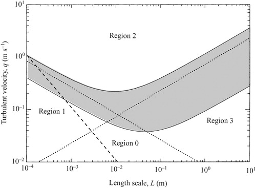
Brocchini and Peregrine (2001) organized their length–velocity L-q diagram (Fig. 1) into four regions according to unique Froude and Weber numbers that they defined as F_BP = q/(2gL)^1/2 and W_e,BP = ρ_f q²L/(2 T), respectively. Here g is the gravitational acceleration, ρ_f is the fluid density and T is the surface tension of the air–water interface. The following equations were thus derived to define the boundaries of these regions (Brocchini & Peregrine, 2001): (1) $q=(2{\mathsf{F}}_{\mathsf{B}\mathsf{P}}^{\mathsf{2}}\mathsf{g}\mathsf{L}{\mathsf{)}}^{\mathsf{1}\mathsf{/}\mathsf{2}}\text{and}\mathsf{q}\mathsf{=}\mathsf{[}\mathsf{2}{\mathsf{W}}_{\mathsf{e}\mathsf{,}\mathsf{B}\mathsf{P}}\mathsf{T}\mathsf{/}\mathsf{\left(}{\rho }_{\mathsf{f}}\mathsf{L}\mathsf{\right)}{\mathsf{]}}^{\mathsf{1}\mathsf{/}\mathsf{2}}$(1) The boundaries of the regions are shown in Fig. 1, with dotted lines. These equations are only indicative of threshold values for the Froude and Weber numbers that separate almost-quiescent surfaces from broken ones. In addition, in Fig. 1 the dashed line representing the condition of the Reynolds number R_e,BP = qL/ν = 100, where ν is the kinematic viscosity of water, indicates the boundary within the flow is unlikely to be classified as turbulent (since q and L are characteristics of the blob, this Reynolds number can be considered similar to a Taylor-based Reynolds number). In the region where R_e,BP < 100, viscosity plays a dominant effect on the stabilization of the flow, significantly reducing the likelihood and magnitude of disturbances at the free surface.

Region 0 in Fig. 1 is characterized by little or no surface disturbance. Despite this general behaviour, even in situations of weak turbulence there may be small disturbances that could potentially generate waves, following the mechanism proposed in Teixeira and Belcher (2006). As it will be shown in section 5, this is the region where most historical experiments can be situated. It is also representative of some less-energetic shallow flows with finite Froude numbers.

Region 1 in Fig. 1 is the area where the effects of surface tension dominate over gravity effects. Here, small-scale turbulence with length scales of the order of 10⁻² m or less dominate. The perturbation of the water interface is constrained mainly by surface tension, causing smooth rounded deformations at the air–water boundary. If the flow conditions fall below the dashed line in Fig. 1 (R_e,BP < 100), then very little surface deformation can be observed. In the upper part of region 1 (higher turbulent velocity q), strong interaction between the free surface and the underlying hydrodynamics can cause surface breakup with potential generation of turbulence and air entrainment.

Region 2 in Fig. 1 identifies situations of extremely strong turbulence; in this region neither gravity nor surface tension effects are strong enough to maintain the integrity of the free surface, resulting in the release of drops and bubbles, and so creating a two-phase flow composed of air and water. In this context, turbulent eddies are no longer restrained by the surface boundary, thus violent eruptions of liquid can be seen. The reason for this behaviour is that “blobs” do not substantially decelerate when approaching the surface. In particular, the vertical component of the turbulent velocity vector is larger than its horizontal equivalents due to the constriction given by the inertia of the surrounding fluid that limits the latter, causing mass water expulsions.

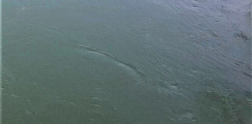
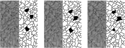
Region 3 in Fig. 1 is the portion of the graph characterized by the dominance of gravitational effects. This region is important because it is the most common region observed in rivers, streams and oceans. Therefore, a majority of terrestrial water flows can be located inside this region. As the surface deformations are small, it is assumed that this region can be described by linearized boundary conditions. Observing the surface in detail allows a wide number of local features to be recognized, such as waves, dimples (Fig. 2) and scars (narrow free-surface depressions generated by ascending vortex pairs and composed by whirls; Sarpkaya, 1996; Fig. 3). These features are caused by turbulence with enough energy to disturb the air–water interface, but only at scales smaller than the generating eddies dimensions. These small features can eventually evolve and break locally, leading to air entrainment.

Figure 2 Vortex dimples observed on the Donaukanal in Vienna, Austria, March 2019

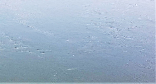
Figure 3 A scar observed on the Donaukanal in Vienna, Austria, March 2019

Regions 0 and 3 are relevant for typical shallow flows such as rivers and open channels. However, as acknowledged by Brocchini and Peregrine (2001), real flows can rarely be associated with a single point on the graph, but are best represented by trajectories that take into account the varying level of turbulence. The analysis presented in Brocchini and Peregrine (2001) was mainly qualitative as few experimental data were available to test their conceptual framework. Nonetheless, it serves as a useful framework to identify where further experimental studies are required.

3 Mechanisms driving the deformation of the free surface

The principal mechanisms that cause specific characteristics of the free-surface wave pattern (ensemble of surface features comprised of waves and other characters, e.g. dimples and scars) of turbulent flows have not yet been clearly identified. Some processes are thought to create patterns at the air–water interface, but they have not yet been sufficiently confirmed by experiments. A possible reason for this is the lack of experimental studies where both the bulk flow and the air–water interface behaviour were simultaneously measured with high enough accuracy and resolution. In order to develop better understanding of the free-surface behaviour, an examination of possible processes that may cause specific deformations of the free surface of a turbulent flow is given here. Such processes are: water surface interaction with coherent turbulent structures, resonance phenomena and effects of bed topography.

3.1 Impact of coherent structures onto the water surface

It is helpful to consider the definition of a coherent structure. According to Nezu and Nakagawa (1993), turbulent components in a flow are not independent from each other or completely random, but they demonstrate an organization in space and time. Such correlation gives rise to the concept of a “parcel” of fluid that has its own life cycle and that can be described as “coherent”. Several well-documented features fit with this definition, such as eddies, boils, horseshoe vortices and streaks. They generally divide into two types of coherent structure: bursting phenomena and large-scale vortical motions.

Bursting phenomena occur in the wall region and were discovered by Kline et al. (1967), Corino and Brodkey (1969) and Grass (1971). These phenomena were also described in detail by Rashidi (1997) for the smooth bed case. Near the bed, the sublayer structure is composed of alternating low and high-speed streaks that are induced by shear. Together with streaks, quasi-streamwise vortices form, straddling the low-speed regions. These vortices are present as single structures or in pairs, appearing as a hockey stick or horseshoe (Fig. 4). Once developed, the near-bed streaks and vortices begin to oscillate vertically due to the interaction with higher momentum fluid present in the overlying bulk flow. Subsequently, these structures disintegrate through a complete or partial breaking, forming groups of ejections (Rashidi, 1997). The remaining ejected fluid is then swept away by higher-momentum fluid of the bulk flow (Corino & Brodkey, 1969). The entire series of processes forms a “bursting phenomenon”. Over a rough bed the viscous sublayer is disrupted by the bed roughness; nonetheless streaks can still appear and evolve into bursts. This suggests a burst is not triggered by the instability of the viscous sublayer, but by the high-momentum fluid moving from the bulk region towards the bed (Nezu & Nakagawa, 1993). Support of the hypothesis can be found in Rashidi (1997).

Figure 4 Conceptual model of the creation and development of near-wall bursting phenomena that lead to the formation of boils at the free surface. (Reprinted from Rashidi (1997), Burst-interface interactions in free surface turbulent flows. Physics of Fluids, 9(11), 3485–3501, with the permission of AIP Publishing)

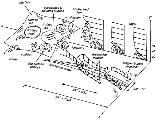
Large-scale motions have been described by Matthes (1947) and, differently from bursts, they may be present also in the outer region. Nezu and Nakagawa (1993) defined six different types of large-scale motions, but only one of these can be considered turbulence-related because it displays sufficient intermittency and randomness in space and size, while the others are just pulsations of the mean flow (low-frequency motions containing fine turbulence) (Nezu & Nakagawa, 1993). This turbulent motion was called a “kolk” by Matthes (1947), and it consists of a strong upward vortex that rises towards the surface and impacts on it, generating a boil (local raising of the free surface where the water flows out radially on top of the flowing prism (Matthes, 1947), also known as surface-renewal eddies; Fig. 5). Three forms of kolk-boil mechanism exist: “boils of the first kind” are produced by the flow separation downstream of bedforms (therefore they cannot occur over flat beds); “boils of the second kind” are related to secondary motions in the flow; and “boils of the third kind” are linked to bursting motions.

Figure 5 Boils observed on the Shinano River near Ojyia, Japan, April 2019

The first kind of boil was initially studied by Matthes (1947) and Znamenskaya (1963), and then by Jackson (1976). This form of boil has the tendency to form downstream of a bed feature in the lee area, where adverse pressure gradients form. This is supported by Kline et al. (1967) who noticed stronger and more frequent events for positive pressure gradients conditions.

Secondary motions are defined as a flow in the spanwise direction. As pointed out by Nezu and Rodi (1985), this motion weakens for high aspect ratios, i.e. the ratio between width of the channel and water depth, therefore it is not expected to appear in wide rivers. Nonetheless, turbulent velocity components allow the formation of unsteady turbulent secondary flows also for rivers with high aspect ratios. Secondary flows are associated with boils of the second kind. Boils of the second kind were studied by Imamoto and Ishigaki (1985), and by Tamburrino and Gulliver (2007). This form of boil is the result of slow-moving repeating patterns of vertical vortices, also known as streets, alternated with fast moving areas without disturbances (streaks). Tamburrino and Gulliver (2007) suggested that these streets are the manifestation of large streamwise vortices and outer region bursts: while bursts advect, they are trapped and channelled towards the free surface by the streamwise vortices, giving rise to upwellings (rising flows) and producing streets of vortices. By contrast, fast moving streaks originate in the areas where downwellings (descending flows) occur, so that bursts cannot reach the free surface.

The generation and development of the third kind of boil can be described using the conceptualization of Rashidi (1997) which is displayed in Fig. 4. Near-bed ejections, characterized by low momentum, move fluid upwards towards the free surface and generate spanwise “upsurging vortices” (kolks). Such upsurging vortices then rise towards the free surface and impinge on it, causing positive local increases in the instantaneous water height (boils). After the impact, the vortices fall back towards the bed and become “downswinging vortices” that produce reductions in the surface elevation (downswings). Quasi two-dimensional surface vortices which resemble whirlpools are then generated in the plane of the surface along the edges of the boils (Kumar et al., 1998). These vortices have been suggested to originate from surface deformations due to differences in the surface velocity between the boil and downswing areas (Pan & Banerjee, 1995).

It has to be noted that not all the bursts evolve into a boil. Grass (1971) found that not all the bursts cross the turbulent boundary layer and so only the most energetic are able to reach the free surface. Furthermore, in less energetic conditions a “blockage layer” exists close to the free surface which constrains the vertical component of turbulence and forces the redistribution of the turbulent kinetic energy (TKE) to the orthogonal directions (Longo, 2010). As a consequence, the free surface is barely perturbed (Smolentsev & Miraghaie, 2005). These two reasons might explain the longer periodicity of the boils compared to the bursts’ one than was observed by Narahari Rao et al. (1971). However, in strong turbulence situations, the blockage layer is thinner and the transfer of TKE is less effective, and so the water surface may be strongly deformed and broken into drops. This corresponds with the observations made in the numerical study by Zhang et al. (1999).

3.2 Excitation through resonance

Gravity-capillary wave theory describes the behaviour of the free surface of an incompressible fluid without viscosity, under the restoring effects of gravity and surface tension. A weakly deformed surface can be approximated as a linear combination of mutually independent sinusoids (waves). Each wave is characterized by a frequency, f, and by a wavenumber vector k with modulus $k=2\text{π}/\lambda$, where λ is the wavelength. The wavenumber vector is pointing in the direction of propagation of the wave, while the wave celerity is the ratio between the frequency and wavenumber modulus, $c=2\text{π}f/k$. The celerity of gravity-capillary waves is a function of the wavenumber, as well as of the flow depth, and mean flow velocity distribution. The relation between frequency and wavenumber is a dispersion relationship. Assuming a horizontally homogeneous flow, and no external forcing, the dispersion relation of gravity-capillary waves was obtained either analytically or numerically for a variety of average velocity vertical profiles, including a linear profile (Bièsel, 1950), power-function profile (Fenton, 1973), or more generic profiles (Ellingsen & Li, 2017). If the flow shear-rate is small (Shrira, 1993), the wave frequency can be approximated as: (2) $\begin{array}{rl}2\pi f\left(k\right)& =\mathit{k}\cdot {\mathit{U}}_0\pm k{c}_i\left(k\right)\\ & =\mathit{k}\cdot {\mathit{U}}_0\pm k\left[\right(g/k+Tk/{\rho }_f\left)\text{tanh}\right(kD){]}^{1/2}\end{array}$(2) where U₀ is the flow velocity vector at the surface, c_i(k) is the intrinsic celerity and D is the water depth. The two solutions with opposite signs represent waves with opposite direction of propagation. The intrinsic celerity c_i(k) in Eq. (2) indicates the speed of propagation of the waves relative to the mean flow. For water with depth larger than 2(T/ρ_fg)^1/2 = 5.5 mm, c_i(k) has a minimum of approximately 0.23 m s⁻¹ when the effects of gravity and surface tension balance, at λ ≈ 1.7 cm (k ≈ (ρ_f g/T)^1/2 = 367 m⁻¹). Longer waves are governed by gravity and have a maximum celerity limit of (gD)^1/2.

Waves of finite amplitude can grow from initially infinitesimal perturbations even when forcing mechanisms are weak, because of resonances (Brocchini & Peregrine, 2001). The resonance occurs when the speed of a disturbance matches the celerity of free waves. Considering a disturbance within the flow, at height z, which propagates parallel to the flow at the time-averaged local speed U(z), where 0 < U(z) < U₀, the condition for resonance is: (3) $U\left(z\right)=U_0+c_i\left(k\right)/\text{cos}\left(\theta \right)$(3) where θ is the angle of propagation of the wave with respect to the flow direction. Only waves that propagate against the flow (θ < 0) can be resonant, and only if U₀ > 0.23 m s⁻¹. For a given wavenumber k, Eq. (3) determines the height z, called the critical layer depth, where the resonance is possible. Depending on the nature of the disturbance and the characteristics of the velocity profile at the critical layer, the surface can become unstable, leading to wave growth. The mechanism, called shear instability or critical layer instability, has been the subject of numerous theoretical and numerical studies (e.g. Caponi et al., 1991; Morland et al., 1991; Yih, 1972; Young & Wolfe, 2014), but has not been validated experimentally yet for the case where the sheared fluid is below the surface.

Another case of resonant wave growth, distinct from the shear instability but still requiring the existence of a critical layer (hence of shear), was analysed numerically by Teixeira and Belcher (2006). The disturbance was represented by an initially homogeneous turbulent pressure field, which interacted with the free surface of an infinitely deep constantly sheared flow according to a rapid distortion formulation. During the initial stages of its evolution, turbulence was found promoting the resonant growth of free waves with the same celerity and wavelength of the pressure fluctuations, while it redistributed its energy across directions and scales as it approached the surface. The stabilization of the wave amplitude in some simulations was interpreted by Teixeira and Belcher (2006) as evidence of forced waves, which could not satisfy the resonance condition based on their free wave dispersion relation, but were instead forced to follow the speed of the pressure disturbance, c(k) ≈ U(z).

Considering Eq. (3) and the existence of a minimum of c_i(k), the location of a critical layer is confined between the bed and a maximum height z, where U₀ – U(z) > 0.23 m s⁻¹. For typical velocity profiles encountered in subcritical open channel flows, the surface-relative velocity U₀ – U(z) is small in the upper half of the flow, and the critical layer is relatively far from the surface, close to the bed. This means that resonant pressure and free-surface fluctuations must be distant from each other, which limits the strength of their interaction. For a constant U₀, a shallower depth gives a smaller distance of the critical layer from the surface. Similarly, as the flow surface velocity increases, the critical layer rises towards the surface, and a broader spectrum of waves can satisfy the resonance.

3.3 Influence of the bed topography

The appearance of waves at the surface of a flow over topography has been studied extensively, also beyond linear theory, but mostly limited to the steady case, with localized topography, and for an irrotational flow. A comprehensive review of these studies can be found in the work of Akselsen and Ellingsen (2019). The model presented in this work is probably the first to apply to a flow with a power function velocity profile and small but arbitrary three-dimensional bathymetries, although limitedly to linear waves. A small bed roughness shape can be seen as a perturbation of an otherwise flat, smooth bed. Similarly to a pressure perturbation, the bed can excite waves with a range of wavelengths and directions of propagation, including forced evanescent waves and free resonant waves (Harband, 1976). The disturbance is located where U(z) = 0, therefore the resonant waves must be fixed in time, and have frequency f = 0. This is possible if the waves propagate against the flow at the same speed at which they are advected. From Eq. (3) we have: (4) $c_i\left(k\right)=-U_0\text{cos}\left(\theta \right)$(4) These waves are called stationary waves, or sometimes (e.g. Rayleigh, 1883) standing waves.

A solution of Eq. (4) exists only when U₀> 0.23 m s⁻¹, and it appears as a specific relation between wavenumber and angle of propagation. When the bed disturbance is localized in space, the combination of all waves that satisfy this relation produces a characteristic wake-pattern in the far-field, similar to the one produced by a moving ship. Wakes are typically observed in rivers behind submerged (e.g. boulders, rocks) or surface penetrating obstacles (bridge piers). When the bed roughness is homogeneous, stationary waves can combine incoherently without producing a recognizable wake.

Stationary waves have been observed for a wide range of bulk Froude numbers (F = Ū/(gD)^1/2 = 0.3–3, where Ū is depth- and time-averaged mean flow velocity), over smooth and rough beds, and have been associated with spatial variations of the bed shear stress and formation of three-dimensional bedforms in movable-bed channels (Chanson, 2000). A few useful relations to estimate the wavelength and amplitude of stationary waves have been reviewed by Chanson (2000). For a given surface velocity, the stationary wave with the largest wavelength is the gravity wave with the crest perpendicular to the flow, with θ = 180°. For this wave to form, 0.23 m s⁻¹ < U₀ < (gD)^1/2, i.e. the flow must be subcritical. The wavelength of such a flow-perpendicular stationary wave, λ₀, can be calculated for a power-function velocity profile U(z) ∝ zⁿ (where n is the exponent of the power-function) as (Dolcetti & García Nava, 2019b): (5) ${\lambda }_0/D=2\text{π}{{\mathsf{F}}_{\mathsf{0}}}^2\left\{\left[I_{-\left(0.5+n\right)s}\left(2\text{π}D/{\lambda }_0\right)\right]/\left[I_{\left(0.5-n\right)s}\left(2\text{π}D/{\lambda }_0\right)\right]\right\}$(5) where F₀ = U₀/(gD)^1/2 is the Froude number based on the free-surface velocity, I_φ is a modified Bessel function of the first kind of degree φ, and s = sgn(0.5 – n) is the result of the sign function. A simpler form of Eq. (5) can be obtained assuming short (relative to the depth) waves and a profile with constant shear equal to n, U(z) ∝ nz, as (Teixeira, 2019): (6) ${\lambda }_0/D=2\pi {{\mathsf{F}}_{\mathsf{0}}}^2/(1+n{{\mathsf{F}}_{\mathsf{0}}}^2)$(6) Equations (5) and (6) will be used in the next section to compare with experimental observations of stationary waves in shallow flows.

4 Free-surface behaviour of open channel shallow turbulent flows

In the following section, a review of the literature that explores the observation of free-surface behaviour in open channel flows is given. There have been a limited number of studies which presented simultaneous measurements of the surface shape and flow field. This lack of data hindered the possibility to uniquely identify the mechanism that governs the free-surface deformation. Instead, most published works focused on determining the celerity (speed) of the patterns of surface deformation as it has a direct implication for non-contact flow velocity measurements. The speed of the patterns was also interpreted as an indicator of the dominant surface-generation mechanism under the assumption that turbulence-induced surface deformations move at the same speed (near-surface velocity) of the turbulent structures that caused them. The studies in this section have been grouped into three themes according to the underlying hypothesis about the governing surface-deformation mechanism. These themes mirror the three processes described in the previous section, i.e. the impact of coherent structures on the free surface, wave resonant growth and dominance of bed interaction, respectively. As we argue in the discussion, these hypotheses may have influenced the choice of the analysis as well as the way the results were interpreted, leading to some contrasting conclusions.

4.1 Interactions of coherent structures with the free surface

Turbulence-induced waves are a form of surface pattern that originates from the impact of turbulent coherent structures from below. The earliest experimental studies on the free surface of open channel flows were given in Freeze et al. (2003) and Smolentsev and Miraghaie (2005) and they were focused on supercritical flows. In these studies, the free-surface behaviour was described for conditions ranging from an almost undisturbed to a highly agitated free surface. Here, large Froude numbers were obtained using very steep flume slopes.

Important changes in the frequency and amplitude characteristics of the instantaneous water depth, obtained with an ultrasound transducer, were observed by Freeze et al. (2003) and Smolentsev and Miraghaie (2005) as the hydraulic conditions were changed towards the stronger turbulent regimes. Freeze et al. (2003) also observed that the probability density functions of the instantaneous water depth were well approximated by a Gaussian fit. Power spectral density plots of the fluctuating flow depth showed for both studies large peaks at low frequencies. Smolentsev and Miraghaie (2005) attributed these peaks to roll waves with wavelength longer than the flow depth, followed by a long tail of low period features that were associated with turbulence–surface interactions and with short gravity and capillary waves. Larger contribution of the shorter scales in the power spectrum and larger standard deviation of the depth were observed with an increase of the Froude number, indicating rougher water surfaces. Freeze et al. (2003) also found a weak dependence of the depth standard deviation on the flow Reynolds number.

Smolentsev and Miraghaie (2005) used halogen bulbs installed above the flow to project the free-surface wave patterns onto a white sheet placed on the bottom of the flume. The rise and fall of the free surface produced cellular patterns on the flume bottom, as shown in Fig. 6. The average cell size at the free surface decreased with the Froude number and turbulence intensity. Their advection velocity was found to be a few per cent above the mean flow velocity. The origin of these features was then associated with the disturbances of the free surface produced by turbulent events, e.g. eddies generated in the near-wall region, moving upwards and advecting at the mean flow velocity. Assuming a link between the characteristics of cells and the size of turbulent eddies, a different evolution of turbulent eddies while approaching the free surface was suggested in the case of weak or strong turbulence. For the weak turbulence case, the free surface behaves similarly to a rigid boundary and eddies evolve into two-dimensional structures similar to pancakes. In strong turbulence regimes eddies are able to maintain the original three-dimensional form and so to create larger surface deformations.

Figure 6 Time sequence of the observed and reconstructed free-surface cells. (Reprinted from International Journal of Multiphase Flow, 31(8), Smolentsev & Miraghaie, Study of a free surface in open-channel water flows in the regime from “weak” to “strong” turbulence, 921–939, Copyright (2005), with permission from Elsevier)

One of the few experiments in which the water surface and velocity field were measured simultaneously was presented by Fujita et al. (2011). Profiles of the free surface on the central plane of a channel were imaged at different instants in time, and then cross-correlated. From the time lag that showed the maximum correlation and the spacing between the observed positions Fujita et al. (2011) calculated the mean velocity of the water surface profile. They measured the flow velocity at the surface via the visualization of floating tracers which were released upstream. Comparisons between the fluctuating water surface elevation and vertical velocity components of turbulence showed that local increases in the water depth almost coincided with local peaks of the vertical velocity fluctuations. These surface features were then deformed during their advection with a speed similar (within an error of less than 10%) to the near-surface velocity. This suggested that the surface patterns could be used as indicators of the free-surface velocity. Correlations between water surface fluctuations and depthwise vertical velocity fields were positive near the surface and negative towards the bottom, and generally smaller than 0.15. This pattern of the measured correlation function suggested the existence of a vortex rotating in a clockwise direction at the intermediate depth, which tended to move towards the surface, interact with it and induce a local water rise together with a counter-clockwise whirl near the air–water boundary. Like the surface disturbance, the vortex structure was seen to travel with a speed comparable to the flow velocity at the surface.

A series of laboratory experiments with a rough bed channel were reported by Horoshenkov et al. (2013). Using a non-equidistant array of wave probes, the authors compared the speed of the surface roughness pattern with that of gravity-capillary waves generated artificially either in the presence or absence of flow (Eq. 2). The collected experimental data for several gravity-driven free-surface flows did not follow the dispersion relation of gravity-capillary waves but showed a propagation speed for the surface features between the surface velocity and the mean flow velocity, and independent of the wave frequency. This suggested a connection between the advecting surface pattern and the underlying turbulent structures. Because the free-surface pattern varied continuously in time and space, the authors studied its behaviour using a spatial correlation function that described the statistical and spectral characteristics of the dynamic surface. This function was found to flip sign as the spatial lag ρ increased. It was shown that for subcritical laboratory flows the spatial correlation function W(ρ) was approximated by a mathematical expression that combines a periodic function with an exponentially decaying term: (7) $\mathsf{W}\left(\rho \right)=\text{exp }\left(-{\rho }^2/{{\sigma }_w}^2\right)\text{cos}\left(2\pi \rho /L_0\right)$(7) where σ_w is the correlation radius, a measure of the correlation length of the surface pattern, and L₀ is the characteristic spatial period in the wave pattern observed on the free surface.

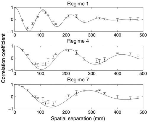
With a proper choice of the two parameters σ_w and L₀, Eq. (7) was able to approximate well the measured spatial correlation function, as shown in Fig. 7 for three different flow conditions. For all the hydraulic conditions examined by Horoshenkov et al. (2013), the two parameters were estimated using an optimization process. Horoshenkov et al. (2013) also demonstrates that the correlation radius, non-dimensionalized with the equivalent hydraulic roughness (capacity of the flow in dissipating energy), varied approximately linearly with the bulk Reynolds number, R_e = ŪD/ν. This suggests that the dissipation of the water surface waves is linked to the energy dissipation within the turbulent flow. Non-dimensionalizing the spatial correlation period with the bed roughness height made it possible to identify a clear nonlinear relation with the ratio of depth-averaged flow velocity to shear velocity, meaning that L₀ incorporates information on the shape of the vertical velocity profile. Finally, the characteristic spatial period was found to increase with the Froude number.

Figure 7 Measured and fitted spatial correlation function for progressively higher Froude numbers (F = 0.29, F = 0.54, F = 0.58 for regimes 1, 4 and 7, respectively). (Horoshenkov et al., 2013)

Nichols et al. (2016) further examined the oscillatory behaviour of the free surface observed by Horoshenkov et al. (2013) and proposed a model for the surface response to the turbulence-generated disturbances. The authors studied the characteristic spatial period L₀ in Eq. (7) as a function of the free-surface velocity, U₀, to define a characteristic frequency of oscillation of surface features, f₀: (8) $f_0=U_0/L_0$(8) They found that the free-surface behaviour excited by underlying turbulence undergoes an underdamped simple harmonic motion, where the surface pattern inverts periodically in time during the advection. The authors hypothesized that each discrete surface disturbance, once formed, oscillates around the mean water level while gravity and surface tension attempt to restore the equilibrium, therefore behaving like a spring and mass system. Meanwhile, gravity waves that travel outward in all directions are likely to be generated. Their hypothesis implies that the complex surface pattern may be considered as an ensemble of “oscillons” that overlap in space and time, maybe out of phase. Neglecting the effect of surface tension, Nichols et al. (2016) proposed a simple equation which relates the characteristic frequency of a simple harmonic motion of a water surface feature, f₀, to the root-mean-square of the water surface wave height, σ_RMS. 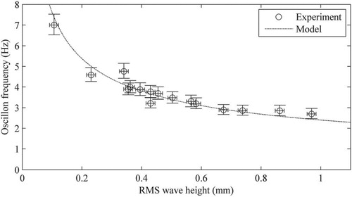This is expressed as: (9) $f_0=(2\pi {)}^{-1}\left\{g/\right[(1.5N+1){\sigma }_{RMS}]{\}}^{1/2}$(9) where N is a factor that represents the depth of influence, i.e. the relative vertical extent of the flow field which is affected by a surface deformation.

This model was validated against the data presented by Horoshenkov et al. (2013), for a range of experimental values of L₀ and U₀ (Fig. 8). Nichols et al. (2016) found that the values of the depth of influence factor, N, calculated by fitting the measured correlation functions, was relatively constant for a representative range of flow conditions, and equal to N = 28. This means that the free-surface displacements influenced the underlying hydrodynamics up to 28 surface height standard deviations below the mean water level. The model of Nichols et al. (2016) could explain the different linkages between the interface and the sub-surface turbulence that were observed in the past as different kinds of surface features (such as boils, dimples, etc.), that are produced by the turbulent structures, may be related to the phase of the oscillatory process of the free surface. It was further postulated that pressure fluctuations associated with the surface oscillations could be a factor in the generation of coherent flow structures near the bed. For this reason, the simple harmonic frequency was compared to the frequency of near-bed burst generation f_B, which was derived from Nezu and Nakagawa (1993) as: (10) $f_B=U_0/\left(N_{B}D\right)$(10) where N_B is the normalized bursting period that Nikora and Goring (2000b) claims to vary between 1.5 and 3.0. A mean value of 2.25 was found to give correspondence between f₀ and f_B, meaning that the oscillation period can be directly linked to the near-bursting period. Since there is a simply physical explanation for f₀, which does not depend on the flow or bed conditions, this suggests that surface oscillations trigger near-bed bursts through induced pressure fluctuations.

Figure 8 Comparison between the measured values (markers) of the surface oscillation frequency for different conditions and the modelled data (dashed line). (Nichols et al., 2016)

Attempts to validate the observations by Horoshenkov et al. (2013) and by Nichols et al. (2016) with field data have been described by Legleiter et al. (2017), and by Noss et al. (2019). Legleiter et al. (2017) created a model of the surface shape based on the theoretical correlation function of Eq. (7) proposed by Horoshenkov et al. (2013) and rescaled it in order to model the spatial distribution of sun light intensity reflected by the free surface of a river. However, the surface shapes predicted by such a model were found to be too wide and smooth compared to what was expected.

Noss et al. (2019) designed a floating instrument capable of recording its vertical acceleration as it followed a flow trajectory at the surface. The acceleration was then converted to a measure of the surface elevation in a Lagrangian frame, and its statistics were compared to parameters of the flow for a range of experiments in a laboratory flume and in a river. The Lagrangian elevation showed a strong quasi-sinusoidal fluctuation, as predicted by the theory of Nichols et al. (2016). Fitting the measured fluctuation frequency and amplitude with Eq. (9) proposed by Nichols et al. (2016), however, yielded somehow inconsistent values of the depth of influence parameter, N. Instead, Noss et al. (2019) identified approximately linear relations between the standard deviation of the drifter elevation estimated from the Lagrangian acceleration, and the flow velocity, bulk Froude number, and bulk Reynolds number. Noticeably, the surface statistical moments were found to correlate very well with the shear velocity, suggesting an apparent link between free-surface behaviour and hydraulic resistance.

A similar link had been previously suggested by Cooper et al. (2006), based on measurements of the surface statistics with an ultrasonic sensor. Observations and measurements from past studies (e.g. Buffin-Bélanger et al., 2000; Robert et al., 1996) indicated that large-scale structures govern the transfer of momentum and so the friction between the bed and the fluid. This encouraged Cooper et al. (2006) to propose that the dynamic behaviour of the surface is linked to the resistance imposed by the bed, i.e. that the spatial roughness properties of the bed control the bulk hydrodynamics and free-surface behaviour. The main finding was that a higher level of hydraulic resistance and lower water depth give rise to many small laterally elongated boils on the surface. Rougher water surfaces were dominated by fewer but larger renewal eddies for smaller hydraulic resistances and higher water depths. Around these boils the water was observed to be much flatter.

4.2 The importance of gravity-capillary waves

Savelsberg et al. (2006) published a study demonstrating a linkage between the free surface and the underlying hydrodynamics. In their study the free surface of the flow in a laboratory flume was defined via the space-time surface gradient field which was measured with a laser scanning technique. The reason behind the use of the free-surface gradient rather than its elevation was because the spectral energy of the latter decreases much more slowly than the former with an increasing wavenumber, therefore smaller features could be measured with higher accuracy. Turbulence in the flume was produced by means of an active grid. The underlying turbulent field was measured using particle image velocimetry (PIV) and laser-Doppler anemometry (LDA). Spatial autocorrelations at time-lag 0 of the surface gradient were seen to decrease rapidly with the spatial lag, especially in the transverse direction, and to fluctuate between positive and negative values, in agreement with Horoshenkov et al. (2013). Time series of the surface roughness gradient in the spanwise direction enabled Savelsberg et al. (2006) to investigate the Taylor’s frozen turbulence hypothesis, i.e. whether or not a time-dependent signal of a one-dimensional space measurement of the free surface in this type of flow can be used to reconstruct the whole spatial domain of the surface at a given moment. Analysis of the space-time correlation function of the free-surface gradient suggested that the hypothesis is not valid for the free surface above a turbulent flow, although it works well for the velocity field beneath the free surface. This was explained by the presence of gravity-capillary waves that Savelsberg et al. (2006) associated with the turbulent velocity field beneath the surface as the wavelength of the surface waves was close to the integral scale of the turbulent velocity.

Continuation of this work was presented by Savelsberg and van de Water (2008), with the aim of defining the strength of the correlation between the surface and the underlying turbulence. In their experiments only small deformations of the free surface were observed, mainly shallow and rounded wrinkles, despite the active grid generating relatively strong turbulence. The free-surface gradient was correlated with the normalized convective acceleration, (u · ∇)u, where u is the turbulence velocity vector. The correlation function for the fully developed turbulent free flow condition was found to be small (0.04). The absence of a strong correlation between the gradient of the free surface and the underlying turbulent velocity field led Savelsberg and van de Water (2008) to conclude that the interface possesses independent dynamics. The convective acceleration was then separated into two terms representative of strain and rotation and correlated with the surface gradient field. For the fully developed turbulent flow, the strain correlation was twice that of the rotation correlation, meaning a predominance of upwellings and downwellings compared to vertical vortices. The energy spectrum of the surface gradient showed patterns travelling at the mean flow velocity with relatively low wavenumbers. However, they were outweighed by different features which approximately satisfied the dispersion relation for gravity-capillary waves. The wavelength of the gravity-capillary waves was comparable to the longitudinal integral length scale of the sub-surface turbulence field. This suggested that the free surface was mostly excited by the largest sub-surface turbulence scales. Spatial correlation of the streamwise and spanwise surface gradient at different locations were seen to be isotropic when the turbulence was isotropic, and anisotropic when turbulence was the same. In conclusion, Savelsberg and van de Water (2008) found that the surface was dominated by gravity-capillary waves and that the free surface inherits from the sub-surface turbulence the lower wavenumber properties of integral length scale and anisotropy, while for higher wavenumbers the surface has a behaviour independent from the turbulence field.

This research was then extended in 2009 to both active and static grid turbulence by Savelsberg and van de Water (2009). They discovered that the amplitude of surface gradient fluctuations is correlated with the turbulent Reynolds number. A steep wavenumber spectrum proportional to k⁻⁶ was observed for the free-surface gradient. They also discovered that the phase velocity along the spanwise direction has a small dependence from the Reynolds number for the active grid case. Finally, they observed non-proportionality between the length scales of the surface gradient and the integral scales of the sub-surface turbulence for the two cases of active and passive grids, probably caused by the different manner of stirring.

Image-based methods rely on the hypothesis that the surface patterns are advected downstream with the surface velocity. However, surface textures can also be dispersive, i.e. patterns of different scales propagate at different speeds if gravity-capillary waves are present. Therefore, significant errors are likely to occur in the surface velocity estimations which are based on such a hypothesis. Tani and Fujita (2018) analysed space-time images (STI) (Fujita et al., 2007; Fujita & Tsubaki, 2002) of orthorectified (corrected so that the central perspective of the object is restored and a single scale of reference for the entire image holds) flow videos of the surface or actual rivers. They computed the Fourier transform in space and time of these data, to estimate the frequency–wavenumber spectra of the surface elevation. From it, they discovered that the major part of the energy was distributed among the dispersion relations of both turbulence and gravity-capillary waves. Filtering the data to remove the gravity-capillary wave components enabled them to improve significantly the accuracy of the velocity estimated with the STI method.

4.3 Stationary waves as primary components in the free-surface patterns

A Fourier analysis similar to the one implemented by Savelsberg and van de Water (2009) was applied by Dolcetti et al. (2016) to two orthogonal arrays of calibrated wave probes installed in a laboratory flume with the bed formed with regular spheres with the diameter of 25.4 mm. The frequency–wavenumber spectra of the surface elevation were interpreted based on a linear wave model derived for a power-function velocity profile by Fenton (1973), extending a previous result by Burns (1953). The larger measurement area compared to the experiments of Savelsberg and van de Water (2009) allowed the behaviour of longer waves to be identified more clearly. Whenever the necessary condition for their occurrence (U₀ > 0.23 m s⁻¹) was met, stationary waves were clearly identified by a peak of the frequency–wavenumber spectrum at f = 0. While Eq. (4) allows waves with different combinations of wavenumber and direction to be stationary, the only stationary waves that could be observed had their front perpendicular to the direction of the flow, and their wavelength was predicted well by Eq. (5). These stationary waves were found to be the dominant feature of the surface fluctuation, despite the lack of localized obstacles at the bed. They had a direct effect on the spatial correlation of the surface elevation, which was found fluctuating in space as observed by Horoshenkov et al. (2013), but with the wavelength λ₀ instead of L₀.

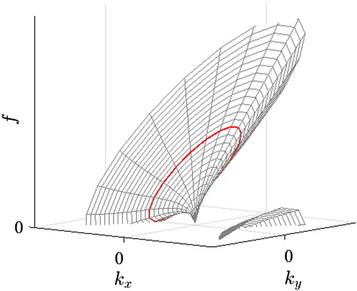
The frequency–wavenumber spectra measured by Dolcetti et al. (2016) (Fig. 9) show a concentration of energy along specific lines (an almost straight line in the streamwise spectrum, and an ellipse in the lateral spectrum). These lines correspond approximately to the projections of the ellipse indicated in red in Fig. 10, which represents the dispersion relation of waves with constant wavelength λ₀, and with θ that varies in all directions. Defining k₀ = 2π/λ₀ as the wavenumber of the stationary wave with wavelength λ₀, the frequency of these waves is found from Eq. (2) and Eq. (4) as: (11) $f\left(k_0\right)=k_0{U}_0[1+\text{cos }(\theta \left)\right]=(k_0+k_x)U_0$(11) where k_x is the streamwise component of vector k₀. When θ = π, then f (k₀) = 0, and the wave is a stationary wave. When θ ≠ π, the gravity-capillary waves are freely propagating and f (k₀) > 0. Similar patterns in the spectra could not be seen for the flow condition with U₀ < 0.23 m s⁻¹, when stationary waves could not form. In this case, the forced waves that moved at the mean flow velocity were seen together with freely propagating gravity-capillary waves. Acoustic measurements by Dolcetti et al. (2017) suggested that forced waves can still be present (at least in the capillary range) alongside stationary waves, and that their amplitude increases faster with the increasing Froude number than the amplitude of free waves; a result later contradicted by Yoshimura and Fujita (2020) by means of a direct numerical simulation. The Froude number was also found decreasing the steepness of the surface frequency spectra by Dolcetti et al. (2016), suggesting a relatively high contribution of shorter scales (therefore a rougher water surface) at higher Froude numbers. Like Savelsberg and van de Water (2009), Dolcetti et al. (2016) explained the presence of forced waves invoking the mechanism described by Teixeira and Belcher (2006). However, the predominance of stationary waves in the faster flow conditions, and the scaling of the correlation function and of the dynamic surface fluctuations with the wavelength λ₀, suggested a stronger role of the bed topography than previously thought.

Figure 9 Streamwise (left) and spanwise (right) non-dimensional frequency–wavenumber spectra for the case U₀ > c_min. Frequency and wavenumber were non-dimensionalized using the wavenumber of the stationary wave, k₀. The contours have been non-dimensionalized to compensate for the decay with frequency. (Reprinted from Dolcetti, Horoshenkov, Krynkin, & Tait (2016). Frequency-wavenumber spectrum of the free surface of shallow turbulent flows over a rough boundary. Physics of Fluids, 28(10), 105105, with the permission of AIP Publishing)

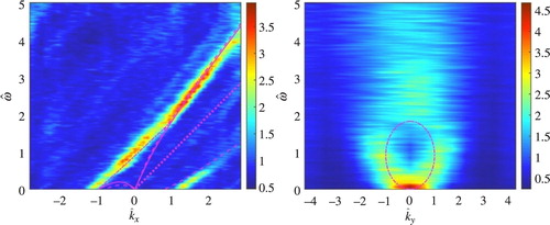
Figure 10 Representation of the three-dimensional dispersion relation shell (Eq. 2). k_x and k_y are the components of the wavenumber vector in the streamwise and lateral directions, respectively. The two surfaces represent the two solutions for upstream and downstream propagating waves. The red line indicates the frequency of the waves with wavelength λ₀ for different directions of propagation

A more detailed view of the same stationary wave related surface patterns was obtained by Dolcetti and García Nava (2019a), with a wavelet-based analysis of the same dataset. The wavelet-based analysis provided a better three-dimensional representation of the frequency–wavenumber spectra, confirming the free-surface behaviour suggested by Dolcetti et al. (2016). It also allowed quantification of the angular spectrum of the waves with wavenumber k₀. Applying the framework suggested by Legleiter et al. (2017), Dolcetti and García Nava (2019a) proposed a simplified surface model based on an inverse Fourier transform of a surface spectrum, S_S(k, θ), described by: (12) $S_S\left(k,\theta \right)\propto \text{exp}\left\{b\left[\text{cos}\left(\theta -\pi \right)-1\right]\right\}\delta \left(k-k_0\right)$(12) where b is an angular distribution parameter which was found to be between 1 and 2, and δ is a delta-function that excludes all waves with wavelength different from λ₀ from the model. The model describes the free surface as a linear combination of freely propagating waves with the same wavelength λ₀ and with different direction of propagation. With it, Dolcetti and García Nava (2019a) were able to justify the fluctuation of the space-time correlation function observed by Horoshenkov et al. (2013). The model was further expanded by Dolcetti et al. (2020), yielding a series representation of the full spatial-temporal correlation: (13) $\begin{array}{rl}\mathsf{W}(\mathit{\rho },\tau )& =a_0{J}_0\left(k_0|\mathit{\rho }-{\mathit{U}}_0\tau |\right)\cos \left(k_0{U}_0\tau \right)\\ & +\sum _{\phi =1}^{\mathrm{\infty }}{a}_{\phi }(-1{)}^{\phi /2}\left[J_{\phi }\right(k_0|\mathit{\rho }-{\mathit{U}}_0\tau |)\text{exp}(-\text{i}{k}_0{U}_0\tau )\\ & +J_{\phi }\left(-k_0|\mathit{\rho }-{\mathit{U}}_0\tau |\right)\text{exp}\left(\text{i}{k}_0{U}_0\tau \right)]\end{array}$(13) where a_φ are the series coefficients that depend on the angular spectrum, and J_φ is the Bessel function of the first kind of order φ. This equation was used by Dolcetti et al. (2020) to interpret the autocorrelation of images of a shallow river surface, recorded by a camera. Like in the laboratory, the river surface slope spectra (Lubard et al., 1980) showed a similar pattern of waves with wavelength λ₀. The measured correlations showed similar fluctuations in space and time, which were matched by the behaviour of the trigonometric and Bessel functions in Eq. (13).

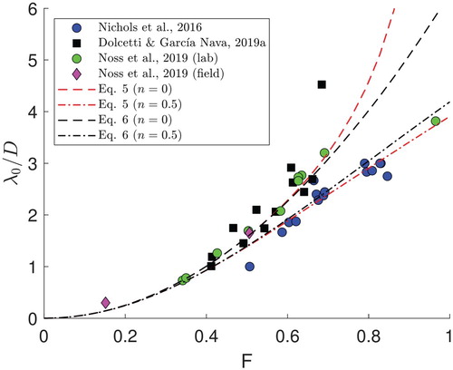
The model of Dolcetti and García Nava (2019a) predicts for an observer that moves along the flow at the mean surface flow velocity U₀ a periodic inversion of the surface shape, η, i.e.: (14) $\eta (x=U_{0}t,t)=A\text{cos}\left[k_0{U}_0\left(t-t_0\right)\right]$(14) where A is the wave amplitude and t₀ is the initial time step. This behaviour is similar to the one described by Nichols et al. (2016), who had predicted a fluctuation with frequency f₀ = U₀/L₀. The model could also justify the quasi-periodic fluctuations of a Lagrangian drifter, observed by Noss et al. (2019). According to the model of Dolcetti and García Nava (2019a) and to Eq. (14), if the drifter is assumed to travel approximately at the speed of the flow near the surface, U₀, then it should observe a periodic fluctuation with frequency k₀U₀/2π = U₀/λ₀. A comparison of the characteristic surface frequencies observed by Nichols et al. (2016) and Noss et al. (2019) with the one prescribed by the model of Dolcetti and García Nava (2019a) can be found in the works of Dolcetti and García Nava (2019a) and Dolcetti and Tait (2020, in press), respectively. Both results are summarized in Fig. 11, which compares the non-dimensionalized stationary waves wavelength λ₀/D (calculated via Eq. (5) and its approximation Eq. (6), for two velocity profile exponents, n = 0.5 and n = 0), with the corresponding equivalent wavelength observed by Nichols et al. (2016) and Noss et al. (2019), calculated from f₀ and L₀ as: (15) ${\lambda }_0/D=U_0/\left(f_{0}D\right)=L_0/D$(15) The same figure also includes the wavelength of the stationary waves calculated from the wavelet spectra measured by Dolcetti and García Nava (2019a). All three datasets showed an agreement with the theory (although for different velocity profile exponents), suggesting that stationary waves may control the scales of the surface deformation over a broad range of flow conditions, also in the field. This was interpreted by Dolcetti and García Nava (2019a) and Dolcetti and Tait (2020, in press) as evidence of a more general predominance of bed roughness forcing over turbulence, in contrast with previous works.

Figure 11 Non-dimensionalized dominant surface scale measured by Nichols et al. (2016), Dolcetti and García Nava (2019a), and Noss et al. (2019), compared to the wavelength of stationary waves predicted by Eq. (5) (power-function velocity profile) and Eq. (6) (constant-shear profile, short waves) with power-function exponent n = 0 and n = 0.5. The frequency values measured by Noss et al. (2019) have been converted to an equivalent spatial scale as λ₀= U₀/f₀. F is the bulk Froude number

Despite these observations, the mechanism that can cause the selective growth of waves with wavelength λ₀ not oriented against the flow, and hence not stationary waves, remains unclear. As a possible explanation, Dolcetti and García Nava (2019a) invoked a triad resonance mechanism originally proposed by Zakharov and Shrira (1990) to explain the broadening of the ocean spectrum in the presence of sheared oceanic currents. In principle, the mechanism allows the transfer of energy between a stationary wave, a freely propagating wave with the same wavelength, and a forced wave or a (turbulent) sub-surface flow perturbation. Resonant interactions among multiple waves require a deviation from linear theory, which appears to be justified by a weakly non-Gaussian probability distribution of the surface elevation (Dolcetti, 2017). However, measurements of the surface spectrum broadening are contradicting (Dolcetti & García Nava, 2019a), and the theory is based on assumptions that do not rigorously apply to shallow flows.

5 Discussion

The most interesting observation from the studies reviewed in this paper is concerned with the typology of wave patterns that dominate the free surface. More specifically, Fujita et al. (2011), Horoshenkov et al. (2013) and Nichols et al. (2016) state that these patterns are composed by turbulence-induced fluctuations. The hypothesis that gravity-capillary waves are the most relevant patterns is supported by Savelsberg et al. (2006), Savelsberg and van de Water (2008), Savelsberg and van de Water (2009), Dolcetti et al. (2016) and Dolcetti and García Nava (2019a). In particular, Dolcetti et al. (2016) and Dolcetti and García Nava (2019a) specify that these waves are stationary waves.

The theory of the turbulence-induced waves is supported by direct visualization (Fujita et al., 2011; Gharib & Weigand, 1996) of vortices impinging onto the free surface and creating local rises in the water depth. Using space-time images, Fujita et al. (2011) observed that the newly created surface features travelled at approximately the free-surface velocity. This mechanism for the free-surface pattern appears sensible as eddies increase their streamwise advection velocity while moving upwards until they reach the free-surface velocity. Wave patterns moving at the flow surface velocity were also observed by Horoshenkov et al. (2013) using an array of wave probes, by Nichols et al. (2016) via space-time images and by Tani and Fujita (2018) by means of space-time images and frequency–wavenumber spectrum. These observations suggest that after the impact of an eddy the free surface begins to oscillate according to the simple harmonic motion model described by Nichols et al. (2016). The complex free-surface pattern can be explained as a superposition of different single surface responses occurring in many points in space and out of phase. It was suggested by Nichols et al. (2016) that these features continue to oscillate while being advected downstream until they are dissipated by viscosity or are superseded by new surface features. According to Nichols et al. (2016), these features (oscillons) can generate gravity-capillary waves that propagate in all the directions. Patterns advecting with the surface velocity and generated by the flow turbulence were observed also by Savelsberg et al. (2006) and Savelsberg and van de Water (2008, 2009). However, in these studies the authors claim that the importance of these features is secondary to the dispersive gravity-capillary waves. These dominant capillary waves propagate in all directions may be generated through a resonance mechanism different from the one suggested by Teixeira and Belcher (2006). Evidence supporting this is that the wavelength of the dominant gravity-capillary waves was close to the sub-surface turbulence integral scale but the turbulent velocity was an order of magnitude smaller than the minimum phase velocity. In the experiments carried out by Savelsberg et al. (2006), Savelsberg and van de Water (2008) and Savelsberg and van de Water (2009) turbulence was generated using active and passive grids (which is rather different to river flows where turbulence is primarily generated by the instabilities in the boundary layer near the rough bed), therefore the length scales will be differently scaled from that expected in gravity-driven open channel flows. The observations by Dolcetti et al. (2016) and Dolcetti and García Nava (2019a) suggest different free-surface pattern generation mechanisms occur according to the flow condition. When the free-surface velocity is slower than the minimum phase velocity for gravity-capillary waves in still water, c_min = 0.23 m s⁻¹, the dominant pattern is formed by waves induced by turbulence through the forcing non-resonant growth proposed by Teixeira and Belcher (2006). When c_min > 0.23 m s⁻¹ the free surface is dominated by stationary waves and freely propagating gravity-capillary waves travelling in all the directions with the same wavenumber k₀. The spatial period L₀ measured by Horoshenkov et al. (2013) and predicted by Nichols et al. (2016) by means of a semi-empirical formula can in fact be predicted well in terms of the wavelength of stationary waves with the analytically derived wavenumber k₀. Dolcetti and García Nava (2019a) suggested that the free-surface fluctuations observed by Horoshenkov et al. (2013) and Nichols et al. (2016) were not localized manifestations of turbulence, but gravity-capillary waves that were probably induced by an interaction between the rough bed and sheared current. Dolcetti and García Nava (2019a) suggested that stationary waves mediate the transfer of energy between propagating waves and turbulence modes, causing a selective growth of waves whose scale and velocity match the wavenumber k₀. Furthermore, in addition to the waves with wavenumber k₀, gravity-capillary waves with different wavenumbers and turbulence-induced wave patterns may also occur. The analysis of the wave patterns and their dispersion relations by Dolcetti et al. (2016) and Dolcetti and García Nava (2019a) was based on the time-space Fourier and wavelet transforms. One can argue that these are more robust techniques than the cross-correlation of temporal wave probe data used in earlier studies by Horoshenkov et al. (2013) and Nichols et al. (2016). Other studies based on Fourier analysis did not identify the presence of stationary waves. A possible reason for this is a limited spatial window of the measurements. In Savelsberg et al. (2006) and Savelsberg and van de Water (2008, 2009) the spatial extent for investigating the surface was 50 mm. In the study by Fujita et al. (2011) the length of the field of view was 135 mm. These spatial windows are rather limited given the fact that Dolcetti et al. (2016) reported the presence of strong stationary waves with wavelength ranging 85 to 100 mm for similar flow conditions. Also, even larger stationary patterns with wavelength between 70 and 180 mm were observed in experiments with characteristics close to the ones tested in Nichols et al. (2016) where the area of interest was 220 mm long. Considering Horoshenkov et al. (2013), Nichols et al. (2016) and Dolcetti et al. (2016) where similar flow conditions but different bed textures were tested, one might argue that a specific dominating mechanism for the wave patterns can occur according to the flow and bed morphological conditions. In Dolcetti et al. (2016) regular spheres with the diameter of 25.4 mm were used, while in the other two studies the mean grain size of the bed was 4.4 mm, implying that, for the same flow conditions, different submergences (the ratio between the water depth and the dimension of the bed roughness) were present. For this reason, the effects of the bed on the free-surface behaviour may be limited to only higher submergences, facilitating the dominance of the turbulence-induced features when the submergence is lower. However, the role of submergence is unclear, and results by different authors are contradicting. For example, the experiments in Fujita et al. (2011) and Nichols (2013), which were characterized by submergences that fall in the range of conditions tested by Dolcetti et al. (2016), resulted in a different free-surface behaviour. This suggests that it is not only the submergence that defines the type of response of the free surface but possibly the bed morphology itself. Meanwhile, according to Noss et al. (2019), the dynamics of the interface is sensitive to the submergence, being affected by turbulence for high values of submergence and showing stationary waves for small values of it. Therefore, no single dominating mechanism appears to govern the free-surface behaviour.

Despite different points of view, the majority of studies support the existence of a similar spatial organization for the free surface. Savelsberg et al. (2006) observed oscillating correlation functions for the instantaneous surface gradient and different behaviours between the streamwise and spanwise directions. Savelsberg and van de Water (2008) suggested that the spatial correlation behaviour depends on the turbulence field: it behaves isotropically if the turbulence is isotropic; or anisotropically if turbulence is anisotropic. Horoshenkov et al. (2013) provided an analytical description of the average spatial correlation function for the free-surface elevation (Eq. 7). This equation has a characteristic spatial period and decreases in amplitude with the distance. Its characteristics are related to the turbulence in the bulk flow. Dolcetti et al. (2016) observed for the case of mean surface velocity below 0.23 m s⁻¹ a smooth decay for the elevation correlation with horizontal scales approximately equal to the water depth. When the mean surface velocity is higher than 0.23 m s⁻¹ the correlations show a fluctuating behaviour with period defined by k₀.

The Taylor’s frozen turbulence hypothesis, which assumes that turbulence is invariantly advected in space at different time steps, was tested in Savelsberg et al. (2006) and it was found inapplicable at the free surface due to the appearance of gravity-capillary waves, but appropriate for the sub-surface velocity field. The violation of the Taylor’s hypothesis is further supported by the oscillon model of Nichols et al. (2016), which suggests surface features oscillate vertically over space and time, while the sub-surface structures persist as they are advected by the flow.

The free-surface roughness observations in Cooper et al. (2006) suggest that rougher surfaces are generated over a hydraulically rougher bed. Also, tests with low water depth and high bed resistance give rise to many small laterally elongated boils, while high water depth and lower hydraulic resistance produce less and larger features. Horoshenkov et al. (2013) noticed that the surface roughness height increases linearly with the water depth and the average velocity. In Nichols et al. (2016) rougher surfaces can be found for higher Froude numbers, but here the water roughness height was also a function of the bed slope. In Dolcetti et al. (2016) the characteristics of the surface were estimated from the frequency power spectra. They suggested that higher Froude numbers were linked to milder decays of the spectra at higher frequencies, i.e. that more energy was contained in these frequencies. As a consequence, rougher water surfaces should be seen for higher Froude numbers; however, no clear relation between the standard deviation of the surface depth and the Froude number was proposed. In Noss et al. (2019) the surface roughness was found to be more affected by the near-surface velocity, the Reynolds number and the shear velocity rather than the mean flow velocity. In particular, the shear velocity relation showed a high coefficient of determination not only in flume experiments, but also in real streams.

Figure 12 is a summary of key studies of the behaviour of free-surface pattern in open channel flows mapped onto the Brocchini and Peregrine (2001) framework (also see Fig. 1). The purpose is to demonstrate the range of laboratory and field measurements using the existing framework suggested by Brocchini and Peregrine (2001) and so indicate gaps in the available datasets in comparison to full scale conditions. The key parameters against which these data are plotted are the mean flow depth and turbulence velocity magnitude. Figure 12 was created using the following assumptions. Firstly, except for a few cases, the turbulent velocity component was taken as 7.5% of the bulk depth averaged velocity. This choice was made because in a majority of studies the streamwise turbulent velocity and the shear velocity were not observed or reported. The value of 7.5% is an approximate measure of the relative scale between the streamwise turbulent component and the bulk velocity for a range of smooth and rough bed cases as suggested by Nezu and Nakagawa (1993). Secondly, the horizontal axis is the water depth because the length scales of turbulence were not observed or estimated in a majority of studies reviewed. This choice is supported by Shvidchenko and Pender (2001) and Roy et al. (2004) who suggested that the vertical size of the turbulent macrostructures can grow up to the flow depth. Thirdly, the lines that subdivide the graph into four sections were calculated using the value of W_e,BP = 0.5 and F_BP = 0.155 (Eq. 1). These special forms of the indices correspond to F = 2.92 and W_e = ρ_f Ū ²D/T = 177.78 for the bulk Froude and Weber numbers, respectively. The adopted values of W_e,BP and F_BP yield to dividing lines which follow the same trends as shown in Brocchini and Peregrine (2001).

Figure 12 A summary of laboratory and field observations organised following Brocchini and Peregrine (2001). The streamwise turbulent velocity component was defined through the bulk velocity using the relations given in Nezu and Nakagawa (1993). Water depth scales with the largest size of a coherent structure. Black and grey dashed lines are obtained from Eqs. (3.1) and (3.2) in Brocchini and Peregrine (2001), respectively. Black and grey dotted lines define the separations between the regions and are obtained from Eq. (1) using F_BP = 0.155 and W_e,BP = 0.5, respectively. Black dashed-dotted line represents the condition R_e,BP = 100. (Brocchini & Peregrine, The dynamics of strong turbulence at free surfaces. Part 1. Description. Journal of Fluid Mechanics, 449, 225–254, 2001, modified with permission)

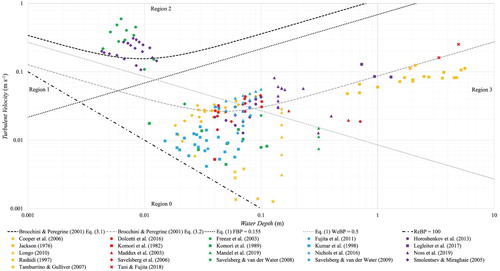
It is clear that field measurements cluster in region 3. This is consistent with findings by Brocchini and Peregrine (2001) who identified this zone as the most appropriate to describe a majority of the geophysical surface flows such as rivers and open channels. A majority of laboratory experiments fall in region 0 or near the border between region 0 and 3. The only exception is represented by the most energetic cases in Nichols et al. (2016). This means that the turbulent processes in most of the laboratory studies are relatively weak and may be non-representative of the large-scale geophysical flows. In fact, moving towards flow conditions which are more representative of a river is a challenge for laboratory studies. Higher mean flow velocities for a given flow depth are possible only by reducing the roughness height or by increasing the slope of a laboratory flume. The first possibility is in general not practically achievable as laboratory flume boundaries are not very rough. Testing deeper flow conditions for a given velocity is in most cases impractical as it would require much larger values of discharge. Furthermore, increasing the water depth causes a reduction in the aspect ratio and so the appearance of steady secondary motions. As a consequence, flow conditions that follow in region 3 are almost unexplored in laboratory studies. On the other hand, field measurements have much lower spatial and temporal resolution compared to laboratory instruments, making it difficult to accurately observe free-surface behaviour at a field scale. This, for example, may explain the discrepancy between the findings by Legleiter et al. (2017) (region 3) and by Horoshenkov et al. (2013) (regions 0 and 3). Also, field devices, such as mareographs and acoustic Doppler current profilers, are often invasive and so produce data that are not reliable when the interaction between surface and hydrodynamics is investigated. These reasons suggest that region 3, defined by Brocchini and Peregrine (2001) as the most representative of terrestrial flows, is almost unchartered.

6 Conclusions

This review suggests that the main question, “What controls the behaviour of the free surface?”, is yet to be conclusively answered. At present, three different hypotheses coexist, all supported by evidence from laboratory observations. They are: (i) turbulence-induced features, (ii) travelling gravity-capillary waves, and (iii) stationary waves. The main reason for this uncertainty can be attributed to either their different spatial and temporal resolutions or the inability of the measurement and analysis methods used to measure accurately these free-surface characteristics. Furthermore, the measurement uncertainties that arise in the study of the near surface region make it difficult to unambiguously couple the actual dynamics of the free surface and the underlying hydrodynamics. Despite the different outcomes of the reviewed studies, some agreement can be found:

• turbulence can affect the behaviour of the free surface over a wide range of hydraulic conditions, from those in which only small surface features are induced to conditions in which the surface can be fully broken (Brocchini & Peregrine, 2001);

• higher Froude numbers produce rougher water surfaces; in fact, more energetic conditions allow turbulent structures to maintain their original 3D form during the ascension towards the interface, resulting in larger surface deformations and leading to rougher free surfaces (Smolentsev & Miraghaie, 2005);

• the dynamic patterns on the free surface are shown to be correlated over space; it is suggested that this spatial behaviour can be approximated by a periodic, exponentially decaying function that contains information about the shape of the vertical velocity profile, bed roughness and turbulence energy dissipation rate (Horoshenkov et al., 2013);

A majority of studies suggest that an open channel flow is most likely to be characterized by a specific free-surface pattern of waves which is unique to the hydraulic condition and morphological characteristics of a channel cross-section. However, there is no general consensus about the linkage between the observed wave patterns and bulk flow characteristics. It is likely that a range of factors contribute to the generation of these waves, i.e. it is of importance to establish the extent of their relative influence. A more appropriate question may be “What mechanism dominates the behaviour of the free surface under these particular conditions?”.

In the literature there are few high resolution datasets in region 3 of the Brocchini and Peregrine (2001) framework. This region corresponds with the most common geophysical flows. There is a need to improve the resolution of measurement methods used in geophysical flows in order to be able to discern the relative balance between surface patterns caused by turbulence-induced features, travelling gravity-capillary waves and stationary waves under realistic natural conditions.

It is of strong scientific and practical interest to determine if there is a sudden transition from one governing mechanism to another and to establish certain thresholds for these transitions. Therefore, more focused research is needed to understand which mechanism (or mechanisms) causes the appearance of the free-surface patterns and what kind of waves it excites for a wider range and scale of flow conditions covered in the reported studies. For this purpose, spatially and temporally high-resolution volumetric observations of the area near the interface for different bed textures should be performed at a range of flow conditions that spans the Brocchini and Peregrine (2001) space, as illustrated in Fig. 12. This should resolve the current ambiguity on the origin of free-surface behaviour.

Notation

aφ	=	wave angular spectrum cosine series coefficient (–)
A	=	wave amplitude (m)
b	=	wave angular distribution parameter (–)
c	=	wave celerity (m s−1)
ci	=	intrinsic celerity (m s−1)
cmin	=	minimum phase velocity for gravity-capillary waves in still water (m s−1)
D	=	water depth (m)
f	=	wave frequency (Hz)
f0	=	characteristic spatial frequency of an oscillon (Hz)
fB	=	frequency of near-bed bursts generation (Hz)
F	=	bulk Froude number (–)
F0	=	bulk Froude number calculated using the mean free-surface velocity (–)
FBP	=	special Froude number as defined by Brocchini and Peregrine (2001) (–)
g	=	gravitational acceleration (m s−2;)
k	=	wavenumber (rad m−1)
k0	=	wavenumber of a stationary wave with wavelength λ0 oriented against the flow (rad m−1)
kx	=	streamwise component of the wavenumber vector k0 (rad m−1)
L	=	blob length scale (m)
L0	=	characteristic spatial period of the surface pattern (m)
N	=	depth of influence factor (–)
n	=	exponent of the power-function for the velocity profile (–)
NB	=	normalized bursting period (–)
q	=	blob turbulent velocity defined as the norm of the velocity vector (m s−1)
Re	=	bulk Reynolds number (–)
Re,BP	=	special Reynolds number as defined by Brocchini and Peregrine (2001) (–)
SS	=	surface spectrum (–)
t	=	time (s)
t0	=	initial time step (s)
T	=	surface tension (N m−1)
U	=	time-averaged local speed of the flow (m s−1)
Ū	=	depth- and time-averaged mean flow velocity (m s−1)
U0	=	time-averaged mean free-surface velocity (m s−1)
W	=	spatial correlation function of the free surface (–)
We	=	bulk Weber number (–)
We,BP	=	special Weber number as defined by Brocchini and Peregrine (2001) (–)
z	=	generic height from the bottom boundary in a flow (m)
η	=	surface elevation (m)
θ	=	angle of propagation of the wave respect to the flow direction (rad)
λ	=	wavelength (m)
λ0	=	wavelength of a stationary wave oriented perpendicularly to the flow direction (m)
ν	=	kinematic viscosity (m2 s−1)
ρ	=	free-surface correlation spatial lag (m)
ρf	=	fluid density (kg m−3)
σRMS	=	root-mean-square surface height (m)
σw	=	correlation radius (m)
τ	=	free-surface correlation temporal lag (s)

Acknowledgements

The authors are grateful to the UK’s Engineering and Physical Sciences Research Council and Faculty of Engineering at the University of Sheffield for the financial support towards this work.

Additional information

Funding

UK’s Engineering and Physical Sciences Research Council [grant number: EP/R022275/1].

References

- Aksel, N., & Schörner, M. (2018). Films over topography: From creeping flow to linear stability theory, and experiments, a review. Acta Mechanica, 229(4), 1453–1482. https://doi.org/10.1007/s00707-018-2146-y
- Akselsen, A. H., & Ellingsen, S. Å. (2019). Sheared free-surface flow over three-dimensional obstructions of finite amplitude. Journal of Fluid Mechanics, 878, 740–767. https://doi.org/10.1017/jfm.2019.657
- Bièsel, F. (1950). Etude théorique de la houle en eau courante. La Houille Blanche, 5A, 279–285. https://doi.org/10.1051/lhb/1950009
- Borue, V., Orszag, S. A., & Staroselsky, I. (1995). Interaction of surface waves with turbulence: Direct numerical simulations of turbulent open-channel flow. Journal of Fluid Mechanics, 286, 1–23. https://doi.org/10.1017/S0022112095000620
- Brocchini, M., & Peregrine, D. H. (2001). The dynamics of strong turbulence at free surfaces. Part 1. Description. Journal of Fluid Mechanics, 449, 225–254. https://doi.org/10.1017/S0022112001006012
- Buffin-Bélanger, T., Roy, A. G., & Kirkbride, A. D. (2000). On large-scale flow structures in a gravel-bed river. Geomorphology, 32(3-4), 417–435. https://doi.org/10.1016/S0169-555X(99)00106-3
- Burns, J. C. (1953). Long waves in running water. Mathematical Proceedings of the Cambridge Philosophical Society, 49(4), 695–706. https://doi.org/10.1017/S0305004100028899
- Caponi, E. A., Yuen, H. C., Milinazzo, F. A., & Saffman, P. G. (1991). Water-wave instability induced by a drift layer. Journal of Fluid Mechanics, 222(-1), 207–213. https://doi.org/10.1017/S0022112091001064
- Chanson, H. (2000). Boundary shear stress measurements in undular flows: Application to standing wave bed forms. Water Resources Research, 36(10), 3063–3076. https://doi.org/10.1029/2000WR900154
- Chanson, H. (2009). Current knowledge in hydraulic jumps and related phenomena. A survey of experimental results. European Journal of Mechanics – B/Fluids, 28(2), 191–210. https://doi.org/10.1016/j.euromechflu.2008.06.004
- Cooper, J. R., Tait, S. J., & Horoshenkov, K. V. (2006). Determining hydraulic resistance in gravel-bed rivers from the dynamics of their water surfaces. Earth Surface Processes and Landforms, 31(14), 1839–1848. https://doi.org/10.1002/esp.1447
- Corino, E. R., & Brodkey, R. S. (1969). A visual investigation of the wall region in turbulent flow. Journal of Fluid Mechanics, 37(1), 1–30. https://doi.org/10.1017/S0022112069000395
- Dolcetti, G. (2017). Remote monitoring of shallow turbulent flows based on the Doppler spectra of airborne sound [Doctoral dissertation, The University of Sheffield]. White Rose eTheses Online. http://etheses.whiterose.ac.uk/16006/
- Dolcetti, G., & García Nava, H. (2019a). Wavelet spectral analysis of the free surface of turbulent flows. Journal of Hydraulic Research, 57(2), 211–226. https://doi.org/10.1080/00221686.2018.1478896
- Dolcetti, G., & García Nava, H. (2019b). Closure to “Wavelet spectral analysis of the free surface of turbulent flows” by Giulio Dolcetti and Héctor García Nava. Journal of Hydraulic Research, 57(4), 604–606. https://doi.org/10.1080/00221686.2018.1555561
- Dolcetti, G., Horoshenkov, K. V., Krynkin, A., & Tait, S. J. (2016). Frequency-wavenumber spectrum of the free surface of shallow turbulent flows over a rough boundary. Physics of Fluids, 28(10), 105105. https://doi.org/10.1063/1.4964926
- Dolcetti, G., Hortobágyi, B., Perks, M., & Tait, S. J. (2020). The effect of surface gravity waves on the measurement of river surface velocity. In W. Uijttewaal, M. J. Franca, D. Valero, V. Chavarrias, C. Y. Arbós, R. Schielen, & A. Crosato (Eds.), River flow. Taylor & Francis Group. https://doi.org/10.1201/b22619
- Dolcetti, G., Krynkin, A., & Horoshenkov, K. V. (2017). Doppler spectra of airborne sound backscattered by the free surface of a shallow turbulent water flow. The Journal of the Acoustical Society of America, 142(6), 3387–3401. https://doi.org/10.1121/1.5015990
- Dolcetti, G., & Tait, S. J. (2020, in press). Discussion of “A Lagrangian drifter for surveys of water surface roughness in streams” by Christian Noss et al. Journal of Hydraulic Research. https://doi.org/10.1080/00221686.2020.1780497
- Ellingsen, S. Å., & Li, Y. (2017). Approximate dispersion relations for waves on arbitrary shear flows. Journal of Geophysical Research: Oceans, 122(12), 9889–9905. https://doi.org/10.1002/2017JC012994
- Fenton, J. D. (1973). Some results for surface gravity waves on shear flows. IMA Journal of Applied Mathematics, 12(1), 1–20. https://doi.org/10.1093/imamat/12.1.1
- Freeze, B., Smolentsev, S., Morley, N., & Abdou, M. (2003). Characterization of the effect of Froude number on surface waves and heat transfer in inclined turbulent open channel water flows. International Journal of Heat and Mass Transfer, 46(20), 3765–3775. https://doi.org/10.1016/S0017-9310(03)00197-2
- Fujita, I., Furutani, Y., & Okanishi, T. (2011). Advection features of water surface profile in turbulent open-channel flow with hemisphere roughness elements. Visualization of Mechanical Processes, 1(4), https://doi.org/10.1615/VisMechProc.v1.i3.70
- Fujita, I., & Tsubaki, R. (2002). A novel free-surface velocity measurement method using spatio-temporal images. Hydraulic Measurements and Experimental Methods, 2002, 1–7. https://doi.org/10.1061/40655(2002)85
- Fujita, I., Watanabe, H., & Tsubaki, R. (2007). Development of a non-intrusive and efficient flow monitoring technique: The space-time image velocimetry (STIV). International Journal of River Basin Management, 5(2), 105–114. https://doi.org/10.1080/15715124.2007.9635310
- Fukami, K., Yamaguchi, T., Imamura, H., & Tashiro, Y. (2008). Current status of river discharge observation using non-contact current meter for operational use in Japan. World Environmental and Water Resources Congress 2008: Ahupua’A, 1–10. https://doi.org/10.1061/40976(316)278
- Gabreil, E., Tait, S. J., Shao, S., & Nichols, A. (2018). SPHysics simulation of laboratory shallow free surface turbulent flows over a rough bed. Journal of Hydraulic Research, 56(5), 727–747. https://doi.org/10.1080/00221686.2017.1410732
- Gharib, M., & Weigand, A. (1996). Experimental studies of vortex disconnection and connection at a free surface. Journal of Fluid Mechanics, 321, 59–86. https://doi.org/10.1017/S0022112096007641
- Grass, A. J. (1971). Structural features of turbulent flow over smooth and rough boundaries. Journal of Fluid Mechanics, 50(2), 233–255. https://doi.org/10.1017/S0022112071002556
- Guo, X., & Shen, L. (2010). Interaction of a deformable free surface with statistically steady homogeneous turbulence. Journal of Fluid Mechanics, 658, 33–62. https://doi.org/10.1017/S0022112010001539
- Harband, J. (1976). Three dimensional flow over a submerged object. Journal of Engineering Mathematics, 10(1), 1–21. https://doi.org/10.1007/BF01535423
- Horoshenkov, K. V., & Nichols, A. (2012). Methods and apparatus for detection of fluid interface fluctuations (Patent No. WO 2012/117261 Al). WIPO. https://patents.google.com/patent/WO2012117261A1/en
- Horoshenkov, K. V., Nichols, A., Tait, S. J., & Maximov, G. A. (2013). The pattern of surface waves in a shallow free surface flow. Journal of Geophysical Research: Earth Surface, 118(3), 1864–1876. https://doi.org/10.1002/jgrf.20117
- Imamoto, H., & Ishigaki, T. (1985). Visualization of longitudinal eddies in an open channel flow. Journal of the Flow Visualization Society of Japan, 5(18), 219–222. https://doi.org/10.3154/jvs1981.5.219
- Jackson, R. G. (1976). Sedimentological and fluid-dynamic implications of the turbulent bursting phenomenon in geophysical flows. Journal of Fluid Mechanics, 77(3), 531–560. https://doi.org/10.1017/S0022112076002243
- Kline, S. J., Reynolds, W. C., Schraub, F. A., & Runstadler, P. W. (1967). The structure of turbulent boundary layers. Journal of Fluid Mechanics, 30(4), 741–773. https://doi.org/10.1017/S0022112067001740
- Komori, S., Murakami, Y., & Ueda, H. (1989). The relationship between surface-renewal and bursting motions in an open-channel flow. Journal of Fluid Mechanics, 203, 103–123. https://doi.org/10.1017/S0022112089001394
- Komori, S., Ueda, H., Ogino, F., & Mizushina, T. (1982). Turbulence structure and transport mechanism at the free surface in an open channel flow. International Journal of Heat and Mass Transfer, 25(4), 513–521. https://doi.org/10.1016/0017-9310(82)90054-0
- Krynkin, A., Horoshenkov, K. V., Nichols, A., & Tait, S. J. (2014). A non-invasive acoustical method to measure the mean roughness height of the free surface of a turbulent shallow water flow. Review of Scientific Instruments, 85(114902), 1–12. https://doi.org/10.1063/1.4901932
- Kumar, S., Gupta, R., & Banerjee, S. (1998). An experimental investigation of the characteristics of free-surface turbulence in channel flow. Physics of Fluids, 10(2), 437–456. https://doi.org/10.1063/1.869573
- Lakehal, D., Fulgosi, M., Yadigaroglu, G., & Banerjee, S. (2003). Direct numerical simulation of turbulent heat transfer across a mobile, sheared gas-liquid interface. Journal of Heat Transfer, 125(6), 1129–1139. https://doi.org/10.1115/1.1621891
- Lamb, H. (1932). Hydrodynamics. Cambridge University Press.
- Legleiter, C. J., Mobley, C. D., & Overstreet, B. T. (2017). A framework for modeling connections between hydraulics, water surface roughness, and surface reflectance in open channel flows. Journal of Geophysical Research: Earth Surface, 122(9), 1715–1741. https://doi.org/10.1002/2017JF004323
- Longo, S. (2010). Experiments on turbulence beneath a free surface in a stationary field generated by a Crump weir: Free-surface characteristics and the relevant scales. Experiments in Fluids, 49(6), 1325–1338. https://doi.org/10.1007/s00348-010-0881-5
- Longo, S. (2011). Experiments on turbulence beneath a free surface in a stationary field generated by a Crump weir: Turbulence structure and correlation with the free surface. Experiments in Fluids, 50(1), 201–215. https://doi.org/10.1007/s00348-010-0921-1
- Lubard, S. C., Krimmel, J. E., Thebaud, L. R., Evans, D. D., & Shemdin, O. H. (1980). Optical image and laser slope meter intercomparisons of high-frequency waves. Journal of Geophysical Research: Oceans, 85(C9), 4996–5002. https://doi.org/10.1029/JC085iC09p04996
- Maddux, T. B., Nelson, J. M., & McLean, S. R. (2003). Turbulent flow over three-dimensional dunes: 2. Fluid and bed stresses. Journal of Geophysical Research: Earth Surface, 108(F1), https://doi.org/10.1029/2003JF000018
- Mandel, T. L., Gakhar, S., Chung, H., Rosenzweig, I., & Koseff, J. R. (2019). On the surface expression of a canopy-generated shear instability. Journal of Fluid Mechanics, 867, 633–660. https://doi.org/10.1017/jfm.2019.170
- Marcus, W. A., & Fonstad, M. A. (2010). Remote sensing of rivers: the emergence of a subdiscipline in the river sciences. Earth Surface Processes and Landforms, 35(15), 1867–1872. https://doi.org/10.1002/esp.2094
- Matthes, G. H. (1947). Macroturbulence in natural stream flow. Transactions, American Geophysical Union, 28(2), 255–265. https://doi.org/10.1029/TR028i002p00255
- Milan, D. J., Heritage, G. L., Large, A. R. G., & Entwistle, N. S. (2010). Mapping hydraulic biotopes using terrestrial laser scan data of water surface properties. Earth Surface Processes and Landforms, 35(8), 918–931. https://doi.org/10.1002/esp.1948
- Morland, L. C., Saffman, P. G., & Yuen, H. C. (1991). Waves generated by shear layer instabilities. Proceedings of the Royal Society of London. Series A: Mathematical and Physical Sciences, 433(1888), 441–450. https://doi.org/10.1098/rspa.1991.0057
- Muste, M., Fujita, I., & Hauet, A. (2008). Large-scale particle image velocimetry for measurements in riverine environments. Water Resources Research, 44(W00D19). https://doi.org/10.1029/2008WR006950
- Nagaosa, R., & Handler, R. A. (2012). Characteristic time scales for predicting the scalar flux at a free surface in turbulent open-channel flows. American Institute of Chemical Engineers Journal, 58(12), 3867–3877. https://doi.org/10.1002/aic.13773
- Narahari Rao, K., Narasimha, R., & Badri Narayanan, M. A. (1971). The ‘bursting’ phenomenon in a turbulent boundary layer. Journal of Fluid Mechanics, 48(2), 339–352. https://doi.org/10.1017/S0022112071001605
- Nezu, I., & Nakagawa, H. (1993). Turbulence in open-channel flows. A. A. Balkema. https://doi.org/10.1201/9780203734902
- Nezu, I., & Rodi, W. (1985). Experimental study on secondary currents in open channel flow. Proceeding of the 21st IAHR Congress, 2, 114–119.
- Nichols, A. (2013). Free surface dynamics in shallow turbulent flows [Doctoral dissertation, University of Bradford]. Bradford Scholars. http://hdl.handle.net/10454/7345
- Nichols, A., & Rubinato, M. (2016). Remote sensing of environmental processes via low-cost 3D free-surface free surface mapping. Proceeding of the 4th IAHR Europe congress. Liege, Belgium. 27/07/2016-29/07/2016.
- Nichols, A., Tait, S. J., Horoshenkov, K. V., & Shepherd, S. J. (2013). A non-invasive airborne wave monitor. Flow Measurement and Instrumentation, 34, 118–126. https://doi.org/10.1016/j.flowmeasinst.2013.09.006
- Nichols, A., Tait, S. J., Horoshenkov, K. V., & Shepherd, S. J. (2016). A model of the free surface dynamics of shallow turbulent flows. Journal of Hydraulic Research, 54(5), 516–526. https://doi.org/10.1080/00221686.2016.1176607
- Nikora, V., & Goring, D. (2000b). Flow turbulence over fixed and weakly mobile gravel beds. Journal of Hydraulic Engineering, 126(9), 679–690. https://doi.org/10.1061/(ASCE)0733-9429(2000)126:9(679)
- Noss, C., Koca, K., Zinke, P., Henry, P.-Y., Navaratnam, C. U., Aberle, J., & Lorke, A. (2019). A Lagrangian drifter for surveys of water surface roughness in streams. Journal of Hydraulic Research, 58, 471–488. https://doi.org/10.1080/00221686.2019.1623930
- Pan, Y., & Banerjee, S. (1995). A numerical study of free-surface turbulence in channel flow. Physics of Fluids, 7(7), 1649–1664. https://doi.org/10.1063/1.868483
- Plant, W. J., Keller, W. C., & Hayes, K. (2005). Measurement of river surface currents with coherent microwave systems. IEEE Transactions on Geoscience and Remote Sensing, 43(6), 1242–1257. https://doi.org/10.1109/TGRS.2005.845641
- Rashidi, M. (1997). Burst-interface interactions in free surface turbulent flows. Physics of Fluids, 9(11), 3485–3501. https://doi.org/10.1063/1.869457
- Rayleigh, J. W. S. (1883). The form of standing waves on the surface of running water. Proceedings of the London Mathematical Society, s1-15(1), 69–78. https://doi.org/10.1112/plms/s1-15.1.69
- Robert, A., Roy, A. G., & DeSerres, B. (1996). Turbulence at a roughness transition in a depth limited flow over a gravel bed. Geomorphology, 16(2), 175–187. https://doi.org/10.1016/0169-555X(95)00143-S
- Roy, A. G., Buffin-Bélanger, T., Lamarre, H., & Kirkbride, A. D. (2004). Size, shape and dynamics of large-scale turbulent flow structures in a gravel-bed river. Journal of Fluid Mechanics, 500, 1–27. https://doi.org/10.1017/S0022112003006396
- Sarpkaya, T. (1996). Vorticity, Free Surface, and Surfactants. Annual Review of Fluid Mechanics, 28(1), 83–128. https://doi.org/10.1146/annurev.fl.28.010196.000503
- Savelsberg, R., Holten, A., & van de Water, W. (2006). Measurement of the gradient field of a turbulent free surface. Experiments in Fluids, 41(4), 629–640. https://doi.org/10.1007/s00348-006-0186-x
- Savelsberg, R., & van de Water, W. (2008). Turbulence of a free surface. Physical Review Letters, 100(3), 034501. https://doi.org/10.1103/PhysRevLett.100.034501
- Savelsberg, R., & van de Water, W. (2009). Experiments on free-surface turbulence. Journal of Fluid Mechanics, 619, 95–125. https://doi.org/10.1017/S0022112008004369
- Shen, L., Zhang, X., Yue, D. K. P., & Triantafyllou, G. S. (1999). The surface layer for free-surface turbulent flows. Journal of Fluid Mechanics, 386, 167–212. https://doi.org/10.1017/S0022112099004590
- Shrira, V. I. (1993). Surface waves on shear currents: Solution of the boundary-value problem. Journal of Fluid Mechanics, 252, 565–584. https://doi.org/10.1017/S002211209300388X
- Shvidchenko, A. B., & Pender, G. (2001). Macroturbulent structure of open-channel flow over gravel beds. Water Resources Research, 37(3), 709–719. https://doi.org/10.1029/2000WR900280
- Smolentsev, S., & Miraghaie, R. (2005). Study of a free surface in open-channel water flows in the regime from “weak” to “strong” turbulence. International Journal of Multiphase Flow, 31(8), 921–939. https://doi.org/10.1016/j.ijmultiphaseflow.2005.05.008
- Tamburrino, A., & Gulliver, J. S. (2007). Free-surface visualization of streamwise vortices in a channel flow. Water Resources Research, 43(11). https://doi.org/10.1029/2007WR005988
- Tani, K., & Fujita, I. (2018). Wavenumber-frequency analysis of river surface texture to improve accuracy of image-based velocimetry. E3S Web of Conferences, 40, 06012. https://doi.org/10.1051/e3sconf/20184006012
- Teixeira, M. A. C. (2019). Discussion of “Wavelet spectral analysis of the free surface of turbulent flows” By Giulio Dolcetti and Héctor García Nava. Journal of Hydraulic Research, 57(4), 603–604. https://doi.org/10.1080/00221686.2018.1555560
- Teixeira, M. A. C., & Belcher, S. E. (2006). On the initiation of surface waves by turbulent shear flow. Dynamics of Atmospheres and Oceans, 41(1), 1–27. https://doi.org/10.1016/j.dynatmoce.2005.10.001
- Thomson, W. (Lord Kelvin) (1886). On the stationary waves in flowing water. Part I. The London, Edinburgh, and Dublin Philosophical Magazine and Journal of Science, 22(137), 353–357. https://doi.org/10.1080/14786448608627944
- Toombes, L., & Chanson, H. (2007). Surface waves and roughness in self-aerated supercritical flow. Environmental Fluid Mechanics, 7(3), 259–270. https://doi.org/10.1007/s10652-007-9022-y
- Tsai, W.-T. (1998). A numerical study of the evolution and structure of a turbulent shear layer under a free surface. Journal of Fluid Mechanics, 354, 239–276. https://doi.org/10.1017/S0022112097007623
- Turney, D. E., & Banerjee, S. (2013). Air-water gas transfer and near-surface motions. Journal of Fluid Mechanics, 733, 588–624. https://doi.org/10.1017/jfm.2013.435
- Valero, D., & Bung, D. B. (2018). Reformulating self-aeration in hydraulic structures: Turbulent growth of free surface perturbations leading to air entrainment. International Journal of Multiphase Flow, 100, 127–142. https://doi.org/10.1016/j.ijmultiphaseflow.2017.12.011
- Yih, C.-S. (1972). Surface waves in flowing water. Journal of Fluid Mechanics, 51(2), 209–220. https://doi.org/10.1017/S002211207200117X
- Yoshimura, H., & Fujita, I. (2020). Investigation of free-surface dynamics in an open-channel flow. Journal of Hydraulic Research, 58(2), 231–247. https://doi.org/10.1080/00221686.2018.1561531
- Young, W. R., & Wolfe, C. L. (2014). Generation of surface waves by shear-flow instability. Journal of Fluid Mechanics, 739, 276–307. https://doi.org/10.1017/jfm.2013.617
- Zakharov, V. E., & Shrira, V. I. (1990). Formation of the angular spectrum of wind waves. Journal of Experimental and Theoretical Physics, 71(6), 1091–1100.
- Zhang, C., Shen, L., & Yue, D. K. P. (1999). The mechanism of vortex connection at a free surface. Journal of Fluid Mechanics, 384, 207–241. https://doi.org/10.1017/S0022112099004243
- Znamenskaya, N. S. (1963). Experimental study of the dune movement of sediment. Soviet Hydrology, 253–275.