Submerged floating tunnel cross-section analysis using a transition turbulence model

Abstract

Concepts of a submerged floating tunnel (SFT) for novel sea-crossings have been researched in recent years. An SFT tube should be moored afloat by tensioned mooring systems to maintain the tube position under complex hydrodynamic loads. In-line force is amongst the dominant hydrodynamic parameters in the SFT cross-section design and the mooring system reliability evaluation. Selecting a suitable in-line force computation method is crucial to successful and accurate SFT cross-section optimization. The transition SST model is an effective turbulence transition prediction tool in the boundary layer computation subjected to tidal flow at both low and high Reynolds numbers. Two types of parametric Bézier curves applied in airfoil optimization are used to describe the SFT cross-section. We show that an SFT cross-section described by a leading-edge Bézier-PARSEC (BP) curve has better hydrodynamic performance than a trailing-edge BP curve of equal aspect ratio (AR). To avoid large flow separation, an AR not exceeding 0.47 is recommended. An SFT cross-section design should balance hydrodynamic performance and construction cost. The SFT cross-section with AR = 0.47 using the leading-edge BP curve with fixed clearance has a comparatively small in-line force and a minimum material cost.

Keywords:

• Aspect ratio
• CFD
• cross-section optimization
• submerged floating tunnel
• transition turbulence modelling

1 Introduction

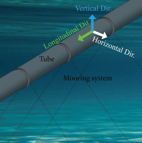
A submerged floating tunnel (SFT) has the potential to drive significant positive changes through shortening sea crossing distances, increasing environmental adaptability, lowering impacts on the local flora and fauna, and reducing construction costs. The SFT segments are moored afloat from the seafloor by means of an underwater mooring system. A typical SFT system is shown in Fig. 1. In the vertical plane, mooring lines or tethers help to provide sufficient vertical stiffness, and additionally, ballast adjustment balances the vertical loads, and controls the buoyancy weight ratio (BWR), which determines the net buoyancy acting on the SFT tube. However, only inclined mooring lines provide horizontal stiffness to the SFT system. Thus, in-line force on the SFT cross section (horizontal load comprises the drag and inertial force) has a major impact on the reliability of the SFT, and an accurate computation of in-line force becomes vital. The in-line force on the SFT tube is mainly determined by cross-sectional geometry and hydrodynamic loading. A parametric Bézier curve defined the SFT cross-sectional geometry in our previous research, showing better hydrodynamic performance than the simpler shapes under uniform current, tsunami, and typhoon conditions (P. Zou et al., 2020; Zou et al., 2020a, 2020b). However, hydrodynamic performance analysis of the SFT under tidal flow conditions, and detailed understanding of the physics of flows around the SFT surface, are still absent. To guarantee safety of ship navigation, the submergence depth of the SFT is typically below 40 m, where the surface wave action on the SFT is effectively reduced (Seo et al., 2015). Therefore, in this study, bidirectional and transient tidal flow is considered the main hydrodynamic forcing, where Reynolds number (R_e) varies greatly, and may induce transition processes in the boundary layer. The laminar–turbulent transition phenomenon prediction is still challenging due to the high complexity of the flow mechanism in the thin boundary layer. The surface roughness of the SFT cross-section and the freestream turbulence intensity should be insufficient to trigger a bypass transition, but the transition modes can be diverse at different R_e. Thus, a reliable transitional flow resolving method for the in-line force prediction of the SFT is required.

Figure 1 Schematic configuration of an SFT system. The “in-line” force discussed in this paper is the “Horizontal Dir.” force shown

Transition phenomena are ubiquitous in the internal and external flows seen in the aerospace industry, turbomachinery applications, and offshore engineering. The transition process can be simply expounded by a laminar boundary layer, the thickness and instabilities of which grow rapidly, forming a transition region of turbulent flow (Durbin, 2017). The transition modes occur though different mechanisms under different conditions, generally referred to as natural, bypass and separation-induced transitions. Natural transition, caused by travelling Tollmien–Schlichting (TS) waves destabilizing the laminar boundary layer, occurs with a low freestream turbulence intensity. The laminar boundary layer becomes unstable beyond a critical R_e, resulting in exponential growth of TS waves, nonlinear breakdown to turbulent spots, and eventually fully-turbulent flow (Edward Mayle, 1991; Schlichting & Gersten, 2016). Bypass transition occurs generally due to high freestream turbulence intensity T_u (> 1%), surface roughness perturbations or injected turbulent flows, which are widely applied in turbine blade research and design (Jacobs & Durbin, 2001; Langtry & Menter, 2009). The separation-induced transition develops when the laminar boundary layer separates under the impact of a strong adverse pressure gradient and may form a shear layer that reattaches. The flow separation occurs due to instabilities that develop, forming periodic roll-up vortices and interacting with the structure surface. The near-wall fluid is then ejected into the freestream, releasing large eddies into the shear layer and generating periodic bubbles. Separation-induced transition can be further classified as a transitional separation mode and laminar separation with short or long bubble modes (Hatman & Wang, 1999).

In recent years, high-precision boundary layer transition prediction methods have been rapidly developed. An empirical transition correlation-based method (Langtry & Menter, 2009) has been developed called the transition SST model ($\stackrel{~}{{\mathsf{R}}_{\mathsf{e}\mathsf{\text{θ}}\mathsf{t}}}$ model), and flat-plate numerical simulations show good agreement with experimental data ranging from bypass transition to natural transition and separation-induced transition. Smith (1956), and Van Ingen (1956) proposed another semi-empirical transition prediction method named the e^N method, which was widely applied combining a potential flow panel method coupled with a boundary layer formulation using the 2D panel code XFoil for airfoil design (Drela, 1989). Walters and Cokljat (2008) developed a k-k_L-ω model based on a three-equation eddy-viscosity formulation, including the k-ω framework and an additional transport equation for the laminar fluctuations of kinetic energy k_L to predict the magnitude of low-frequency velocity fluctuations in the pre-transitional boundary layer; this model also proved to be an effective boundary layer development prediction tool. Low Reynolds number damping functions were first introduced by Wilcox (1994) for the k-ω model to predict viscous sublayer behaviour. Matin Nikoo et al. (2019) applied the low Reynolds number correction technique to a 3D vortex-induced vibration (VIV) simulation of a cylinder and achieved higher accuracy of VIV response estimation than previous studies. Direct numerical simulations (DNS) or large eddy simulations (LES) can provide more accurate transition process prediction (Liu & Chen, 2011; Mary & Sagaut, 2002), but both of the two methods are prohibitive with respect to computational requirements.

This paper aims to better understand the transition phenomenon and predict it accurately for the SFT, and to determine a well-performing SFT cross-section geometry. In Section 2, the methodology of the transition model and the SFT cross-section geometry are illustrated. Validations of various transition models including the e^N method, the low-Reynolds number turbulence model, the k-k_L-ω transition model, and the transition SST model are conducted to determine the most suitable method for the SFT in Section 3. The preferable SFT cross-sectional geometry and aspect ratio (AR) under tidal flow conditions is proposed, and the effect of turbulence parameters on hydrodynamic performance prediction are also discussed in Section 4.

2 CFD methodology

2.1 Parametric Bézier curves

An airfoil geometry parameterization method based on the Bézier-PARSEC (BP) curve (Derksen & Rogalsky, 2010) combining the merits of the Bézier curve with PARSEC variables is employed in the SFT cross-section design. Considering the possibility of bi-directional (i.e. tidal) flow of the SFT, the leading and trailing halves of the SFT cross-section are designed to be symmetric. Furthermore, a cross-section with symmetric upper and lower surfaces can reduce the root mean square lift (F_y,rms) fluctuation and hence simplify buoyancy control of the SFT. Thus, a BP parameterization using a third degree Bezier curve and a quadrant comprising of four control points is applied to define the SFT’s geometry, given by Eq. (1): (1) $\begin{array}{r}\left\{\begin{array}{l}x\left(u\right)=-x_0{u}^3+3x_1(u\text{ + 1)}{u}^2-3x_2(u+1{)}^{2}u+x_3(u+1{)}^3\\ y\left(u\right)=-y_0{u}^3+3y_1(u\text{ + 1)}{u}^2-3y_2(u+1{)}^{2}u+y_3(u+1{)}^3\end{array}\right.\end{array}$(1) where u is a variable with the range of −1 to 0.

Due to the sharp trailing-edge of normal airfoils, the Kutta condition (Crighton, 1985) can be met, which effectively precludes the possibility of vortex shedding, and hence, reduces the in-line force. Therefore, the BP curve composed by the trailing-edge profile is applied to describe the SFT cross-section. However, in order to compare the impacts of different types of Bezier curves and AR (defined by y_t/x_t) on the hydrodynamic response of the SFT, the BP curve composed by the leading-edge profile is also adopted to define the SFT cross-section geometry. The parametric Bézier curve of each quadrant and control points are shown in Fig. 2.

Figure 2 Control points of the third-degree Bézier curves of each quadrant. (a) Leading-edge BP curve; (b) trailing-edge BP curve

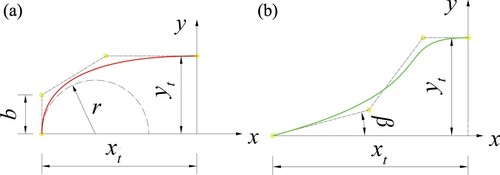
The four control points that determine the shape of one quadrant of the SFT cross-section using trailing-edge and leading-edge BP curves are given by Eqs (2) and (3), respectively: (2) $\begin{array}{rl}& \left\{\begin{array}{l}{x}_0=0,y_0=y_t\\ x_1=-x_t+3b^2/2r\text{, }{y}_1=y_t\\ x_2=-x_t+b\cot \text{β}\text{, }{y}_2=b\\ x_3=-x_t\text{, }{y}_3=0\end{array}\right.\end{array}$(2) (3) $\begin{array}{rl}& \left\{\begin{array}{l}{x}_0=-x_t,y_0=0\\ x_1=-x_t,y_1=b\\ x_2=-x_t+3b^2/2r,y_2=y_t\\ x_3=0,y_3=y_t\end{array}\right.\end{array}$(3) where x_t and y_t are half of the SFT’s width and height, respectively, r is leading-edge radius, and b and β are Bezier curve parameters.

2.2 SFT cross-section

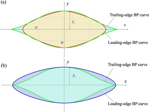
Referring to the current technical standards, and the requirement of carriageway clearance for traffic, space utilization for ventilation ducts, and service utilities including traffic signals, signboards, evacuation passageways, and sidewalks (AASHTO, 2018; ITA Working Group on General Approaches to the Design of Tunnels, 1988), an SFT cross-section with lateral and vertical clearances of W = 11 m and H = 5 m, respectively, is chosen for analysis (Fig. 3a). b = 1.5 m, r = 0.5 m, and β = 15° are selected and y_t values of 3, 4 and 5 m are applied, respectively, in the sensitivity analysis of cross-sectional AR. The SFT cross-sections expressed by the leading-edge and trailing-edge BP curves with the same clearance are shown in Fig. 3a. However, an SFT cross-section of the same clearance defined by different BP curves causes inconsistency in AR. In order to determine the best BP curve type in improving the hydrodynamic performance, but eliminate the impacts of AR, another subset of leading-edge and trailing-edge BP curves under the same AR is chosen for comparison (Fig. 3b).

Figure 3 Leading-edge and trailing-edge BP curve geometry. (a) Equal clearance; (b) equal AR

2.3 Transition modelling

e^N method

The e^N method is based on local linear stability theory and a parallel flow assumption, and calculates local amplification rates of unstable waves by solving the local stability equations or the parabolized stability equations (PSE). The N factor as a function of a given location and frequency can be determined by Eq. (4). Transition is assumed to occur if N reaches a threshold N value obtained from experimental correlations (Van Ingen, 1956): (4) $N=-8.43-2.4\ln \left(T_u\right)$(4)

k-k_L-ω transition model

The k-k_L-ω transition model is used to calculate transition onset and effectively address the transition of the boundary layer from laminar to turbulent. It is a three-equation eddy-viscosity model including laminar fluctuations of kinetic energy k_L, turbulent kinetic energy k_T, and the inverse turbulent time scale ω, given by Eq. (5): (5) $\begin{array}{r}\left\{\begin{array}{l}\frac{\text{D}{k}_T}{\text{D}t}=P_{k_T}+R+R_{NAT}-\omega k_T-D_T\\ \phantom{\frac{\text{D}{k}_T}{\text{D}t}=}+\frac{\mathrm{\partial }}{\mathrm{\partial }{x}_j}\left[\left(\nu +\frac{{\alpha }_T}{{\alpha }_k}\right)\frac{\mathrm{\partial }{k}_T}{\mathrm{\partial }{x}_j}\right]\\ \frac{\text{D}{k}_L}{\text{D}t}=P_{k_L}-R-R_{NAT}-D_T+\frac{\mathrm{\partial }}{\mathrm{\partial }{x}_j}\left[\nu \frac{\mathrm{\partial }{k}_L}{\mathrm{\partial }{x}_j}\right]\\ \frac{\text{D}\omega }{\text{D}t}=C_{\omega 1}\frac{\omega }{k_T}{P}_{k_T}+\left(\frac{C_{\omega R}}{f_W}-1\right)\frac{\omega }{k_T}(R+R_{NAT})-C_{\omega 2}{\omega }^2\\ \phantom{\frac{\text{D}\omega }{\text{D}t}=}-C_{\omega 3}{f}_{\omega }{\alpha }_T{f}_W^2\frac{\sqrt{k_T}}{d^3}+\frac{\mathrm{\partial }}{\mathrm{\partial }{x}_j}\left[(\nu +\frac{{\alpha }_T}{{\alpha }_{\omega }})\frac{\mathrm{\partial }\omega }{\mathrm{\partial }{x}_j}\right]\end{array}\right.\end{array}$(5) where P_kT is the turbulence production term; k_T is large scale energy; α_T is turbulent scalar diffusivity; D_T is near-wall dissipation; R_NAT is the natural transition production term; C_ω1 = 0.44; C_ω2 = 0.92; C_ω3 = 0.3; C_ωR = 1.5. For details see Walters and Cokljat (2008).

Low-Reynolds number model

Low-Reynolds number correction (Fluent, 2013) can also be used to predict transition, and is compatible with modern CFD codes without any coupling to empirical correlations. A coefficient α* implemented in the k-ω model damps the turbulent viscosity, given by Eqs (6–8): (6) $\begin{array}{rl}{\alpha }^{\ast }& ={\alpha }_{\mathrm{\infty }}^{\ast }\left(\frac{{\alpha }_0^{\ast }+{{\mathsf{R}}_{\mathsf{e}}}_{\mathsf{t}}/R_k}{1+{{\mathsf{R}}_{\mathsf{e}}}_{\mathsf{t}}/R_k}\right)\end{array}$(6) (7) $\begin{array}{rl}{\mathsf{R}}_{{\mathsf{e}}_{\mathsf{t}}}& =\frac{\rho k}{\mu \omega }\end{array}$(7) (8) $\begin{array}{rl}{R}_k& =6;{\alpha }_0^{\ast }=\frac{{\text{β}}_i}{3};{\text{β}}_i=0.072\end{array}$(8)

Transition SST model

The transition SST model is based on the coupling of the k-ω SST transport equations with the intermittency and momentum-thickness Reynolds number transport equations for the transition onset criteria (Fluent, 2013; Langtry & Menter, 2009). Besides the two-equation model including the k and ω equations of the k-ω SST turbulence model, the additional transport equations of the transition SST model are shown in Eq. (9): (9) $\begin{array}{r}\left\{\begin{array}{l}\frac{\mathrm{\partial }}{\mathrm{\partial }t}\left(\rho \gamma \right)+\frac{\mathrm{\partial }}{\mathrm{\partial }{x}_j}\left(\rho \gamma U_j\right)=\frac{\mathrm{\partial }}{\mathrm{\partial }{x}_j}\left[(\mu +\frac{{\mu }_t}{{\sigma }_{\gamma }})\frac{\mathrm{\partial }\gamma }{\mathrm{\partial }{x}_j}\right]+P_{\gamma 1}-E_{\gamma 1}\\ \phantom{\frac{\mathrm{\partial }}{\mathrm{\partial }t}\left(\rho \gamma \right)+\frac{\mathrm{\partial }}{\mathrm{\partial }{x}_j}\left(\rho \gamma U_j\right)=}+P_{\gamma 2}-E_{\gamma 2}\\ \frac{\mathrm{\partial }}{\mathrm{\partial }t}\left(\rho \stackrel{~}{{\mathsf{R}}_{\mathsf{e}\mathsf{\text{θ}}\mathsf{t}}}\right)+\frac{\mathrm{\partial }}{\mathrm{\partial }{x}_j}\left(\rho \stackrel{~}{{\mathsf{R}}_{\mathsf{e}\mathsf{\text{θ}}\mathsf{t}}}{U}_j\right)=\frac{\mathrm{\partial }}{\mathrm{\partial }{x}_j}\left[{\sigma }_{\theta t}(\mu +{\mu }_t)\frac{\mathrm{\partial }\stackrel{~}{{\mathsf{R}}_{\mathsf{e}\mathsf{\text{θ}}\mathsf{t}}}}{\mathrm{\partial }{x}_j}\right]\\ \phantom{\frac{\mathrm{\partial }}{\mathrm{\partial }t}\left(\rho \widetilde{{\mathsf{R}}_{\mathsf{e}\theta \mathsf{t}}}\right)+\frac{\mathrm{\partial }}{\mathrm{\partial }{x}_j}\left(\rho \widetilde{{\mathsf{R}}_{\mathsf{e}\theta \mathsf{t}}}{U}_j\right)=}+P_{\theta t}\end{array}\right.\end{array}$(9) where σ_γ= 1.0, and σ_θt= 2.0; µ is viscosity; µ_t is eddy viscosity; p_∞ is reference pressure; P_γ1 and E_γ1 are transition sources; P_γ2 and E_γ2 are destruction and relaminarization sources; P_θt is production source term; γ is intermittency; $\stackrel{~}{{\mathsf{R}}_{\mathsf{e}\mathsf{\text{θ}}\mathsf{t}}}$ is transition momentum thickness Reynolds number; ρ is fluid density; and U is upstream flow velocity. Detailed derivation of transition, production, destruction and relaminarization sources, and the transition onset controlling algorithm are given in Fluent (2013).

The decay of the turbulent kinetic energy can be rewritten in terms of inlet T_uinlet and eddy viscosity ratio µ_t/µ as Eq. (10): (10) $T_u={\left\{T_{u_{inlet}}^2{\left[1+\frac{3\rho Vx\text{β}\left(T_{u_{inlet}}^2\right)}{2\mu {\left({\mu }_t/\mu \right)}_{inlet}}\right]}^{-\text{β}\ast /\text{β}}\right\}}^{0.5}$(10) where β = 0.09, and β* = 0.0828; V is mean convective velocity; and x is streamwise distance downstream of the inlet.

T_uinlet can be estimated in terms of turbulent kinetic energy k and turbulent dissipation rate $ϵ$, as shown in Eqs (11) and (12). (11) $\begin{array}{rl}k& =\frac{3}{2}(U\cdot T_u{)}^2\end{array}$(11) (12) $\begin{array}{rl}ϵ& =\frac{k^{3/2}}{l}\end{array}$(12) where ε is turbulence dissipation rate; l is turbulence length scale and can be computed by the boundary layer thickness δ₉₉, shown as Eq. (13): (13) $l=0.4{\delta }_{99}$(13)

3 Modelling validation

3.1 Low ${\mathsf{R}}_{\mathsf{e}}$ validation

The Eppler airfoil is used to validate the two-dimensional (2D) transition models at low R_e using the CFD code ANSYS FLUENT v19.1. Transition turbulence models include the k-k_L-ω model, the k-ω SST-LR model (standard SST k-ω model with a low-Reynolds number correction), and the transition SST model are validated against the Langley low-turbulence wind-tunnel experiments (McGhee et al., 1988). The transition prediction of the airfoil using the e^N method is also compared. The first grid layer length normal to the airfoil surface meets the requirement of y⁺ < 1. T_uinlet = 0.07% and hydraulic diameter = 1.524 m are adopted at the inlet boundary of the CFD simulations. For the e^N method, the airfoil is defined with 250 points, and the threshold N value of 9 is set, corresponding to a smooth wing surface in a low turbulence intensity freestream.

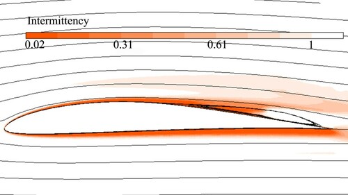
Figure 4 compares simulation results with experimental data for the time-averaged pressure coefficient C_p,m distribution (defined by C_p= (p – p_ref)/(0.5U²), where p is the pressure on the structure; p_ref is the reference pressure) in the range x/c = 0–1 (c is the chord length for an airfoil, and the cross-sectional width for an SFT) at different R_e. It can be seen that by using the transition SST model and e^N method, the transition scenarios, plateau and suction peak values are well predicted compared with the experiment data, although a considerable discrepancy and slight underestimation of upper surface pressure is observed. Additionally, the plateau after the suction peak value and the sharp increase after the plateau upstream of the trailing edge underlines the existence of flow separation, and both the laminar separation (LS) and turbulent reattachment (TR) points can be satisfactorily detected and are consistent with the experimental data and the oil flow visualization of the experiment test (McGhee et al., 1988). However, neither the k-k_L-ω turbulence model nor the k-ω SST-LR model is satisfactory for pressure estimation, and the transition and separation processes cannot be clearly predicted. As exhibited by Fig. 4a, a local region of laminar separated flow near the leading edge, reattaches to the downstream surface, generating separation bubbles (SB). At R_e = 6 × 10⁴, the transition onset is induced downstream of the LS point by inflexional instability and ejection processes, implying the transition of laminar separation with long bubble mode generation (Fig. 5).

Figure 4 Predicted and measured time-averaged pressure distribution using different methods. (a) R_e = 4.6 × 10⁵; (b) R_e = 6 × 10⁴. Abbreviations: LS, laminar separation; TR, turbulent reattachment; SB, separation bubble

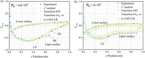
Figure 5 Intermittency contours and streamlines around the airfoil at R_e = 6 × 10⁴

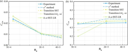
Figure 6a shows that the time-averaged drag coefficient (C_d,m) decreases with increasing R_e (drag coefficient C_d is defined as C_d = F_x/(0.5 × ρ × U²× c), where F_x is the horizontal force). In comparison to the experimental data at R_e = 6 × 10⁴, the time-averaged pressures near the trailing edge of the lower surface computed by the k-k_L-ω and k-ω SST-LR models do not exceed p_∞ (Fig. 4b), hence overestimating the drag. At R_e = 4.6 × 10⁵, the k-ω SST-LR model overestimates the drag due to its limitations in adequately predicting realistic boundary layer behaviour, the transition process and flow separation at high R_e. Figure 6b provides a comparison of the time-averaged lift coefficient (C_l,m) of the numerical results with the experimental data (C_l is the lift coefficient defined by C_l = F_y/(0.5 × ρ × U²× c), where F_y is the vertical force). The e^N method underpredicts the values of C_pb compared with the other turbulence models and measured data (Fig. 4), resulting in a noticeable overestimation of lift at R_e = 2 × 10⁵ and 4.5 × 10⁵. Moreover, the k-k_L-ω and k-ω SST-LR models show a clear deviation of C_l at R_e = 6 × 10⁴ due to the poorly predicted pressure aforementioned. Comparison with other numerical tools confirms that the transition SST model is an adaptable and reliable method to predict the transition process at low Reynolds numbers, and to compute drag and lift.

Figure 6 Predicted and measured time-averaged hydrodynamic properties using different methods. (a) C_d,m; (b) C_l,m

The transition SST model introduces an effective intermittency to modify the production and destruction terms in turbulent kinetic energy equation. Moreover, the supplementary transport equation for $\stackrel{~}{{\mathsf{R}}_{\mathsf{e}}{{}_{\text{θ}}}_{\mathsf{t}}}$ assures capture of the strong variation of the turbulence intensity, improving the transition prediction. However, note that the transition SST model is not proposed to simulate the physics of the transition process but is essentially an experimental correlation-based model. It was found to be strongly dependent on the selected correlation for the critical Reynolds number (Richez et al., 2016), with limitations in predicting massive separation flows (Shi & Wang, 2021).

3.2 High ${\mathsf{R}}_{\mathsf{e}}$ validation

To verify the reliability of the transition SST model at high R_e, the natural laminar airfoil NLF(1)-0416 is selected. Simulation results from a 2D model are compared with experimental data by Somers (1992) from a low-turbulence wind tunnel.

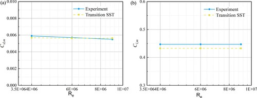
At high R_e of 4 × 10⁶, the first grid layer length normal to the airfoil surface meets the requirement of y⁺ < 1. T_uinlet = 0.07%, hydraulic diameter = 1.524 m, and γ = 1 are adopted in the inlet boundary. Figure 7 shows $C_{p,m}$ and $C_{f,m}$ distributions (skin-friction coefficient C_f is defined by C_f= τ_ω/(0.5 × ρ × U²), where τ_ω is local wall shear stress) from the transition SST model and the experiment. Figure 7a indicates that the pressure and suction sides captured by the transition SST model are in close agreement with the experiment, despite a slight overestimation on the upper surface. The transition effect in the boundary layer and onset locations can be accurately predicted by the transition SST. The sudden increase of the pressure and dramatic increase in skin friction resemble laminar separation with short bubble transition mode, characterized by a quick transition completion due to a complex interaction between the separated shear layer and the reverse flow vortex (Hatman & Wang, 1999), which can be clearly seen at around 40% and 60% chord on the upper and lower surfaces, respectively. It can also be verified by Fig. 8 where the intermittency change from 0 to 1 indicates the onset of the transition point. Figure 9 shows C_d,m and C_l.m predictions under various high R_e, indicating that the transition SST model is capable of accurately predicting the hydrodynamics of the SFT with a maximum deviation of 3% compared with the experiment data.

Figure 7 Predicted and measured time-averaged hydrodynamic properties at R_e = 4 × 10⁶. (a) C_p,m; (b) $C_{f,m}$

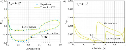
Figure 8 Intermittency contours at R_e = 4 × 10⁶

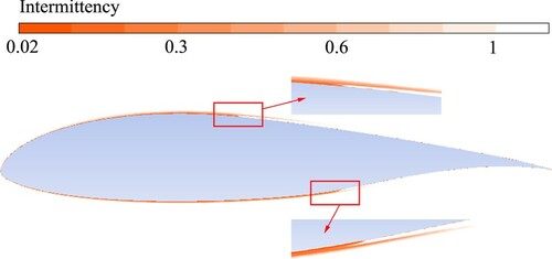
Figure 9 Predicted and measured time-averaged hydrodynamic properties at R_e = 4 × 10⁶. (a) C_d,m; (b) C_l,m

4 Results and discussion

4.1 Grid independent limit test

A grid independent limit (GIL) test for different grid refinement levels is carried out in order to ensure the independence of the hydrodynamic performance of the SFT to the adopted mesh size. 2D CFD models with various grid configurations were established (Fig. 10). The computational domain is 20 W in length and 5 W in height. A zero-reference pressure and zero-gradient condition for velocity are employed at the pressure-outlet boundary. A simplified no-slip hydraulically smooth wall condition is applied on the SFT cross-section surface. Symmetry (free-slip) is used to avoid wall effects at both the upper and lower boundaries. The distances from the inlet and outlet boundaries to the SFT cross-section centre are 5 W and 15 W, respectively. A high-quality unstructured mesh is generated around the SFT cross-section surface, and an inflation tool is used to generate 40 layers of quadrangular cells covering the boundary layer. The first grid layer cell length normal to the SFT surface is 3 × 10⁻⁵ m with a growth rate of 1.2, such that the wall y⁺ is around 1. The computational mesh is divided into three domains with different cell sizes. The first cell size (S₁) is the cell size parallel to the SFT cross-section surface. The second cell size (S₂) is the maximum unstructured mesh size around the SFT. The third cell size (S₃) is the maximum structured mesh size in the rest of the domain. The three cell sizes and the calculated mean in-line force (F_x,m) and the root mean square of cross-flow force (F_y,_rms) are tabulated in Table 1. This shows that Case 2 has almost identical simulation results as Case 3 (hence is regarded as converged) but fewer total cells, which saves computational cost. Thus, Case 2 is chosen for all analysed cases, with a minimum orthogonality of 0.46 after mesh improvement. The maximum CFL number was 0.5, and the non-dimensional time step δtU/W was kept below 5 × 10⁻⁴. The PISO (pressure-implicit with splitting of operators) algorithm is used for pressure–velocity coupling. A high-performance computing (HPC) cluster is used to run parallel computation tasks.

Figure 10 Mesh grids schematic. (a) The distribution of computational mesh; (b) detailed mesh near the SFT cross-section surface

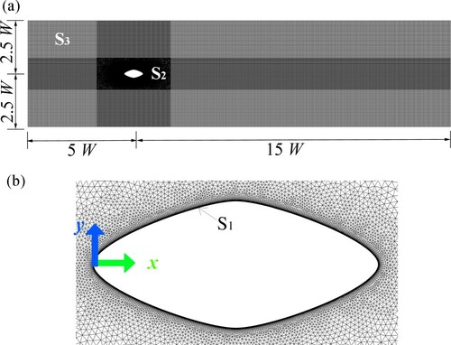
Table 1 Mesh size for the GIL test

	S1 (m)	S2 (m)	S3 (m)	NCells	Fx,m (N)	Fy,rms (N)
Case 1	0.02	0.5	1	258,530	151.45	153.16
Case 2	0.01	0.5	1	356,792	149.54	114.33
Case 3	0.01	0.25	0.5	585,404	150.36	114.07

4.2 Effect of freestream turbulence parameters

Transition prediction is affected by factors such as surface roughness, surface geometry, turbulence intensity, pressure distribution and fluid property, Mach number and Reynolds number. Several methods can be applied to specify the inlet turbulence parameters in ANSYS Fluent; freestream quantities of turbulence intensity T_u and turbulence length scale l are specified at the inlet boundary.

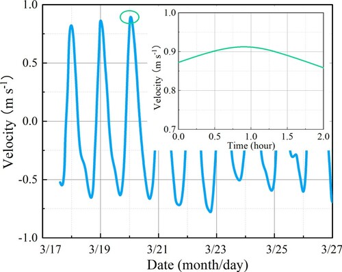
The Qiongzhou strait, located between Hainan island and the Leizhou Peninsula in southern China, is regarded as a potential SFT application site (Jiang et al., 2018; Yan et al., 2016). For the flow conditions in the Qiongzhou Strait (simplified as a wide open channel), the boundary layer thickness is assumed to be the entire channel depth (Kironoto & Graf, 1995). Zhu et al. (2015) carried out a 15-day coastal acoustic tomography experiment to quantity the tidal current in the Qiongzhou Strait over a fortnightly spring-neap tidal cycle. A representative time series of the section-averaged velocity (station pairs C3–C4 in Zhu et al., 2015) is adopted as the CFD inlet boundary condition (Fig. 11). As per the previous research (Zou et al., 2020b), due to the slow variation of the tidal current speed, it was proved that drag has a larger effect than inertial force. To reduce computational cost, we take a 2-h window around peak velocity (the green circle in Fig. 11) from an entire 24 h transient tidal cycle as the inlet velocity boundary for all the transient simulations. Considering the submergence depth of the SFT, $ϵ=9.5\times {10}^{-9}\text{W}\text{k}{\text{g}}^{-\text{1}}$ measured at a depth of 34–36 m near the Qiongzhou Strait (Li et al., 2018) is applied, and hence, the freestream turbulence intensity T_uinlet and l can be derived using Eqs (11–13) and obtained as 0.006 U^–1 (over 0.6%) and 40 m, respectively.

Figure 11 Measured tidal velocities in the Qiongzhou Strait

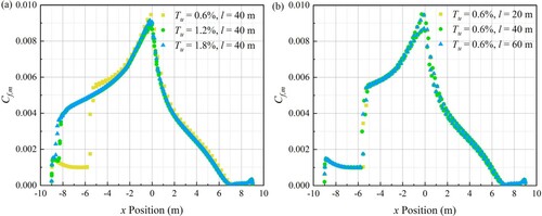
In order to investigate the effect of freestream turbulence parameters on the hydrodynamic performance of the SFT, $C_{f,m}$ distributions under different T_uinlet and l combinations are plotted in Fig. 12. This shows that with increasing T_uinlet, the transition onset location moves noticeably forward, and the transition process is imposed and finished instantaneously far upstream when T_uinlet > 1.2%, and in this case, a fully-turbulent model can be supposed as an alternative. However, no obvious impact of l is found on $C_{f,m}$ distributions. We conclude that T_u is a crucial factor, and contributes to determining the transition location and the accuracy of the transition process prediction.

Figure 12 Sensitivity analysis of the freestream turbulence parameters. (a) Turbulence intensity; (b) turbulence length scale

Langtry et al. (2006) found that the three-dimensional model is essential when there is a significant amount of separated flow under a high angle of attack, particularly near stall conditions. However, our simulations show no flow separation in the transition region of the SFT, indicating the applied two-dimensional modelling is sufficient in transition prediction accuracy and practical in reducing computational loads.

4.3 Comparison with the fully-turbulent model

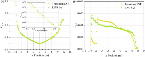
The R_e of an SFT subject to tidal flow varies greatly, with a maximum magnitude in the order of 10⁷. To further examine the difference between the transition turbulence model and the widely used fully-turbulent model on hydrodynamic performance prediction, the RNG k-ε turbulence model is used for comparison. The first grid layer cell length normal to the cross-section surface is 0.004 m with the standard wall function in the RNG k-ε turbulence model, restricting y⁺ to 30–200, while other grid sizes (the controlling cell size: S₁, S₂ and S₃) keep the same mesh configuration as the transition SST model. A leading-edge BP curve with y_t = 3 m, T_uinlet = 0.6%, and l = 40 m is specified for the two models.

The $C_{p,m}$ and $C_{f,m}$ distributions of the SFT using transition SST and RNG k-ε models are plotted in Fig. 13. The overall pressure distribution is similar for both cases, but with a slight difference in the wake region. However, a small mismatch is observed by further inspection at around x = −9 to −8.5 m. The small step in the transition SST model result indicates the transition process, which cannot be captured by the fully-turbulent model. A low level of skin friction between x = −12 m and x = −9 m is observed in the transition SST model (Fig. 13b), indicating a laminar boundary layer followed by precipitous triggering of an enhancement and the formation of the natural transition process. $C_{f,m}$ undergoes a sharp increase at around x = −9 m. This represents the onset of the transition process, and shows inconsistency with Fig. 13a. Furthermore, an obvious difference can be observed between the two models after the transition process due to the differing prediction of transition and boundary layer convection. However, the RNG k-ε turbulence model results yield close agreement with the transition SST model predictions when the flow turns fully-turbulent farther downstream. Both models have the ability to resolve fully-turbulent flows. However, the transition SST model is more reliable over a wider range of applications and confidently reproduces complex flow features, especially at low freestream turbulence intensity conditions.

Figure 13 Comparison between transition SST and RNG k-ε models. (a) $C_{p,m}$; (b) $C_{f,m}$

4.4 Cross-sectional geometry performance comparison

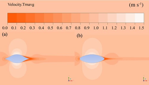
In order to determine the best cross section shape for the hydrodynamic performance of the SFT, $C_{f,m}$ distributions over the SFT cross-section expressed by leading-edge and trailing-edge BP curves under constant AR with varying y_t are illustrated in Fig. 14. It can be seen that the peak $C_{f,m}$ increases with increasing y_t for both BP curve formats. $C_{f,m}$ close to zero corresponds to flow separation and the subsequent wake extension. A narrow flow separation at the rear can be observed at y_t = 3 m using the leading-edge BP curve. However, no flow separation occurs with the trailing-edge BP curve, where the Kutta condition can be met (Crighton, 1985). The flow separation point moves noticeably forward with increasing y_t. Compared with the leading-edge BP curve, as y_t increases, a further forward separation point and larger wake region can be seen from the trailing-edge BP curve. This can be seen in Fig. 15, which shows time-averaged velocity contours of the two curve formats at y_t = 4 m. As y_t increases, the apex of the trailing-edge BP curve is sharper and less streamlined. The bluffer shape results in the streamflow passing the apex, detaching from the surface, and forming a large wake of recirculating flow, which also increases the in-line force.

Figure 14 Time-averaged skin-friction coefficient distribution. (a) y_t = 3 m; (b) y_t = 4 m; (c) y_t = 5 m

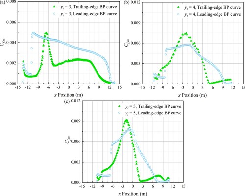
Figure 15 Time-averaged velocity contours at y_t = 4 m. (a) Trailing-edge BP curve; (b) leading-edge BP curve

4.5 Cross-sectional aspect ratio performance comparison

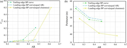
Figure 16 shows the mean drag coefficient C_d,m and perimeter of the different SFT cross-sectional geometries and aspect ratios. It can be seen clearly that as AR increases, C_d,m on the trailing-edge BP curve increases rapidly compared with the leading-edge one (equal AR), indicating the leading-edge format has a better hydrodynamic performance. However, continuously increasing AR makes the geometry bluffer, and C_d,m increases dramatically when AR > 0.47. In this case, an AR not exceeding 0.47 using a leading-edge BP curve is preferred. In addition to hydrodynamic performance, the SFT cross-section design is affected by clearance requirements, structural safety, and construction costs. It can be found from Fig. 16a that C_d,m on the two formats of leading-edge BP curves (equal AR and equal clearance) are similar in general. However, the SFT cross-sectional perimeter can be effectively shortened with a leading-edge BP curve of equal clearance (Fig. 16b). Therefore, the SFT cross-section with AR = 0.47 using a leading-edge BP curve of equal clearance balances hydrodynamic forcing and material costs well.

Figure 16 Drag coefficient and perimeter of the SFT cross-section. (a) Mean drag coefficient comparison; (b) perimeter comparison

5 Conclusion

In order to determine a reasonable aspect ratio and geometry of the SFT cross-section, two formats of parametric Bézier curves are tested. Various turbulence models for SFT hydrodynamic performance prediction are compared under bidirectional and unsteady current conditions to determine the most appropriate transition prediction method for the SFT’s in-line force computation. The effect of inflow turbulence parameters (turbulence intensity and turbulence length scale) on the transition location is discussed in detail. A reasonable aspect ratio and geometry of the SFT cross-section has been presented for practical engineering application. The main conclusions are briefly summarized as follows:

1. Analysing the differences between experimental measurements and results computed with turbulence models based on the e^N method, the low-Reynolds number turbulence model, the k-k_L-ω transition model, and the transition SST model, the transition SST model shows the capability to accurately compute the hydrodynamic performance at both low and high Reynolds numbers.

2. Compared with the transition SST turbulence model, a separation-capturing and laminar-turbulent transition process cannot be achieved by a fully-turbulent simulation, especially at low freestream turbulence intensity conditions, affecting the accuracy of the SFT hydrodynamic performance prediction.

3. The freestream turbulence intensity has an influence on the transition location, affecting the accuracy of the transition process simulation and hydrodynamic performance prediction. However, the effect of turbulence length scale is relatively minor.

4. By increasing the aspect ratio, the SFT cross-section described by the leading-edge BP curve shows better hydrodynamic performance than the trailing-edge BP curve. Additionally, the SFT cross-section with AR = 0.47 using the leading-edge BP curve under the given clearance appears the best option with a balanced consideration of hydrodynamic performances and construction cost.

Notation

b	=	Bezier curve parameter (m)
c	=	chord length (m)
Cd,m	=	time-averaged drag coefficient (–)
$C_{f,m}$	=	time-averaged skin-friction coefficient (–)
Cl,m	=	time-averaged lift coefficient (–)
$C_{p,m}$	=	time-averaged pressure coefficient (–)
DT	=	near-wall dissipation (m2 s−3)
Eγ1	=	transition source (m2 s−3)
Eγ2	=	relaminarization source (m2 s−3)
Fx	=	horizontal force (N)
Fy	=	vertical force (N)
H	=	cross-sectional vertical clearance (m)
k	=	turbulent kinetic energy per unit mass (m2 s−2)
kT	=	large scale energy (m2 s−2)
l	=	turbulence length scale (m)
p∞	=	reference pressure (Pa)
PkT	=	turbulence production term (m2 s−3)
Pγ1	=	transition source (m2 s−3)
Pγ2	=	destruction source (m2 s−3)
Pθt	=	production source term (m2 s−3)
r	=	leading-edge radius (m)
Re	=	Reynolds number (–)
$\stackrel{~}{{\mathsf{R}}_{\mathsf{e}}{{}_{\text{θ}}}_{\mathsf{t}}}$	=	transition momentum thickness Reynolds number (–)
RNAT	=	natural transition production term (m2 s−3)
t	=	time (s)
Tu	=	turbulence intensity (%)
Tuinlet	=	inlet turbulence intensity (%)
U	=	upstream flow velocity (m s−1)
V	=	mean convective velocity (m s−1)
W	=	cross-sectional lateral clearance (m)
x	=	streamwise distance downstream of the inlet (m)
xt	=	half of the cross-sectional width (m)
yt	=	half of the cross-sectional height (m)
αT	=	turbulent scalar diffusivity (m2 s−1)
β	=	Bezier curve parameter (m)
γ	=	intermittency (–)
δ99	=	boundary layer thickness (m)
ε	=	turbulent dissipation rate (m2 s−3)
μ	=	fluid viscosity (Pa s)
μt	=	eddy viscosity (Pa s)
ρ	=	fluid density (kg m−3)
τω	=	local wall shear stress (N m−2)

Acknowledgements

The study presented in this paper was conducted in the submerged floating tunnel research project funded by China Communications Construction Company Ltd. (CCCC). The authors would like to acknowledge C.J. (Carlos) Simão Ferreira for his contribution in elucidating the knowledge of airfoil design and giving his comments to this study.

References

- American Association of State Highway and Transportation Officials (AASHTO). (2018). Policy on geometric design of highways and streets (7th Edition) (pp. 4-60–4-63). American Association of State Highway and Transportation Officials (AASHTO). Retrieved from https://app.knovel.com/hotlink/toc/id:kpPGDHSE12/policy-geometric-design/policy-geometric-design
- Crighton, D. G. (1985). The Kutta condition in unsteady flow. Annual Review of Fluid Mechanics, 17(1), 411–445. https://doi.org/https://doi.org/10.1146/annurev.fl.17.010185.002211
- Derksen, R. W., & Rogalsky, T. (2010). Bezier-PARSEC: An optimized aerofoil parameterization for design. Advances in Engineering Software, 41(7-8), 923–930. https://doi.org/https://doi.org/10.1016/j.advengsoft.2010.05.002
- Drela, M. (1989). XFOIL: an analysis and design system for low Reynolds number airfoils. In LOW REYNOLDS NUMBER AERODYNAMICS. PROC. CONF., NOTRE DAME, U.S.A., JUNE 5-7, 1989 }EDITED BY T.J. MUELLER]. (LECTURE NOTES IN 54, 1–12. https://doi.org/https://doi.org/10.1007/978-3-642-84010-4_1
- Durbin, P. A. (2017). Perspectives on the phenomenology and modeling of boundary layer transition. Flow, Turbulence and Combustion, 99(1), 1–23. https://doi.org/https://doi.org/10.1007/s10494-017-9819-9
- Edward Mayle, R. (1991). The 1991 IGTI scholar lecture: the role of laminar-turbulent transition in gas turbine engines. Journal of Turbomachinery, 113, 509–536. https://doi.org/https://doi.org/10.1115/1.2929110
- Fluent, A. (2013). Ansys fluent theory guide. ANSYS Inc., USA.
- Hatman, A., & Wang, T. (1999). A prediction model for separated-flow transition. Journal of Turbomachinery, 121, 594–602. https://doi.org/https://doi.org/10.1115/1.2841357
- ITA Working Group on General Approaches to the Design of Tunnels. (1988). Guidelines for the design of tunnels☆. Tunnelling and Underground Space Technology, 3, 237–249. https://doi.org/https://doi.org/10.1016/0886-7798(88)90050-8
- Jacobs, R. G., & Durbin, P. A. (2001). Simulations of bypass transition. Journal of Fluid Mechanics, 428, 185–212. https://doi.org/https://doi.org/10.1017/S0022112000002469
- Jiang, B., Liang, B., Faggiano, B., Iovane, G., & Mazzolani, F. M. (2018). Feasibility study on a submerged floating tunnel for the Qiongzhou strait in China. Maintenance, safety, risk, management and life-cycle performance of bridges – Proceedings of the 9th International Conference on Bridge Maintenance, Safety and Management, IABMAS 2018.
- Kironoto, B. A., & Graf, W. H. (1995). Turbulence characteristics in rough non-uniform open-channel flow. Proceedings of the Institution of Civil Engineers: Water, Maritime and Energy, 112, 336–348. https://doi.org/https://doi.org/10.1680/iwtme.1995.28114
- Langtry, R. B., Gola, J., & Menter, F. R. (2006). Predicting 2D airfoil and 3D wind turbine rotor performance using a transition model for general CFD codes. Collection of technical papers – 44th AIAA Aerospace Sciences Meeting. https://doi.org/https://doi.org/10.2514/6.2006-395
- Langtry, R. B., & Menter, F. R. (2009). Correlation-based transition modeling for unstructured parallelized computational fluid dynamics codes. AIAA Journal, 47, 2894–2906. https://doi.org/https://doi.org/10.2514/1.42362
- Li, M., Xie, L., Zong, X., Zhang, S., Zhou, L., & Li, J. (2018). The cruise observation of turbulent mixing in the upwelling region east of Hainan Island in the summer of 2012. Acta Oceanologica Sinica, 37(9), 1–12. https://doi.org/https://doi.org/10.1007/s13131-018-1260-y
- Liu, C., & Chen, L. (2011). Parallel DNS for vortex structure of late stages of flow transition. Computers and Fluids, 45, 129–137. https://doi.org/https://doi.org/10.1016/j.compfluid.2010.11.006
- Mary, I., & Sagaut, P. (2002). Large eddy simulation of flow around an airfoil near stall. AIAA Journal, 40, 1139–1145. https://doi.org/https://doi.org/10.2514/3.15174
- Matin Nikoo, H., Bi, K., & Hao, H. (2019). Three-dimensional vortex-induced vibration of a circular cylinder at subcritical Reynolds numbers with low-Re correction. Marine Structures, 66, 288–306. https://doi.org/https://doi.org/10.1016/j.marstruc.2019.05.004
- McGhee, R. J., Walker, B. S., & Millard, B. F. (1988). Experimental results for the Eppler 387 airfoil at low Reynolds numbers in the Langley low-turbulence pressure tunnel (Vol. 4062). National Aeronautics and Space Administration, Scientific and Technical Information Division.
- Richez, F., Leguille, M., & Marquet, O. (2016). Selective frequency damping method for steady RANS solutions of turbulent separated flows around an airfoil at stall. Computers and Fluids, 132, 51–61. https://doi.org/https://doi.org/10.1016/j.compfluid.2016.03.027
- Schlichting, H., & Gersten, K. (2016). Boundary-layer theory. Boundary-Layer Theory. https://doi.org/https://doi.org/10.1007/978-3-662-52919-5
- Seo, S.-i., Mun, H.-s., Lee, J.-h., & Kim, J.-h. (2015). Simplified analysis for estimation of the behavior of a submerged floating tunnel in waves and experimental verification. Marine Structures, 44, 142–158. https://doi.org/https://doi.org/10.1016/j.marstruc.2015.09.002
- Shi, L., & Wang, Y. (2021). Numerical investigations on transitional flows around forward and reversed hydrofoils. European Journal of Mechanics – B/Fluids, 85, 24–45. https://doi.org/https://doi.org/10.1016/j.euromechflu.2020.08.008
- Smith, A. M. O. (1956). Transition, pressure gradient, and stability theory. Proceedings IX International Congress of Applied Mechanics.
- Somers, D. M. (1992). Subsonic natural-laminar-flow airfoils. In R. W. Barnwell & M. Y. Hussaini (Eds.), Natural laminar flow and laminar flow control (pp. 143–176). Springer Verlag.
- Van Ingen, J. L. (1956). A suggested semi-empirical method for the calculation of the boundary layer transition region. Technische Hogeschool Delft, Vliegtuigbouwkunde, Rapport VTH-74.
- Walters, D. K., & Cokljat, D. (2008). A three-equation eddy-viscosity model for reynolds-averaged navier-stokes simulations of transitional flow. Journal of Fluids Engineering. https://doi.org/https://doi.org/10.1115/1.2979230
- Wilcox, D. C. (1994). Simulation of transition with a two-equation turbulence model. AIAA Journal, 32, 247–255. https://doi.org/https://doi.org/10.2514/3.59994
- Yan, H., Zhang, F., & Yu, J. (2016). The Lectotype optimization study on submerged floating tunnel based Delphi method. Procedia Engineering, 166, 118–126. https://doi.org/https://doi.org/10.1016/j.proeng.2016.11.574
- Zhu, X. H., Zhu, Z. N., Guo, X., Ma, Y. L., Fan, X., Dong, M., & Zhang, C. (2015). Measurement of tidal and residual currents and volume transport through the Qiongzhou Strait using coastal acoustic tomography. Continental Shelf Research, 108, 65–75. https://doi.org/https://doi.org/10.1016/j.csr.2015.08.016
- Zou, P., Bricker, J., & Uijttewaal, W. (2020). Optimization of submerged floating tunnel cross section based on parametric Bézier curves and hybrid backpropagation - genetic algorithm. Marine Structures, 74, 102807. https://doi.org/https://doi.org/10.1016/j.marstruc.2020.102807
- Zou, P. X., Bricker, J. D., & Uijttewaal, W. (2020a). A parametric method for submerged floating tunnel cross-section design. Proceedings of the International Offshore and Polar Engineering Conference.
- Zou, P. X., Bricker, J. D., & Uijttewaal, W. S. J. (2020b). Impacts of extreme events on hydrodynamic characteristics of a submerged floating tunnel. Ocean Engineering, 218, 108221. https://doi.org/https://doi.org/10.1016/j.oceaneng.2020.108221