Identification of 1-D cavitation model parameters by means of computational fluid dynamics

Abstract

Hydropower is a key energy conversion technology for stabilizing electrical power. When running at full load, a 3-D cavitation vortex rope develops in Francis turbines that acts as an internal source of energy and instability. 1-D models allow this phenomenon to be predicted and the range of safe operating points to be defined. These models involve three parameters: the mass flow gain factor, the wave speed and the second viscosity that must be calibrated. For the first time, the present work aims at identifying these parameters using 3-D URANS cavitating simulations. Two cavitation test cases are considered: a 2-D Venturi and a reduced scale model of a Francis turbine at full load operating conditions. RANS simulations allow the mass flow gain factor to be determined, whereas URANS simulations coupled with an optimization process allow the determination of the wave speed and the second viscosity. The new methodology shows its ability to identify the three parameters.

Keywords:

• Cavitation
• CFD
• RANS
• swirling flows
• turbine
• Venturi
• 1-D model

1 Introduction

Due to the extensive development of new renewable energy sources during the last decades, the electrical power system experiences large load flow fluctuations, since these energy sources are strongly dependent on the meteorological conditions. To manage these fluctuations, other sources of energy are used to help stabilize the electrical grid. Among them, hydraulic power plants, producing clean electricity, are used due to their ability to respond quickly to a variation of the load. However, to inject the suitable amount of power in the grid, the hydraulic turbines have to operate far from their best efficient point. In the case of Francis turbines, at off design operating conditions instabilities develop such as vortex ropes in the turbine draft tube. If the pressure inside the vortex rope reaches the vapour pressure, then cavitation occurs, which may induce pressure fluctuations that propagate in the whole hydraulic system. The interaction between this excitation source and the system may lead to resonance phenomena at part load (Favrel et al., 2015). At full load, self-excited pressure and discharge oscillations at the system’s eigenfrequency are observed (Müller et al., 2017). To investigate these pressure oscillations, a one-dimensional (1-D) unsteady mathematical model of the system is set up, including a model of the cavitation dynamics (Alligné et al., 2014). For 50 years 1-D hydroacoustic models have been used, initially to investigate the pressure surge in cavitating axial inducers as in Brennen and Acosta (1973) or Ghahremani (1971). These models used key parameters such as the cavitation compliance C_c and the mass flow gain factor $\chi$ that appears in the mass conservation equation for a cavitating two-phase flow. Later, 1-D models were adapted to flows through Francis turbines, as for instance for part load (Dörfler, 1982) or full load (Chen et al., 2008) operating conditions. An additional term referred to as the second viscosity (Pezzinga, 2003) is sometimes included in the momentum equation to take into account additional dissipation (Alligné et al., 2014).

The aforementioned physical parameters need to be prescribed. Therefore, calibration is required that can be done by experimental measurements or 3-D simulations. In the framework of the European FP7 research project Hyperbole (Landry et al., 2016), a set of experimental investigations is performed with the reduced scale physical model of a Francis turbine, including the identification of the wave speed and the second viscosity parameters of the cavitation dynamics. These parameters can also be derived from unsteady Reynolds-averaged Navier–Stokes (URANS) numerical simulations of cavitating flows. Indeed, URANS simulations coupled with a cavitation model enable investigation of the 3-D dynamics of cavitating flows. The results can then be used for comparison with 1-D models (Ji et al., 2015) or to identify the cavitation compliance and the mass flow gain factor parameters Koutnik et al. (2006) or Dorfler et al. (2010). However, the identification of the second viscosity parameter from 3-D computational fluid dynamics (CFD) data is less common. It requires the use of analytical formula and CFD results (Alligneé et al., 2011). The formula was initially developed for uniform bubbly flow in pipes for which the flow configuration is far from the cavitation vortex rope. In Decaix et al. (2015a) and Alligné et al. (2015), an approach based on the excitation of the flow through the outlet boundary condition of a 2-D Venturi has been performed, allowing to compute the cavitation compliance and the second viscosity.

In the present paper, for the first time 3-D URANS simulations are carried out to compute the aforementioned parameters by comparing the system dynamics response of both the 3-D CFD and the 1-D unsteady simulations. The comparisons are achieved by using the CFD simulation results as objective functions for the 1-D model. Two flow configurations are investigated: a 2-D Venturi geometry and a 3-D model scale Francis turbine. The paper contains two parts of model description: one for the 3-D CFD model and one for the 1-D hydroacoustic model. Then, a part is dedicated to the identification procedure. Afterwards, the two test cases are described and followed by the results analysis. Finally, a conclusion is drawn.

2 The 3-D CFD model

The common approach for modelling complex 3-D cavitating flows is based on the homogeneous assumption (Brennen, 1995). This assumption considers the flow as a mixture, whose variables are defined by Eq. (1): (1) ${\phi }_m=\sum _n{\alpha }_n{\phi }_n$(1) with φ_m the mixture variable, α_n the phase volume fraction and φ_n the pure phase variable. Furthermore, no relative motion is assumed between the phases and to reduce the number of unknown variables, the mechanical and thermodynamic equilibriums are assumed, which means that the two phases share the same pressure and temperature. Considering all the above assumptions, the governing equations for the fluid motion are the mass conservation equation (Eq. 2) and the momentum conservation equation (Eq. 3): (2) $\begin{array}{rl}\frac{\mathrm{\partial }{\rho }_m}{\mathrm{\partial }t}+\mathrm{\nabla }\cdot \left({\rho }_m{\mathit{C}}_{\mathit{m}}\right)& =0\end{array}$(2) (3) $\begin{array}{rl}\frac{\mathrm{\partial }{\rho }_m{\mathit{C}}_{\mathit{m}}}{\mathrm{\partial }t}+\mathrm{\nabla }\cdot \left({\rho }_m{\mathit{C}}_{\mathit{m}}\otimes {\mathit{C}}_{\mathit{m}}\right)& =-\mathrm{\nabla }{p}_m+\mathrm{\nabla }\cdot \left(\mathit{\tau }+{\mathit{\tau }}_{\mathbf{t}}\right)\end{array}$(3) where ρ_m is the mixture density, C_m the mixture velocity vector, p_m the mixture pressure, $\mathit{\tau }$ the mixture viscous tensor and $\mathit{\tau }$_t the mixture turbulent stresses.

The viscous stresses are computed assuming the mixture is a Newtonian fluid (Eq. 4): (4) $\mathit{\tau }=\mu \left(\mathrm{\nabla }{\mathit{C}}_{\mathit{m}}+{\mathrm{\nabla }}^t{\mathit{C}}_{\mathit{m}}\right)$(4) The turbulent stresses are computed using the Boussinesq’s assumption (Eq. 5) that introduces an eddy viscosity μ_t: (5) ${\mathit{\tau }}_{\mathbf{t}}={\mu }_t\left(\mathrm{\nabla }{\mathit{C}}_{\mathit{m}}+{\mathrm{\nabla }}^t{\mathit{C}}_{\mathit{m}}\right)-\frac{2}{3}\rho k\text{tr}\left(\mathbf{I}\right)$(5) where k is the turbulent kinetic energy. The eddy viscosity is computed with the SST k-ω model (Menter, 2009) that solves an additional equation for the turbulent kinetic energy k and the specific dissipation rate ω. At the wall, an insensitive wall law formulation is used.

To compute the mixture variable, the knowledge of the phase volume fraction is required, which is done by solving an additional transport equation for the vapour volume fraction α_v, see Eq. (6) (Zwart et al., 2004): (6) $\frac{\mathrm{\partial }{\alpha }_v}{\mathrm{\partial }t}+\left({\mathit{C}}_{\mathit{m}}\cdot \mathrm{\nabla }\right){\alpha }_v=\frac{1}{{\rho }_V}\left(S_v+S_c\right)$(6) with S_v and S_c the terms respectively responsible for the vaporization and the condensation processes. They are derived (Eqs 7 and 8) from the simplified Rayleigh–Plesset equation that describes the dynamic behaviour of a spherical bubble: (7) $\begin{array}{rl}{S}_v& =F_v\frac{3r_{nuc}\left(1-{\alpha }_v\right){\rho }_v}{R_{nuc}}\sqrt{\frac{2}{3}\frac{|p_v-p|}{{\rho }_L}}\mathrm{sgn}\left(p_v-p\right)\text{if}p<p_v\end{array}$(7) (8) $\begin{array}{rl}{S}_c& =F_c\frac{3{\alpha }_v{\rho }_v}{R_{nuc}}\sqrt{\frac{2}{3}\frac{|p_v-p|}{{\rho }_L}}\mathrm{s}\mathrm{g}\mathrm{n}\left(p_v-p\right)\text{if}p>p_v\end{array}$(8) F_c, F_v, r_nuc and R_nuc are parameters to be calibrated. In the present study, the calibrated parameters proposed by Bakir et al. (2004) are used (Eq. 9). No study of the influence of the values of these parameters has been carried out: (9) $F_c=50F_v=0.01r_{nuc}=5e^{-4}{R}_{nuc}={10}^{-6}\text{m}$(9)

3 The 1-D cavitation model

The modelling of the draft tube cavitation flow is based on both the continuity Eq. (10), which is a first order Taylor expansion assuming the volume of vapour V_c as a function of the piezometric head h and the discharge Q, and the momentum Eq. (11), including the convective terms and the divergent geometry (Alligné et al., 2014): (10) $\begin{array}{rl}& \text{d}Q=-\frac{\text{d}{V}_c}{\text{d}t}=C_c\frac{\text{d}h}{\text{d}t}+\chi \frac{\text{d}Q}{\text{d}t}\end{array}$(10) (11) $\begin{array}{rl}& \frac{1}{gA}\frac{\mathrm{\partial }Q}{\mathrm{\partial }t}+\frac{Q}{g{A}^2}\frac{\mathrm{\partial }Q}{\mathrm{\partial }x}-\frac{Q^2}{g{A}^3}{K}_x+\frac{\mathrm{\partial }h}{\mathrm{\partial }x}+\frac{{\tau }_0\pi D}{\rho gA}\\ & -\frac{{\mu }^{{}^{\mathrm{\prime }\mathrm{\prime }}}}{\rho gA}\frac{{\mathrm{\partial }}^{2}Q}{\mathrm{\partial }{x}^2}+S_h=0\end{array}$(11)

This set of equations involves four cavitation vortex rope parameters to be prescribed:

• the local wave speed a in a control volume of length dx, which yields the value of the cavitation compliance C_c according to Eq. (12): (12) $C_c=\frac{gA\text{d}x}{a^2}=-{\left.\frac{\mathrm{\partial }{V}_c}{\mathrm{\partial }h}\right|}_{Q=cste}$(12)

• the mass flow gain factor χ corresponding to a variation of the cavitation volume as a function of the inlet discharge by keeping the pressure constant (Eq. 13). In the case of the Francis turbine, this parameter can be interpreted as a variation of the cavitation volume as a function of the inlet swirl γ. Indeed, by varying the inlet discharge with a constant runner rotational speed, the swirl is modified. The cavitation volume as a function of the upstream (inlet) and downstream discharges was recently measured on a simplified test configuration with a micro-turbine (Müller et al., 2016): (13) $\chi ={\left.-\frac{\mathrm{\partial }{V}_c}{\mathrm{\partial }Q}\right|}_{h=cste}=-\frac{U_1{A}_1}{Q^2}{\left.\frac{\mathrm{\partial }{V}_c}{\mathrm{\partial }\gamma }\right|}_{h=cste}$(13)

• the second viscosity ${\mu }^{\mathrm{\prime }\mathrm{\prime }}$ introducing dissipation induced by the phase change during cavitation volume fluctuations.

• the momentum excitation source S_h induced by the helical swirling flow at part load conditions. This source term is not considered in the present study focusing on full load conditions.

These local continuity and momentum Eqs (10) and (11) are respectively integrated over continuity and momentum control volumes which are overlapped in space, leading to a staggered grid. Depending on the cavitation length with respect to the investigated system length a lumped or a distributed model has to be selected (Alligné et al., 2014). The distributed model is made of several continuity control volumes along the draft tube length where Eq. (10) is applied, whereas the lumped model features only one continuity control volume. In the case of the distributed model, the mass flow gain factor of each continuity equation is applied to the inlet discharge state variable and is assumed to be constant along the draft tube (Eq. 14). This assumption means that the cavitation volume in each control volume varies at the same rate as a function of a variation of the inlet discharge: (14) $i=1:Nb{Q}_i-Q_{i+1}=C_c\frac{\text{d}{h}_{i+1/2}}{\text{d}t}+{\chi }_1\frac{\text{d}{Q}_1}{\text{d}t}$(14)

4 Methodology

The proposed methodology to find the 1-D cavitation model parameters is sketched in Fig. 1. The three parameters to identify are: the mass flow gain factor ${\chi }_1$, the wave speed a and the second viscosity ${\mu }^{\mathrm{\prime }\mathrm{\prime }}$.

Figure 1 Methodology for the identification of 1-D cavitation model parameters

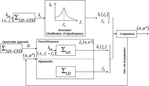
Figure 2 Schematic representation of the Venturi geometry (left) and meridian view of the Francis turbine (right)

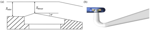
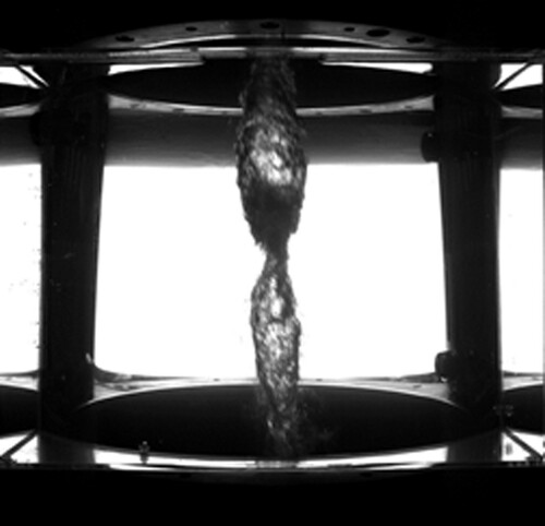
Figure 3 Experimental visualization of the cavitating vortex rope downstream the runner outlet

First, the mass flow gain factor ${\chi }_1$ is determined by following a quasi-static approach: at least six CFD simulations are performed by keeping constant the pressure just downstream the cavitation volume for different inlet discharges, which requires the outlet pressure to be adjusted. The variation of the cavitation volume as a function of the inlet discharge gives the mass flow gain factor.

Then, a global optimization process is performed to derive both the wave speed a and the second viscosity parameters ${\mu }^{\mathrm{\prime }\mathrm{\prime }}$. In this optimization process, both CFD and 1-D system responses to a fluctuating outlet static pressure are compared. The set of parameters of the 1-D model is optimized to get the best fitting between the two system responses. By imposing outlet pressure fluctuations in a range of frequencies to the CFD model, the resonance frequency f_p of the system is identified when the maximum of cavitation volume and pressure fluctuations are experienced. Two quantities measured in the CFD domain are then considered as the objectives for the optimization process: the resonance frequency f_p of the system and the pressure fluctuation amplitudes at a given location ${\tilde{h}}_x$. The optimization process, searching the set of 1-D cavitation parameters, computes both the eigenfrequency and the forced response in the frequency domain of the 1-D model. By minimizing the errors for the two objectives between the 1-D and the CFD models, the set of 1-D cavitation parameters is found.

5 Test cases

Two test cases are considered: a 2-D Venturi and a simplified 3-D Francis turbine at model scale (Fig. 2).

The Venturi geometry is a convergent/divergent nozzle that has been studied experimentally and numerically at the LEGI laboratory (Barre et al., 2009) for an operating point defined by an inlet velocity C_inlet = 10.8 m s⁻¹ (which corresponds to an inlet flow rate of Q_inlet = 0.024 m³ s⁻¹) and an inlet pressure p_inlet = 36000 Pa. The convergence angle is equal to 4.3° (with a sharp edge upstream the throat) whereas the divergence angle downstream the throat is equal to 4°. The top wall is straight. The inlet section is 50 × 44 mm² large whereas at the throat the section is reduced to 43.7 × 44 mm². The cavitation sheet extends downstream the throat with a length smoothly fluctuating between 70 mm and 85 mm.

A reduced scale model test of the Francis turbine has been performed to investigate part load (Favrel et al., 2015) and full load (Müller et al., 2016) operating conditions. The full load operating point considered in the present study is defined by a specific speed ν, a discharge factor Q_ED, a speed factor n_ED and a Thoma number σ, whose values are gathered in Table 1 and expressions are given in Eqs (15) to (18): (15) $\begin{array}{rl}\nu & =\frac{\omega }{2^{3/4}{\pi }^{1/2}}\frac{Q^{1/2}}{E^{3/4}}\end{array}$(15) (16) $\begin{array}{rl}{Q}_{ED}& =\frac{Q}{D^2{E}^{1/2}}\end{array}$(16) (17) $\begin{array}{rl}{n}_{ED}& =\frac{nD}{E^{1/2}}\end{array}$(17) (18) $\begin{array}{rl}\sigma & =\frac{NPSE}{E}\end{array}$(18) where ω is the rotating speed (rad s⁻¹), Q the flow discharge (m³ s⁻¹), E the specific energy (m² s⁻²), D the outlet runner diameter (m) and NPSE the net positive suction energy (m² s⁻²).

Table 1 Values of the parameters defining the operating point of the Francis turbine test case

Operating points	ν (–)	QED (–)	nED (–)	σ (–)
OP1	0.310	0.260	0.288	0.200

For this configuration, a quasi-stable cavitating vortex rope is observed downstream the runner outlet (Fig. 3).

6 2-D Venturi

6.1 CFD numerical set-up

The CFD simulations are performed by using the software Ansys CFX v15.0 (Ansys Inc., Canonsburg, USA). The computational domain (Fig. 4a) is extended downstream the cavitation sheet to avoid the interaction between the cavitation sheet and the outlet boundary condition. The structured mesh (Fig. 4b) contains 15,000 nodes. The y⁺ averaged value is close to 50 and the maximum value does not exceed 100. No mesh influence has been carried out. The mesh is generated based on the authors experience (see for instance Goncalves & Decaix, 2012 for a mesh influence study). The saturated pressure is set to 2300 Pa according to Goncalves and Patella (2009).

Figure 4 Computational domain of the 2-D Venturi (a) and view of the mesh at the throat (b)

The boundary conditions set are the inlet velocity C_in and the outlet pressure p_outlet. A no-slip wall condition is imposed at the top and bottom walls. In addition, the turbulent stresses in the first cell close to the wall are computed using a wall law. The convective terms are discretized with a high-order scheme for the momentum equation and an upwind first order scheme for the equations for k and ω. The transport equation for the vapour volume fraction and the momentum conservation equation are solved in a segregated manner. For the unsteady simulations, an implicit second order backward scheme is used with a time step set to 2 × 10⁻⁴ s (with five internal coefficient loops) allowing the RMS of the CFL number to be lower than 3. An unsteady simulation requires approximately 30 CPU hours.

6.2 1-D SIMSEN transient simulations

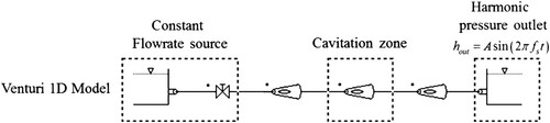
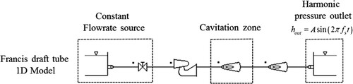
The Venturi is modelled with the SIMSEN software (Power Vision Engineering, CH-1025 St-Sulpice, Switzerland), which includes the cavitation model described previously (Fig. 1). The cavitation zone is spatially discretized with a lumped model. In the cavitation free region, the wave speed is set to 1000 m s⁻¹. Finally, the boundary conditions of the 2-D model are reproduced in the 1-D model: a constant discharge source at the inlet and a sinusoidal static pressure at the outlet (Fig. 5).

Figure 5 1-D transient models solved with the SIMSEN software. Venturi test case

6.3 CFD simulations results

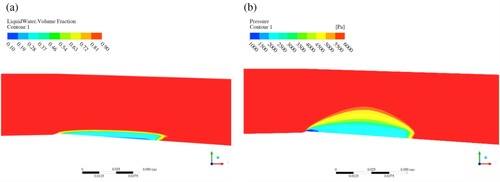
For the experimental inlet velocity, the outlet pressure is set to get a cavitation sheet that extends 70 mm downstream the throat. Figure 6 shows the contours of the liquid volume fraction downstream the throat. As observed experimentally, the cavitation sheet extends approximately 70 mm downstream the throat. Contrary to the experiment, the cavity is steady, no re-entrant jet is observed in the closure part of the cavity. The inlet pressure is equal to p_inlet = 33,000 Pa which is close to the 36,000 Pa measured experimentally. The difference can be due to the inability of the simulation to properly simulate the unsteadiness of the cavity closure (Barre et al., 2009).

Figure 6 Contours of the liquid volume fraction (a) and the pressure (b) downstream the throat. 2-D Venturi test case. CFD results at the experimental boundary conditions

6.4 Identification of mass flow gain factor parameter

As previously described in Section 4, the identification of the mass flow gain factor required the simulation of seven different couples of inlet velocity C_inlet and outlet pressure p_outlet boundary conditions. For all couples (C_inlet; p_outlet), the pressure downstream the cavitation sheet (plane 3 in Fig. 4a) is kept constant. Expressed in a dimensionless piezometric head defined as: h* = p/(0.5 ρ C_ref²) with C_ref = 10.8 m s⁻¹; the pressure value in plane 3 is: $h_3^{\ast }=0.41$.

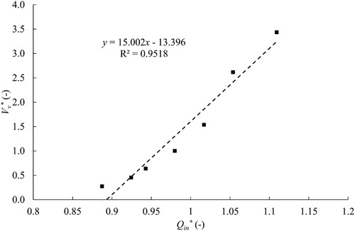
The values of the dimensionless vapour volume in the cavity against the dimensionless inlet discharge are plotted in Fig. 7. The dimensionless vapour volume is computed by dividing the volume of vapour by the reference volume of vapour V_ref = 0.0002 m³ obtained for the experimental boundary conditions. The reference flow discharge Q_ref is equal to 0.024 m³ s⁻¹. The linear regression carries out on the data plotted in Fig. 7 gives a slope of 15 that can be identified as a dimensionless mass flow gain factor following Eq. (13). The corresponding physical value ${\chi }_1=-0.001$ s of the mass flow gain factor is computed using V_ref and Q_ref.

Figure 7 Evolution of the dimensionless cavitation volume versus the dimensionless discharge keeping the pressure at plane 3 constant. 2-D Venturi test case, CFD results

6.5 Identification of the wave speed and second viscosity parameters

The determination of the wave speed a and the second viscosity ${\mu }^{\mathrm{\prime }\mathrm{\prime }}$ is done by performing five CFD simulations with a constant inlet flow discharge and a sinusoidal pressure outlet. The inlet flow discharge is set to Q_inlet = Q_ref = 0.024 m³ s⁻¹, whereas the outlet pressure expresses in dimensionless piezometric head is: (19) $h_{out}^{\ast }=h_{ref}^{\ast }+h_a^{\ast }\sin \left(2\pi ft\right)$(19) with $h_{ref}^{\ast }$ = 1.22, $h_a^{\ast }$ = 0.034 and f the imposed frequency. Five different frequencies have been considered: 0.5, 1.4, 2, 4 and 10 Hz.

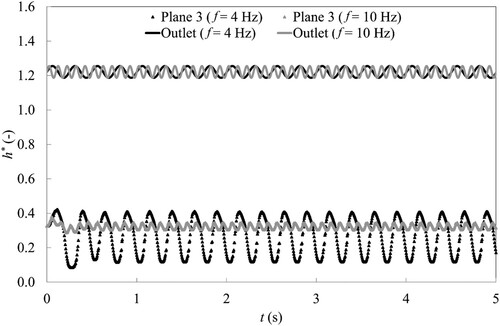
The time-history of the dimensionless piezometric head at the outlet section and at plane 3 are plotted respectively in Figs 8 and 9. Depending on the simulation, between five and 50 periods have been acquired. The shape of the signal at plane 3 depends strongly on the excitation frequency imposed at the outlet. For the low frequency of 0.5 Hz, the shape of the signal at plane 3 is sinusoidal with an amplitude five times higher. For the frequency of 1.4 Hz and 2 Hz, the shape of the signal at plane 3 is no longer sinusoidal and shows peaks, which is typical of resonance conditions. The amplitude of the signal is around nine times higher than the amplitude imposed at the outlet. Beyond a frequency of 2 Hz, the sinusoidal shape of the signal at plane 3 is recovered. Furthermore, for the frequency of 10 Hz, the amplitude of the signal at plane 3 is smaller than the excitation amplitude imposed at the outlet. From these observations, the cavitation sheet present two behaviours: for low frequency, it behaves like an amplifier, whereas for higher frequencies it acts as a damper. The resonance frequency is close to the frequency of 2 Hz.

Figure 8 Time-history of the dimensionless piezometric head signal at the outlet and plane 3 for f = 0.5 Hz, f = 1.4 Hz and f = 2 Hz. 2-D Venturi test case, CFD results

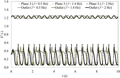
Figure 9 Time-history of the dimensionless piezometric head signal at the outlet and plane 3 for f = 4 Hz and f = 10 Hz. 2-D Venturi test case, CFD results

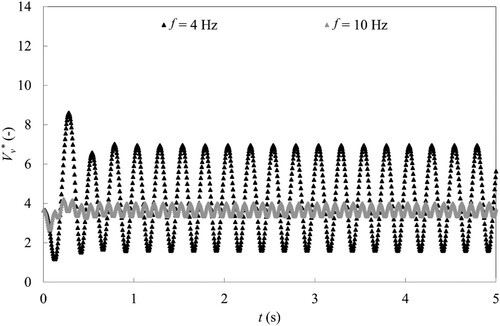
The time-history of the dimensionless vapour volume in the cavity is shown in Figs 10 and 11. As for the dimensionless piezometric head, the vapour volume signal is sinusoidal for the frequencies of 0.5 Hz, 4 Hz and 10 Hz, whereas for the frequencies of 1.4 and 2 Hz, the signal is no more sinusoidal. It is noticeable that for the frequency of 2 Hz, the volume of vapour reaches values close to zero, which means that the cavitation sheet collapses.

Figure 10 Time history of the dimensionless volume of vapour for f = 0.5 Hz, f = 1.4 Hz and f = 2 Hz. 2-D Venturi, CFD results

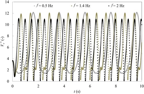
Figure 11 Time history of the dimensionless volume of vapour for f = 4 Hz and f = 10 Hz. 2-D Venturi, CFD results

Based on the unsteady CFD simulation, the identification of the wave speed a and the second viscosity ${\mu }^{\mathrm{\prime }\mathrm{\prime }}$ is performed by setting the resonance frequency f_n and the amplitude of the pressure fluctuations h* at plane 2 (Fig. 4) as the objective functions of the global optimization. Two identifications have been performed with and without the mass flow gain factor to assess its influence on the wave speed and the second viscosity values. With ${\chi }_1$ = −0.001 s, the identification procedure leads to a = 4.3 m s⁻¹ and ${\mu }^{\mathrm{\prime }\mathrm{\prime }}$ = 800 Pa s. 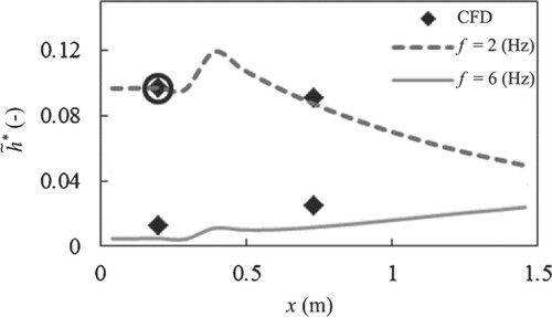By ignoring the mass flow gain factor, the identification procedure leads to a = 4.3 m s⁻¹ and ${\mu }^{\mathrm{\prime }\mathrm{\prime }}$ = 790 Pa s. Therefore, the low value of the mass flow gain factor barely influences the parameters. In Fig. 12, the forced response of the 1-D model is plotted along the system abscissa with also the CFD simulation results at plane 2 and plane 4. At the resonance conditions (circled symbol), for which the identification process has been carried out, the 1-D model matches the CFD simulation results. At other operating conditions, a difference is observed between the 1-D model and the CFD simulations. This difference observed for out of resonance conditions could be explained by either frequency dependent cavitation parameters or non-linearities of the system at the resonance conditions.

Figure 12 Forced response of the system for two different frequencies obtained with the 1-D transient simulation. 2-D Venturi test case. The circle point refers to the resonance condition for which the identification process has been carried out

7 3-D Francis turbine

7.1 CFD numerical set-up

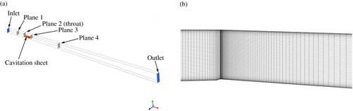
For the 3-D Francis turbine, the computational domain is simplified compared to the whole machine and consists only of the runner, the draft tube cone and a straight draft tube extension as shown in Fig. 13a. The runner and the cone domains are meshed with structured hexahedra mesh, whereas an unstructured tetrahedral mesh is used for the draft tube extension to enhance the dissipation of the vortex rope preventing numerical instabilities if the cavitation volume interacts with the boundary conditions (Fig. 13b). The total number of nodes is close to 4.5 million with 2.5 million of nodes in the runner domain. The averaged y⁺ value is of 20 and the maximum value does not exceed 60. The influence of the mesh is discussed in Decaix et al. (2017). The saturated pressure is set to 1800 Pa according to the experiment.

Figure 13 Computational domain of the 3-D Francis turbine (a) and associated mesh in a meridional plane (b)

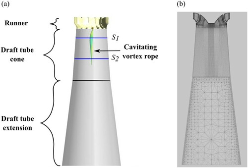
Figure 14 1-D transient models solved with the SIMSEN software. Francis turbine test case

The velocity field is imposed at the runner inlet. This field is extracted from a single phase CFD simulation on the full turbine domain including all the components from the spiral case to the draft tube outlet. The pressure is set at the outlet section by imposing a sinusoidal signal. No-slip wall condition is set at the solid walls. The turbulent stresses in the first cell close to the walls are computed using a wall law. The convective terms are discretized with a high-order scheme for the mean field and an upwind first order scheme for the turbulent field. The transport equation for the vapour volume fraction and the momentum conservation equation are solved in a segregated manner. For the unsteady simulations, an implicit second order backward scheme is used with a time step set to 2 × 10⁻⁴ s (with five internal coefficient loops), allowing the RMS of the CFL number to be lower than 3. An unsteady simulation requires between 10,000 and 15,000 CPU hours.

7.2 1-D SIMSEN transient simulations

The 1-D model of the Francis turbine test case is solved with the SIMSEN software which includes the cavitation model described previously (Fig. 14). The cavitation zone, where cavitation parameters must be identified, is spatially discretized with a distributed model. In the cavitation free region, the wave speed is set to 1000 m s⁻¹ (according to eq. 2.20 in Nicolet, 2007). Finally, the boundary conditions of the 3-D model are reproduced in the 1-D model: a constant discharge source at the inlet and a sinusoidal static pressure at the outlet.

7.3 CFD simulations results

A preliminary simulation is carried out with a static outlet pressure. This operating point corresponds to a stable vortex rope. To compare the experiment with the simulation, the parameter σ_U, representing a local cavitation (Thoma) number and defined by Eq. (20), is computed in the two sections S₁ and S₂ located in the draft tube cone (Fig. 13a): (20) ${\sigma }_U=\frac{p_{ref}-p_v}{\frac{1}{2}\rho U\frac{2}{1}}$(20) where p_ref is the mean pressure in the section considered, p_v the vapour pressure set to 1800 Pa and $U_{\overline{1}}$ the rotating velocity at the outer diameter at the runner outlet. The experimental and the numerical value of the parameter σ_U in the two sections of the draft tube cone are given in Table 2. The differences between the experimental and the numerical values are lower than 1%. Additional comparisons with the experimental data are available in Decaix et al. (2015b, 2017) such as the comparison of the velocity profiles in the cone.

7.4 Identification of the mass flow gain factor parameter

As for the Venturi test case, the mass flow gain factor is determined by computing six two-phase steady state computations, for which the inlet flow rate and the outlet pressure are modified to keep the pressure at the interface between the structured and unstructured mesh constant. Expressed in the dimensionless piezometric head defined as: h* = p/(0.5 ρ C_ref²) with C_ref = 14.7 m s⁻¹; the pressure at this location is: $h_{int}^{\ast }=0.5$.

The values of the dimensionless vapour volume $V_v^{\ast }$ = V_v/V_ref in the cavity versus the dimensionless inlet discharge is plotted in Fig. 15. The reference vapour volume V_ref = 0.06 m³ and the reference flow discharge Q_ref = 0.516 m³ s⁻¹ correspond to the values obtained for the experimental boundary conditions. The vapour volume evolves linearly with the inlet flow rate. By applying the same procedure than for the Venturi test case, the mass flow gain factor can be computed: ${\chi }_1$ = −0.034 s. For very low volume of vapour, the agreement with the linear approximation is questionable. However, for such low volume of vapour only few cells are filled of vapour and the accuracy of the simulation is also questionable. In the present study no investigation of the influence of low volumes of vapour on the results has been carried out.

7.5 Identification of the wave speed and second viscosity parameters

The determination of the wave speed a and the second viscosity ${\mu }^{\mathrm{\prime }\mathrm{\prime }}$ is performed following the same methodology as for the Venturi test case. Therefore, a sinusoidal pressure is imposed at the outlet section expressed by Eq. (19), with $h_{ref}^{\ast }$ = 0.65, $h_a^{\ast }$ = 0.047 and f the frequency imposed. Four different frequencies have been considered: 10, 20, 30 and 50 Hz. For the frequency of 20 Hz, the simulation is performed with a lower amplitude $h_a^{\ast }$ = 0.037 to avoid numerical instability. For each simulation, one second of physical time has been computed.

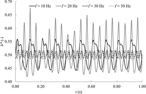
The time-history of the dimensionless piezometric head at the outlet section and at the interface is plotted respectively in Figs 16 and 17. For the frequencies of 30 and 50 Hz, the piezometric head fluctuations are smaller at the interface than at the outlet section. It is the opposite for the frequency of 10 and 20 Hz. Furthermore, for the frequency of 20 Hz, the sinusoidal shape of the outlet signal is lost at the interface, whereas it is close to be recovered for the frequency of 10 Hz.

Table 2 Values of the σ_U parameter in the two sections of the draft tube

Section	Experiment	CFD
S1	0.43	0.43
S2	0.47	0.48

Figure 15 Evolution of the dimensionless cavitation volume versus the dimensionless discharge keeping the pressure at the domain interface constant. Francis turbine test case, CFD results

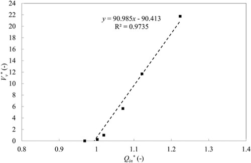
Figure 16 Time-history of the dimensionless piezometric head signal at the outlet. Francis turbine test case, CFD results

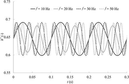
Figure 17 Time-history of the dimensionless piezometric head signal at the interface. Francis turbine, CFD results

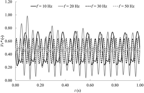
The time-history of the dimensionless volume of vapour for each frequency is shown in Fig. 18. The volume of vapour fluctuates slightly for the frequency of 50 Hz. The fluctuations are the largest for the frequency of 20 Hz, with a minimum value near zero, which means that the vortex rope is close to collapse.

Figure 18 Time-history of the dimensionless volume of vapour. Francis turbine test case, CFD results

Based on the unsteady CFD simulations, the identification of the wave speed a and the second viscosity ${\mu }^{\mathrm{\prime }\mathrm{\prime }}$ is performed by setting the resonance frequency f_n and the amplitude of the pressure fluctuations h* at the interface between the draft tube cone and its extension (Fig. 13) as the objective functions of the global optimization process. Two identifications have been performed with and without the mass flow gain factor to assess its influence on the wave speed and the second viscosity values. With ${\chi }_1$ = −0.034 s, the identification procedure leads to a = 85.8 m s⁻¹ and ${\mu }^{\mathrm{\prime }\mathrm{\prime }}$ = 17,723 Pa s. 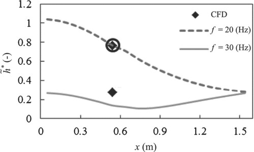By ignoring the mass flow gain factor, the identification procedure leads to a = 81 m s⁻¹ and ${\mu }^{\mathrm{\prime }\mathrm{\prime }}$ = 16,280 Pa s. Since the mass flow gain factor has a stabilizing effect, to keep the same eigenfrequency, the value of the wave speed parameter is increased with the second viscosity. In Fig. 19, the forced response of the 1-D model is plotted along the system abscissa with also the CFD simulation results at the interface. At the resonance conditions (circled symbol), for which the identification process has been carried out, the 1-D model matches the CFD simulation results. At the other operating conditions, a difference is observed between the 1-D model and the CFD simulations. As for the Venturi test case, the difference could be explained by either frequency dependent cavitation parameters or nonlinearities of the system at the resonance conditions.

Figure 19 Forced response of the system for two different frequencies obtained with the 1-D transient simulations. Francis turbine test case. The circle point refers to the resonance condition for which the identification process has been carried out

8 Summary

The identification procedure of the parameters of the 1D transient model has been carried out for two different cavitating flows: a 2D Venturi and a 3D Francis turbine. For each case study, the identified parameters are gathered in Table 3 and split into two sets depending whether or not the mass flow gain factor is accounted for. For the Venturi test case, the accounted for the mass flow gain factor, which features a small value, does not influence the value of the wave speed and change the value of the second viscosity by less than 1.5%. For the Francis turbine test case, the influence of the mass flow gain factor is stronger, with a difference of 6% on the wave speed and 9% on the second viscosity.

Table 3 Values of the identified parameter for both test cases

	Venturi	Francis turbine
With χ1	a = 4.3 m s^−1µ^″ = 800 Pa sχ1 = −0.001 s	a = 85.8 m s^−1µ^″ = 17,723 Pa sχ1 = −0.034 s
Without χ1	a = 4.3 m s^−1µ^″ = 790 Pa s	a = 81 m s^−1µ^″ = 16,280 Pa s

9 Conclusion

1-D transient models used to perform stability analyses of power plant require the calibration of three parameters (the mass flow gain factor ${\chi }_1$, the wave speed a and the second viscosity ${\mu }^{\mathrm{\prime }\mathrm{\prime }}$) when the analyses deal with the presence of a cavitating vortex rope in the draft tube of a Francis turbine. The identification of these parameters can be achieved using either measurements or CFD data. In this paper, a methodology using steady and unsteady RANS simulations is described. The identification of the mass flow gain factor is carried out by performing seven steady simulations for seven different coupled inlet flow rate and outlet pressure boundary conditions, which gives a relation of the cavitation volume as a function of the inlet flow rate. The slope of the relation corresponds to the mass flow gain factor. The identification of both the wave speed and the second viscosity parameters is obtained from unsteady 3-D simulations for which a sinusoidal outlet pressure is imposed. The frequency and the amplitude of the pressure at the resonance conditions are used as objective functions for the identification of the 1-D model parameters.

This procedure has been applied successfully to two different test cases: a 2-D Venturi geometry characterized by an attached cavitation sheet and a 3-D cavitating vortex rope that develops in the cone of the draft tube of a Francis turbine.

The results show a range of possible values for the three parameters (the mass flow gain factor ${\chi }_1$, the wave speed a and the second viscosity ${\mu }^{\mathrm{\prime }\mathrm{\prime }}$) that covers one order of magnitude, which means that the values of the parameters are strongly related to the flow considered.

The comparison of the 1-D model and the CFD simulations for operating points at out of the resonance frequency makes appear differences. Additional investigations are therefore required to provide an explanation to these observations.

Notation

a	=	sound speed (m s−1)
Cc	=	cavitation compliance (m2)
${\mathit{C}}_{\mathit{m}}$	=	velocity vector (m s−1)
h	=	piezometric head (m)
Q	=	flow discharge (m3 s−1)
p	=	pressure (Pa)
t	=	time (s)
Vc	=	volume of vapour (m3)
αv	=	vapour volume fraction (–)
μ	=	dynamic viscosity (Pa s−1)
μt	=	turbulent dynamic viscosity (Pa s−1)
μ″	=	second viscosity (Pa s−1)
ρ	=	density (kg m−3)
$\mathit{\tau }$	=	viscous stress tensor (Pa)
$\mathit{\tau }$t	=	turbulent stress tensor (Pa)
χ	=	mass flow gain factor (s)

Additional information

Funding

The research leading to the results published in this paper is part of the HYPERBOLE research project, granted by the European Commission (ERC/FP7-ENERGY-2013-1-Grant 608532); European Research Council.

References

- Alligné, S., Decaix, J., Nicolet, C., Avellan, F., & Münch, C. (2015). Identification of the wave speed and the second viscosity in cavitating flow with 2D RANS computations – Part II. Journal of Physics: Conference Series, 656, 012057. doi:https://doi.org/10.1088/1742-6596/656/1/012057
- Alligné, S., Nicolet, C., Tsujimoto, Y., & Avellan, F. (2014). Cavitation Surge Modelling in Francis Turbine Draft Tube. Journal of Hydraulic Research, 52(3), 399–411. doi:https://doi.org/10.1080/00221686.2013.854847
- Alligneé, S., Nicolet, C., & Avellan, F. (2011). Identification of Francis turbine helical vortex rope excitation by CFD and resonance simulation with the hydraulic system. In ASME-JSME-KSME Joint Fluids Engineering Conference, July 24–29. ASMEDC. doi:https://doi.org/10.1115/ajk2011-06089
- Bakir, F., Rey, R., Gerber, A., Belamri, T., & Hutchinson, B. (2004). Numerical and experimental investigations of the cavitating behavior of an inducer. The International Journal of Rotating Machinery, 10(1), 15–25. doi:https://doi.org/10.1155/S1023621X04000028
- Barre, S., Rolland, J., Boitel, G., Goncalves, E., & Patella, R. F. (2009). Experiments and modeling of cavitating flows in Venturi: Attached sheet cavitation. European Journal of Mechanics – B/Fluids, 28(3), 444–464. doi:https://doi.org/10.1016/j.euromechflu.2008.09.001
- Brennen, C. (1995). Cavitation and bubble dynamics. Oxford University Press.
- Brennen, C., & Acosta, A. (1973). Theoretical, quasistatic analysis of cavitation compliance in turbopumps. Journal of Spacecraft and Rockets, 10(3), 175–180. doi:https://doi.org/10.2514/3.27748
- Chen, C., Nicolet, C., Yonezawa, K., Farhat, M., Avellan, F., & Tsujimoto, Y. (2008). One-dimensional analysis of full load draft tube surge. Journal of Fluids Engineering, 130(4), 041106. doi:https://doi.org/10.1115/1.2903475
- Decaix, J., Alligné, S., Nicolet, C., Avellan, F., & Münch, C. (2015a). Identification of the wave speed and the second viscosity of cavitation flows with 2D RANS computations – Part I. Journal of Physics: Conference Series, 656, 012060. doi:https://doi.org/10.1088/1742-6596/656/1/012060
- Decaix, J., Müller, A., Avellan, F., & Münch, C. (2015b). Rans computations of a cavitating vortex rope at full load. 6th IAHR International Meeting of the Workgroup on Cavitation and Dynamic Problems in Hydraulic Machinery and Systems, September 9–11, Lubjana, Slovenia.
- Decaix, J., Müller, A., Favrel, A., Avellan, F., & Münch, C. (2017). URANS models for the simulation of full load pressure surge in Francis turbines validated by particle image Velocimetry. Journal of Fluids Engineering, 139(12). doi:https://doi.org/10.1115/1.4037278
- Dörfler, P. (1982). System dynamics of the Francis turbine half load surge. Proceedings of the IAHR Symposium on Operating Problems of Pump Stations and Powerplants, September 13–17, Amsterdam, Netherlands.
- Dorfler, P., Keller, M., & Braun, O. (2010). Fancis full-load surge mechanism identified by unsteady 2-phase CFD. 25th IARH Symposium on Hydraulic Machinery and Systems, September 20–24 (pp. 1–10). IOP Conf. Series: Earth and Environmental Science.
- Favrel, A., Müller, A., Landry, C., Yamamoto, K., & Avellan, F. (2015). Study of the vortex-induced pressure excitation source in a Francis turbine draft tube by particle image velocimetry. Experiments in Fluids, 56(12), 215. doi:https://doi.org/10.1007/s00348-015-2085-5
- Ghahremani, F. (1971). Pump cavitation compliance. In Proceedings of Cavitation forum ASME, May 10–12 (pp. 1–3). New York, USA.
- Goncalves, E., & Decaix, J. (2012). Wall model and mesh influence study for partial cavities. European Journal of Mechanics – B/Fluids, 31, 12–29. doi:https://doi.org/10.1016/j.euromechflu.2011.08.002
- Goncalves, E., & Patella, R. F. (2009). Numerical simulation of cavitating flows with homogeneous models. Computers & Fluids, 38(9), 1682–1696. doi:https://doi.org/10.1016/j.compfluid.2009.03.001
- Ji, B., Luo, X. W., Arndt, R. E., Peng, X., & Wu, Y. (2015). Large Eddy Simulation and theoretical investigations of the transient cavitating vortical flow structure around a NACA66 hydrofoil. International Journal of Multiphase Flow, 68, 121–134. doi:https://doi.org/10.1016/j.ijmultiphaseflow.2014.10.008
- Koutnik, J., Nicolet, C., Schohl, G., & Avellan, F. (2006). Overload surge event in a pumped-storage power plant. 23rd IAHR Symposium on Hydraulic Machinery and Systems, October 17–21, 1, 1–15.
- Landry, C., Favrel, A., Müller, A., Nicolet, C., & Avellan, F. (2016). Local wave speed and bulk flow viscosity in Francis turbines at part load operation. Journal of Hydraulic Research, 54(2), 185–196. doi:https://doi.org/10.1080/00221686.2015.1131204
- Menter, F. R. (2009). Review of the shear-stress transport turbulence model experience from an industrial perspective. International Journal of Computational Fluid Dynamics, 23(4), 305–316. doi:https://doi.org/10.1080/10618560902773387
- Müller, A., Favrel, A., Landry, C., & Avellan, F. (2017). Fluid–structure interaction mechanisms leading to dangerous power swings in Francis turbines at full load. Journal of Fluids and Structures, 69, 56–71. doi:https://doi.org/10.1016/j.jfluidstructs.2016.11.018
- Müller, A., Yamamoto, K., Alligné, S., Yonezawa, K., Tsujimoto, Y., & Avellan, F. (2016). Measurement of the Self-Oscillating Vortex Rope Dynamics for Hydroacoustic Stability Analysis. Journal of Fluids Engineering, 138(2), 021206. doi:https://doi.org/10.1115/1.4031778
- Nicolet, C. (2007). Hydroacoustic Modelling and Numerical Simulation of Unsteady Operation of HydroelectricSystems [Ph.D. dissertation]. ÉCOLE POLYTECHNIQUE FÉDÉRALE DE LAUSANNE. https://infoscience.epfl.ch/record/98534?ln=en
- Pezzinga, G. (2003). Second viscosity in transient cavitating pipe flows. Journal of Hydraulic Research, 41(6), 656–665. doi:https://doi.org/10.1080/00221680309506898
- Zwart, P., Gerber, A., & Belamri, T. (2004). A two-phase flow model for predicting cavitation dynamics. Fifth International Conference on Multiphase Flow, Yokohama, Japan, May 30–June 3, 152.