Time reversal of waves in hydraulics: experimental and theoretical proof with applications

Abstract

Time reversal of waves is an intriguing wave property that underpins a breadth of applications in physics and engineering. Waves contain information about their sources and the media through which they propagate. Thus, time reversal of measured wave signals has the potential of localizing and characterizing wave sources and of inferring the properties of the medium. Herein, we experimentally demonstrate the time reversibility of acoustic waves propagating in water-filled viscoelastic high-density polyethylene (HDPE) pipes. Evidently, the two mechanisms that restrict time reversal are the stability of wave paths to perturbations and damping. Perturbations, however, are found to grow slowly in time (∼t^1/2) and are not critical for the time reversal of waves. To evaluate the effect of damping, we perform an order of magnitude analysis on the non-reversible terms of the coupled waveguide momentum equations and derive a dimensionless time reversal parameter TR showing that damping develops linearly with time (i.e. TR ∼ t). Subsequently, we apply the TR parameter to our experiments and relevant experimental proofs from the literature to find that the time reversal of waves only holds for TR ∼ 1 or less; hence providing a criterion to estimate the range over which time reversal-based wave techniques and methodologies are valid. Finally, we discuss the various existing applications of time reversal in hydro-environmental research and engineering and anticipate that the presented work will stimulate further development.

Keywords:

• Fluid-filled pipes
• gravity waves
• instabilities
• pressure waves
• scale analysis
• time reversal
• viscous damping

1 Introduction

There is no unique definition of time reversal. Here, we limit ourselves to processes that can experimentally be proven time reversible in the following sense: a source located at x_s emits a pulse at time t = 0 that propagates through a medium. Receiving transducers, positioned at a distance from the source, sample the incoming wave for a total time duration T_tot. The received signals are time reversed (last in, first out) and reemitted. If the wave refocuses at the original source location after time T_tot, then the process is deemed time reversible. A fascinating experiment that fits the stated definition is a classic problem in hydraulics and involves the time reversal of gravity waves (de Mello et al., 2016; a video of this experiment can be found here: https://www.youtube.com/watch?v=XDbLi2YGQn8). There, an object is dropped on the calm surface of the pool, creating concentric ripples that propagate from its entry point. The pool walls comprise of multiple paddles that each can independently sample the height of the water surface. During this particular experiment and until waves die out, only the paddles positioned along two opposing pool walls are in operation. In the time reversal stage, the same paddles actively transmit the time reversed waveform acquired during the initial (forward) stage. At first, the time-reversed wave field on the surface of the pool appears random and chaotic; with time, however, the circular ripple pattern re-emerges, and the waves refocus at the location of the original disturbance. Another ingenious series of experiments that visualize time reversal is presented in Heaton et al. (2017) where the authors employ elastic waves propagating in an aluminium plate. In one set of experiments, a number of Lego figurines is placed on top of the plate during the time reversal stage. As the vertical displacement field refocuses, only the figurine located above a preselected focal point is overturned, while the others remain unaffected.

Time reversal is far from a theoretical endeavour; in fact, it forms the foundation of many technologies. If you happen to be reading this manuscript on an electronic device equipped with a touch screen, you are likely to be experiencing time reversal at work. Indeed, some touch and tactile screens are based on the ability of time reversal to refocus wave energy at specific points to recognize touch inputs and provide haptic feedback (Hudin et al., 2015). Another practical application of time reversal mirrors is pulse-echo defect detection employed in several fields, including the medical imaging and treatment of brain tumours (Thomas & Fink, 1996) and kidney stones (Thomas et al., 1996), ultrasonic non-destructive testing of solid materials (Chakroun et al., 1995), and underwater acoustics for locating targets (Li et al., 2011). Considering the scenario of waveguide containing a defect, an acoustic pulse is injected to “illuminate” the domain. The defect is subsequently turned into a passive acoustic source as the pulse is scattered off its surface due to the apparent impedance discontinuity. By capturing that reflection, time reversal techniques are employed to uniquely focus the distorted signal at the location of the defect. In pipe systems, the methods applied in Wang and Ghidaoui (2018) and Zouari et al. (2019) implicitly show that the time reversed response is key for the precise localization and characterization of defects.

The degree of temporal compression of the recreated pulse at the location of the original source increases with the number of transducers that capture the signal, as well as in the presence of reflective boundaries and inhomogeneities. For instance, in Roux and Fink (2000), Roux et al. (1997) and Tanter et al. (1998) the performance of time reversal in a fluid waveguide bounded by non-absorbing symmetric walls was found superior to that in free field. Multiple works (e.g. Derode et al., 1995; Draeger & Fink, 1997) have also shown that the time reversal process is enhanced under the presence of multiple scatterers or in non-dissipating reverberating chaotic cavities, where a single-channel time reversal mirror (i.e. a single receiving and reemitting transducer) was shown to be adequate. Theoretically, if the energy emitted from the source is acquired at its entirety, the source is then placed in a spot not smaller than half the probing wavelength, a value that corresponds to the diffraction limit (Cassereau & Fink, 1992). Nonetheless, researchers have been able to overcome this limit by including sub-wavelength scatterers (so-called metamaterials) in the propagating media and attain super-resolution (Blomgren et al., 2002; Fink, 2008; Lerosey et al., 2006).

Recently, the Smart Urban Water Supply Systems (SUWSS) project (Smart UWWS Team, 2017) proposed the use of acoustic waves for the condition assessment of pipe systems. Pressure waves in the low frequency regime with wavelengths much larger than the pipe diameter propagate over long distances (in the order of km) and provide a rough assessment of the network condition. Once a problematic segment is identified, high frequency pressure waves are used to pinpoint the location of the defect to within a few centimetres. Although the use of high-frequency waves with wavelengths comparable to the pipe diameter for the probing of water supply systems is a relatively new application, many researchers (Baik et al., 2013; Biot, 1952; Del Grosso, 1971; Grigoropoulos et al., 2018; Lin & Morgan, 1956; Louati & Ghidaoui, 2017) have shown that high-frequency wave propagation through such bounded waveguides is a dispersive phenomenon. For example, when a high-frequency point-like acoustic source is introduced inside a pipe, the transmitted waves propagate in all directions and bounce off the pipe boundaries. As a result, a receiver located at a distance records a signal that contains multiple reflections of the source emanating from the pipe walls. Waves that reflect at steeper angles from the pipe wall follow a longer path to the receiver, ultimately arriving at later times. The number of reflections (henceforth modes) created depends on the properties of the waveguide, the frequency bandwidth of the probing signal, as well as the radial location and physical dimensions of the source. A complete approach to the wave propagation in fluid-filled pipes must also include the description of the deformable pipe wall, further complicating the identification of a wave source or defect (i.e. a passive wave source) in such an environment.

Time reversal is a powerful tool that could resolve such complexities; however, its validity in the waveguide of interest must be proven. Jin et al. (2011) used piezoelectric transducers mounted on the outer pipe surface to show that ultrasonic guided waves in elastic steel pipes are time reversible. Herein, we present an experimental proof-of-concept of time reversal in water-filled viscoelastic HDPE pipes where the acoustic source is placed within the water. The signals employed have wavelengths comparable to the pipe radius and are, therefore, dispersed due to the radial boundaries giving rise to multiple propagating modes. Regardless, pure multipath propagation effects can successfully be compensated for by the time-reversal process (Roux et al., 1997). In contrast, an important condition for the full time-invariance property to hold is that the propagation medium is non-dissipative (Fink, 1997). However, fluid pressure (acoustic) waves propagating in HDPE pipes interact with the boundaries and are significantly attenuated due to the viscous properties of the material (Bergant et al., 2008). Besides, HDPE displays a nonlinear stress–strain relationship that depends on the applicable strain and strain rate, as well as the loading history under an oscillating load (Zhang & Moore, 1997). In effect, both wave speed and damping of waves propagating in fluid-filled HDPE pipes are frequency and mode dependent (Baik et al., 2010). In addition to the dissipative characteristics of the HDPE pipe wall, the effect of the fluid viscosity has to also be considered.

In fact, we demonstrate that the fundamental equations that describe the viscous fluid-filled HDPE pipe are inherently not time reversible. Nonetheless, the obtained experimental results indicate that time reversal under such settings is surprisingly robust. Moreover, the spatial focusing properties of time reversal are also experimentally verified on the same HDPE pipe set-up. Specifically, the time reversed pressure field is evaluated at multiple locations and is shown to uniquely refocus at the location of the original source. In light of these remarkable findings, we perform a comprehensive scale analysis based on the fundamental waveguide equations to elucidate the reasons time reversal holds despite the presence of damping. The outcome of this analysis is the time reversal parameter (TR), that corresponds to the ratio of viscous forces to the temporal acceleration. It is shown that as TR ∼ 1, the viscous losses in the considered system become significant, and the time reversibility of waves no longer holds. Subsequently, it is possible to estimate the applicable range for various time reversal applications given the characteristic scales of the system. More importantly, the validity of the time reversal parameter TR is general and, thus, not limited to pipeline applications. The fact is demonstrated by revisiting already published experimental results on time reversal of acoustic waves in the ocean and gravity waves on free-water surfaces, both documented in the non-hydraulics literature.

2 Time reversal experiments in HDPE pipes

2.1 Experimental set-up

The basis of the experimental set-up, located at the hydraulic lab at the Hong Kong University of Science and Technology (HKUST), is a straight 6.5 m long, DN80 HDPE pipe that connects two water-filled reservoirs at its ends. This set-up mimics real water supply systems where pipes are conduits and, thus, open to flow at both ends. The nominal internal diameter of the pipe is equal to D = 79.2 mm, while the pipe wall thickness h = 5.4 mm. The pipe runs uninterrupted along its length with its cross-section constant throughout, and water is quiescent. To minimize air entrainments, especially during the filling-up process of the system, the pipe is installed at a slight incline (1%). Even so, a piston-like block of fabric that completely occupies the pipe cross-sectional area is pulled along the length of the pipe several times to ensure that any air pockets are eliminated. This task is important, since contained air in the system lowers the expected wave speed and makes it pressure dependent. Moreover, air entrainments introduce acoustic reflectors that unpredictably alter the system response. The mechanical parameters of the coupled fluid-structure system, essential to estimate the compressional wave speed for each domain (i.e. fluid and structure), are presented in Table 1. Note that the calculated wave speeds shown in Table 1 are only relevant for waves with wavelengths much larger compared to the lateral dimensions of the waveguide. At increased frequencies, where wavelengths are of order of the pipe radius, propagating waves “bounce off” the pipe wall and follow a longer zigzag path that effectively reduces their wave speed.

Table 1 Mechanical characteristics of the two domains comprising the coupled waveguide

Fluid (water)
Bulk modulus, Kf	2.1 × 10^9 (kg m^–1 s^–2)
Density, ρf	1000 (kg m^–3)
Wave speed, cf = (Kf/ρf)^1/2	1450 (m s^–1)
Pipe (HDPE)
Young’s modulus, E	1.47 × 10^9 (kg m^–1 s^–2)
Poisson’s ratio, νp	0.43
Density, ρp	959 (kg m^–3)
Wave speed, cp = [E/ρp(1–νp^2)]^1/2	1372 (m s^–1)

Due to the prospect of utilizing time reversal techniques for defect identification in water supply pipelines, the portion of the pipe cross-section covered by transducers must be minimal to avoid obstructing the flow. In addition, the inaccessibility of water supply systems makes it difficult, if not impossible, to introduce multiple transducers. For these reasons, the experimental set-up is limited to a single-channel time reversal mirror. It must also be noted that the tested waveguide is semi-infinite (thus far from a closed cavity). In this setting, a single-channel time reversal set-up is at a disadvantage since a large part of the emitted wave energy escapes and cannot be reversed, with possible severe implications to the successful application of time reversal.

The point-like acoustic source is placed in the water and within the boundaries of the pipe wall at one end of the pipe, by means of a Brüel & Kjær (Nærum, Denmark) Type 8103 transducer. The transmitting voltage response (TVR) of the transducer at e.g. 35 kHz is rated equal to 112 dB re μPa/1 V @ 1 m by its manufacturer (Brüel & Kjær, 2019), while its input voltage V_rms is limited to 100 V. Utilizing these values, the maximum sound pressure level (SPL) at 1 m from the source may be calculated from: (1) $\text{SPL}=V_{rms}\left(\text{dB}\right)+\text{TVR}\left(f\right)$(1) where the V_rms(dB) scale is relative (re) to 1 V; thus: (2) $\text{SPL}=20{\log }_{10}\left(100\right)+112=152\mathrm{d}\mathrm{B}\mathrm{r}\mathrm{e}\mu \mathrm{P}\mathrm{a}$(2) or 4 mm of pressure head. The result of Eq. (2) indicates that the probing signal injected to the system is minute in magnitude compared to typical water-hammer waves and, thus, not a factor that could compromise the structural integrity of the pipeline. On the other hand, given that the frequency of the injected signals is much higher than potential high-amplitude background pressure fluctuations, it is possible to filter out these low frequency components without affecting the detectability of the signal of interest. To evaluate the response of the system to the injected signal, an identical receiving transducer is positioned at a distance equal to x = 2 m from the source, corresponding to approximately 25 times the pipe internal diameter (x/D = 25.3). The specific distance is selected so that the various modes propagating at different group velocities along the waveguide have adequate time to separate and become easily discernible at the receiver.

As regards to the radial direction, the emitting transducer (i.e. acoustic projector) is mounted at approximately the pipe centre via a 3D printed plastic resin base with an embedded magnet that forms a pair with another on the outer pipe surface (Fig. 1b). The aim is to keep the excited pressure wave field axisymmetric. As a result, the number of excited modes is manageable, and the obtained response is easier to interpret. It is stressed that the validity of time reversal is by no means depending on the symmetry, or lack thereof, of the pressure field. The magnetic mounting mechanism also allows for the precise longitudinal repositioning of the transducers, making it possible to examine the spatial focusing of the time reversal pressure field (to be discussed in Section 2.3). The single receiving transducer (i.e. hydrophone) is also positioned at the pipe centre, although its placement in the radial coordinate is, again, not critical to the time reversal process. A picture of the HDPE pipe tested (excluding the reservoirs) is presented in Fig. 1a, where the two white arrows pinpoint the location of the transducers.

Figure 1 (a) The white dashed frame encloses part of the DN80 HDPE pipe used in the experiment. (b) A bespoke 3D printed magnetic base is used to mount the transducer inside the pipe at approximately the pipe centre

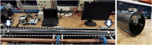
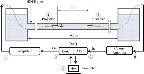
Figure 2 depicts the signal path. For the forward wave propagation, a probing signal of 3 V amplitude is defined at the computer and fed to a National Instruments (Austin, TX, USA) USB-6356 DAQ I/O board, where it is converted from the digital to the analogue domain with 16-bit accuracy. The transmission sampling rate is set to 1 MHz, adequate to resolve probing signals with a frequency content of up to 100 kHz when considering a minimum of 10 sampling points per wave period, T. A Brüel & Kjær Type 2713 Power Amplifier applies a 30 dB gain to the analogue signal (hence the output amplitude for a 3 V input signal is ∼95 V) before it is emitted from the projecting transducer. At the exact same time that transmission occurs, the sensing circuit is programmed to commence with the signal acquisition. The pulse propagates along the pipe and interacts with the boundaries before reaching the receiving transducer. The receiving hydrophone converts the mechanical movement due to pressure fluctuations into electric charge by exploiting the piezoelectric phenomenon. The charge produced as a response to mechanical stress is proportional to the pressure magnitude and the size of the piezoelectric element embedded within the hydrophone. The typical charge sensitivity of the utilized hydrophone as documented by its manufacturer is 0.1 pC Pa⁻¹, i.e. a fraction of a picoCoulomb per Pascal of applied pressure. It is, therefore, crucial to condition and amplify the signal as well as to nullify the degrading capacitance effect of the cable connecting the hydrophone to the rest of the circuit; thus, a Brüel & Kjær Type 2692-A Nexus Charge Amplifier is introduced to the signal chain. Subsequently, the analogue signal is converted to digital on the National Instruments USB-6356 DAQ I/O board, with the same resolution and sampling rate as that of the digital-to-analogue conversion. In the final step, the system response is stored in the computer. For the second part of the experiment, the roles of the transducers are interchanged: the receiver becomes the source, and the transmitted signal is the time-reversed system response recorded during the forward propagation. The pressure field generated in the waveguide by the time-reversed signal is evaluated at the location of the original source. All aspects of the signal transmission and acquisition tasks for both the forward and time reversal procedures are controlled and synchronized using a self-developed National Instruments LabVIEW code. The utilized pressure signals are Gaussian modulated sine pulses that enable the precise definition of the excited bandwidth and, hence, number of modes. More details regarding their mathematical function and characteristics are provided as supplemental online material.

Figure 2 Signal path schematic of the experimental set-up: for the forward test, the probing signal is defined at the computer (1), converted from digital-to-analogue in the DAQ board (2), amplified (3) and emitted from the projector (4). Concurrently, a receiver (5) captures the system response, the signal is conditioned (6), converted from analogue-to-digital (7), and stored in the computer (1). For the second – time-reversed – part of the test, the transducer roles are interchanged: the receiver becomes the projector and vice versa, while the emitted signal is the stored response but time-reversed (first in, last out)

2.2 Results

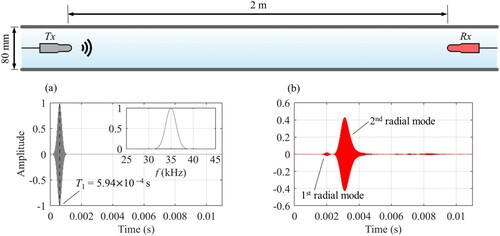
For the first trial, we probe the DN80 HDPE pipe set-up with a Gaussian modulated sine pulse of central frequency f_c = 35 kHz and 20% relative bandwidth (b = 0.2), peaking at time T₁. The wavelength associated with the central frequency of the pulse is about 4 cm, and the total duration of the signal is 5 × 10⁻³ s, accounting to 5000 samples at 1 MHz sampling rate. Figure 3 shows the results of the forward wave propagation. Specifically, Fig. 3a depicts the waveform of the pulse emanating from the projector, as evaluated by a receiver in contact with the source in initial testing, and Fig. 3b shows the acquired system response. Both waveforms presented in Fig. 3 are normalized with respect to the source amplitude. The obtained response in Fig. 3b is characteristic of the multipath wave propagation that occurs in a bounded waveguide. Prior measurements and extensive waveguide characterization with broadband signals have indicated that in the excited frequency interval (depicted in the inset of Fig. 3a) two modes propagate in total. These two modes are discernible as individual wavepackets in Fig. 3b, with the fastest reaching the receiver at t ≈ 0.002 s. To illustrate, consider each mode as a vector/ray that stems from the acoustic source at different angles with respect to the pipe centreline. The ray with the steeper angle “bounces” off the pipe walls more often compared to the other and eventually follows a longer path to the receiver. Thus, this particular mode appears “slow” and reaches the receiver at a later time than the “fast” mode, despite the fact that the wave speed, c_f, is constant. In the literature (Del Grosso, 1971; Grigoropoulos et al., 2019; Lin & Morgan, 1956), the faster mode is identified as the 1st radial, while the trailing mode is the 2nd radial; absent is the plane-like wave mode that is expected in typical water hammer. As noted in Louati and Ghidaoui (2017), the size of the source relative to the pipe cross section is the deciding factor for the excitation of the plane-like wave mode. In particular, the smaller the source compared to the pipe cross section, the lesser the energy carried from the plane-like wave. For our particular case, the transducer accounts for about 0.1 the diameter of the DN80 HDPE pipe; thus, it effectively acts as a point source that fails to excite the plane-like wave mode to detectable levels.

Figure 3 (a) A Gaussian modulated pulse is emitted from the source at one end of the pipe, with its amplitude spectrum shown in the inset. (b) The response of the system 2 m away from the source is characteristic of multipath propagation and comprises of two wavepackets, with the fastest attributed to the 1st radial, and the trailing to the 2nd radial mode

Noteworthy is that the dispersion effects are more prevalent for the case of the 2nd radial mode, as revealed by the certain elongation (or “tail”) of the pertinent wavepacket in time. This is due to the relatively larger variation in the group velocity of the 2nd radial mode in the excited frequency bandwidth compared to the 1st. Signals of negligible amplitude in the range t > 0.06 s are due to reflections from the pipe/reservoir boundaries and pipe supports. Consequently, the set-up is akin to a semi-infinite waveguide problem, and reverberations from the boundaries at both ends of the pipe that would otherwise assist in the time reversal process are precluded. The total duration of the captured signal is chosen equal to T_tot,1 = 0.011 s, as longer measurements indicate no further reflections beyond that point in time.

In the selected frequency bandwidth, it is apparent from Fig. 3b that the 2nd radial mode carries more energy in comparison to the 1st. Regardless, the accumulated amplitude of the two modes is much reduced compared to that of the injected pulse (Fig. 3a). This is partially expected due to the dispersion effects and the use of a single receiving transducer that fails to capture the transmitted wave energy in its entirety. Most crucially, however, these attenuation levels could be indicative of excessive damping due the viscous properties of the waveguide. Therefore, the validity of the time reversal process under such conditions is not certain and warrants further experimental investigation.

For the time-reversal test, the system response from the forward propagation (Fig. 3b) is reversed in time (first in, last out – Fig. 4a) and emitted from the position of the original receiver. Consequently, the slow propagating mode (2nd radial) is released first, with the fast one (1st radial) following. The response of the system to the time-reversed pulse is evaluated at the position of the original source. Figure 4 presents the results, with the source signal and pertinent system response plotted in Fig. 4a and b, respectively. All waveforms are normalized to the amplitude of the original source (Fig. 3a). Surprisingly, the originally injected signal (Fig. 3a) is recreated with great veracity (Fig. 4b), indicating that multipath effects are successfully compensated. The peak amplitude of the recreated pulse occurs at t ≈ T_tot,1 – T₁, coinciding with that of the original source with a relative error of 96.1 ppm, thus demonstrating sufficient temporal compression.

Figure 4 (a) The response of the system from the forward propagation test is time reversed and reemitted from the location of the original receiver. (b) the original pulse is successfully recreated at the location of the original source, albeit with the appearance of sidelobes

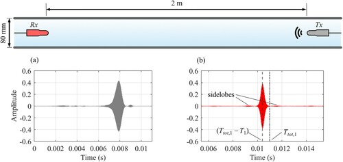
A trait of the time reversal process is the appearance of symmetric sidelobes with respect to the main pulse (indicated in Fig. 4b). Sidelobes occur due to the inability of the single transducer time reversal mirror to capture a portion of the wave energy and are suppressed if additional transducers/points are included to form a time reversal array (Roux et al., 1997). However, the experimental set-up offers limited cross-sectional space for the deployment of multiple transducers across the pipe diameter. A pipe of larger cross-sectional area and adequate accessibility options could be deployed to study the effect of multiple transducers on the focusing quality of time reversal. An alternative approach would utilize an analytical model to simulate additional transducers and study their effect to sidelobes.

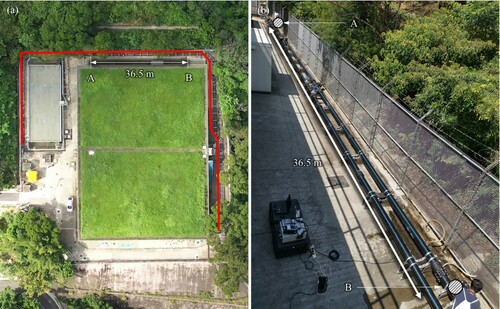
The presented results prove that time reversal of high frequency pressure waves is feasible when employed in water-filled viscoelastic HDPE pipes. The experimental set-up in the hydraulic lab of HKUST; however, features a rather small diameter pipe not found in typical water supply network installations. In addition, the distance between transducers is short and, therefore unlikely to be implemented in practice considering the scarcity of access points in such systems. Aiming to further explore time reversal in a more realistic setting, the test is repeated at a field-scale experimental facility located at Beacon Hill, Kowloon, Hong Kong. The set-up comprises a 250 m long (in total) DN150 HDPE pipe (D = 147.2 mm, h = 16.4 mm), constructed above ground and along the perimeter of the site. The pipeline is gravity-fed from the Beacon Hill freshwater reservoir, positioned about 61 m above the site level. Figure 5a depicts the outline of the complete pipeline in red. To perform the time reversal test, a straight segment along the pipe is selected, where the same transducer pair is placed x = 36.5 m apart. The distance is dictated by the access points (“A” and “B” in Fig. 5) along the pipe and corresponds to approximately 250 times the diameter (x/D = 248). In addition, since these entry points are rather confined, it is not possible to position the transducers along the pipe centreline. As a result, the generated pressure field is not axisymmetric; still, as already remarked, this has no effect on the application of time reversal. During the test, there is no flow in the pipe and ambient water pressure is held constant. The existence of water flow is not expected to significantly influence the outcome time reversal experiment given that (1) the turbulent noise is of much lower frequency than that of the injected signal, and (2) typical flow velocities are much smaller than the acoustic wave propagation speed (i.e. Mach number is small). Nonetheless, the transducer magnetic mounts could be dislocated under flow conditions, eventually changing the relative distance between the transducer set and/or their position radially. Such changes, especially during the time interval between the forward and time reversal tests, render any obtained results questionable. A flow scenario could be revisited following a redesign of the transducer mounts; as things stand, it is chosen that water remains quiescent. To purge any potential pockets of air, the system is flushed for about an hour prior to executing the test. In conclusion, this set-up provides the opportunity to test the viability of time reversal in an extreme environment which is more akin to real systems, as defined by the dimensions and the viscous characteristics of the waveguide.

Figure 5 (a), (b) The time reversal test is repeated at a field-scale facility that employs a 250 m long DN150 HDPE pipe. The transducer set is placed 36.5 m apart, as dictated by the two access points “A” and “B” along a straight segment of the set-up

For the forward test, a Gaussian modulated pulse with central frequency equal to 60 kHz and 20% relative bandwidth is selected to match the frequency response peak of the projector where the TVR = 125 dB re μPa/1 V @ 1 m, thus better exploit its capabilities. Note that the increased bandwidth results in a shorter pulse in time (Eq. 8) as compared to that implemented in the DN80 HDPE pipe set-up. In particular, the probing pulse is plotted in Fig. 6a and peaks at time T₂, while the response of the system is shown in Fig. 6b. Again, the presented waveforms in Fig. 6 are normalized by the source amplitude. The probing pulse reaches the receiver at a later time compared to the DN80 HDPE pipe set-up due to the increased range. An estimate for the wavespeed may be calculated from the arrival time of the pulse at the receiver in the order of c_f ∼ 1400 m s^–1. No reflections are observed past t ≈ 0.03 s; thus, the system is semi-infinite with regards to its boundaries. The response comprises of multiple wavepackets, each associated to an axisymmetric or asymmetric mode. Additional modes in comparison to the DN80 HDPE pipe set-up appear, since (i) the probing signal is of smaller wavelength while the lateral dimensions of the waveguide are larger, and (ii) the excited pressure field is asymmetric due to the eccentricity of the source from the pipe centre. Besides, the mode amplitudes relative to the input signal appear reduced compared to the DN80 HDPE pipe set-up, possibly due to the increased range and accumulated viscous losses. In addition, a larger portion of the propagating wave energy is unaccounted for at the receiver in comparison to the DN80 HDPE pipe set-up, given that the cross-sectional dimensions are increased while the transducer used is the same. It is, therefore, of great interest to verify time reversal in the presence of multiple modes and under the effect of the overall enhanced attenuation characteristics of the field-scale pipe.

Figure 6 The experiment is repeated for a much larger waveguide with relative dimensions x/D = 248. (a) The source signal is a Gaussian modulated pulse of central frequency f_c = 60 kHz, with its frequency content presented in the inset. (b) The system response is acquired at 36.5 m range and comprises of multiple wavepackets

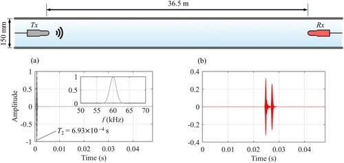
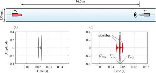
Figure 7 depicts the results of the time-reversal step, where the system response from the forward stage (Fig. 6b) is time reversed (Fig. 7a) and re-emitted from the location of the original receiver. Thereafter, the time reversed pressure field is evaluated at the position of the original source. The captured signal (Fig. 7b) reproduces the original Gaussian modulated pulse (Fig. 7a), and peaks at approximately time t ≈ T_tot,2 – T₂, with a relative error equal to 359.35 ppm. Evidently, temporal compression is not as accurate as in the DN80 HDPE pipe set-up, since the estimated time error is comparatively almost 4 times larger. Furthermore, the normalized amplitude of the recreated pulse for the case of the DN150 HDPE pipe (Fig. 7b) is smaller than that of the DN80 HDPE pipe (Fig. 4b). As already discussed, this is to be expected due to the increased range (with an accompanying increase of viscous losses) and the narrow aperture area of the time-reversal mirror (TRM). Also noteworthy is that the sidelobes of the recreated signal in Fig. 7b are far more pronounced than that in the DN80 HDPE pipe set-up (Fig. 4b), possibly because the modes contributing to the formation of the said sidelobes carry more energy (and/or are not attenuated as much). Ultimately, however, the presented experimental results prove the validity of time reversal in an adverse environment that involves (1) viscoelastic boundaries with considerable damping, (2) a single-channel time reversal mirror of limited size relative to the cross-section of the waveguide, and (3) semi-infinite boundaries.

Figure 7 (a) The response of the DN150 HDPE pipe set-up from the forward test is time-reversed and emitted from the location of the original receiver. (b) The original pulse is recreated at the location of the original source and time t ≈ T_tot,2 – T₂ displaying sufficient temporal compression

2.3 Spatial focusing

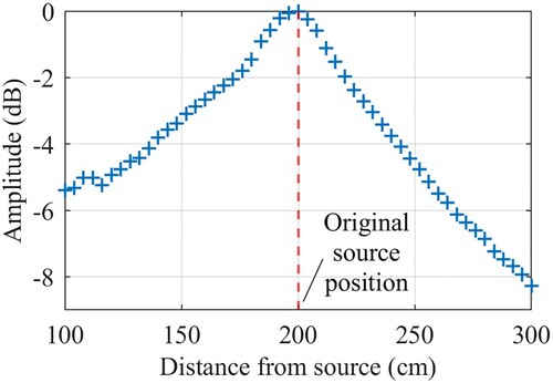
The experimental results introduced so far merely demonstrate the time compression properties of the time reversal process. It is also important to validate that the time reversed signal refocuses only at the location of the initial source. This time reversal attribute is particularly important for pulse-echo detection methods where the objective is to uniquely identify a target, e.g. a pipe leak or blockage. Here, spatial focusing is tested experimentally in the DN80 HDPE pipe set-up by performing several measurements at wavelength multiples along the pipe length, where x ∈ [1,3] m. To intensify the effects of dispersion in the limited available range of the set-up, a signal of wider bandwidth than the previous tests is chosen where f_c = 35 kHz and b = 0.6. By doing so, the 2nd radial mode “spreads” more in time compared to the response observed in Fig. 3b and time compression at the location of the original source is emphasized. In particular, we first perform the forward test, placing the transducer pair at 2 m distance. Then, the transducer roles are interchanged but instead of keeping the distance fixed at 2m, the time reversal receiver is moved longitudinally along the pipe. Figure 8 presents a selection of three measurements at 1, 2 and 3 m away from the time reversal source. It is evident that the time reversed pressure field is time compressed and maximized only at the location of the original source, i.e. 2 m away from the source.

Figure 8 The time reversed pressure field is evaluated at multiple locations along the pipe. Here, the waveform at three locations is presented: 2 m (in blue), 1 m (in orange), and 3 m (in yellow) away from the time reversal source. The signal compresses and obtains its maximum amplitude 2 m from the time reversed source, coinciding with the location of the original source

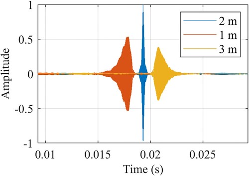
Figure 9 presents the maximum amplitude of the time reversed response at additional locations. Still, the peak of the plot is observed 2 m away from the time reversal source, coinciding with the location of the original source, thus verifying the spatial focusing properties of the time reversed pressure field. It should be noted that measurement intervals smaller than λ do not yield substantial differences due to the diffraction limit. Similar results were demonstrated in Roux et al. (1997) for a bounded waveguide. However, unlike Roux et al. (1997), herein: (1) the boundaries are viscoelastic instead of steel, thus manifesting damping; (2) the relative dimensions of the current waveguide are significantly larger; and (3) a single-channel time reversal mirror is used. In the next section, we try to gain some insight into the reasons time reversal is successful in the presented experiments despite the presence of viscous damping in both the fluid and pipe wall.

Figure 9 Multiple measurements are performed along the DN80 HDPE pipe at wavelength multiples to demonstrate spatial focusing. Maximum amplitude for the time reversed pressure field is observed at the location of the original source

3 Time reversal invariance in a viscous waveguide through scaling analysis

Wave propagation is robust to time reversal, but particle motion is not (Snieder & Scales, 1998). In fact, it is the irreversibility of particle motion that prevents, say, a broken egg from becoming whole again by reversing the velocity of its shattered pieces. Waves, on the other hand, are found to be time reversible as exemplified by the experiments of our own and others (to be discussed in following sections of this manuscript). Therefore, when contemplating time reversal, it is important to distinguish whether the process one intends to reverse relies on particle motion or wave propagation. It is the impression of the authors that time reversal is often dismissed altogether because it is thought in the context of particles and not waves.

Why is the motion of particles not time reversible, but the propagation of waves is? The two mechanisms that limit or even prevent time reversibility are damping and stability (Snieder, 2002). To understand the effect of damping on limiting the time reversibility of particle motion, consider a mass m in free fall. The forces on this particle are gravity and air resistance. Solving for the particle position z as a function of time gives: (3) $z\left(t\right)=\frac{m^{2}g}{\eta }\left[1+\frac{\eta t}{m}-e^{\frac{\eta t}{m}}\right]=-\frac{1}{2}g{t}^2-\frac{\eta t^3}{m}\frac{g}{3!}+\dots$(3) where η is a parameter that characterizes air resistance, and g is the acceleration of gravity. Applying the transformation t → −t gives: (4) $z\left(-t\right)=\frac{m^{2}g}{\eta }\left[1-\frac{\eta t}{m}-e^{\frac{-\eta t}{m}}\right]=-\frac{1}{2}g{t}^2+\frac{\eta t^3}{m}\frac{g}{3!}+\dots$(4) Although z(t) ≠ z(−t), it is clear that the difference between the forward and time reversed paths is negligible when (ηt³g/6 m)/(gt²/2) ≪ 1. That is, in the presence of friction, time reversibility approximately holds if: (5) $TR=\frac{\eta t}{3m}\ll 1$(5) where TR is a time reversibility parameter. Equation (5) points out the important fact that the relative effect of damping grows linearly in time (∝ t). That is, a particle loses its ability to retrace its forward path with time in a linear manner. The elapsed time t for which time-reversibility is expected to be lost is ηt/3 m ∼ 1 or larger, which leads to t ∼ 3 m/η or larger. We will show later in the manuscript that an analogous expression to Eq. (5) arises when we study the time reversibility of the Navier–Stokes and the viscoelastic pipe wall equations.

Now the effect of instability on the time reversal of particle motion is introduced. Consider a cloud of interacting particles. At time t = T_tot, the position x_i(T_tot) and velocity v_i(T_tot) of each particle i is recorded and the particles are captured. What is the path of the captured particles if each is released with initial velocity equal to − v_i(T_tot) (i.e. velocity is time reversed) plus a small perturbation? Snieder (2002) showed that the perturbed system is unstable in the sense that the path traced by the particles in the reversed stage diverges exponentially in time from the path traced in the forward stage (i.e. exp(βt), where β is parameter that depends on length scale and particle density). Note that the contribution of instabilities grows exponentially in time, while that of damping only linearly. Therefore, it is this instability that prevents the time reversibility of particles.

Regarding the time reversibility of the waves, Snieder and Scales (1998) proved theoretically and numerically that waves are far more stable than particles to time reversal. Consider n scatterers situated between the wave source and receiver. The time reversed (phase conjugated) pressure field has the following form: (6) $\begin{array}{rl}{p}_{tr}\left(\mathit{r}\right)& \sim \frac{\sin k_{max}\left[|{\mathit{r}}_{\mathit{R}}-{\mathit{r}}_{\mathit{S}}|-|\mathit{r}-{\mathit{r}}_{\mathit{R}}|\right]}{|{\mathit{r}}_{\mathit{R}}-{\mathit{r}}_{\mathit{S}}|-|\mathit{r}-{\mathit{r}}_{\mathit{R}}|}\\ & +\sum _{i=1}^n{\alpha }_i\frac{\begin{array}{c}\sin k_{max}[|{\mathit{r}}_{\mathit{R}}-{\mathit{r}}_{\mathit{i}}|+|{\mathit{r}}_{\mathit{i}}-{\mathit{r}}_{\mathit{S}}|\\ -|{\mathit{r}}_{\mathit{R}}-{{\mathit{r}}^{\mathbf{\prime }}}_{\mathit{i}}|-|{{\mathit{r}}^{\mathbf{\prime }}}_{\mathit{i}}-\mathit{r}|]\end{array}}{|{\mathit{r}}_{\mathit{R}}-{\mathit{r}}_{\mathit{i}}|+|{\mathit{r}}_{\mathit{i}}-{\mathit{r}}_{\mathit{S}}|-|{\mathit{r}}_{\mathit{R}}-{{\mathit{r}}^{\mathbf{\prime }}}_{\mathit{i}}|-|{{\mathit{r}}^{\mathbf{\prime }}}_{\mathit{i}}-\mathit{r}|}\end{array}$(6) where p_tr is the time reversal pressure field value, α_i is a measure of the scattering strength of scatterer i, r_i and r_i′ are the unperturbed and perturbed locations of the ith scatterer, r_S and r_R are the locations of the source and receiver during the forward propagation stage, while r is the receiver location during the time reversal stage. Moreover, k_max is the wavelength associated with the largest frequency in the bandwidth of the probing signal. Equation (6) describes the time reversed pressure field as a superposition of the unperturbed wave that follows a direct path from the time reversal source at r_R to the measurement location r, and the scattered waves that track an indirect path from r_R to the scatterer locations r_i and then to r. The former path is expressed in the first term, while the latter in the second term on the right-hand side of Eq. (6). Let r_i′ − r_i = e_i be the perturbation of the location of the ith scatterer. Using the fact that sinx/x → 1 as x → 0, the time reversed wave refocuses at the source r_S when r = r_S (i.e. at the original source location), and e_i = 0. What is the effect to time reversal when the scatterers are perturbed form their forward propagation positions? We now consider the time reversal field at r = r_S when e_i is a random perturbation. Taylor’s series expansion leads to: (7) $p_{tr}\left(\mathit{r}={\mathit{r}}_{\mathit{S}}\right)\sim 1-\frac{1}{3!}\sum _{i=1}^n{\alpha }_i{k}_{max}^2{|{\mathit{e}}_{\mathit{i}}|}^2$(7) The rate of degradation of time reversal due to a perturbation error |e_i| is: (8) $\frac{\mathrm{\partial }{p}_{tr}}{\mathrm{\partial }|{\mathit{e}}_{\mathit{i}}|}\sim \frac{{\alpha }_i}{3}{k}_{max}^2|{\mathit{e}}_{\mathit{i}}|$(8) The standard deviation of the refocusing degradation is: (9) ${\left[\sum _{i=1}^{n}E\left[{\left(\frac{\mathrm{\partial }{p}_{tr}}{\mathrm{\partial }|{\mathit{e}}_{\mathit{i}}|}\right)}^2\right]\right]}^{0.5}\sim \frac{\sqrt{n}}{\sqrt{3}}{k}_{max}{\sigma }_0\sqrt{\sum {\alpha }_i^2}$(9) The number of scatterers a wave meets during time t is (Snieder & Scales, 1998): (10) $n\sim \frac{ct}{d}$(10) where c is the wave speed and d is the average distance between scatterers. As a result, the degradation of the wave refocusing is given by the following dimensionless standard deviation: (11) ${\sigma }_{tr}\left(t\right)=\sqrt{\sum _{i=1}^n{\alpha }_i^2}\frac{2\pi f_{max}}{c}{\sigma }_0\sqrt{\frac{ct}{d}}$(11) which shows that the degradation of the quality of the time reversal refocusing grows as (t^1/2). This result concurs with the theoretical and experimental findings of Snieder and Scales (1998). The following statement from Snieder (2002, p. 14) succinctly contrasts the time reversibility of particle and waves vis-à-vis instabilities:

Physically there are two reasons that explain this difference [between time reversibility of particles and waves]. The particles are point-like objects with no scale, whereas the waves are associated with a wavelength. The wave field “feels” its environment on a scale that only depends on the wavelength; hence the wavelength determines a natural scale for the sensitivity of scattered waves for perturbations of the scatterer locations. In addition, the waves travel along all possible scattering paths, whereas the particles each travel along a unique path. When the scatterer locations are perturbed, the waves still travel along all possible scattering paths, whereas a particle may suddenly follow a fundamentally different trajectory.

We proceed to investigate the effect of damping on the time reversibility of waves, where the pertinent viscous equations of motion for the waveguide are now considered. The point form of the momentum conservation equation for the fluid is: (12) $\begin{array}{rl}& {\rho }_f\left(t\right)\frac{{\text{d}}^{\text{2}}\mathit{r}\left(t\right)}{\text{d}{t}^2}+{\rho }_f\left(t\right)\frac{\text{d}\mathit{r}\left(t\right)}{\text{d}t}\\ & \cdot \mathrm{\nabla }\frac{\text{d}\mathit{r}\left(t\right)}{\text{d}t}+\mathrm{\nabla }p\left(t\right)-\mathrm{\nabla }\cdot \tau \left(t\right)+{\rho }_f\left(t\right)\mathit{g}=0\end{array}$(12) where τ is the viscous stress tensor, p is the fluid pressure, and g is the acceleration of gravity. Note that for clarity and ease of presentation of the time reversal concept we follow the tradition of writing the equation in terms of position r(t), and not velocity v(t). Also, 0 corresponds to a zero vector. The general expression of the viscous stress forces ∇·τ for a compressible Newtonian fluid is: (13) $\begin{array}{rl}\mathrm{\nabla }\cdot \tau \left(t\right)& =\mu \left\{{\mathrm{\nabla }}^{\text{2}}\frac{\text{d}\mathit{r}\left(t\right)}{\text{d}t}+\frac{1}{3}\mathrm{\nabla }\left[\mathrm{\nabla }\cdot \frac{\text{d}\mathit{r}\left(t\right)}{\text{d}t}\right]\right\}\\ & +\kappa \left\{\mathrm{\nabla }\left[\mathrm{\nabla }\cdot \frac{\text{d}\mathit{r}\left(t\right)}{\text{d}t}\right]\right\}\end{array}$(13) where μ, κ are the dynamic and bulk fluid viscosities, respectively. As regards to the pipe wall viscous equations, we restrict our argument to the radial momentum component for brevity: (14) $\begin{array}{rl}& {\rho }_p\left(t\right)h\frac{{\mathrm{\partial }}^{2}w\left(t\right)}{\mathrm{\partial }{t}^2}\\ & =\frac{\mathrm{\partial }S\left(t\right)}{\mathrm{\partial }x}-\frac{1}{J\left(t\right)}\frac{h}{\left(1-{\nu }_p^2\right)}\left(\frac{w\left(t\right)}{R^2}+\frac{v_p}{R}\frac{\mathrm{\partial }u\left(t\right)}{\mathrm{\partial }x}\right)+p\left(t\right)\end{array}$(14) where w, u are the radial (r) and axial (x) displacements of the centroid of a pipe wall element, respectively, R is the pipe radius, ρ_p is the density, and ν_p is Poisson’s ratio of the pipe wall material. Note that the fluid pressure p(t) at the pipe/fluid interface is inserted in Eq. (14) as forcing to the pipe wall. In addition, S(t) represents the shear forces developing in the pipe wall per unit length, given by: (15) $S\left(t\right)=\frac{Kh}{2J\left(t\right)\left(1+v_p\right)}\left[\frac{\mathrm{\partial }w\left(t\right)}{\mathrm{\partial }x}-\alpha \left(t\right)\right]$(15) where K is a correction factor for the distribution of the shear forces across the pipe thickness, and α is the angular rotation of a radial line about an axis that crosses the pipe wall element centroid and is normal to the x–r plane (x is along the length of the pipe, and r along the pipe radius). Finally, J(t) corresponds to the time dependent creep compliance, assumed to follow the generalized Kelvin–Voigt (GKV) model. Accordingly: (16) $J\left(t\right)=J_0+\sum _{j=1}^{N_{kv}}{J}_j\left[1-exp\left(\frac{-t}{{\tau }_j}\right)\right]$(16) where N_kv is the number of GKV elements, each described by a creep coefficient J_j and relaxation time τ_j. For the interested reader, the full set of equations of motion for the pipe wall, as well as the time reversal transformation for the inviscid waveguide equations, are provided as supplemental online material.

Now, the time reversal transformation t → −t for the viscous fluid momentum conservation equation (Eq. 12) is: (17) $\begin{array}{rl}& {\rho }_f\left(-t\right)\frac{{\text{d}}^{\text{2}}\mathit{r}\left(-t\right)}{\text{d}{\left(-t\right)}^2}+{\rho }_f\left(-t\right)\frac{\text{d}\mathit{r}\left(-t\right)}{\text{d}\left(-t\right)}\\ & \cdot \mathrm{\nabla }\frac{\text{d}\mathit{r}\left(-t\right)}{\text{d}\left(-t\right)}+\mathrm{\nabla }p\left(-t\right)-\mathrm{\nabla }\cdot \tau \left(-t\right)+{\rho }_f\left(-t\right)\mathit{g}=0\end{array}$(17) Considering d²·/d(−t)² = d²·/dt², and d·/d(−t) = −d·/dt, Eq. (17) becomes: (18) $\begin{array}{rl}& {\rho }_f\left(-t\right)\frac{{\text{d}}^{\text{2}}\mathit{r}\left(-t\right)}{\text{d}{t}^2}+{\rho }_f\left(-t\right)\frac{\text{d}\mathit{r}\left(-t\right)}{\text{d}t}\\ & \cdot \mathrm{\nabla }\frac{\text{d}\mathit{r}\left(-t\right)}{\text{d}t}+\mathrm{\nabla }p\left(-t\right)-\mathrm{\nabla }\cdot \tau \left(-t\right)+{\rho }_f\left(-t\right)\mathit{g}=0\end{array}$(18) It is interesting to note that the nonlinear operator term in Eq. (18) which is responsible for the fluid turbulence retains its form; thus, it is time reversible. This fact has also been experimentally demonstrated in Chaiken et al. (1986) where the mixing between two fluids of different colours was undone by performing the opposite, time reversed, motion. On the other hand, the form of the viscous term in the time reversal stage is: (19) $\begin{array}{rl}\mathrm{\nabla }\cdot \tau \left(-t\right)& =\mu \left\{{\mathrm{\nabla }}^{\text{2}}\frac{\text{d}\mathit{r}\left(-t\right)}{\text{d}\left(-t\right)}+\frac{1}{3}\mathrm{\nabla }\left[\mathrm{\nabla }\cdot \frac{\text{d}\mathit{r}\left(-t\right)}{\text{d}\left(-t\right)}\right]\right\}\\ & +\kappa \left\{\mathrm{\nabla }\left[\mathrm{\nabla }\cdot \frac{\text{d}\mathit{r}\left(-t\right)}{\text{d}\left(-t\right)}\right]\right\}\\ & =-\mu \left\{{\mathrm{\nabla }}^{\text{2}}\frac{\text{d}\mathit{r}\left(-t\right)}{\text{d}t}+\frac{1}{3}\mathrm{\nabla }\left[\mathrm{\nabla }\cdot \frac{\text{d}\mathit{r}\left(-t\right)}{\text{d}t}\right]\right\}\\ & -\kappa \left\{\mathrm{\nabla }\left[\mathrm{\nabla }\cdot \frac{\text{d}\mathit{r}\left(-t\right)}{\text{d}t}\right]\right\}=-\mathrm{\nabla }\cdot \tau (-t\end{array}$(19) Combining Eqs (18) and (19) gives: (20) $\begin{array}{rl}& {\rho }_f\left(-t\right)\frac{{\text{d}}^{\text{2}}\mathit{r}\left(-t\right)}{\text{d}{t}^2}+{\rho }_f\left(-t\right)\frac{\text{d}\mathit{r}\left(-t\right)}{\text{d}t}\\ & \cdot \mathrm{\nabla }\frac{\text{d}\mathit{r}\left(-t\right)}{\text{d}t}+\mathrm{\nabla }p\left(-t\right)+\mathrm{\nabla }\cdot \tau \left(-t\right)+{\rho }_f\left(-t\right)\mathit{g}=0\end{array}$(20) which differs in form from Eq. (12) due to the change in sign of the viscous term, ∇ · τ(t). Thus, the viscous fluid flow equations are not time reversible.

The momentum equation along the radial coordinate for a viscous pipe wall element under time reversal transformation (t → −t) becomes: (21) $\begin{array}{rl}& {\rho }_p\left(-t\right)h\frac{{\mathrm{\partial }}^{2}w\left(-t\right)}{\mathrm{\partial }{\left(-t\right)}^2}\\ & =\frac{\mathrm{\partial }S\left(-t\right)}{\mathrm{\partial }x}-\frac{1}{J\left(-t\right)}\frac{h}{\left(1-{\nu }_p^2\right)}\left(\frac{w\left(-t\right)}{R^2}+\frac{v_p}{R}\frac{\mathrm{\partial }u\left(-t\right)}{\mathrm{\partial }x}\right)\\ & +p\left(-t\right)\end{array}$(21) with (22) $S\left(-t\right)=\frac{Kh}{2J\left(-t\right)\left(1+v_p\right)}\left[\frac{\mathrm{\partial }w\left(-t\right)}{\mathrm{\partial }x}-\alpha \left(-t\right)\right]$(22) Since ∂²·/∂ (−t)² = ∂²·/∂t², Eq. (21) becomes: (23) $\begin{array}{rl}& {\rho }_p\left(-t\right)h\frac{{\mathrm{\partial }}^{2}w\left(-t\right)}{\mathrm{\partial }{t}^2}\\ & =\frac{\mathrm{\partial }S\left(-t\right)}{\mathrm{\partial }x}-\frac{1}{J\left(-t\right)}\frac{h}{\left(1-{\nu }_p^2\right)}\left(\frac{w\left(-t\right)}{R^2}+\frac{v_p}{R}\frac{\mathrm{\partial }u\left(-t\right)}{\mathrm{\partial }x}\right)\\ & +p\left(-t\right)\end{array}$(23) First, p(−t) ≠ p(t) since the viscous flow equations are not time reversible as can be seen by comparing Eq. (12) and Eq. (20). In addition, the creep function J(t) (Eq. 16) under time reversal is expressed as: (24) $J\left(-t\right)=J_0+\sum _{j=1}^{N_{kv}}{J}_j\left[1-\exp \left(\frac{t}{{\tau }_j}\right)\right]$(24) Hence, the exponential decay in Eq. (16) gives way to an exponential growth in Eq. (24) and, as such, J(−t) ≠ J(t). Consequently, the differential operator that governs r(t), u(t), w(t), α(t), ρ_f(t), ρ_p(t), S(t) and p(t) is dissimilar to that which governs r(−t), u(−t), w(−t), α(−t), ρ_f(−t), ρ_p(−t), S(−t) and p(−t). This breakdown of time reversal is due to the viscous terms appearing in both the fluid and pipe wall equations. Nonetheless, the experiments presented in the preceding section demonstrate that acoustic waves propagating in water filled viscoelastic pipes are time reversible over a frequency bandwidth ranging from 24.5 to 66 kHz. In addition, time reversal has been verified in the lab and field in many systems where damping is present (e.g. gravity waves and acoustic waves in the ocean which are discussed later in the manuscript). How can this apparent contradiction between theory and experiment be reconciled?

A plausible explanation requires that the viscous terms in the governing equations be much smaller than the pertinent temporal acceleration terms. To investigate this hypothesis, we perform a scale analysis for both viscous fluid and pipe wall equations of motion. Consider a disturbance in the fluid medium that generates a propagating wave of length scale λ. Commencing with the fluid domain, the ratio of the viscous forces term to the temporal acceleration term, i.e. the inverse Reynolds number 1/R_e is: (25) $T{R}_f=\frac{\mathrm{\nabla }\cdot \tau }{{\rho }_f\left(t\right)\frac{\mathrm{\partial }\mathit{v}\left(t\right)}{\mathrm{\partial }t}}\sim \frac{\nu \frac{||\mathit{v}||}{{\lambda }^2}}{\frac{||\mathit{v}||}{t}}=\nu \frac{t}{{\lambda }^2}\approx \frac{1}{{\mathsf{R}}_{\mathsf{e}}}\frac{t}{T}=\frac{ft}{{\mathsf{R}}_{\mathsf{e}}}$(25) where ν (= μ/ρ_f) is the kinematic viscosity, T = λ/c_f, t/T represents the dimensionless elapsed time from the moment the wave disturbance is introduced, and c_f is the wave speed in the fluid. Equation (25) defines the time reversibility parameter of waves in the fluid domain. Note the fact, well-known since the mid-nineteenth century, that viscous effects grow with frequency (Stokes, 2009) is evident in Eq. (25).

For the case of the pipe wall, there are in total three components of the momentum equation. A complete scale analysis is given in the online supplemental material, Chapter S.3; here, the discussion is limited to the most unfavourable scenario (i.e. the component of the momentum equation with dominant viscosity). This case is recovered from the radial momentum component (Eq. S.10) when the ratio of the viscous radial component of the hoop stresses to the pertinent inertial term is considered. The ratio of damping to inertia over time t in the pipe wall obtained from Eq. (S.10) is: (26) $\frac{\sum _{j=1}^{N_{kv}}\frac{J_j}{J_0^2}\left(\frac{t}{{\tau }_j}\right)\frac{h}{\left(1-{\nu }_p^2\right)}\frac{w\left(t\right)}{R^2}}{{\rho }_p\left(t\right)h\frac{{\mathrm{\partial }}^{2}w\left(t\right)}{\mathrm{\partial }{t}^2}}\sim \frac{t}{t_v{J}_0{f}^2{R}^2{\rho }_p\left(1-{\nu }_p^2\right)}=T{R}_p$(26) Equation (26) defines the time reversibility parameter of waves propagating in the pipe wall, TR_p. Moreover, Eq. (26) introduces the pipe viscous time scale t_v, that is retrieved from the GKV model expression and corresponds to the time scale viscous effects in the pipe wall become significant (Eq. S.18 of the online supplemental material). Unlike Eq. (25), Eq. (26) shows that the viscous damping from the pipe wall diminishes at high frequencies. This is due to the fact that pipe viscous damping is only significant when the time scale of the wave is of the same order of magnitude to the time scale of the viscous damping and reduces quickly when these time scales become different (Serra-Aguila et al., 2019).

The relative order of magnitude of the viscous force to temporal acceleration terms for the combined fluid-pipe wall system involves adding Eq. (25) to (26) and the result is: (27) $t\frac{\nu f^2}{c_f^2}+\frac{t}{t_v{J}_0{f}^2{R}^2{\rho }_p\left(1-{\nu }_p^2\right)}=TR$(27) where TR is the time reversibility parameter for the whole system (i.e. fluid and pipe wall). It is chosen to add the viscous effect from the two domains instead of taking the maximum, since the former is a more unfavourable scenario. Equation (27) shows that the contribution of damping towards the time irreversibility of waves in a viscoelastic pipeline grows linearly with time t. In contrast, the contribution of the instability to the wave propagation and, thus, its time irreversibility grows only as (t^1/2) (Snieder, 2002). Note that the time scale here is defined as the ratio of the elapsed time from the initiation of the disturbance over the wave period, and for high frequency waves, t/T >> 1. Therefore, the reversibility (or irreversibility) of waves is governed by damping. The ratio of the viscous to temporal acceleration terms can also be written in terms of wave energy ratio as follows: (28) $TR\sim \ln \frac{E_a\left(t\right)}{E_{a,0}}\sim \ln \frac{p^2\left(t\right)}{p_0^2}$(28) where E_a,0 is the energy of the wave at the source, and E_a(t) is the energy of the wave after it has propagated over time t. The scaling can be extended to pressure amplitudes, since E_a ∝ p².

4 Discussion of the time reversal experiments

We now discuss our time reversal experiments in light of the time reversal parameter, TR. We consider an elapsed time t = x/c, where x is the distance between the transducer set in the DN150 HDPE pipe set-up (x = 36.5 m). From Fig. 6b we obtain t ∼ 2.5 × 10⁻³ s; thus, the wavespeed c_f ∼ 1.5 × 10³ m s⁻¹. According to the experiments presented in Section 2, the probing wave frequency f ∼ 10⁵ Hz. Since there is no flow, it is not necessary to use a turbulent viscosity value; thus, we apply the kinematic water viscosity ν ∼ 10⁻⁶ m² s⁻¹. The viscoelastic parameters of the GKV elements, J_j and τ_j, are adopted from Wang et al. (2019) who experimentally calibrated these parameters for three GKV elements (j = 3) based on a set-up that employs an identical HDPE pipe to the one presented in our experiments. Thus, we employ the same values (Table S.1) to obtain t_v ∼ 10⁻¹ s. The remaining pipe mechanical parameters are given in Table 1. Substituting these values in Eq. (25) yields TR_f = 10⁻⁵, while Eq. (26) returns TR_p =10⁻².

The combined effect of pipe and fluid viscosity given by Eq. (27) is TR = 10⁻² + 10⁻⁵ ≅ 10⁻²; thus, revealing that even in the wider range of our DN150 HDPE pipe set-up, the temporal acceleration terms are still some orders of magnitude larger than the pertinent viscous terms in both the fluid and HDPE pipe wall domains. Note that the viscous losses in the HDPE pipe are comparatively more significant than the viscous losses in the water, as demonstrated by the three-order difference between TR_p = 10⁻² and TR_f = 10⁻⁵.

Now that we confirmed that viscous effects are small in the range x of the experiments prescribed in this manuscript, a natural question is: what is the range x = ct where viscous terms become significant so that time reversal breaks down? At said range, the viscous terms are comparable to the temporal acceleration terms (i.e. TR ∼ 1). Setting the right-hand side of Eq. (27) to 1 and solving for x gives: (29) $x=\frac{c_f^3{c}_p{t}_v{J}_0{f}^2{R}^2{\rho }_p(1-{\nu }_p^2)}{\nu f^4{c}_p{t}_v{J}_0{R}^2{\rho }_p(1-{\nu }_p^2)+c_f^3}$(29) The pertinent parameter values from the experimental set-ups are substituted in Eq. (29), and the estimated achievable range x ∼ 110 m. Therefore, from Eq. (28) we may estimate that pipe wall viscosity in our experiment reduces the energy of the wave by about 60% every 110 m. This distance, being three times 36.5 m (i.e. the distance between the projector and receiver in our experiment), further supports the experimental findings that high-frequency waves (f ∼ 10⁵ Hz) are time reversible.

As mentioned previously, the water in the experimental set-ups is quiescent. In practice, however, water supply flows are generally turbulent. To take this situation into account, the eddy viscosity ν_t is used instead of the kinematic viscosity ν in estimating the time reversal parameter. Experimental measurements on fully developed turbulent flows in pipes (Laufer, 1953) indicate a dimensionless eddy viscosity ν_t/(V*R) of at most 0.08. In the expression of the dimensionless eddy viscosity, V* is the friction velocity defined as V* = V̄ (f_DW/8)^1/2 with V̄ being the cross-sectional average flow velocity, and f_DW is the Darcy friction factor. Assuming a typical roughness factor for the DN150 HDPE pipe k = 1.5 × 10⁻⁶ m and an extreme case for the cross-sectional average flow velocity V̄ = 3 m s⁻¹, we use the Colebrook–White equation to estimate f_DW = 0.0136. The end result is V* = 0.12 m s⁻¹ and ν_t = 1.45 × 10⁻³ m² s⁻¹. The calculated eddy viscosity is several orders of magnitude larger than the kinematic viscosity v already considered. The combined effect of turbulence and pipe wall viscosities reduces the energy of the wave by about 60% every 80 m when the frequency of the wave source is ∼ 10⁵ Hz. That is, the turbulence damping reduces the range from 110 m to 80 m (i.e. 30 m range reduction).

The range calculated in Eq. (29) for our experimental set-up is dominated by the viscous losses in the pipe wall. However, if the pipe walls were elastic, the achievable range would only be limited by the flow viscosity, resulting in x ∼ 33 km (using the fluid viscosity ν for quiescent water). In particular, the experiments we conducted test time reversibility under the most extreme condition. That is, proving that waves in HDPE pipes are time reversible guarantees that such waves are also time reversible over a wide range of other pipe materials, such as ductile iron, steel and concrete.

The presented analysis confirms that the viscous terms in both the fluid and pipe wall equations of motion are small when compared to the appropriate temporal acceleration terms, when considering the characteristic scales of our experimental set-ups. Thus, we show that contrary to the apparent invalidity of the equations of motion when t → − t due to the presence of the viscous terms, time reversal is practically feasible provided that the dimensionless parameter TR << 1. Moreover, the TR parameter can be applied on a plethora of environments to estimate the effect of viscosity to wave propagation. To our knowledge, the presented work is the first-ever direct proof of the time reversibility of pressure waves in viscoelastic pipes. As noted in (Kuperman, 2016):

An interesting take on time reversal is that when time reversal works, it can be thought of as a kind of proof of existence that the medium supports the localization goal of beamforming (BF) and/or matched field processing (MFP).

The developed scales have important practical implications. For example, to achieve a successful defect detection in pipelines using the MFP method, it is recognized that a signal-to-noise ratio (SNR) at least equal to −5 dB is necessary (Wang & Ghidaoui, 2018). Knowledge of the minimum SNR for defect detection in a particular system allows the analyst to determine the required strength of the probing signal for a desired range x. Alternatively, given the power of the source, the maximum range for successful defect detection can be estimated. For this purpose, the derived scale of viscous over the inertial forces can be applied. We rewrite Eq. (28) and set t = x/c to obtain: (30) $x\left[\frac{\nu f^2}{c_f^2}+\frac{1}{c_p{t}_v{J}_0{f}^2{R}^2{\rho }_p\left(1-{\nu }_p^2\right)}\right]=C\ln \frac{E_a\left(x\right)}{E_{a,0}}\sim C\ln \frac{p^2\left(x\right)}{p_0^2}$(30) where C is a proportionality factor that could be estimated from experimental results. The right-hand side of Eq. (30) may be expressed in terms of SNR as: (31) $C\ln \frac{p^2\left(x\right)/n^2}{p_0^2/n^2}=C\frac{\ln \left(10\right)}{10}\left[\text{SNR}\left(x\right)-\text{SNR}\left(0\right)\right]$(31) where n corresponds to the system noise, and SNR(x) = 10log₁₀(p²(x)/n²). Thus, the relationship between the SNR at the source, range x, and the desired SNR at x is written as: (32) $x=\frac{C\ln \left(10\right)}{10\left[\frac{{\nu }_t{f}^3}{c_f^2}+\frac{1}{c_p{t}_v{J}_0{f}^2{R}^2{\rho }_p\left(1-{\nu }_p^2\right)}\right]}\left[\text{SNR}\left(x\right)-\text{SNR}\left(0\right)\right]$(32) As an example, we use pressure measurements from two different locations x₁ and x₂ along the DN80 HDPE pipe (Section 2.3) to establish C ∼ −0.013. For the source levels used in this set-up, SNR(0) ∼ 31 dB. Thus, if we target a SNR(x) = −5 dB (i.e. the minimum required for defect detection using long waves), the range x ∼ 12 m. The measurements and calculations are repeated for the DN150 pipe set-up to retrieve a proportionality factor C ∼ −0.02 and SNR(0) ∼ 24 dB. For a SNR(x) = −5 dB, the estimated range is x ∼ 170 m. In Section 2.3, experimental results from multiple measurements along the DN80 HDPE pipe show an effective attenuation for the propagating modes in the frequency bandwidth of about 3 dB m⁻¹. In contrast, similar measurements in the DN150 HDPE pipe set-up show an effective attenuation of about 0.2 dB m⁻¹. The reader is reminded that the excited frequency bandwidth in the latter pipe set-up is higher (about double) than in the former. Equation (26) reveals that viscous forces in the pipe wall are inversely proportional to the probing frequency f. Also remarkable is the fact that pipe radius R appears in the denominator of Eq. (26), denoting that viscous losses are decreased for the case of the larger pipe. Therefore, the reduced attenuation in the DN150 HDPE pipe (in comparison to the DN80 HDPE pipe) could be attributed to both the higher frequency f of the probing signal, as well as the increased pipe radius R. Note that if the target SNR(x) is increased (for a given source strength), the estimated range x is reduced.

Equation (32) is also applicable to hydraulic systems where the conduits are elastic by simply omitting the second term in the denominator that accounts for the viscous pipe damping: (33) $x=\frac{C\ln \left(10\right)}{10\left(\frac{{\nu }_t{f}^2}{c_f^3}\right)}\left[\text{SNR}\left(x\right)-\text{SNR}\left(0\right)\right]$(33) Equation (33) shows that the range of waves in elastic pipes is inversely proportional to probing frequency f. For this reason, low frequency pressure transients have been successfully employed in pipeline defect detection over long distances. For example, Meniconi et al. (2018) performed low-frequency (f ∼ 10 Hz) transient tests by pump shutdown in a real 1322 m steel transmission line in Trento, Italy to identify a simulated leak. The authors reported that the transmission line was a steel DN500 pipe, with V̄ = 0.2 m s⁻¹, and estimated roughness k = 8 × 10⁻⁴ m. Hence, an applicable eddy viscosity is estimated in the order of ν_t ∼ 10⁻⁴ m² s⁻¹. Author-provided data from initial transient tests on the intact system indicate a SNR(0) ∼ 51 dB at the source and are used to obtain a proportionality factor C = −3.1 × 10⁻³. Now, assuming a range x equal to the overall transmission pipe length (x = 1322 m), Eq. (33) estimates the SNR(x) ∼ 51 dB. The calculated SNR(x) is much larger than the minimum of –5 dB required for defect detection in pipes, which supports the findings of Meniconi et al. (2018) and proves that low-frequency waves have a very long range in an elastic transmission line. In Meniconi et al. (2015), similar tests were conducted along an even longer 6301.4 m water supply pipe in the city of Milan, Italy. According to the authors, the largest part of the pipeline comprised of a steel DN800 pipe, and the system was rated for a maximum cross-sectional average velocity of about V̄ = 3 m s⁻¹. Assuming a pipe roughness k = 4.5 × 10⁻⁵ m, an appropriate eddy viscosity is ν_t ∼ 4 × 10⁻³ m² s⁻¹. Again, from the experimental data made available from the authors, SNR(0) ∼ 43 dB at the source. At a range x equal to the pipe length (x = 6300 m), we find SNR(x) ∼ 42 dB; thus, verifying once more the applicability of low-frequency waves for long-range defect detection. For the Milan tests, a number of side branches were inactive, making the system more akin to a transmission line. In contrast, a water distribution system usually presents numerous branches to consumers that effectively increase damping and, therefore, reduce the attainable range. Despite that, Waqar et al. (2021) successfully introduced low-frequency transients by means of rapid valve closure in a segment of the public water supply network in Ngau Tau Kok, Hong Kong to characterize a wide range of features in the system, ranging from leaks to hydraulic devices. The pipeline was a 500 m DN200 steel pipe with cross-sectional averaged flow velocity V̄ = 0.4 m s⁻¹. The calculated eddy viscosity in this case is ν_t ∼ 10⁻⁴ m² s⁻¹, and Eq. (33) estimates a drop in SNR from one end of the pipeline to the other equal to only ∼ 1 dB. In short, low-frequency waves are demonstrably effective for long-range defect detection in pipelines through both field-scale experiments and the developed time reversal scale.

5 Time reversal applications in pipeline hydraulics

The time reversal property of waves in pipelines is the backbone of the transient-based defect detection methods (TBDDMs) developed within the framework of the SUWSS project (Smart UWWS Team, 2017). These methods have met great success in lab and field environments identifying defects, such as leaks and blockages, and bear attractive characteristics such as being robust in the presence of noise, and optimal in terms of signal processing. Specifically, time reversal-based methods are applicable to probing frequencies of a few Hz up to 70 kHz and proven to maximize the attainable SNR. In addition, time reversal-based methods exploit the entirety of the response spectrum, while their resolving ability is directly proportional to the probing wavelength and up to the diffraction limit (λ/2) set by wave physics.

Time reversal in the frequency domain is a phase conjugation process and leads to the matched field processing (MFP) technique. MFP was initially proposed by (Bucker, 1976) for the localization of sound sources in shallow water, and since then has been an indispensable tool for scientists and engineers in ocean acoustics (further discussed in the following section), as well as several other fields. In geophysics, for instance, MFP was applied by Cros et al. (2011) to identify the source of a hydrothermal geyser, and Harris and Kvaerna (2010) to accurately localize 549 mine explosions over a 410 km range in northern Russia. Moreover, MFP has been used for defect detection in plate structures (Hall & Michaels, 2010), and localization of vibration sources in beams with extensions to non-destructive testing (Turek & Kuperman, 1997). Wang and Ghidaoui (2018) have realized MFP for transient pipe signals, and the method has demonstrated superior performance to pre-existing techniques for defect detection in pipes. For instance, MFP is more efficient than e.g. inverse transient analysis (ITA) since the leak localization problem is decoupled from that of leak characterization, is more robust in noisy conditions, can be used for multiple leaks (Wang & Ghidaoui, 2019), and is more accommodating to modelling errors (Wang et al., 2020). In fact, MFP outperformed classical TBDDMs in an experimental HDPE pipe set-up, being more accurate in leak localization (Wang et al., 2019). More recently, MFP was used as base to a factorized model for leak localization in a tree network (Wang et al., 2021), and is currently being extended to looped network systems (Wang et al., 2021).

The area reconstruction method (ARM) is also a time reversal-based technique developed within the SUWSS project (Zouari et al., 2020). ARM was initially applied for the localization of pipe blockages without the need for prior knowledge on their number (Zouari et al., 2019). Later, the method was extended to pipe networks (Blåsten et al., 2019), as well as pipe leak detection applications (Zouari, 2019). For pipe blockage identification, ARM utilizes a single measurement of the system to construct the pertinent impulse response function (IRF). The IRF is then used to determine a special flow input that induces a constant pressure head in the pipe, in a process that is in essence an application of time reversal. The validity of this approach has been demonstrated with experimental data in Zouari et al. (2020).

Waqar et al. (2019) proposed yet another time reversal-based method that employs the experimentally obtained impulse response of the system, time reverses it, and then convolves it with an analytically obtained IRF from a 1D transient model. The convolution product is maximized only when the two signals are identical, i.e. when the signals contain the same information on the leak location. Recently, Waqar et al. (2022) performed an extensive analytical and numerical analysis to evaluate the effect of damping in the refocusing quality of time-reversed water-hammer waves for two simple pipe systems. It should be noted that the algorithms developed in the SUWSS framework have all been automated and are currently employed in several test beds (including a 125 m looped HDPE pipeline at the hydraulic lab at HKUST) for real-time defect localization.

As noted, the achievable defect detection resolution is proportional to the probing wavelength λ and is limited in practice by the diffraction limit (λ/2), unless super-resolution techniques are employed. For example, in Meniconi et al. (2015) possible leaks were detected to be somewhere along an 816 m pipe segment, a distance that corresponds to the probing wavelength λ = c_f/f ≈ 900/1 ≈ 900 m. In this case, an MFP technique is capable of achieving a resolution λ/2 = 450 m. Allen et al. (2011) conducted simulated burst tests and were only able to pinpoint the location to within 45 m, even though the system response was sampled 20 m away from the actual burst. In that case, the probing wavelength was λ = c_f/f ≈ 900/10 ≈ 90 m, thus explaining the 45 m accuracy by consideration of the diffraction limit (=λ/2). A higher defect detection accuracy requires signals of increased frequency that can only be excited using piezoelectric transducers, similar to the experimental set-ups presented in Section 2. Such transducers have limited power, while fluid viscous loses are more prominent at higher frequencies, resulting in a much-reduced propagation range. The SUWSS project (Smart UWWS Team, 2017) proposes a defect detection system in pipelines that combines the relative strengths of low and high frequency wave techniques. Low frequency waves (LFW) have a wide range but relatively low spatial resolution, while high frequency waves (HFW) have the opposite attributes. In practice, LFW are deployed to obtain an initial “blurred” image of a large part of the pipe system and identify zones with potential problems. HFW are then be applied locally to these zones and provide high resolution (∼10⁻² to 1 m) images. As explained, their range is of the order of 100 m to a few kilometres. Therefore, there is a trade-off between resolution which is proportional to frequency f and range which is proportional to the inverse of frequency 1/f.

6 Time reversal of gravity waves: experimental evidence and applications

The time reversibility of water waves was first experimentally proven by Przadka et al. (2012) in a laboratory tank that also acted as a reverberating cavity. Water waves are dispersive and exhibit nonlinearities, but these properties do not break the time reversal invariance. According to the authors, the principal mechanism that has the potential to hamper the time reversibility of water waves is damping. The dimensions of the rectangular tank used were 53 × 38 cm, and the depth of the water was H = 10 cm. A single conical oscillator was used to excite the wave using a pulse of frequency f = 5 Hz, and the water elevation was evaluated across the entire surface using Fourier transform profilometry. The forward propagating wave field was measured for a total time t = 20 s, so as to include reverberations from the walls of the tank that assist in the time reversal process. For the time reversal stage, the recorded response at a single point of the surface was time reversed and reemitted using the same, but relocated, oscillator. The time reversed field refocused and recompressed at the location of the original source, thus providing the first experimental proof for the time reversibility of gravity waves. The beneficial effect of multiple time reversal sources to the refocusing quality was also demonstrated by simply adding the time reversed fields from separate tests where the time reversal source was placed at different locations. de Mello et al. (2016) repeated the experiment in a much larger pool and provided perhaps the best visualization of the time reversal refocusing process. The pool was square-shaped, with a side length equal to 14.04 m and the water depth was 4.1 m. The walls of the pool comprised of 148 movable flaps (37 per side) that could be employed to both generate waves and record the height of an incident wave height via embedded ultrasonic sensors. In their forward test, the authors generated a disturbance on the water surface by means of a cylindrical object (0.1 m in diameter and 18 cm tall) that was dropped in the centre of the tank, and the response was measured at two opposing walls over time t = 60 s. A frequency spectrum analysis on the recorded signals revealed a peak frequency of 2 Hz. In the time reversal stage, the flaps generated the time reversed recorded signal and the time reversal field refocused at the entry point of the cylindrical object after about t = 60 s, yet again proving the time reversibility of water waves. The robustness of time reversal in water waves was further demonstrated in additional successful tests where the authors placed a physical obstacle close to the source, thus altering the shape of wave propagation field in the tank.

Chabchoub and Fink (2014) experimentally demonstrated the time-reversibility of rogue waves that appear in the ocean. The experiments were conducted in a 15 m flume, where the water depth was equal to 1 m. At one end of the flume was a flap that generated the waves, while at the other end the authors constructed a wave absorbing boundary in form of an artificial beach. The source signals employed are analytical solutions to the considered governing equation, and the response of the system was measured 9 m away. Then, the obtained signals were reversed and fed to the wave maker flap. The original signals were reconstructed at the original measurement location, thus confirming that time reversal has the ability to reproduce nonlinear (rogue) water waves. Ducrozet et al. (2020) used the same methodology, but instead of analytical solutions, they considered three different recorded signals from real occurrences of rogue waves. The rogue waves were replicated experimentally using time reversal in a unidirectional 140 m long and 5 m wide wave flume, with the water depth equal to 3 m. Since the towing tank had limited dimensions, it was crucial to consider the Froude similarity values from the full-scale phenomena for the lab experiments to be relevant. Therefore, the characteristics of the wave signals such as amplitude and frequency were adapted to the model scale accordingly. The obtained results demonstrated the suitability of time reversal to accurately reconstruct real rogue waves, even in the occurrence of wave breaking during the tests.

The time reversal parameter developed in this paper (Eq. 25) is of general applicability and is used here to shed light on the effect of viscosity on the time reversibility of gravity waves. For instance, for the time reversal experiments in Przadka et al. (2012) the wave propagation velocity is c_f = (gT/2π)tanh(2πH/λ) ∼ 0.3 m s⁻¹. Given the reported dimensions of the utilized tank, the elapsed time t for the wave to reach the receiver is t ∼ 0.5 m/c_f = 1.6 s. Also, the eddy viscosity ν_t for these tests is estimated equal to ν_t ∼ 10⁻⁴. Substituting the pertinent values to Eq. (25), we obtain TR_f ∼ 4 × 10⁻², hence, the viscous forces to temporal acceleration ratio is small and the success of the time reversal experiment justified. It is noted in Przadka et al. (2012) that the total duration of the acquired signal during the forward propagation was about t = 20 s, after which the waves were substantially attenuated. Using t = 20 s, the time reversal parameter expression returns TR_f ∼ 0.6; hence, at this time scale damping starts to become significant, and that explains the noticed attenuation. The authors also observed that in the open sea waves have a much larger period and viscous damping becomes irrelevant. This agrees with the time reversal parameter which shows that TR_f → 0 as λ becomes larger. Therefore, it is not surprising that the time reversal experiments with water waves in a much larger tank that employed longer waves (de Mello et al., 2016) were also effective. In fact, the calculated TR_f for this experiment is TR_f ∼ 8 × 10⁻², about half the TR_f value for the experiments in Przadka et al. (2012). Indicatively, we also investigate the New Year rogue wave case tested in Ducrozet et al. (2020) using the time reversal parameter TR. The New Year wave had the highest frequency (f = 0.62 Hz) among all trials, and hence presents the most severe damping effects. From the reported set-up characteristics, the wave propagation velocity is c_f = g/2πf ∼ 2.5 m s⁻¹. Moreover, given that the overall length of the towing tank was 140 m, an applicable time t = 140/c_f ∼ 54 s. From the stated experiment details, we estimate an eddy viscosity value ν_t ∼ 5 × 10⁻³ m² s⁻¹, and the time reversal parameter for the case at hand is TR_f = 2 × 10⁻². Consequently, the time reversal parameter also verifies the effectiveness of time reversal in the rogue wave experiments.

The fact that gravity waves are time reversible means there is great potential to harness this property in practice. M. Fink, a pioneer in the field of time reversal and co-author of Przadka et al. (2012), in one of his interviews provided some prospective ideas (Fink, 2012):

For example, if in a harbor there is a zone where there are usually high-amplitude waves due to constructive interference and to the geometry of the shallow water structure, you can imagine controlling this phenomenon by using a set of vibrators immersed in the sea that focuses waves out of phase of these patterns to allow the wave field. (…) There can also be interesting applications by time-reversing the wake radiated by a moving boat. The anti-wake created by this process can be an efficient way to remotely push a boat or a solid structure along the water surface

Research is required to explore such intriguing potential applications and to assess the energy requirement to reverse gravity waves in practice. Regardless, the experimental validation of time reversal for water waves has allowed for the numerical study of large-scale phenomena. For example, Hossen et al. (2015b), on the basis of time reversibility of water waves, used wave recordings from fixed positions in the ocean to recreate the spatio-temporal evolution of the 2011 Tōhoku Tsunami and image its source. As the authors note, contrary to existing inversion techniques and tsunami source models used to estimate the distribution of the sea surface due to a tsunami event, time reversal does not require any assumptions on the geometry of the source, its location, or its intrinsic characteristics. The authors time-reversed the real observations from 17 stations and used them as sources in numerical experiments. These time reversal numerical experiments are based on the shallow water equations and simulated a two hour-long wave backpropagation. The results showed that the waves refocused at the source location at the correct time. Moreover, the numerical investigation in Hossen et al. (2015a) demonstrated that the time reversal process benefits from multiple “wave mirror” points that reduce the focal size (i.e. the identification of the source location is more accurate). What is truly remarkable and perhaps even surprising is the fact that these waves are robust to time reversal over hundreds of kilometres despite the presence of damping. It is instructive to apply the time reversal parameter TR_f on the data from measurement point DART 21418 (provided in Hossen et al., 2015b; Tang et al., 2012). The wave peak frequency at that location was measured equal to f = 7.57 × 10⁻⁴ Hz, and the wavelength λ = 360 × 10³ m; thus, the wavespeed is calculated equal to c_f = fλ = 272 m s⁻¹. In addition, the depth is equal to H = 5662 m, and we assume a Manning’s coefficient for the sea bottom in the order of 10⁻². Therefore, the eddy viscosity is estimated equal to ν_t ∼ 10⁻¹ m² s⁻¹. In this case, the time reversal parameter TR_f ∼2 × 10⁻⁸, asserting that for long-period tsunami waves viscous losses are negligible and, therefore, supporting the assumption of a lossless medium made in Hossen et al. (2015b). In a follow-up work Hossen et al. (2015a) calculated the Green’s functions from a grid of possible source locations to the known observation points. Then, the observed waveforms are time reversed and convolved with the precalculated Green’s functions. The convolution product is maximum at the source location, thus allowing for the selection of the most appropriate source point from the grid. Since this technique does not require real time simulation for the backpropagation of waves, it is more computationally efficient. Thus, a fast imaging of the tsunami source from near-field data could be implemented as an early warning system. More importantly, it is evident that time reversal has the potential to provide better understanding and more efficient modelling of tsunami waves. Finally, Ransley et al. (2021) employed a series of numerical models to simulate the interaction between waves and moored floating structures. One of the examined models used time reversal to recreate the source that resulted in a particular water elevation at a floating structure position.

7 Time reversal of acoustic waves in free surface water: experimental evidence and applications

Some of the earliest experiments on the time reversibility of acoustic waves were conducted in the ocean environment. In Parvulescu and Clay (1965), two ships, each holding a submerged acoustic source and receiver, were anchored at the two sides of the Tongue of the Ocean strait in the Bahamas, with their in-between distance equal to 37 km. Both transducers were placed at 150 m depth; the source was simply suspended from the ship, while the receiver (which was closer to the coast) was fixed at the bottom of the ocean. The source signal was a 400 Hz pulse, and the response at the receiver was recorded on a tape reel that was played in reverse during the time reversal stage. The experiment succeeded in recreating the original pulse, albeit with the appearance of sidelobes. The amplitude of the sidelobes would fluctuate relative to the main pulse due to the fact that the suspended source moved during the tests up to 460 m (i.e. 131λ, since λ ∼1500/400 = 3.5 m) from the original position, thus demonstrating the spatial focusing properties of time reversal. More recently, Kuperman et al. (1998) repeated the time reversal tests in the Mediterranean Sea (April 1996) but used a time reversal array instead of a single receiver. The receiving array consisted of 20 transducers spanning 77 m along a 125 m water column. The acoustic source was positioned 6.3 km from the time reversal array and emitted a 445 Hz, 5 × 10⁻² s pulse. The goal of the experiments was to evaluate the focal point region; thus, the time reversed acoustic field emanating from the time reversal array was measured by a similar vertically arranged transducer array at the location of the original source. These tests showed that the time reversed field focuses at both the depth and range of the original source (i.e. at the original source position). Moreover, in additional measurements, the time reversal stage of the test was repeated every 10 s for a total period of 2 h following the forward propagation and produced consistent results that verified the temporal stability of time reversal in the ocean. Hodgkiss et al. (1999) presented a successful second experiment at the same location in the Mediterranean Sea, where the range between the source and the time reversal array was increased from 6.3 to 30 km. In addition, the authors further demonstrated the temporal stability of time reversal by employing 1-week-old signals to reconstruct the original source through time reversal. At the same geographical location, Kim et al. (2001) repeated the time reversal tests for a source pulse of higher frequency f = 3500 Hz and compared the size of the attainable focal vertical width (measured along the sea depth) to that of the lower frequency f = 445 Hz pulse. As expected, the focal size was shown to be proportional to the wavelength, but the relationship is not linear; an observation that the authors attributed to the nonlinear relationship of attenuation with frequency in the ocean bottom. Kim et al. (2003) revealed that the time reversal process when using the 3500 Hz pulse in the experiments was only valid for a short time (in the order of a few tens of minutes) following the forward propagation. In contrast, time reversal with low frequency 445 Hz pulse was proven effective even a week later (i.e. the time reversal of high frequency waves is more sensitive to large wave path fluctuations in comparison to low frequency waves, as shown in Eq. (11)).

The time reversal parameter (Eq. 25) is now applied to the time reversal of acoustic waves in the ocean. To illustrate, we consider the experiments of Hodgkiss et al. (1999) who estimated a wavelength λ for their set-up of about ∼3.33 m, based on a depth-averaged wavespeed c_f ∼ 1500 m s⁻¹. To apply the time reversal parameter (Eq. 25), we adopt a reported eddy viscosity value from measurements in the ocean ν_t ∼ 10⁻³–10⁻² m² s⁻¹ (Lenn & Chereskin, 2009) and obtain a TR_f ∼ 0.6–6 × 10⁻⁷. At first glance, this TR_f value might appear unreasonably small; however, there are many precedents in favour of this result. In Heaney et al. (1991) it is acknowledged that an experiment in 1960 involving the underwater detonation of three explosive devices near Perth, Australia was detected halfway around the world in Bermuda (i.e. a distance of 19,810 km). In another example, Shimura et al. (2012) successfully validated underwater acoustic communication in deep waters over a range ∼ 600 km using passive time reversal techniques and a 450–550 Hz carrier signal. Interestingly enough, it is well-known that fin whales are able to communicate over distances exceeding 6000 km by employing low-frequency pulses in the order of 20 Hz (Cormier, 2018). In Medwin and Clay (1998) it is shown that the absorption coefficient of sound energy in the ocean for a signal of frequency f = 100 Hz is in the order of 10⁻⁶ dB m⁻¹, i.e. a distance equal to 10⁶ m is required for the signal to attenuate by only 1 dB. Using a linear scale interpretation, that means that the sound energy E_a after 10⁶ m is about 0.8 of the initial E_a,0. From Eq. (28), the energy attenuation in dB for a 100 Hz signal with c_f = 1500 m s⁻¹ (λ = 15 m), and ν_t ∼ 10⁻³–10⁻² m² s⁻¹ that propagates over a distance x = 10⁶ m is estimated between 10⁻² and 10⁻¹ dB or, in linear scale, E_a = 0.9–0.99E_a,0. It should be noted, however, that Medwin and Clay (1998) used a formula that, in addition to water viscosity, also accounts for the effect of various sea water chemical constituents in sound absorption. Naturally, their estimates are more conservative than the result from Eq. (28). In any event, it is apparent that viscous losses in the ocean are inconsequential to acoustic waves of adequately low frequency, that can travel over distances in the order of megametres.

The early time reversal proof of acoustic waves in the ocean has allowed for numerous applications over the past decades. In particular, acoustic techniques have been applied to infer hydro-environmental properties of the propagation medium (i.e. the ocean) that influence sound propagation. This inverse problem is known in the relevant literature as acoustic tomography and was first introduced for ocean applications in Munk and Wunsch (1979) to exploit the fact that the acoustic wave field carries information about the medium such as its temperature, salinity, depth, opacity, bottom sediments and internal layer. Some applications of acoustic tomography include mapping ocean currents (Huang et al., 2019), monitoring temperature trends and ice thickness in the Arctic (Mikhalevsky et al., 1995), and defining sediment parameters in the ocean bottom (Potty et al., 2000). MFP, which belongs to the time reversal family of methods, was first proposed by Tolstoy et al. (1991), and has now become the mainstay of ocean tomography. More recently, direct time reversal has been proposed as a method to obtain ocean environmental variations from the sound speed profile (Li et al., 2012). It is also noteworthy that acoustic tomography has also been applied to monitor meteorological quantities in the atmosphere, image temperature and wind velocity fields, and validate LES closure models (Wilson et al., 2001). Tolstoy et al. (2009) also applied MFP with acoustic signals to detect changes (such as the appearance of leaks and blockages) in an empty pipe; an approach that has practical applications in underground unpressurized sewage pipes, a free surface water environment. Finally, in Kuperman (2018) it is mentioned that climate change-driven glacial earthquakes generate sound waves that propagate over a large range. Consequently, time reversal techniques could potentially be applied for localizing and sizing the affected area and monitoring the extend of climate change. In Larmat et al. (2010) the time reversal concept was numerically applied to acquired seismic waves from 165 stations around the world in order to recreate the spatio-temporal history of the 2004 Sumatra earthquake and tsunami. It is emphasized that this approach utilizes the seismic elastic waves that propagate in the Earth rather than the water waves discussed in the previous section to evaluate a tsunami source. It is noteworthy that the spherical shape of the Earth forms a reverberating cavity that enhances the global-scale time reversal refocusing of seismic waves thanks to the multitude of reflections from the boundaries. In fact, the combination of time reversal of elastic waves in Earth with the gravity waves in the ocean provides an opportunity for in-depth understanding of sources of tsunami waves.

8 Conclusions

The aim of this paper is to expose the readers of this journal to the fascinating field of time reversal of waves, its essential physics, as well as its numerous current and potential applications in hydraulics. We present a set of novel experiments that showcase the feasibility of the time reversal of acoustic waves in a water-filled viscoelastic HDPE pipes that only employ a single-channel time reversal mirror set-up. In addition, we review the previously published experimental proofs for the time reversibility of both water waves and acoustic waves in the ocean.

Damping and wave path instabilities are the two main mechanisms that restrict the realization of time reversal. An analytical investigation that considers the stability of time reversal focusing on the random perturbation of scatterers’ locations shows that instabilities grow as (t^1/2). In addition, the effect of damping is analysed by applying the time reversal transformation (t → −t) to both the Navier–Stokes and viscous pipe wall equations, followed by an order of magnitude analysis that compares the damping to the temporal acceleration terms. The result is a time reversal parameter TR that shows the effect of damping on the time reversal of waves growing linearly with time. The fact that instabilities grow as (t^1/2) but damping as t indicates that the latter is the most critical impediment for the successful application of time reversal of waves.

Application of TR to the set of experiments conducted as part of this paper and additional experiments available in the literature shows that time reversal is valid for a TR ∼ 1 or less. Consequently, the TR parameter could readily be used to identify the applicability of time reversal to a given system, as well as to determine the maximum achievable range over which time reversal is feasible. In the context of viscoelastic pipelines, the TR parameter also shows that viscous losses sustained in the fluid naturally increase with the frequency of the probing signal, while, interestingly, the opposite is true for the viscoelastic pipe wall. Thus, in the absence of a pipe wall (or, for an elastic pipe wall) low frequency signals are shown to propagate over very long distances. The pertinence of the TR parameter is not restricted to pipelines but extends to a variety of hydraulic systems. We, therefore, revisit a selection of experimental time reversal proofs in water waves and acoustic waves in the ocean, and examine them through the prism of the TR parameter in order to substantiate the observed results. Finally, we explore the numerous applications of time reversal that originated from these experimental proofs and have profound implications for the field of hydraulics. With this manuscript, our ultimate goal is to popularize time reversal among the hydraulic community and motivate the development of innovative applications based on a better understanding of wave phenomena.

Acknowledgements

The authors would like to thank Professor Bruno Brunone and Associate Professor Silvia Meniconi, University of Perugia for providing the data from their experimental tests. Also, the authors would like to thank Muhammad Waqar, and the members of the SUWSS team for their valuable commentary.

Disclosure statement

No potential conflict of interest was reported by the authors.

Supplemental data

The data that support the findings of this study are available from the corresponding author upon reasonable request. Please note that details on (i) Gaussian modulated sine pulses, (ii) time reversal transformation of inviscid equations, and the (iii) full set of the pipe wall equations of motion are available as supplemental online material. Supplemental data for this article can be accessed at https://doi.org/10.1080/00221686.2021.2022031.

Notation

A	=	signal amplitude (m)
a	=	acceleration vector (m s−2)
c	=	wave speed (m s−1)
cf	=	compressional wave speed in the fluid (m s−1)
cp	=	compressional wave speed in the pipe medium (m s−1)
D	=	pipe diameter (m)
d	=	distance between scatterers (m)
E	=	modulus of elasticity (kg m−1 s−2)
Ea	=	sound energy (kg m2 s−2)
Ea,0	=	initial sound energy (kg m2 s−2)
ei	=	perturbation of the position vector of the ith scatterer (m)
g	=	gravity acceleration vector (m s−2)
H	=	water wave height (m)
h	=	pipe wall thickness (m)
J0	=	inverse modulus of elasticity (kg−1 m s2)
Jj	=	creep coefficient of element j (kg−1 m s2)
J(t)	=	time-dependent creep compliance (kg−1 m s2)
K	=	shear correction factor (−)
kmax	=	wavelength associated with the largest frequency of the probing signal (m)
Kf	=	fluid bulk modulus (kg m−1 s−2)
L	=	characteristic length scale (m)
n	=	number of scatterers (−)
Nkv	=	number of Kelvin–Voigt elements (–)
p	=	pressure (kg m−1 s−2)
Ptr	=	time reversed pressure field (kg m−1 s−2)
pp	=	pressure at the pipe/fluid interface (kg m−1 s−2)
R	=	pipe radius (m)
Re	=	Reynolds number (−)
r	=	position vector (m)
r	=	radial coordinate (m)
ri	=	position vector of the ith particle (m)
rR	=	position vector of the receiver (m)
rs	=	position vector of the source (m)
S	=	shear forces per unit length of the pipe wall (kg s−2)
T	=	characteristic time scale (s)
Ti	=	peak time of pulse i (s)
TR	=	time reversal parameter
Ttot,i	=	total recorded signal duration of the ith measurement (s)
t	=	elapsed time (s)
tv	=	pipe viscous time scale (s)
u	=	axial pipe wall displacements (m)
v	=	velocity vector (m s−1)
vi	=	velocity vector of the ith particle (m s−1)
Vrms	=	projector input voltage (kg m2 s−3 A−1)
w	=	radial pipe wall displacements (m)
x	=	range, longitudinal coordinate (m)
z(t)	=	particle free-fall trajectory (m)
α	=	angular rotation (rad)
αi	=	scattering strength factor of the ith scatterer (−)
η	=	air resistance parameter (kg s−1)
κ	=	bulk fluid viscosity (kg m−1 s−2)
λ	=	wavelength (m)
μ	=	dynamic fluid viscosity (kg m−1 s−1)
ν	=	kinematic fluid viscosity (m2 s−1)
vp	=	Poisson’s ratio (–)
vt	=	eddy viscosity (m2 s−1)
ρf	=	fluid density (kg m−3)
ρp	=	pipe material density (kg m−3)
σ	=	standard deviation (−)
σtr	=	standard deviation of the refocusing error (−)
τ	=	fluid viscous stress tensor (kg m−1 s−2)
τj	=	relaxation time for element j (kg−1 m s2)

Additional information

Funding

We would like to thank the Research Grants Council of Hong Kong for funding this work under the projects “Smart Urban Water Supply Systems” [number T21-602/15R], “Pipeline Hydraulics: Resolving the Paradox of Time Reversibility in Damped Transients” [number 16214219], and “Theoretical and experimental investigation of the interaction between a leak and 3D waves in pipes” [number 16208618].

References

- Allen, M., Prels, A., Lqbal, M., Srirangarajan, S., LLm, H. B., Glrod, L., & Whittle, A. J. (2011). Real-time in-network distribution system monitoring to improve operational efficiency. Journal - American Water Works Association, 103(7), 63–75. https://doi.org/https://doi.org/10.1002/j.1551-8833.2011.tb11495.x
- Baik, K., Jiang, J., & Leighton, T. G. (2010). Acoustic attenuation, phase and group velocities in liquid-filled pipes: Theory, experiment and examples of water and mercury. The Journal of the Acoustical Society of America, 128(5), 2610–2624. https://doi.org/https://doi.org/10.1121/1.3495943
- Baik, K., Jiang, J., & Leighton, T. G. (2013). Acoustic attenuation, phase and group velocities in liquid-filled pipes III: Nonaxisymmetric propagation and circumferential modes in lossless conditions. The Journal of the Acoustical Society of America, 133(3), 1225–1236. https://doi.org/https://doi.org/10.1121/1.4773863
- Bergant, A., Tijsseling, A. S., Vítkovský, J. P., Covas, D. I., Simpson, A. R., & Lambert, M. F. (2008). Parameters affecting water-hammer wave attenuation, shape and timing—Part 1: Mathematical tools. Journal of Hydraulic Research, 46(2008), 373–381. https://doi.org/https://doi.org/10.3826/jhr.2008.2848
- Biot, M. (1952). Propagation of elastic waves in a cylindrical bore containing a fluid. Journal of Applied Physics, 23(9), 997–1005. https://doi.org/https://doi.org/10.1063/1.1702365
- Blåsten, E., Zouari, F., Louati, M., & Ghidaoui, M. S. (2019). Blockage dtection in networks: The Area Reconstruction Method. Mathematics in Engineering, 1(4), 849–880. https://doi.org/https://doi.org/10.3934/mine.2019.4.849
- Blomgren, P., Papanicolaou, G., & Zhao, H. (2002). Super-resolution in time-reversal acoustics. Journal of the Acoustical Society of America, 111(1), 230–248. https://doi.org/https://doi.org/10.1121/1.1421342
- Brüel, & Kjær (2019, December). Miniature Hydrophone | Type 8103 | Brüel & Kjær. (Brüel & Kjær) Retrieved January 30, 2021, from https://www.bksv.com/en/products/transducers/acoustic/microphones/hydrophones/8103.
- Bucker, H. P. (1976). Use of calculated sound fields and matched-field detection to locate sound sources in shallow water. Journal of Acoustic Society of America, 59(2), 368–373. https://doi.org/https://doi.org/10.1121/1.380872
- Cassereau, D., & Fink, M. (1992). Time-reversal of ultrasonic fields - part III: Theory of the closed time-reversal cavity. IEEE Transactions on Ultrasonics, Ferroelectrics and Frequency Control, 39(5), 579–592. https://doi.org/https://doi.org/10.1109/58.156176
- Chabchoub, A., & Fink, M. (2014). Time-reversal generation of Rogue waves. Physical Review Letters, 112(12), 124101. https://doi.org/https://doi.org/10.1103/PhysRevLett.112.124101
- Chaiken, J., Chevray, R., Tabor, M., & Tan, Q. (1986). Experimental study of Langragian turbulence in a Stokes flow. Proceedings of the Royal Society of London A, 408(1834), 165–174. https://doi.org/https://doi.org/10.1098/rspa.1986.0115.
- Chakroun, N., Fink, M. A., & Wu, F. (1995). Time reversal processing in ultrasonic nondestructive testing. IEEE Transactions on Ultrasonics, Ferroelectrics, and Frequency Control, 42(6), 1087–1098. https://doi.org/https://doi.org/10.1109/58.476552
- Wang, X., Adriana Camino, G., Tong-Chuan, C., & Ghidaoui, M. S. (2021). Factorized wave propagation model in tree-type pipe networks and its application to leak localization. Mechanical Systems and Signal Processing. , 147(4), 107116. https://doi.org/https://doi.org/10.1016/j.ymssp.2020.107116
- Cormier, Z. (2018, April 11). The loudest voice in the animal kingdom | BBC Earth. Retrieved February 16, 2021, from https://www.bbcearth.com/blog/?article=the-loudest-voice-in-the-animal-kingdom.
- Cros, E., Roux, P., Vandemeulebrouck, J., & Kedar, S. (2011). Locating hydrothermal acoustic sources at old faithful Geyser using matched field Processing. Geophysical Journal International, 187(1), 385–393. https://doi.org/https://doi.org/10.1111/j.1365-246X.2011.05147.x
- de Mello, P., Pérez, N., Adamowski, J., & Nishimoto, K. (2016). Wave focalization in a wave tank by using time reversal technique. Ocean Engineering, 123, 314–326. https://doi.org/https://doi.org/10.1016/j.oceaneng.2016.07.014
- Del Grosso, V. A. (1971). Analysis of multimode acoustic propagation in liquid cylinders with realistic boundary conditions–application to sound speed and absorption measurements. Acustica, 24(6), 299–311. https://www.ingentaconnect.com/content/dav/aaua/1971/00000024/00000006/art00003https://www.ingentaconnect.com/content/dav/aaua/1971/00000024/00000006/art00003
- Derode, A., Roux, P., & Fink, M. (1995). Robust acoustic time reversal with high-order multiple scattering. Physical Review Letters, 75(23), 4206–4209. https://doi.org/https://doi.org/10.1103/PhysRevLett.75.4206
- Draeger, C., & Fink, M. (1997). One-channel time reversal of elastic waves in a Chaotic 2D-silicon cavity. Physical Review Letters, 79(3), 407–410. https://doi.org/https://doi.org/10.1103/PhysRevLett.79.407
- Ducrozet, G., Bonnefoy, F., Mori, N., Fink, M., & Chabchoub, A. (2020). Experimental reconstruction of extreme sea waves by time reversal principle. Journal of Fluid Mechanics, 884(22), A20-1–A20-26. https://doi.org/https://doi.org/10.1017/jfm.2019.939
- Fink, M. (1997). Time reversed acoustics. Physics Today, 50(3), 34–40. https://doi.org/https://doi.org/10.1063/1.881692
- Fink, M. (2008). Time-reversal waves and super-resolution. Journal of Physics: Conference Series, 124, 012004. https://doi.org/https://doi.org/10.1088/1742-6596/124/1/012004
- Fink, M. (2012, August 23). Physicists demonstrate first time reversal of water waves. (L. Zyga, Interviewer) Retrieved from https://phys.org/news/2012-08-physicists-reversal.html#:∼:text=Experimental%20measurements%20of%20the%20surface,a%20complex%20random%20pattern%20again.
- Grigoropoulos, G., Louati, M., Ghidaoui, M. S., & Dimitrakopoulos, E. G. (2018). Effect of structural vibration in the propagation of high-frequency waves through a fluid-filled elastic pipe. 13th International Conference on Pressure Surges 2018, Bordeaux, France.
- Grigoropoulos, G., Louati, M., Yang, T., & Ghidaoui, M. S. (2019, September 1–6). Experimental Evaluation of the Fluid-Structure Interaction under High-Frequency Wave Excitation in a Fluid-Filled HDPE Pipe. 38th IAHR World Congress, Panama City.
- Hall, J. S., & Michaels, J. E. (2010). Minimum variance ultrasonic imaging applied to an in situ sparse guided wave array. IEEE Transactions on Ultrasonics, Ferroelectrics, and Frequency Control, 57(10), 2311–2323. https://doi.org/https://doi.org/10.1109/TUFFC.2010.1692
- Harris, D. B., & Kvaerna, T. (2010). Superresolution with seismic arrays using empirical matched field processing. Geophysical Journal International, 182(3), 1455–1477. https://doi.org/https://doi.org/10.1111/j.1365-246X.2010.04684.x
- Heaney, K., Kuperman, W., & McDonald, B. (1991). Perth-Bermuda sound propagation (1960): Adiabatic mode interpretation. Journal of Acoustical Society of America, 90(5), 2586–2594. https://doi.org/https://doi.org/10.1121/1.402062
- Heaton, C., Anderson, B. E., & Young, S. M. (2017). Time reversal focusing of elastic waves in plates for an educational demonstration. The Journal of the Acoustical Society of America, 141(2), 1084–1092. https://doi.org/https://doi.org/10.1121/1.4976070
- Hodgkiss, W. S., Song, H. C., Kuperman, W. A., Akal, T., Ferla, C., & Jackson, D. R. (1999). A long range-range and variable focus phase-conjugation experiment in shallow water. The Journal of the Acoustical Society of America, 105(3), 1597–1604. https://doi.org/https://doi.org/10.1121/1.426740
- Hossen, M. J., Cummins, P. R., Dettmer, J., & Baba, T. (2015a). Time reverse imaging for far-field tsunami forecasting: 2011 Tohoku earthquake case study. Geophysical Research Letters, 42(22), 9906–9915. https://doi.org/https://doi.org/10.1002/2015GL065868
- Hossen, M. J., Cummins, P. R., Roberts, S. G., & Allgeyer, S. (2015b). Time reversal imaging of the Tsunami source. Pure and Applied Geophysics, 172(3-4), 969–984. https://doi.org/https://doi.org/10.1007/s00024-014-1014-5
- Huang, C.-F., Li, Y.-W., & Taniguchi, N. (2019). Mapping of ocean currents in shallow water using moving ship acoustic tomography. Journal of Acoustical Society of America, 145(2), 858–868. https://doi.org/https://doi.org/10.1121/1.5090496
- Hudin, C., Lozada, J., & Hayward, V. (2015). Localized tactile feedback on a transparent surface through time-reversal wave focusing. IEEE Transactions on Haptics, 8(2), 188–198. https://doi.org/https://doi.org/10.1109/TOH.2015.2411267
- Jin, Y., Ying, Y., & Zhao, D. (2011). Time reversal data communications on pipes using guided elastic waves - part II: Experimental studies. Health Monitoring of Structural and Biological Systems, Proc. SPIE, 7984, 79840C. https://doi.org/https://doi.org/10.1117/12.880273.
- Kim, S., Edelmann, G., Kuperman, W., Hodgkiss, W., Song, H., & Akal, T. (2001). Spatial resolution of time-reversal arrays in shallow water. Journal of Acoustical Society of America, 110(2), 820–829. https://doi.org/https://doi.org/10.1121/1.1382619
- Kim, S., Kuperman, W., Hodgkiss, W. S., Song H. C., Edelmann, G. F., & Akal, T. (2003). Robust time reversal focusing in the ocean. Journal of Acoustical Society of America, 114(1), 145–157. https://doi.org/https://doi.org/10.1121/1.1582450
- Kuperman, W. A. (2016). An overview of beamforming, matched-field processing, and time reversal techniques. Journal of Acoustical Society of America, 139(4), 2081, https://doi.org/https://doi.org/10.1121/1.4950176
- Kuperman, W. A. (2018). Using noise to image the Ocean. The Bridge, 48(3), 44–53. https://www.nae.edu/195287/Using-Noise-to-Image-the-Ocean
- Kuperman, W., Hodgkiss, W., Song, H., Akal, T., Ferla, T., & Jackson, D. (1998). Phase conjugation in the ocean: experimental demonstartion of an acoustic time-reversal mirror. Journal of the Acoustical Society of America, 103(25), 25–40. https://doi.org/https://doi.org/10.1121/1.423233
- Larmat, C., Guyer, R., & Johnson, P. (2010). Time-reversal methods in geophysics. Physics Today, 63(8), 31–35. https://doi.org/https://doi.org/10.1063/1.3480073
- Laufer, J. (1953). The Structure of Turbulence in Fully Developed Pipe Flow. NACA.
- Lenn, Y.-D., & Chereskin, T. K. (2009). Observations of Ekman currents in the Southern Ocean. Journal of Physical Oceanography, 39(3), 768–779. https://doi.org/https://doi.org/10.1175/2008JPO3943.1
- Lerosey, G., de Rosny, J., Tourin, A., & Fink, M. (2006). Focusing Beyond the Diffraction Limit with Far-Field Time Reversal. Science.
- Li, C.-X., Xu, W., Li, J.-L., & Gong, X.-Y. (2011). Time-reversal detection of multidimensional signals in underwater acoustics. IEEE Journal of Oceanic Engineering, 36(1), 60–70. https://doi.org/https://doi.org/10.1109/JOE.2010.2097830
- Li, J., Xu, W., & Jin, L. (2012). Inversion of ocean environmental variations via time-reversal acoustics. Inverse Problems, 28(5), 055014. https://doi.org/https://doi.org/10.1088/0266-5611/28/5/055014
- Lin, T. C., & Morgan, G. W. (1956). Wave propagation through fluid contained in a cylindrical, elastic shell. The Journal of the Acoustical Society of America, 28(6), 1165–1176. https://doi.org/https://doi.org/10.1121/1.1908583
- Louati, M., & Ghidaoui, M. S. (2017). High-frequency acoustic wave properties in a water-filled pipe. Part 1: dispersion. Journal of Hydraulic Research, 55(5), 613–631. https://doi.org/https://doi.org/10.1080/00221686.2017.1354931
- Medwin, H., & Clay, C. S. (1998). Fundamentals of Acoustical Oceanography. Academic Press.
- Meniconi, S., Brunone, B., Ferrante, M., Capponi, C., Carrettini C. A., Chiesa, C., Segalini, D., & Lanfranchi, E. (2015). Anomaly pre-localization in distribution–transmission mains by pump trip: preliminary field tests in the Milan pipe system. Journal of Hydroinformatics, 17(3), 377–389. https://doi.org/https://doi.org/10.2166/hydro.2014.038
- Meniconi, S., Brunone, B., & Frisinghelli, M. (2018). On the role of minor branches, energy dissipation, and small defects in the transient response of transmission mains. Water, 187(10), 1–17. https://doi.org/https://doi.org/10.3390/w10020187
- Mikhalevsky, P. N., Baggeroer, A. B., Gavrilov, A., & Slavinsky, M. (1995). Experiment tests use of acoustics to monitor temperature and ice in Arctic Ocean. Eos, Transactions, American Geophysical Union, 76(27), 265–265. https://doi.org/https://doi.org/10.1029/95EO00157
- Munk, W., & Wunsch, C. (1979). Ocean acoustic tomography: a scheme for large scale monitoring. Deep Sea Research Part A. Oceanographic Research Papers, 26(2), 123–161. https://doi.org/https://doi.org/10.1016/0198-0149(79)90073-6
- Parvulescu, A., & Clay, C. (1965). Reproducibility of signal transmissions in the ocean. Radio and Electronic Engineer, 29(4), 223–228. https://doi.org/https://doi.org/10.1049/ree.1965.0047
- Potty, G. R., Miller, J. H., Lynch, J. F., & Smith, K. B. (2000). Tomographic inversion for sediment parameters in shallow water. Journal of Acoustical Society of America, 108(3), 973–986. https://doi.org/https://doi.org/10.1121/1.1286221
- Przadka, A., Feat, S., Petitjeans, P., Pagneux, V., Maurel, A., & Fink, M. (2012). Time Reversal of Water Waves. Physical Review Letters, 109(5), 064501. https://doi.org/https://doi.org/10.1103/PhysRevLett.109.064501
- Ransley, E., Brown, S., Hann, M., Greaves, D., Windt, C., Ringwood, J., Davidson, J., Schmitt, P., Yan, S., Wang, J. X., Wang, J. H., Ma, Q., Xie, Z., Giorgi, G., Hughes, J., Williams, A., Masters, I., Lin, Z., Chen, H., … Bingham, H. (2021). Focused wave interactions with floating structures: a blind comparative study. Proceedings of the Institution of Civil Engineers - Engineering and Computational Mechanics, 174(1), 46–61. https://doi.org/https://doi.org/10.1680/jencm.20.00006
- Roux, P., & Fink, M. (2000). Time reversal in a waveguide: Study of the temporal and spatial focusing. Journal of the Acoustical Society of America, 107(5), 2418–2429. https://doi.org/https://doi.org/10.1121/1.428628
- Roux, P., Roman, B., & Fink, M. (1997). Time-reversal in an ultrasonic waveguide. Applied Physics Letters, 70(14), 1811–1813. https://doi.org/https://doi.org/10.1063/1.118730
- Serra-Aguila, A., Puigoriol-Forcada, J., Reyes, G., & Menacho, J. (2019). Viscoelastic models revisited: characteristics and interconversion formulas for generalized Kelvin–Voigt and Maxwell models. Acta Mecanica Sinica, 35(6), 1191–1209. https://doi.org/https://doi.org/10.1007/s10409-019-00895-6
- Shimura, T., Watanabe, Y., Ochi, H., & Song H. C. (2012). Long-range time reversal communication in deep water: Experimental results. Journal of Acoustical Society of America, 132(1), EL49–EL53. https://doi.org/https://doi.org/10.1121/1.4730038
- Smart UWWS Team. (2017). Introduction. (Smart UWSS, HKUST) Retrieved May 17, 2018, from Smart Urban Water Supply Systems (Smart UWSS) - Developing a Sustainable Environment: http://suwss-dev.ust.hk/.
- Snieder, R. (2002). Time-Reversal Invariance and the Relation between Wave Chaos and Classical Chaos. In M. Fink, W. A. Kuperman, J.-P. Montagner, & A. Tourin (Eds), Imaging of Complex Media with Acoustic and Seismic Waves (pp. 1–16). Springer-Verlag.
- Snieder, R., & Scales, J. (1998). Time-reversed imaging as a diagnostic and particle chaos. Physical Review E, 58(5), 5668–5675. https://doi.org/https://doi.org/10.1103/PhysRevE.58.5668
- Stokes, G. (2009). On the theories of the internal friction of fluids in motion, and of the equilibrium and motion of elastic solids. In Mathematical and Physical Papers (Cambridge Library Collection – Mathematics) (pp. 75–129). Cambridge University Press. https://doi.org/https://doi.org/10.1017/CBO9780511702242.005
- Tang, L., Titov, V. V., Bernard, E. N., Wei, Y., Chamberlin, C. D., Newman, J. C., Mofjeld, H. O., Arcas, D., Eble, M. C., Moore, C., & Uslu, B. (2012). Direct energy estimation of the 2011 Japan tsunami using deep-ocean pressure measurements. Journal of Geophysical Research, 117(C8), C08008. https://doi.org/https://doi.org/10.1029/2011JA016681
- Tanter, M., Thomas, J.-L., & Fink, M. (1998). Influence of boundary conditions on time-reversal focusing through heterogenous media. Applied Physics Letters, 72(20), 2511–2513. https://doi.org/https://doi.org/10.1063/1.121403
- Thomas, J.-L., & Fink, M. (1996). Ultrasonic beam focusing through tissue inhomogeneities with a time reversal mirror: Application to Transskull therapy. IEEE Transactions on Ultrasonics, Ferroelectrics, and Frequency Control, 43(6), 1122–1129. https://doi.org/https://doi.org/10.1109/58.542055
- Thomas, J.-L., Wu, F., & Fink, M. (1996). Time reversal focusing applied to Lithrotripsy. Ultrasonic Imaging, 18(2), 106–121. https://doi.org/https://doi.org/10.1177/016173469601800202
- Tolstoy, A., Diachok, O., & Frazer, L. N. (1991). Acoustic tomography via matched field processing. Journal of Acoustical Society of America, 89(3), 1119–1127. https://doi.org/https://doi.org/10.1121/1.400647
- Tolstoy, A., Horoshenkov, K., & Bin Ali, M. (2009). Detecting pipe changes via acoustic matched field processing. Apllied Acoustics, 70(5), 695–702. https://doi.org/https://doi.org/10.1016/j.apacoust.2008.08.007
- Turek, G., & Kuperman, W. (1997). Applications of matched-field processing to structural vibration problems. Journal of Acoustical Society of America, 101(3), 1430–1440. https://doi.org/https://doi.org/10.1121/1.418168
- Wang, X., Camino, A. G., & Che, T. C., & Ghidaoui, M. S. (2021). Factorized wave propagation model in tree-type pipe networks and its application to leak localization. Mechanical Systems and Signal Processing, 147, 107116. https://doi.org/https://doi.org/10.1016/j.ymssp.2020.107116
- Wang, X., & Ghidaoui, M. S. (2018). Pipeline leak detection using the matched-field processing method. Journal of Hydraulic Engineering, 144(6), 04018030. https://doi.org/https://doi.org/10.1061/(ASCE)HY.1943-7900.0001476
- Wang, X., & Ghidaoui, M. S. (2019). Identification of multiple leaks in pipeline II: Iterative beamforming and leak number estimation. Mechanical Systems and Signal Processing, 119, 346–362. https://doi.org/https://doi.org/10.1016/j.ymssp.2018.09.020
- Wang, X., Lin, J., Keramat, A., Ghidaoui, M. S., Meniconi, S., & Brunone, B. (2019). Matched-field processing for leak localization in a viscoelastic. Mechanical Systems and Signal Processing, 124, 459–478. https://doi.org/https://doi.org/10.1016/j.ymssp.2019.02.004
- Wang, X., Waqar, M., Yan, H.-C., Louati, M., Ghidaoui, M. S., Lee, P. J., Meniconi, S., Brunone, B., & Karney, B. (2020). Pipeline leak localization using matched-field processing incorporating prior information of modeling error. Mechanical Systems and Signal Processing, 143, 106849. https://doi.org/https://doi.org/10.1016/j.ymssp.2020.106849
- Waqar, M., Louati, M., & Ghidaoui, M. S. (2019, September 1–6). Leak localization using time reversal technique. In the proceedings of the 38th IAHR World congress, Panama City: IAHR.
- Waqar, M., Louati, M., & Ghidaoui, M. S. (2022). Time-reversal of water-hammer waves. Journal of Hydraulic Research. https://doi.org/https://doi.org/10.1080/00221686.2021.2008030
- Waqar, M., Louati, M., Wang, X., & Ghidaoui, M. (2021). Model-free matched field processing for condition assessment of pressurized pipes. Journal of Water Resources, 147(10), 04021066. https://doi.org/https://doi.org/10.1061/(ASCE)WR.1943-5452.0001447
- Wilson, D. K., Ziemann, A., Ostashev, V. E., & Voronovich, A. G. (2001). An overview of acoustic travel-time tomography in the atmosphere and its potential applications. Acta Acustica united with Acustica, 87(6), 721–730. https://www.ingentaconnect.com/content/dav/aaua/2001/00000087/00000006/art00012
- Zhang, C., & Moore, I. D. (1997). Nonlinear mechanical response of high density polyethylene. Part I: Experimental investigation and model evaluation. Polymer Engineering and Science, 37(2), 404–413. https://doi.org/https://doi.org/10.1002/pen.11683
- Zouari, F. (2019). Internal pipe imaging for defect detection using acoustic waves [Doctoral Thesis]. HKUST. https://repository.ust.hk/ir/Record/1783.1-104008
- Zouari, F., Blåsten, E., Louati, M., & Ghidaoui, M. S. (2019). Internal pipe area reconstruction as a tool for blockage detection. Journal of Hydraulic Engineering, 145(6), 04019019. https://doi.org/https://doi.org/10.1061/(ASCE)HY.1943-7900.0001602
- Zouari, F., Louati, M., Meniconi, S., Blåsten, E., Ghidaoui, M. S., & Brunone, B. (2020). Experimental verification of the accuracy and robustness of area reconstruction method for pressurized water pipe system. Journal of Hydraulic Engineering, 146(3), 04020004. https://doi.org/https://doi.org/10.1061/(ASCE)HY.1943-7900.0001674