Large-eddy simulation of supercritical free-surface flow in an open-channel contraction

Abstract

Large-eddy simulations (LES) of supercritical flow in a straight-wall, open-channel contraction of 6° and contraction ratio of 2:1 are performed. The LES code solves the filtered Navier-Stokes equations for two-phase flows (water-air) and employs the level-set method. The simulation was validated by replicating a previously reported experiment. Contours of the time-averaged velocities indicate that the flow loses energy and momentum in the contracting channel. Further, secondary currents in the contraction are redistributing momentum and are responsible for local up-and down-flows. The turbulent kinetic energy reaches very high values at the entrance of the contraction, mainly contributed by the streamwise normal stress. The flow contains coherent turbulence structures which are responsible for carrying low-momentum from the bed and the water surface towards the channel centre. Flow deceleration results in significant turbulence anisotropy in the contracted section. It is shown that mainly pressure drag contributes to the energy loss in the contraction.

Keywords:

• Free surface simulation
• supercritical flow
• open-channel contraction
• shockwaves
• large-eddy simulation

1. Introduction

Contractions in open-channel flows can be defined as sudden or gradual decrements in channel width or bottom slope. Contractions can occur naturally in streams due to varying topographies or they can be found in man-made channel transitions. Observing supercritical flows through an open-channel contraction is of great interest in hydraulic engineering applications because standing waves can lead to over-topping of the channel's side walls or to significant energy losses. Hence, analysis of the water surface profile and hydrodynamics in such flows is recommended when designing channel contractions.

The design of a channel contraction depends on the flow criticality, i.e. whether the flow is subcritical or supercritical. If the channel cross-section is obstructed in any way, flow contraction occurs and the subsequent formation of standing waves or shock waves. A straightforward way of determining if the flow is subcritical or supercritical is by calculating the ratio between inertial to gravity forces, or the Froude number (F). In supercritical flows, i.e. F greater than 1, inertial forces are dominant over the gravitational force with a standing wave forming downstream (Chow, 1959).

The numerical simulation of supercritical flow in a channel contraction is not straightforward and it entails correct capturing of wave propagation and requires an accurate and stable method for the computation of the strongly deforming water surface and appropriate boundary treatment to correctly compute the flow's energy losses.

1.1. Numerical simulation of open-channel flow in contractions

One of the first authors to focus on supercritical flow through a contraction was Dawson (1943). His early research outlined how wave patterns are formed in the contraction and it was concluded that the straight-wall contractions are preferable to curved wall contractions, because it can be difficult to achieve a desired wave superimposition in curved geometries. This research was continued by Ippen and Dawson (1951) whose experimental data and analysis was used for many years by a number of researchers to validate shallow-water numerical models.

Two-dimensional shallow-water equations are derived from the Navier–Stokes equations by assuming hydrostatic pressure and neglecting vertical momentum. Such shallow-water-equation models have been frequently used to compute free-surface flows, even when the nature of flow is clearly three dimensional. Different researchers used different discretization methods for approaching the complex problem of capturing the free-surface in a contraction. Berger and Stockstill (1993) used a finite element model with an iterative Newton–Raphson method to solve 2D shallow-water flow equations in supercritical flow transitions.

Most researchers focused on using finite difference schemes to solve the shallow-water flow equations. Lax and MacCormack's steady explicit finite difference schemes were employed by Jiménez (1987) and Jiménez and Chaudhry (1988), with an emphasis on correctly implementing boundary conditions and accurate solid wall treatment. Their results were not in satisfactory agreement with experimental data (Ippen & Dawson, 1951) and it was implied that the failure to achieve good agreement was due to the assumption of hydrostatic pressure in such flows. These studies were repeated using unsteady explicit Lax and MacCormack schemes (Bhalamudi & Chaudhry, 1992). Changing from steady to unsteady explicit schemes, in this case, did not noticeably improve the numerical predictions. MacCormack's second-order, explicit predictor-corrector scheme with the Rai and Anderson method for grid adaptation was used by Rahman and Chaudhry (1997), but again, the results were not satisfactory. Beam and Wariming's time differencing in conjunction with second-order central differences on a non-staggered grid was used by Molls and Chaudhry (1995), and there were some improvements compared to previously mentioned studies. Two finite difference approaches presented by Hsu et al. (1998), one marching in space and one marching in time, were used to solve the shallow-water equations and also produced improved results. However, none of the studies listed agreed with Ippen and Dawson (1951)'s experimental data to a satisfactory level. Several studies looked into the significance of including the Boussinesq term in 2D shallow-water-equations models (Gharangik & Chaudhry, 1991; Molls & Zhao, 1996). The inclusion of the Boussinesq term leads to the assumption that the density variations in the flow do not affect the numerical solution. Both studies compared the results of their two approaches, i.e. with and without Boussinesq term included, and it was concluded that the results are the same and still not satisfactory when compared to the experimental data (Ippen & Dawson, 1951).

Finite volume approaches using the Godunov method were employed to solve the two-dimensional shallow-water equations by Alcrudo and Garcia-Navarro (1993). Three different Riemman solvers for 2D hydraulic shock wave modelling were compared by D. Zhao et al. (1996). The finite volume approach was also used by other researchers such as D. Zhao et al. (1994) and Causon et al. (1999) to model supercritical flows. Krüger and Rutschmann (2006) focused their research on solving the extended shallow-water equations in a 3D environment. These results were compared with results obtained from the classic shallow-water equation solver, and it was concluded that simulations using the extended 3D shallow-water equations show improved results. However, available literature involving 3D supercritical flow simulations is limited and most research available is focused on solving the 2D shallow-water equations.

All the research mentioned above attempted the validation of their simulations with Ippen and Dawson (1951)'s experiment of flow through a straight-wall, $6^{\circ }$ angle contraction. Although different numerical models were used, none of them managed to match the experimental data precisely. Abdo et al. (2019) considered the possibility that Ippen and Dawson (1951)'s data might not be accurate due to technology obsolescence, and hence reduced measurement precision, at the time when the experiment was conducted. Therefore, the experiment was repeated and new experimental data (Abdo et al., 2019) was generated and used for model validation. Abdo et al. (2019) presented a new 2D shallow-water equation, finite volume model, based on the work of Bradford and Katopodes (1999) and Bradford and Sanders (2002). Also, a 3D RANS (Reynolds-averaged Navier–Stokes) model with the volume of fluid method was presented by Abdo et al. (2019), and was validated with the new experimental data. It was concluded that 2D shallow-water equation based models cannot accurately capture wave forms in supercritical flows, which occur in this type of contraction.

1.2. Free-surface modelling

Simulating numerically free-surface flows is a complex task as it involves a moving boundary between two-phases, most commonly air and water. More precisely, the exact position of this boundary needs to be calculated as the simulation progresses from an initial condition (Ferziger & Perić, 2002).

Free-surface simulations can be achieved through interface tracking or interface capturing methods. Interface tracking methods, also known as surface methods, explicitly track the location of the free-surface through the deformation of the mesh of one fluid phase only at every time step. Interface tracking methods with a RANS approach were presented by many researchers, e.g. Alessandrini Delhommeau (1996); Farmer et al. (1993); Nichols Hirt (1973); H. Raven Van Brummelen (1999); H. C. Raven (1996). An interface tracking method together within the framework of large-eddy simulation was presented by Hodges and Street (1999) while Fulgosi et al. (2003) used employed it within the direct numerical simulation (DNS) framework. The advantage of interface tracking methods is the number of points necessary in the domain, as no grid nodes are required in the air portion of the domain. The main disadvantage is the ability to deal with complex surface topologies in the domain (R. J. McSherry et al., 2017) which can lead to highly distorted grids. Interface capturing methods, also referred to as volume methods, are employing a fixed Eulerian mesh, with grid nodes in both air and water. Volume methods can be categorized as particle in fluid, volume of fluid, and level set methods.

The marker-and-cell (MAC) method for a single fluid was proposed by Harlow and Welch (1965), and the MAC method for two fluids presented by Daly (1967) is a particle in fluids method. The advantage of them is the ability to capture for instance breaking waves and similar complex surface topologies. The main disadvantage of particle in fluids methods is the computational cost of 3D simulations, hence they have been mostly used in 2D flows (McKee et al., 2003).

The volume of fluid (VOF) method uses scalar functions to compute the free surface location, which makes it significantly less computationally demanding than particle methods. The volume of fluid method was introduced by Hirt and Nichols (1981). Variations of the method have been emerging (Boris & Book, 1973; Noh & Woodward, 1979; Ubbink, 1997; Youngs et al., 1982) with the objective of improving the accuracy of the original method. Few researchers employed the volume of fluid method with LES (Sanjou & Nezu, 2010; Shi et al., 2000; Xie et al., 2014) and mostly focused on flow with relatively simple geometries; however, by including immersed boundary and cut-cell approaches complex 3D flows have been presented (Xie, 2015; Xie & Stoesser, 2020; Yan et al., 2019).

The level-set method (LSM) was first presented by Osher and Sethian (1988). It also employs a scalar transport equation to calculate the movement of a signed distance function (the level set), making it computationally cheaper than for instance the MAC method. The free-surface location is defined by a continuous function, more precisely where the signed distance function is equal to zero. The level-set method deals with complex surface topologies well and it can be applied to three dimensional cases with ease (Chang et al., 1996). Jeon et al. (2018) presented an experimental study investigating three-dimensional turbulent flow mechanisms around a non-submerged spur dike that can be used for validation of free-surface computational studies in the future. Several authors used the LSM with LES to simulate turbulent open-channel flows (Chua et al., 2019; S. Kara, Kara, et al., 2015; S. Kang & Sotiropoulos, 2015; S. Kara, Stoesser, et al., 2015; Khosronejad et al., 2019, 2020; R. McSherry & Mulahasan, 2018; Suh et al., 2011; Yue et al., 2005) achieving good agreement with experiments.

In the study presented in this paper, supercritical free-surface flow through a straight-wall contraction, simulations are carried out using the LSM within the framework of large-eddy simulation. The contraction geometry is achieved with the immersed boundary method (IBM). The in-house Hydro3D LES code is validated first with experimental data in terms of the water surface elevation before details of the hydrodynamics and turbulence are presented. The objective of this research is to provide insights into the mean primary and secondary flow and the effect of the shock-waves on the hydrodynamics in a straight-wall contraction. In addition, the occurrence of coherent structures is visualized and the level of turbulence anisotropy is quantified. Further, the losses of energy and momentum between the wide and shallow upstream end and the deep and narrow downstream end of the channel are quantified.

2. Numerical framework

The filtered equations of motion for an unsteady, incompressible, viscous flow of a Newtonian fluid are solved using the open-source code Hydro3D (Bomminayuni & Stoesser, 2011; Nikora et al., 2019; Ouro & Stoesser, 2019; Stoesser, 2010, 2014; Stoesser et al., 2016). The code has been validated for many different cases such as flow in compound channels (S. Kara et al., 2012), flow in contact tanks (Kim et al., 2010, 2013), flow over dunes (Stoesser et al., 2008) and free-surface flows (R. J. McSherry et al., 2017). Hydro 3D is a finite-difference solver based on a staggered Cartesian grid, with the velocity components stored at the middle of the cell faces and the pressure stored at the cell centres. The governing equations used for solving filtered Navier–Stokes equations in two phase, incompressible flows (Xie, 2015) are given as: (1) $\begin{array}{rl}\mathrm{\nabla }\cdot \overline{\mathit{u}}& =0\end{array}$(1) (2) $\begin{array}{rl}\rho (\frac{\mathrm{\partial }\overline{\mathit{u}}}{\mathrm{\partial }t}+\mathrm{\nabla }\cdot (\overline{\mathit{u}}\mathbf{\cdot }\overline{\mathit{u}}\left)\right)& =-\mathrm{\nabla }\overline{p}+\mathrm{\nabla }\cdot \left[\mu \right(\mathrm{\nabla }\overline{\mathit{u}}+{\mathrm{\nabla }}^T\overline{\mathit{u}}\left)\right]\\ & -\mathrm{\nabla }\mathit{\tau }+\rho g+\mathit{f}\end{array}$(2) where $\overline{\mathit{u}}=(\overline{u},\overline{v},\overline{w})$ is the filtered velocity vector, t is time, $\overline{p}$ is the filtered pressure, $\mathrm{\nabla }\mathit{\tau }$ is the sub-grid scale stress tensor, g is the gravitational acceleration, ρ is the density of fluid, μ is the dynamic viscosity and $\mathit{f}$ is the body force from immersed boundary points.

Turbulent flows are known to consist of different scales of motion. The large-eddy simulation approach, employed here, solves directly for large scale motions, while smaller scale motions are approximated by a sub-grid scale model (Ferziger & Perić, 2002). Moreover, motion scales smaller than the grid size are modelled using the wall-adapting local eddy-viscosity (WALE) sub-grid scale model (Nicoud & Ducros, 1999). Other sub-grid scale models, such as Smagorinsky, are implemented in the code too, but WALE is chosen because it is considered best suited for use in conjunction with the immersed boundary method. A fourth-order central differencing scheme approximates diffusive terms, while the fifth-order weighted, essentially non-oscillatory (WENO) scheme calculates convection terms in both momentum and level-set equations. The governing equations are advanced in time using the fractional step method coupled with an explicit, low-storage, third order Runge–Kutta scheme. An iterative multi-grid technique is used to solve the Poisson pressure equation. Domain decomposition and message passing interface (MPI) protocols for sub-domain communication are used to run the code in parallel on high performance computers (Ouro et al., 2019).

The immersed boundary method is used to enforce a no-slip boundary at the contraction walls through the forcing term $\mathit{f}$. The direct forcing immersed boundary method with delta functions is implemented to establish an exchange between fluid (Eularian) and solid (Lagrangian) frameworks (Fadlun et al., 2000; M. Kara et al., 2015; Uhlmann, 2005). The location of the water surface is calculated in every time step using the level-set method (LSM) (Osher & Sethian, 1988). Mass conservation of the LSM is achieved by re-initialization of the level set at every time step together with a mass correction algorithm at the domain outlet to ensure the flow rate is constant throughout the simulation. Details of the level-set method used in this study can be found in R. McSherry and Mulahasan (2018).

3. Experiment and computational set-up

The computational set-up, shown in Fig. 1, replicates the experimental study conducted at the University of South Carolina, presented in Abdo et al. (2019). The physical model had a length of 4.0 m and a contraction angle of $6^{\circ }$ and the channel slope was zero. A sluice gate was placed upstream of the flume to provide the inflow at a specific depth while also controlling discharge. Water surface elevations were measured with an ultrasonic distance measuring sensor UNAM 18U6903/S14. An analogue experiment was originally conducted by Ippen and Dawson (1951), but it was repeated by Abdo et al. (2019) because it was suspected that the original experiment had measurement errors. The base-case scenario with a flow rate of 0.041 m${}^3$ s${}^{-1}$, water depth of 0.03 m and corresponding Froude number of $\mathsf{\text{F}}=4.01$ was used to validate the numerical results. Experimental data for different flow rates of 0.038, 0.044, 0.047 and 0.050 m${}^3$ s${}^{-1}$ were also presented in the cited publication.

Figure 1. Computational domain: (a) 3D overview of the domain geometry, (b) dimensions of the domain, all in metres

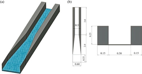
The computational domain is an exact replica of the experimental set-up. The flow domain is 4.0 m long, 0.6 m wide at the inlet and 0.3 m wide at the outlet, giving a contraction ratio of 2:1. The immersed boundary method enforces the no-slip condition in the contraction starting at 0.55 m from the inlet, at an angle of $6^{\circ }$ angle and stretches until 2.0 m. The following narrow rectangular channel is 2.0 m long and 0.15 m wide. The initial water depth is set to 0.03 m and the prescribed bulk velocity $U_b$ matches a discharge of 0.041 m${}^3$ s${}^{-1}$. This yields a bulk Reynolds number, R, of 130,000. The corresponding Froude number, F, is 4.01. The pressure gradient between upstream and downstream end yields a global (domain-averaged) bed shear-stress, $〈\tau 〉=0.45$ N m${}^{-2}$ and global shear velocity of $u_{\ast }=0.02$ m s${}^{-1}$. At the inlet, a constant velocity inflow boundary condition is used and a convective boundary condition is used at the outlet. The experiment used a sluice gate at the inlet with a rather unknown velocity profile, and turbulent fluctuations could be a source of inaccuracy when numerical results are compared with experimental data. No-slip boundary conditions are used at side walls and the bottom of the domain. The level-set method with the initial location of the free-surface at 0.03 m was used to compute the water surface elevation. The selected grid is uniform and the grid resolution is provided in Table 1. The number of points in the three spatial directions are $800\times 240\times 100$ in x, y and z-direction, respectively. The grid features a 2:1:1 aspect ratio and spacings in wall-units are $\mathrm{\Delta }{x}^{+}=50$, $\mathrm{\Delta }{y}^{+}=25$ and $\mathrm{\Delta }{z}^{+}=25$, and approximately half of these numbers near the bottom and side walls. Time-averaging of turbulence statistics is commenced after approximately 24 eddy turnover times ($t_e=H/u_{\ast }$), where H is the water depth.

Table 1. Grid resolution

Points in x	800	dx	0.005	$\mathrm{\Delta }{x}^{+}$	50
Points in y	240	dy	0.0025	$\mathrm{\Delta }{y}^{+}$	25
Points in z	100	dz	0.0025	$\mathrm{\Delta }{z}^{+}$	25

4. Results and discussion

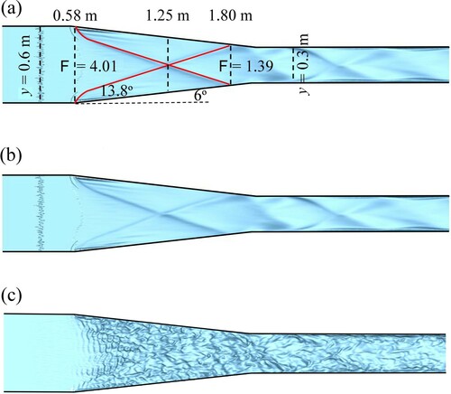
Figure 2a quantifies the shockwaves originating at x = 0.58 m, i.e. shortly after the start of the contracting section. At a contraction angle of $6^{\circ }$ the shockwaves are angled at ${13.8}^{\circ }$ and hence reattach before the contracting section ends at approximately x = 1.8 m with a crossover point at x = 1.25 m. Figure 2b visualizes the time-averaged and Fig. 2c the instantaneous water surface in the open channel. As the flow enters the contraction, shockwaves are generated at either of the contraction edges. These are well defined on the time-averaged plot, but not very obvious on the instantaneous plot due to the strong turbulence prevailing. As the contraction angle is relatively mild, the angles of the shockwaves are mild too and hence the two waves cover almost the entire contraction. The angle of the reflecting waves, which occur in the narrow section, are steeper and waves are shorter. The amplitude decreases towards the outlet, as reflected shockwaves dissipate.

Figure 2. Visualization of surface waves: (a) shock-wave geometry; (b) time-averaged water surface; (c) instantaneous water surface

4.1. Validation

The experimental data presented in Abdo et al. (2019) are used to validate the simulations in terms of water surface profiles. In the experiment, water surface profiles were taken along two longitudinal locations. The first profile was taken at y = 0.3 m, referred to as the centreline profile, and the second profile was taken at a distance 0.08 m from the wall, referred to as the near-wall profile. The experimental data and the results from the 3D RANS simulation by Abdo et al. (2019) are plotted together with the current LES results in Fig. 3. The LES-predicted water surface profiles show satisfactory agreement with the experimental data for the centreline profile, Fig. 3a. The LES predicts the water surface at the entrance to and within the contraction remarkably well, whereas the water surface is approximately overestimated by 5% from the cross-over point towards the end of the contraction. The (standing) reflected shock waves in the narrow channel are captured reasonably well by the LES; wave amplitude and positions of the wave crossovers are slightly underestimated, however; the LES offers similar predictions to the RANS simulation results of Abdo et al. (2019). The RMS error of the water surface in the centreline compared to the experimental values for the LES simulation is 0.01, which is the same as the RMS error obtained from the RANS simulation presented by Abdo et al. (2019).

Figure 3. Measured and LES- and RANS-computed water surface profiles along: (a) centreline; (b) near the sidewall

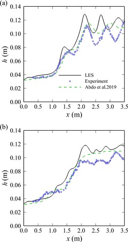
From the near-wall water surface profile shown in Fig. 3b, it can be seen that the LES follows the same trend as the experimental data albeit slightly (roughly 10%) overestimated water levels. The near-wall water surface RMS error compared to the experimental values for the LES simulation is 0.011, which is slightly higher than the RMS error of 0.08 obtained from the RANS simulation presented by Abdo et al. (2019). The presence of the shockwaves is captured and provides improvements of the Abdo et al. (2019) RANS model predictions in terms of capturing the waves near the wall. In the LES, the origin of the primary shockwave is slightly shifted towards the upstream in comparison to the experiment, potentially the result of the treatment of the wall using immersed boundaries. The origin of the shockwave is very sensitive to the near-wall acceleration of the flow and the boundary layer contraction and probably a substantially finer grid (than the one employed) would have been required ; however, at the time of performing the simulations such a grid was deemed too expensive. The reflected shockwaves near the wall in the contracted section of the channel are captured by the LES, an improvement over the RANS results, but the water levels are slightly overestimated.

4.2. Time-averaged flow

Figure 4 presents contours of the time-averaged streamwise velocity in horizontal and longitudinal planes. The streamwise velocity changes from a very shallow fast flow to a deeper slower flow in the narrow section due to the disproportional increase of water depth relative to the decrease in channel width. The distribution of the time-averaged streamwise velocity, normalized by the bulk velocity, near the bed and near the water surface are shown in Fig. 5a and b, respectively, and in a longitudinal plane in Fig. 5c. Because the bed is not sloped and the water level is constantly rising, the maximum velocity is at the inlet and it reduces towards the outlet. Noteworthy are pockets of high velocity near the bed and near the sidewalls and low velocities underneath the shockwaves, reflecting the non-uniform water surface distribution across the channel. The significant rise of the water surface is obvious in the longitudinal plane plot. The high velocity from the inlet reduces rapidly, also noticeable is the growth of the boundary layer after x = 1.0 m. Very low streamwise velocities are observed in the troughs between standing waves.

Figure 4. Time-averaged streamwise velocity distributions in: (a) horizontal plane near the bed at $z/h=0.1$; (b) horizontal plane near the water surface distribution at $z/h=0.9$ (c) longitudinal plane in the centreline

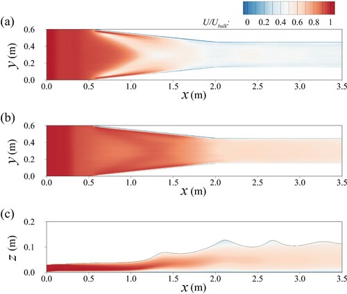
Figure 5. Contours of the time-averaged streamwise velocity at selected cross-sections

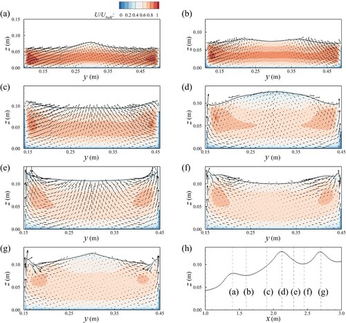
The distributions of the time-averaged streamwise velocity at selected cross-sections in the contraction are presented in Fig. 5. The plots indicate strong momentum at the beginning of the contraction (a) and high-momentum fluid from near the channel walls, where the flow depth is lower than in the centreline, is being transported towards the centreline, which is where the water surface rises and forms (standing) waves. At location (b), it can be noted that the flow is directed towards the walls as the water surface in the centreline is in a trough. At location (c), strong up-flow near the water surface is observed, as expected, as the water surface increases rapidly. The peak of the second standing-wave is presented at point (d), at which fluid is returning towards the walls due to the significant water surface gradient from the centre to the wall. The water surface is depressed between shockwaves and recirculation zones near the wall corners are observed. In the narrow channel, the reflected waves on either side wall result in near surface flow towards the walls where the water surface rises again, as seen in locations (e), (f) and (g). Pockets of high streamwise velocity occur near the walls. As can be seen, the non-uniformity of the water surface in the entire channel is responsible for significant secondary circulation in the cross-section, which in turn results in a non-uniform streamwise velocity distribution in the cross-section.

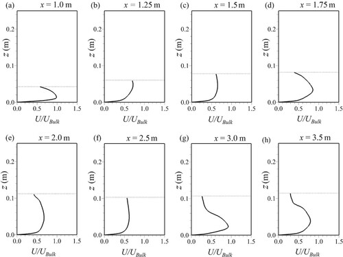
Streamwise velocity profiles in the channel centre at several locations along the domain are plotted in Fig. 6. The velocities are normalized by the local bulk velocity. The flow has a constant inflow at the inlet and as it approaches the contraction, the flow accelerates. The velocity profile is not logarithmic due to the strong secondary flow and the peak of the velocity profile occurs well below the water surface. This is depicted in profiles at x = 1.0, x = 1.25, x = 1.75, x = 3.0 and x = 3.5 m. The maximum near surface velocity is located at x = 1.25 m, the middle of the contracting section and the highest near-bed velocity is found at x = 3.0 m, i.e. in the through downstream of the reflected shockwave which is the result of high-momentum being transported from the corners of the channel towards the centre. In the narrow section, higher velocities are found near the bed rather than near the surface. Figure 6 illustrates that the flow velocity profiles depend strongly on the location of the shockwave crossover point and locations of where the flow maintains its upstream Froude number inside the shockwaves.

Figure 6. Time-averaged streamwise velocity profiles in the contraction, at selected locations along the channel centreline

4.3. Second order statistics and shear stresses

The spatial distribution of the turbulent kinetic energy (tke) in a horizontal plane near the bed is shown in Fig. 7a. The turbulent kinetic energy is normalized by the squared bulk shear velocity, which is $u_{\ast }=0.02$ m s${}^{-1}$. Regions of high kinetic energy occur in the contraction, where the water surface rises and in particular below the shockwaves and downstream of the location of the shockwave crossover. The turbulent kinetic energy reduces gradually once the flow has reached the narrow channel at x = 2.0 m. Figure 7a shows that the turbulent kinetic energy reaches peaks of up to 150 times the squared mean shear velocity between x = 1.0 and x = 1.5 m, which is the location in the domain where the peak of the streamwise velocities is well below the water surface and steep velocity gradients prevail.

Figure 7. Contours in the horizontal plane near the bed at z/h = 0.1 of: (a) turbulent kinetic energy; (b) streamwise normal stress; (c) spanwise normal stress; (d) vertical normal stress

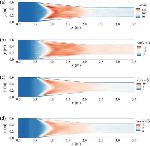
Figure 7b, c and d presents contours of the normalized normal stresses in the streamwise, spanwise and vertical direction, respectively, in a horizontal plane near the bed. The largest contributor to the turbulent kinetic energy is the streamwise normal Reynolds stress. The normalized $u^{\prime }{u}^{\prime }$ stress reaches 15 times the squared shear velocity, and this peak is observed at the same location where the flow attains the maximum velocity acceleration, which is in the middle of the contracting section, i.e. where the two shockwaves cross over and where the water surface is depressed. The streamwise normal stress drops to half of its maximum value as the flow approaches the outlet.

The spanwise normal Reynolds stress also reaches its maximum at the point where the rise in the water level has the largest gradient, i.e. at the shockwave crossover as shown in Fig. 7c. However, as expected, the spanwise Reynold's stresses $v^{\prime }{v}^{\prime }$ are significantly smaller than the streamwise stresses, with the maximum values of $\sqrt{v^{\prime }{v}^{\prime }/u_{\ast }^2}\approx 10$. The stress drops to a quarter of its peak near the outlet. Contours of the vertical normal stresses $\sqrt{w^{\prime }{w}^{\prime }}$ near the bed are presented in Fig. 7d. Similar to before, values increase as the flow accelerates and the peak is at the same location as for the other two components. Peak stresses of $\sqrt{w^{\prime }{w}^{\prime }/u_{\ast }^2}\approx 4$ are observed. The peak is reduced by a factor of 2 towards the outlet.

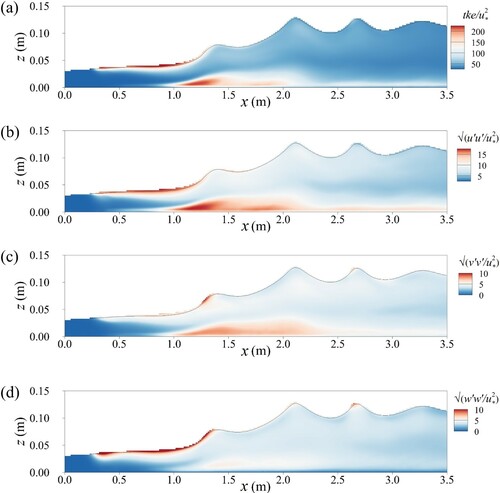
Turbulent kinetic energy, normal streamwise, spanwise and vertical stresses in a longitudinal plane in the centreline (y = 0.3 m) are shown in Fig. 8. The turbulent kinetic energy peaks near the water surface as the flow enters the contraction and a shear layer forms due to the significant velocity gradients prevailing between the peak velocity at approximately half depth and the water surface. As the water surface rises rapidly in the contraction this peaks gradually dissipates until the shockwave cross-over point at $x\approx 1.3$ m. The maximum turbulent kinetic energy near the bed develops below the shockwaves and as a result of high-momentum fluid at half channel depth, entailing a strong velocity gradient near the bed. The largest contributor to both the near-bed and near-surface tke is the streamwise normal stress; however, in the contraction the vertical normal Reynolds stress near the water surface is of the same order as the streamwise normal stress quantifying the strong momentum transfer in the wall-normal direction in this area.

Figure 8. Contours in a longitudinal plane at y = 0.3 m: (a) turbulent kinetic energy; (b) streamwise normal stress; (c) spanwise normal stress; (d) vertical normal stress

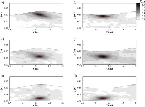
Contours of the two-point correlation function of the streamwise velocity fluctuation in the longitudinal centre plane are presented in Fig. 9. The reference points are placed at three different depths (near bed, half depth, near surface) and two different streamwise locations (second shockwave cross-over and trough thereafter) and the red lines indicate the direction of correlated turbulence. Near the bed turbulence structures are inclined at a relatively shallow angle consistent with boundary layer turbulence transporting low momentum fluid away from the wall. The visualized structures in the centre of the channel are inclined negatively, i.e. transporting high momentum fluid towards the wall, and exhibit coherence over at least three to four water depths, and the auto-correlations look similar for both locations. Near the water surface the structures below the shockwave cross-over exhibit a significant downwards direction, a result of the secondary (down) flow at this location and aided by the water surface gradient. In the trough the turbulence structures are almost parallel to the water surface and very little down-flow is observed. The near-surface structures exhibit coherence over at least six water depths irrespective of streamwise location.

Figure 9. Two-point spatial correlation (streamwise)

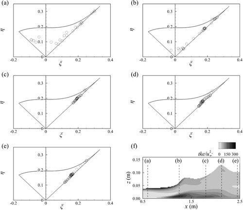
The second (η) and third (ξ) invariants of the Reynolds stress anisotropy tensor (e.g. Simonsen & Krogstad, 2005) along the vertical direction at various locations are plotted inside a Lumley triangle in Fig. 10. The origin represents isotropic turbulence, the left corner point is the area of two-component axisymmetric turbulence, and the right corner is the area of one-component turbulence. At location (a), the beginning of the contraction, the flow starts to decelerate and the profile exhibits some two-component turbulence mid-depth owing to shift of the high-velocity near the surface towards the middle of the channel. At (b) strong boundary layer turbulence is observed near the bed due to the wall shear and near the water surface reflecting its fluctuation due to the shockwaves and the turbulence tends to be mainly axi-symmetric ($\xi >0$) and 1-component turbulence close to the boundaries, whereas in the channel centre the turbulence is trending towards the origin, i.e. is close to isotropic. The flow is pretty much anisotropic over its entire depth at locations (c), (d) and (e). At these locations all values are very close to the axisymmetric boundary, similar to boundary layer flows, however without the presence of a log-layer in which more isotropic turbulence is found. The structures at these locations can be described as axisymmetric rod-like turbulence, or elongated structures, and there is a dominance of the streamwise velocity fluctuation a sign of the breakdown of high and low-speed streaks which is typical of a decelerating flow.

Figure 10. Lumley triangle plotted in a ξ-η plane

4.4. Pressure coefficient and energy line

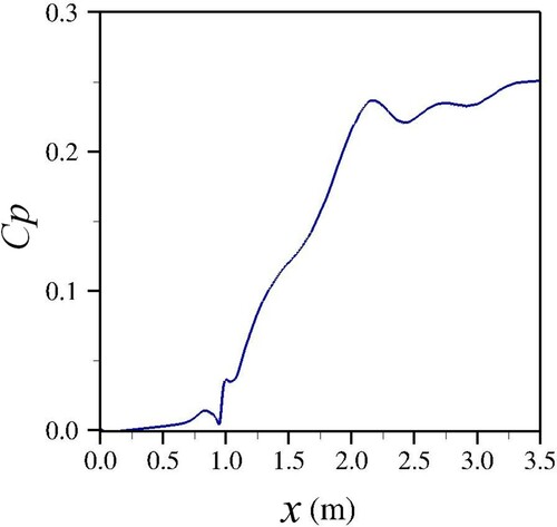
The pressure coefficient, $C_p$, is taken near the bed and is calculated along the domain centreline. The centreline profile of the pressure coefficient is plotted in Fig. 11. The distribution indicates that the coefficient rises as the channel contracts from 0.6 m spanwise width to 0.3 m width. As expected, the reduction of flow area and the rise of the water surface results in a rise of the pressure coefficient along the domain. (3) $C_p=\frac{P-P_0}{0.5\ast \rho \ast U_0^2}$(3) The specific energy E is obtained using Eq. (4(4) $E=z+\frac{U^2}{2g}$(4) ) and it is plotted as a function of streamwise distance from the channel inlet in Fig. 12. The energy generally drops from the inlet to outlet of the domain; however, the drop is very mild in the wide and narrow channel sections and significant in the contraction. The total head loss can be calculated from the energy at the domain inlet and the energy at the domain outlet. The total head loss along the domain is 0.11 m and 97% of it occurs in the contraction. Noteworthy are the plateaus of the energy line around the shockwave crossover and the reattachment point of the shockwaves, respectively. The computation of the pressure coefficient and the energy loss in contractions is motivated by the use of novel hydrokinetic turbine systems (Adzic et al., 2020), investigating how a certain contraction angle reduces the kinetic energy of the flow fed to the turbine runner. (4) $E=z+\frac{U^2}{2g}$(4)

Figure 11. Centreline profile of the pressure coefficient

4.5. Drag forces

The total drag force on the contraction consists of friction or viscous drag force as well as the pressure or form drag force resulting from the pressure gradient. 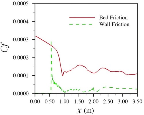The results shown in this section are spanwise averaged: (5) $\begin{array}{rl}Cf& =\frac{F_{\mu }}{0.5\ast \rho \ast {U_{bulk}}^2}\end{array}$(5) (6) $\begin{array}{rl}C{p}_d& =\frac{F_p}{0.5\ast \rho \ast {U_{bulk}}^2}\end{array}$(6) The viscous drag, $F_{\mu }$ is calculated from bed shear stress $\mu (\mathrm{\partial }U/\mathrm{\partial }z+\mathrm{\partial }V/\mathrm{\partial }z)$ and side wall shear stress $\mu (\mathrm{\partial }U/\mathrm{\partial }y+\mathrm{\partial }V/\mathrm{\partial }y)$ and these are plotted as a function of x in Fig. 13. Generally, the bed friction coefficient is larger than the side wall friction coefficient. The bed friction coefficient becomes more uniform as the flow approaches the outlet. The wall friction coefficient peaks at the beginning of the contraction due to the sudden flow acceleration and formation of shockwaves it then reduces towards the centre of the contraction and remains constant until the outlet.

Figure 12. Energy line of spanwise averaged flow along the x-direction

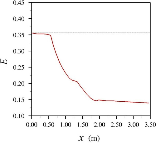
Figure 13. Viscous drag coefficient from bed and walls

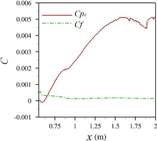
Form drag, $F_p$ is calculated for the contraction side walls for x = 0.55 to 2 m. The pressure gradient over the length of the contracting side walls is integrated over the flow depth. The form drag coefficient $C{p}_d$, shown in Fig. 14, peaks at the centre of the contracting sides. As the contraction approaches a uniform width, the form coefficient also becomes more uniform. This is to be expected as the form drag in the uniform 0.3 m width section is constant due to the flow being parallel to the domain sides. Because of the high Reynolds number in the flow, the form drag on the sides of the contraction is significantly larger than the viscous drag. The minimum friction drag coefficient is at about 2% of the form drag coefficient at $x=1.5$ m. The maximum friction drag coefficient is about nine times larger than the form drag coefficient at the start of the contraction, at the location of the sharp corner.

Figure 14. Viscous (Cf) and form drag ($C{p}_d$) coefficients in the contraction

5. Conclusions

The method of large-eddy simulation in combination with level-set and immersed boundary methods were employed to simulate supercritical flow in a straight-wall open-channel contraction. The LES was validated first with experimental data in terms of water level along the channel and simulated water levels agree reasonably well with measured data. The formation of a pair of shockwaves, a common water surface feature in channel contractions is quite accurately obtained as well as subsequent reflected waves in the narrow section of the channel.

The time-averaged flow is significantly affected by the contracted flow, the water level rise and the presence of shockwaves: the cross-sectional-averaged streamwise velocity is reduced due to the water levels rising faster than the reduction in channel width, leading to a deceleration of the flow. The velocity profiles in the contraction and the ensuing outlet section deviate significantly from a logarithmic profile due to the presence of strong secondary currents and the peak of the streamwise velocity occurs well below the water surface. Contour plots of the second order statistics in terms of tke and its three normal stress contributors confirmed that the highest turbulence occurs in the vicinity of the shockwave crossover location, which is where the maximum streamwise velocity gradients are found. Strong turbulence is also observed near the water surface in the vicinity of the shockwaves as a result of their unsteady behaviour. The two-point auto-correlation functions in space showed and quantified the occurrence of large-scale turbulence structures, the largest of which are generated near the water surface, due to their significant dynamics and which are directed towards the centre of the channel. The analysis of the anisotropy of the Reynolds stress employing the well-known Lumley triangle suggests strong turbulence anisotropy in the entire flow and in particular a dominance of rod-like axisymmetric turbulence as the flow decelerates in the contraction, which is where the streamwise velocity fluctuations dominate the Reynolds stress tensor. The energy line and drag force analyses suggest that the flow loses the majority of its energy in the form of pressure drag.

Notation

Cf	=	friction coefficient (−)
Cp	=	pressure coefficient (−)
$C{p}_d$	=	form drag coefficient (−)
d	=	distance function (−)
E	=	specific energy (m)
f	=	volume force from immersed boundary points (N/m3)
$\mathsf{\text{F}}$	=	Froude number (–)
$F_{\mu }$	=	viscous drag force (N)
$F_p$	=	form drag force (N)
H	=	flow depth (m)
$H\left(\varphi \right)$	=	Heaviside function (−)
L	=	reference length scale (m)
p	=	pressure (Pa)
Q	=	flow discharge (m${}^3$ s${}^{-1}$)
$\mathsf{\text{R}}$	=	Reynolds number (–)
$s\left(d_0\right)$	=	smoothed sign function (−)
t	=	time (s)
$t_a$	=	artificial time (s)
$t_e$	=	eddy turnover time (s)
tke	=	turbulent kinetic energy
u	=	the velocity vector (m s${}^{-1}$)
$u_{\ast }$	=	shear velocity (m s${}^{-1}$)
$u^{\prime }{u}^{\prime }$	=	streamwise normal Reynolds stress (N/m2)
$u^{\prime }{w}^{\prime }$	=	primary shear Reynolds stress (N/m2)
U	=	flow velocity (m s${}^{-1}$)
U	=	time-averaged streamwise velocity (m s${}^{-1}$)
$U_{bulk}$	=	bulk velocity (m s${}^{-1}$)
$v^{\prime }{v}^{\prime }$	=	spanwise normal Reynolds stress (N/m2)
V	=	time-averaged spanwise velocity (m s${}^{-1}$)
ε	=	half thickness of the interface (m)
${ϵ}_r$	=	single grid space (m)
${\mu }_g$	=	dynamic viscosity of gas (kg m s${}^{-1}$)
${\mu }_l$	=	dynamic viscosity of liquid (kg m s${}^{-1}$)
ν	=	kinematic viscosity (m${}^2$/s)
ϕ	=	level-set distance function (−)
${\rho }_g$	=	density of gas (kg m${}^{-3}$)
${\rho }_l$	=	density of liquid (kg m${}^{-3}$)
τ	=	bed shear stress (Pa)
$\mathrm{\nabla }\mathit{\tau }$	=	sub-grid scale stress tensor (−)
$\Gamma$	=	interface between gas and liquid domains (−)
${\Omega }_{gas}$	=	gas fluid domain (−)
${\Omega }_{liquid}$	=	liquid fluid domain (−)

Acknowledgments

The computations presented in this paper were carried out on Cardiff University's Hawk High Performance Computing Wales system.

Disclosure statement

No potential conflict of interest was reported by the authors.

Additional information

Funding

This research is funded by Emrgy Inc. Atlanta and Cardiff University School of Engineering.

References

- Abdo, K, Riahi-Nezhad, C. K., & Imran, J. (2019). Steady supercritical flow in a straight-wall open-channel contraction. Journal of Hydraulic Research, 57(5), 647–661. https://doi.org/https://doi.org/10.1080/00221686.2018.1504126
- Adzic, F., Stoesser, T., Morris, E., & Runge, S. (2020). Design and performance of a novel spillway turbine. Journal of Power and Energy Engineering, 8(5), 14–31. https://doi.org/https://doi.org/10.4236/jpee.2020.85002
- Alcrudo, F., & Garcia-Navarro, P. (1993). A high-resolution Godunov type scheme in finite volumes for the 2D shallow-water equations. International Journal of Numerical Methods and Fluids, 16(6), 489–505. https://doi.org/https://doi.org/10.1002/(ISSN)1097-0363
- Alessandrini, B., & Delhommeau, G. A. (1996). A multigrid velocity-pressure free-surface-elevation fully coupled solver for calculation of turbulent incompressible flow around a hull. Proceedings of the 21th Symposium on Naval Hydrodynamics), Trondheim, Norway.
- Berger, R., & Stockstill, R. (1993). Finite-element model for high velocity channels. Journal of Hydraulic Engineering, 121(10), 710–716. https://doi.org/https://doi.org/10.1061/(ASCE)0733-9429(1995)121:10(710)
- Bhalamudi, S. M., & Chaudhry, M. H. (1992). Computation of flows in open-channel transitions. Journal of Hydraulic Research, 30(1), 77–93. https://doi.org/https://doi.org/10.1080/00221689209498948
- Bomminayuni, S., & Stoesser, T. (2011). Turbulence statistics of open-channel flow over a rough bed. Journal of Hydraulic Engineering, 137(11), 1347–1358. https://doi.org/https://doi.org/10.1061/(ASCE)HY.1943-7900.0000454
- Boris, J. P., & Book, D. L. (1973). Flux-corrected transport. I. SHASTA, a fluid transport algorithm that works. Journal of Computational Physics, 11(1), 38–69. https://doi.org/https://doi.org/10.1016/0021-9991(73)90147-2
- Bradford, S., & Katopodes, N. (1999). Hydrodynamics of turbid underflows I: Formulation and numerical analysis. Journal of Hydraulic Engineering, 125(10), 1006–1015. https://doi.org/https://doi.org/10.1061/(ASCE)0733-9429(1999)125:10(1006)
- Bradford, S., & Sanders, B. F. (2002). Finite-volume model for shallow-water flooding of arbitrary topography. Journal of Hydraulic Engineering, 128(3), 289–298. https://doi.org/https://doi.org/10.1061/(ASCE)0733-9429(2002)128:3(289)
- Causon, D., Mingham, C., & Ingram, D. (1999). Advances in calculation methods for supercritical flow in spillway channels. Journal of Hydraulic Engineering, 125(10), 1039–1050. https://doi.org/https://doi.org/10.1061/(ASCE)0733-9429(1999)125:10(1039)
- Chang, Y. C, Hou, T. Y., Merriman, B., & Osher, S. (1996). A level set formulation of Eulerian interface capturing methods for incompressible fluids. Journal of Computational Physics, 124(2), 449–464. https://doi.org/https://doi.org/10.1006/jcph.1996.0072
- Chow, V. T. (1959). Open-channel hydraulics. McGraw-Hill Book Co..
- Chua, K. V., Fraga, B., Stoesser, T., Hong, S. H., & Sturm, T. (2019). Effect of bridge abutment length on turbulence structure and flow through the opening. Journal of Hydraulic Engineering, 145(6), 04019024. https://doi.org/https://doi.org/10.1061/(ASCE)HY.1943-7900.0001591
- Daly, B. J. (1967). Numerical study of two fluid Rayleigh-Taylor instability. Physics of Fluids, 10(2), 297–307. https://doi.org/https://doi.org/10.1063/1.1762109
- Dawson, J. H. (1943). The Effect of lateral contractions on super-critical flow in open-channels [Master's theses]. Lehigh University.
- Fadlun, E., Verzicco, R., Orlandi, P., & Mohd-Yusof, J. (2000). Combined immersed-boundary finite-difference methods for three-dimensional complex flow simulations. Journal of Computational Physics, 161(1), 35–60. https://doi.org/https://doi.org/10.1006/jcph.2000.6484
- Farmer, J., Martinelli, L., & Jameson, A. (1993). A fast multigrid method for the non-linear ship wave problem with a free surface. Proceedings of the Sixth International Conference on Numerical Ship Hydrodynamics, Iowa, USA, 1993 (pp. 155-172).
- Ferziger, J., & Perić, M. (2002). Computational methods for fluid dynamics. Springer-Verlag.
- Fulgosi, M., Lakehal, D., Banerjee, S., & de Angelis, V. (2003). Direct numerical simulation of turbulance in a sheared air-water flow with a deformable interface. Journal of Fluid Mechanics, 482(482), 319–345. https://doi.org/https://doi.org/10.1017/S0022112003004154
- Gharangik, A. M., & Chaudhry, M. H. (1991). Numerical simulation of hydraulic jump. Journal of Hydraulic Engineering, 117(9), 1195–1211. https://doi.org/https://doi.org/10.1061/(ASCE)0733-9429(1991)117:9(1195)
- Harlow, F. H., & Welch, J. E. (1965). Numerical calculation of time-dependant viscous incompressible flow of fluid with free surface. The Physics of Fluids, 8(12), 2182–2189. https://doi.org/https://doi.org/10.1063/1.1761178
- Hirt, C. W., & Nichols, B. D. (1981). Volume of fluid (VOF) method for the dynamics of free boundaries. Journal of Computational Physics, 39(1), 205–225. https://doi.org/https://doi.org/10.1016/0021-9991(81)90145-5
- Hodges, B. R., & Street, R. L. (1999). On simulation of turbulent non-linear free-surface flows. Journal of Computational Physics, 151(2), 425–457. https://doi.org/https://doi.org/10.1006/jcph.1998.6166
- Hsu, M., Ten, W., & Lai, C. (1998). Numerical simulation of supercritical shock wave in channel contraction. Computers & Fluids, 27(3), 347–365. https://doi.org/https://doi.org/10.1016/S0045-7930(97)00068-6
- Ippen, A. T., & Dawson, J. H. (1951). High-velocity flow in open-channels: A symposium: Design of channel contractions. Transactions of the American Society of Civil Engineers, 116(1), 326–346. https://doi.org/https://doi.org/10.1061/TACEAT.0006522
- Jeon, J., Lee, J. Y., & Kang, S. (2018). Experimental investigation of three-dimensional flow structure and turbulent flow mechanisms around a nonsubmerged spur dike with a low length-to-depth ratio. Water Resources Research, 54(5), 3530–3556. https://doi.org/https://doi.org/10.1029/2017WR021582
- Jiménez, O. F. (1987). Computation of supercritical flow in open channels [Master's theses]. Washington State University.
- Jiménez, O. F., & Chaudhry, M. H. (1988). Computation of supercritical free-surface flows. Journal of Hydraulic Engineering, 114(1), 377–395. https://doi.org/https://doi.org/10.1061/(ASCE)0733-9429(1988)114:4(377)
- Kara, M., Stoesser, T., & McSherry, R. (2015). Calculation of fluid-structure interaction: Methods, refinements, applications. Proceedings of the Institution of Civil Engineers. Engineering and Computational Mechanics, 168(2), 59–78. https://doi.org/https://doi.org/10.1680/eacm.15.00010
- Kara, S., Kara, M. C., Stoesser, T., & Sturm, T. W. (2015). Free-surface versus rigid-lid LES computations for bridge-abutment flow. Journal of Hydraulic Engineering, 141(9), 04015019. https://doi.org/https://doi.org/10.1061/(ASCE)HY.1943-7900.0001028
- Kang, S., & Sotiropoulos, F. (2015). Large eddy simulation of three-dimensional turbulent free surface flow past a complex stream restoration structure. Journal of Hydraulic Engineering, 141(10), 04015022. https://doi.org/https://doi.org/10.1061/(ASCE)HY.1943-7900.0001034
- Kara, S., Stoesser, T., & Sturm, T. W. (2012). Turbulence statistics in compound channels with deep and shallow overbank flows. Journal of Hydraulic Research, 50(5), 482–493. https://doi.org/https://doi.org/10.1080/00221686.2012.724194
- Kara, S., Stoesser, T., Sturm, T. W., & Mulahasan, S. (2015). Flow dynamics through a submerged bridge opening with overtopping. Journal of Hydraulic Research, 53(2), 186–195. https://doi.org/https://doi.org/10.1080/00221686.2014.967821
- Khosronejad, A., Ghazian Arabi, M., Angelidis, D., Bagherizadeh, E., Flora, K., & Farhadzadeh, A. (2019). Comparative hydrodynamics study of rigid-lid and level-set methods for LES of open-channel flows. Journal of Hydraulic Engineering, 145(1), 04018077. https://doi.org/https://doi.org/10.1061/(ASCE)HY.1943-7900.0001546
- Khosronejad, A., Ghazian Arabi, M., Angelidis, D., Bagherizadeh, E., Flora, K., & Farhadzadeh, A. (2020). A comparative study of rigid-lid and level-set methods for LES of open-channel flows: Morphodynamics. Environmental Fluid Mechanics, 20, 145–164. https://doi.org/https://doi.org/10.1007/s10652-019-09703-y
- Kim, D., Kim, J. H., & Stoesser, T. (2010). Large eddy simulation of flow and solute transport in ozone contact chambers. ASCE Journal of Environmental Engineering, 136(1), 22–31. https://doi.org/https://doi.org/10.1061/(ASCE)EE.1943-7870.0000118
- Kim, D., Kim, J. H., & Stoesser, T. (2013). Hydrodynamics, turbulence and solute transport in ozone contact chambers. Journal of Hydraulic Research, 51(5), 558–568. https://doi.org/https://doi.org/10.1080/00221686.2013.777681
- Krüger, S., & Rutschmann, P. (2006). Modelling 3D supercritical flow with extended shallow-water approach. Journal of Hydraulic Engineering, 132(9), 916–926. https://doi.org/https://doi.org/10.1061/(ASCE)0733-9429(2006)132:9(916)
- McKee, S., Tome, M. F., & Ferreira, V. G. (2003). The MAC method. Computers and Fluids, 37(8), 907–930. https://doi.org/https://doi.org/10.1016/j.compfluid.2007.10.006
- McSherry, R., Chua, K., Stoesser, T., & Mulahasan, S. (2018). Free surface flow over square bars at intermediate relative submergence. Journal of Hydraulic Research, 56(6), 825–843. https://doi.org/https://doi.org/10.1080/00221686.2017.1413601
- McSherry, R. J., Chua, K., & Stoesser, T (2017). Large eddy simulation of free-surface flows. Journal of Hydrodynamics, 29(1), 1–12. https://doi.org/https://doi.org/10.1016/S1001-6058(16)60712-6
- Molls, T., & Chaudhry, M. H. (1995). Depth-averaged open channel flow model. Journal of Hydraulic Engineering, 121(6), 453–465. https://doi.org/https://doi.org/10.1061/(ASCE)0733-9429(1995)121:6(453)
- Molls, T., & Zhao, G. (1996). Depth-averaged Bossinesq equations applied to flow in converging channel. North American Water and Environment Congress and Destructive Water (pp. 328–333). ASCE.
- Nichols, B. D., & Hirt, C. W. (1973). Calculating three-dimensional free surface flows in the vicinity of submerged and exposed structures. Journal of Computational Physics, 12(2), 234–246. https://doi.org/https://doi.org/10.1016/S0021-9991(73)80013-0
- Nicoud, F., & Ducros, F. (1999). Subgrid-scale stress modelling based on the square of the velocity gradient tensor. Flow, Turbulence and Combustion, 62(3), 183–200. https://doi.org/https://doi.org/10.1023/A:1009995426001
- Nikora, V., Stoesser, T., Cameron, S. M., Stewart, M., Papadopoulos, K., Ouro, P., McSherry, R., Zampiron, A., Marusic, I., & Falconer, R. A. (2019). Friction factor decomposition for rough-wall flows: Theoretical background and application to open-channel flows. Journal of Fluid Mechanics, 872, 626–664. https://doi.org/https://doi.org/10.1017/jfm.2019.344
- Noh, W. F., & Woodward, P. (1979). SLIC (simple line interface calculations). Lecture Notes in Physics, 59 (pp. 330–340).
- Osher, S., & Sethian, J. A. (1988). Fronts propagating with curvature-dependant speed algorithms based on Hamilton-Jacobi formulations. Journal of Computational Physics, 79(1), 12–49. https://doi.org/https://doi.org/10.1016/0021-9991(88)90002-2
- Ouro, P., Fraga, B., Lopez-Novoa, U., & Stoesser, T. (2019). Scalability of an Eularian-Lagnagian large-eddy simulation solver with hybrid MPI/OpenMP parallelisation. Computers and Fluids, 179(4), 123–136. https://doi.org/https://doi.org/10.1016/j.compfluid.2018.10.013
- Ouro, P., & Stoesser, T. (2019). Impact of environmental turbulence on the performance and loadings of a tidal stream turbine. Flow, Turbulence and Combustion, 102(3), 613–639. https://doi.org/https://doi.org/10.1007/s10494-018-9975-6
- Rahman, M., & Chaudhry, M. H. (1997). Computation of flow in open-channel transitions. Journal of Hydraulic Research, 35(2), 243–256. https://doi.org/https://doi.org/10.1080/00221689709498429
- Raven, H., & Van Brummelen, E. (1999). A new approach to computing steady free-surface viscous flow problems. 1st MARNET-CFD Workshop, Barcelona, Spain.
- Raven, H. C. (1996). A solution method for the nonlinear ship wave resistance problem [Doctoral theses]. Delft University of technology.
- Sanjou, M., & Nezu, I. (2010). Large eddy simulation of compound open-channel flows with emergent vegetation near floodplain edge. 9th International Conference on Hydrodynamics, Shanghai, China (pp. 565–569).
- Shi, J., Thomas, T. G., & Williams, J. J. R. (2000). free-surface effects in open channel flow at moderate Froude and Reynold's numbers. Journal of Hydraulic Research, 38(6), 465–474. https://doi.org/https://doi.org/10.1080/00221680009498300
- Simonsen, A. J., & Krogstad, P. A. (2005). Turbulent stress invariant analysis: Clarification of existing terminology. Physics of Fluids, 17(8), 088103. https://doi.org/https://doi.org/10.1063/1.2009008
- Stoesser, T. (2010). Physically realistic roughness closure scheme to simulate turbulent channel flow over rough beds within the framework of LES. Journal of Hydraulic Engineering, ASCE, 136(10), 812–819. https://doi.org/https://doi.org/10.1061/(ASCE)HY.1943-7900.0000236
- Stoesser, T. (2014). Large-eddy simulation in hydraulics: Quo Vadis? Journal of Hydraulic Research, 25(4), 441–452. https://doi.org/https://doi.org/10.1080/00221686.2014.944227
- Stoesser, T., Braun, C., Garcia-Villalba, M., & Rodi, W. (2008). Turbulence structures in flow over two dimensional dunes. Journal of Hydraulics Engineering, ASCE, 134(1), 42–55. https://doi.org/https://doi.org/10.1061/(ASCE)0733-9429(2008)134:1(42)
- Stoesser, T., McSherry, R., & Fraga, B. (2016). Secondary currents and turbulence over a non-uniformly roughened open-channel bed. Water, 7(9), 4896–4913. https://doi.org/https://doi.org/10.3390/w7094896
- Suh, J., Yang, J., & Stern, F. (2011). The effect of air-water interface on the vortex shedding from a vertical circular cylinder. Journal of Fluids and Structures, 27(1), 1–22. https://doi.org/https://doi.org/10.1016/j.jfluidstructs.2010.09.001
- Ubbink, O. (1997). Numerical prediction of two fluid systems with sharp interfaces [Doctoral theses]. Imperial College of Science, Technology and Medicine.
- Uhlmann, M. (2005). An immersed boundary method with direct forcing for the simulation of particulate flows. Journal of Computational Physics, 209(2), 448–476. https://doi.org/https://doi.org/10.1016/j.jcp.2005.03.017
- Xie, Z. (2015). A two-phase flow model for three-dimensional breaking waves over complex topography. Proceedings of the Royal Society A, 471(2180), 20150101. https://doi.org/https://doi.org/10.1098/rspa.2015.0101
- Xie, Z., Lin, B., & Falconer, R. A. (2014). Turbulence characteristics in free-surface flow over two-dimensional dunes. Journal of Hydro-Environmental Research, 8(3), 200–209. https://doi.org/https://doi.org/10.1016/j.jher.2014.01.002
- Xie, Z., & Stoesser, T. (2020). A three-dimensional Cartesian cut-cell/volume-of-fluid method for two-phase flows with moving bodies. Journal of Computational Physics, 416, 109536. https://doi.org/https://doi.org/10.1016/j.jcp.2020.109536
- Yan, S., Xie, Z., Li, Q., Wang, J., Ma, Q., & Stoesser, T. (2019). Comparative numerical study on focusing wave interaction with FPSO-like structure. International Journal of Offshore and Polar Engineering, 29(2), 149–157. https://doi.org/https://doi.org/10.17736/10535381
- Youngs, D. L., Morton, K. W., & Baines, M. J. (1982). Time-dependent multi-material flow with large fluid distortion. Numerical methods for fluid dynamics (pp. 273–285). Academic Press.
- Yue, W. S., Lin, C. L., & Patel, V. C. (2005). Coherent structures in open-channel flows over a fixed dune. Journal of Fluids Engineering, 127(5), 858–864. https://doi.org/https://doi.org/10.1115/1.1988345
- Zhao, D., Shen, H., Lai, J., & Tabios, G. (1996). Approximate Riemman solvers in FVM for 2D hydraulic shock wave modelling. Journal of Hydraulic Engineering, 122(12), 692–702. https://doi.org/https://doi.org/10.1061/(ASCE)0733-9429(1996)122:12(692)
- Zhao, D., Shen, H., Tabios, G., & Tan, W. (1994). Finite volume two dimensional unsteady flow model for river basins. Journal of Hydraulic Engineering, 120(7), 863–883. https://doi.org/https://doi.org/10.1061/(ASCE)0733-9429(1994)120:7(863)