A base for the log law and von Karman’s constant problem

ABSTRACT

The log-law profile equation and its intrinsic von Karman’s constant are widely used in fluid mechanics. Despite numerous theoretical and empirical attempts to establish formal bases for these concepts, no consensus has been reached. We review past work and present a simple rolling eddy model of boundary-layer turbulence. We consider fluid momentum loss from eddies that roll out over smaller eddies on a timescale that matches the shear interaction of the eddies with the boundary. The resulting parametric form for eddy scaling provides a basis for comprehending turbulent boundary-layer flow as an exponential growth process. The outward-rolling-eddy model formulation yields a log law and explanation for von Karman’s constant. Results of the model are compared with instantaneous flow imagery and direct numerical simulations. The model implies that changes in von Karman’s constant indicate changes in the underlying eddy self-similarity pattern. The approach gives a new perspective on an old problem.

Keywords:

• Attached eddy
• boundary layer
• log law
• turbulent flow
• law of the wall
• velocity profile
• von Karman’s constant

1 Introduction

A boundary layer velocity profile occurs when a moving fluid passes a solid wall (or vice versa) and fluid velocity adjusts to the wall velocity as the wall is approached. For the following investigation, the terms “wall” and “boundary” are used interchangeably.

Near a wall in fully developed, steady, 2-dimensional turbulent fluid flow, the local time-averaged streamwise velocity u_z can be related directly to the shear velocity u* by the logarithm of the perpendicular distance from the wall z. This log law was established by Prandtl and von Karman and the inverse coefficient κ has become known as von Karman’s constant: (1) $\begin{array}{r}{u}_z=\left(u^{\ast }/\kappa \right)\text{ln}\left(z/z_0\right)\end{array}$(1) Here z is measured from the origin of the log profile, z₀ is the distance at which Eq. (1) indicates u_z = 0, $u^{\ast }=\sqrt{\left({\tau }_0/\rho \right)}$ is the shear velocity, τ₀ is the boundary shear stress, ρ is the fluid density and κ ≈ 0.4. The log law has been theoretically justified through mixing length and eddy viscosity concepts (Keulegan, 1938; Prandtl, 1932; Van Driest, 1956), similarity hypotheses (von Karman, 1930), asymptotic matching (Millikan, 1938), dimensional analysis (Buschmann & Gad-el-Hak, 2003) and high-Reynolds-number asymptotic analysis (George & Castillo, 1997; Jimenez & Moser, 2007). It has been advocated for a wide range of wall bounded shear flows by von Karman (1930); Tennekes and Lumley (1972); Hinze (1975); Yaglom (1979) and many others.

Equation (1) has three parameters to determine velocity at a given distance from the wall:

1. z₀ represents the “roughness” of the wall. Viscous effects dominate for smooth boundaries and z₀ ≈ 0.115 υ_m/u* where υ_m is kinematic viscosity of the fluid. For rough, granular boundaries z₀ ≈ k_s/30 where k_s is the wall’s equivalent sand grain roughness (Nikuradse, 1933).

2. u* is the flow momentum sink at the boundary and represents wall shear stress.

3. κ is the von Karman coefficient which has been defined as a universal mixing constant (Pope, 2000; Van Driest, 1956). Because κ operates in an inverse manner to u*, an error in u* can be concealed by adjusting κ and vice versa.

Boundary shear stress is important in many engineering applications ranging from initiation of sediment transport and pipeline pumping costs to global weather prediction models and aircraft performance. When Eq. (1) is used to calculate boundary shear stress from ρu*², a 5% error in κ will result in a ∼ 10% error in τ₀ (other factors held constant). So errors in κ can have significant implications. However, despite the importance of κ and the sensitivity of shear stress calculations to κ, there has been little consensus over the years as to whether κ is, or is not, a “constant”.

2 Empirical values for κ

Nezu and Rodi (1986) measured κ = 0.412 above smooth beds in fully developed open channel flow (OCF). For straight, smooth pipe flow, Long et al. (1993) concluded κ = 0.408 ± 0.004. George (2007) found that κ ≈ 0.38 for classical boundary layer flows and κ ≈ 0.43 for pipe flow and furthermore concluded that a universal log law is not supported by either theory or data. Nagib and Chauhan (2008) also found κ is not universal and exhibits dependence on the pressure gradient and flow geometry, reporting κ ≈ 0.384 in zero-pressure gradient turbulent boundary layers and κ ≈ 0.41 in pipe flows. Marusic et al. (2010) reported on seven comprehensive experimental investigations wherein κ values ranged from 0.37 to 0.421. They noted that Reynolds number dependence of turbulence quantities whenever observed was generally weak.

Direct numerical simulation of boundary layer turbulence reveals κ values that can range from 0.384 ± 0.004 (Lee & Moser, 2015) to 0.452 (She et al., 2017). Atmospheric measurements show κ values as low as 0.35 (Businger et al., 1971) and as high as 0.46 (Sheppard, 1947). While some of this variation may be due to Reynolds number and relative roughness effects, Andreas et al. (2006) claim that atmospheric κ is constant at 0.387 ± 0.003 for a broad range of roughness Reynolds numbers. Other than noting that these empirical studies indicate κ has a value somewhere around 0.4 that is slightly higher for pipe flow than for OCF, there is no clear consensus on an appropriate κ value.

3 Analytical values for κ

Townsend (1976) made a rough calculation of von Karman’s constant by equating eddy viscosity of the mean flow to an eddy-viscosity-equivalent of energy loss from boundary-attached eddies, which led to a value of κ = 0.32. Orsag and Patera (1981) carried out numerical integration of the Navier Stokes equations to calculate κ = 0.46 but cautioned about limitations of their solution. Telford (1982) used “physical principles supporting the entity-entrainment model of turbulent processes in the planetary boundary layer” to calculate κ = 0.369. Yakhot and Orszag (1986) applied a renormalization group method using dynamic scaling and invariance together with iterated perturbation methods to evaluate κ = 0.372, however, Eyink (1994) demonstrated that their neglecting of higher-order terms was not generally viable. Bergmann (1998) assumed that the viscous sublayer and near-wall logarithmic layer velocities and vertical velocity gradients must match at some point, thus implying κ = e^–1 = 0.3678. He claimed “the result for the value of the von Karman constant turns out to be quite a natural constant” (p. 3405); however, his approach has been criticized (Andreas & Trevino, 2000). Hughes (2007) reformulated von Karman’s mixing length theory to consider a length scale over which the mean square of the velocity shear changes, rather than the velocity shear itself. By truncating second derivatives he found $\kappa =\left(\sqrt{2}\text{--}1\right)=0.414$. Baumert (2009) considered shear-generated turbulence at asymptotically high Reynolds numbers for flows comprising dipole vortex tubes. He developed a closed theory without any empirical parameters, with analogies to birth and death processes, which for adiabatic conditions at a solid wall predicted κ = (2π)^−1/2 ≈ 0.399.

These theoretical derivations do not concur, and it is unfortunate that the value of such an important parameter is so elusive. To this list of eclectic calculations and the many unpublished, unsuccessful attempts that have been made to explain κ over the years, we will add below a further simple derivation that for standard conditions κ ≈ 0.405. This result evolves from considering a boundary layer “shear flow” to be a rolling-eddy flow.

4 Conceptual rolling eddy model to explain κ and the log law

To simplify the complex physics of turbulent boundary layer flows, we propose an investigative, conceptual model (Fig. 1) where streamwise flow is governed by eddies rolling with a spanwise axis (or more generally, having a spanwise projected, downstream-rolling component). We will compare this model with previously published visualizations of eddy structures measured in laboratory boundary layers.

Figure 1 A conceptual model of spanwise-axis rolling eddies. Eddies are visualized in the frame of reference of local mean downstream velocity and drawn circular. Eddy tier 1 (blue) is an arbitrary distance d from the boundary. The dotted red boundary eddy at left is rolled out onto tier 1 when its diameter reaches d. The dotted eddy then rolls on tier 1 with its centroid 1.5d from the boundary creating tier 2. The insert illustrates streamwise velocities within fluid elements, size d, without and with a rolling eddy. Flow direction is from left to right

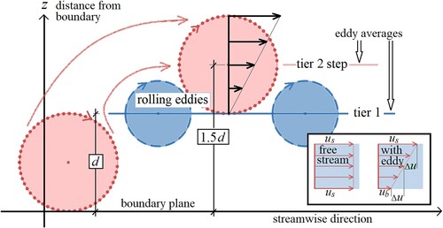
The rolling eddy model has the following assumptions:

1. Rolling eddies grow from the boundary and may roll outward over slower eddies, forming a stack of eddies. This process constrains the downstream velocity.

2. Consider the slower eddy (or stack of eddies) to be rolled over, as a step. We presume a growing boundary eddy with z-dimension d will be dragged by the flow onto an arbitrary step once d reaches the level of the step. The centroid of the out-rolled eddy is then at level 1.5d (Fig. 1) creating a new, higher step.

3. On the insert in Fig. 1 the streamwise velocity within an element of fluid having no boundary influence (on the left) is compared with a similar fluid element containing a clockwise rolling eddy arising from the boundary (shown on the right). The eddy disrupts the free stream and, for the same outer velocity u_s, the mean streamwise velocity of the rolling-eddy element is reduced by an amount Δu compared to the no boundary effect element. For element size d, the streamwise momentum per unit width is reduced by ρ d ²Δu in the case with the rolled-out boundary-generated eddy.

4. The average boundary shear force per unit width over a streamwise boundary distance d (corresponding to our rolling eddy size) is ρu*²d. Only one eddy at a time can interact with a particular point on the boundary and the timescale d/u* is used for this period of interaction.

5. Equating the boundary shear force to the rate of eddy induced streamwise momentum loss gives: ρu*²d = ρd²Δu/(d/u*). This indicates Δu = u* which implies that the centroid of a conceptual rolled-out eddy at z = 1.5d will translate downstream at u* relative to the velocity of its roll plane (u_b on insert in Fig. 1) at z = d.

6. To give a streamwise velocity profile, eddy elements of a given size are averaged as a layer through their centroids, moving downstream at the centroid velocity.

With the above assumptions we have a simple model of turbulent boundary layer flow which infers that the momentum governing spanwise-axis-eddy centroids move streamwise at u* relative to a plane at their base one eddy diameter from the wall. Formulating this result: (2) $\begin{array}{r}{u}_{\left(z\right)}=u^{\ast }+u_{(z-z/3)}\end{array}$(2) The roll plane velocity at (2/3)z is itself governed by rolling eddy behaviour according to Eq. (2). Taking any arbitrary point at coordinates (u = u_ref, z = z_ref) in such a boundary layer, we can find other (u, z) velocity profile points at (u_ref – u*, (2/3)z_ref) and (u_ref – 2 u*, (2/3)²z_ref) and so on, leading to a general parametric velocity profile: (3) $\begin{array}{r}\left(u,z\right)=\left(u_{ref}-n{u}^{\ast },{\left(2/3\right)}^n{z}_{ref}\right)\end{array}$(3) This is shown in Fig. 2a followed by examples from eddy visualization investigations.

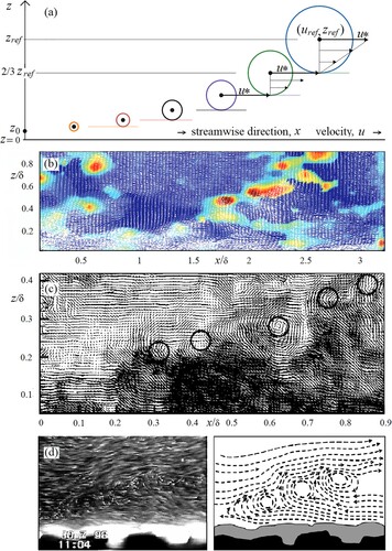
Figure 2 (a) Model results showing Eq. (3) or Eq. (7) with six stacked tiers of spanwise axis eddies rolling at u* relative to roll planes at 2/3rds of their diameter. Images b & c show vortices visualized in a rectangular tunnel (depth 2δ), by Camussi and Di Felice (2006) for momentum thickness Reynolds numbers of 1015 and 17,500 respectively. In b large local intermittency is shown in red and small intermittency is shown in dark blue. In image c “circles evidence the heads of presumed hairpin vortices” in the instantaneous velocity field. Visualization d shows large-scale coherent vortices detected by Cuthbertson and Ervine (2007) “these eddies commonly occurred in pairs or groups each with the same rotational sense, and typically occupied a region of 0.1–0.4 flow depth”. Mean flow directions are from left to right

Taking n = log_2/3(z/z_ref) from the z component and substituting in the u component we convert Eq. (3) to a conventional equation: (4) $\begin{array}{r}{u}_z=u_{ref}\text{--}{u}^{\ast }\text{lo}{\text{g}}_{2/3}\left(z/z_{ref}\right)\end{array}$(4) where the log subscript indicates a log base of 2/3.

If z is assigned a length scale of z₀ where u_z = 0 then Eq. (4) shows u_ref = u*log_2/3(z₀/z_ref).

Substituting for u_ref in Eq. (4) we get: (5) $\begin{array}{rl}{u}_z& =u^{\ast }\text{lo}{\text{g}}_{2/3}\left(z_0/z_{ref}\right)\text{--}{u}^{\ast }\text{lo}{\text{g}}_{2/3}\left(z/z_{ref}\right)\\ & =u^{\ast }\text{lo}{\text{g}}_{2/3}\left(z_0/z\right)=u^{\ast }\text{lo}{\text{g}}_{3/2}\left(z/z_0\right)\end{array}$(5) Applying a change of log base to give natural logs, we arrive at: (6) $\begin{array}{r}{u}_z=\left(u^{\ast }/\kappa \right)\text{ln }\left(z/z_0\right)\text{ where }\kappa =\text{ln}\left(3/2\right)\approx 0.4055\end{array}$(6) which is the von Karman log law.

The eddy propagation occurs outwards from a boundary and Eq. (3) may also be written: (7) $\begin{array}{rl}\left(u,z\right)& =\left(n{u}^{\ast },{\left(1.5\right)}^n{z}_0\right)\end{array}$(7) (8) $\begin{array}{rl}\text{or}z& =z_0(1.5{)}^{u/u^{\ast }}\end{array}$(8) (9) $\begin{array}{rl}\text{or}z/z_0& ={e^{\kappa u}}^{/u^{\ast }}\text{with }\kappa =\text{ln}\left(1.5\right)\end{array}$(9)

5 Discussion

The outward-rolling eddy model assumptions result in a conventional log law without invoking any empirical parameters. In this light, von Karman’s κ is not an elusive constant but, ostensibly, a factor to convert a base 3/2 log to a natural (base e) log. The stacking of eddies evoked by the model and shown in the examples of Fig. 2 is supported by multiple experimental observations, perhaps starting with Meinhart and Adrian (1995) who imaged instantaneous turbulent flow and identified slender regions of intense spanwise-axis vorticity separated by zones of nearly uniform streamwise momentum. The proposed model offers an explanation that out-rolling eddies are responsible for the regions of intense vorticity and cause a drop in streamwise momentum which restricts the streamwise velocity. While discrete layers, steps or tiers are used to explain outward propagation of the rolling eddies, in a real flow, successive stacks of eddy tiers will be transitory and, on average, the parameter n in Eq. (3) or Eq. (7) can be considered to be continuous. In the form of Eq. (8), the eddy model is seen to be an example of an exponential growth process.

The outward-rolling eddy hypothesis was formulated during the time of the COVID-19 global pandemic. As an exercise in lateral thinking, we compare Eq. (8), with the pandemic reproduction formula N = N₀ R^t where N is the number of infected persons, R is the average number of people an infected person goes on to infect and t is the number of generations (or tiers) of infections. Seen as a reproduction formula, Eq. (8) has a R value of 1.5. Continuing the analogy, each u/u* eddy tier facilitates “infection” (or edification?) of a new tier extending 1.5 times the previous distance from the wall as is shown in Fig. 2. By considering the log law as a reproduction formula, without resorting to any eddy hypothesis, we see that κ represents the natural log of the R value. From this perspective, κ will only change if there is a change in the inherent growth process. We investigate implications of changes in κ later in the paper.

The physical assumptions underlying Eq. (2) are that: (i) streamwise velocity in a turbulent boundary flow is governed by fluid momentum loss as eddies get rolled beyond their own diameter from a boundary; and (ii) the timescale for the momentum loss matches the timescale for shear interaction of similarly sized eddies with the boundary. Provided rotation is symmetric within an eddy, it is not essential for rolled-out eddies to have a linear, “solid body” rolling velocity profile as shown in Fig. 1. What is required is that the centre of rotation coincides with the eddy centre of mass at half the effective eddy diameter. The log law profile can then be derived as above, without knowing the specific mechanism of momentum transfer to the boundary. In the framework of a rolling eddy model, such mechanisms could include: (i) rolled out eddies are the heads of hairpin or horseshoe vortices (Fig 2c) which have their legs on the boundary; (ii) rolled out eddies block the flow and displace higher speed fluid back towards the boundary; and/or (iii) downstream rolling eddies are but a spanwise projected component of more complex 3-dimensional flow structures (such as streamwise spirals).

Rotating eddy models have been considered in the past, most notably Townsend’s (1976) concept of attached eddies. A review of the development of attached eddy models is given by Marusic and Monty (2019). The present model, however, relies on the consequences of spanwise-axis rolling eddies that are remote from the bed. As “detached eddy” terminology is often used for regions of separated flow, this term is not used with the present model and, in terms of momentum extraction from the flow, the rolled-out eddies remain “connected” with the boundary. The z-scaling of this model bears some resemblance to the concept of hierarchies of eddies developed by Perry and Chong (1982) who proposed that each eddy dimension doubles, moving away from a boundary, from one hierarchy of eddies to the next. Considering eddy diameter, the present model implies that d_n = (1.5)^n–1z₀ where d_n is the diameter of the nth layer of eddies stratified by u*. Eddy diameter increases by 50% from one u* tier of eddies to the next. In terms of effective eddy diameter as a function of distance from the boundary, d = (2/3)z, i.e. linear growth in eddy geometry with distance from the boundary.

Further away from a boundary, in “outer” regions where boundary influence is diminished or eddy propagation is affected by e.g. a free water surface or the central core region of a closed conduit flow, the z direction increment associated with incremental u* momentum loss could be expected to be influenced relative to near-boundary flow conditions. The centroid to boundary distance of eddies under-the-influence would become smaller or greater than the 1.5 d shown in Fig. 1 depending on whether affected eddies were constrained or expanded. Eq. (8) could become, for example, z = z₀ (1.45)^u/u* or z = z₀ (1.55)^u/u* with corresponding κ values of about 0.37 and 0.44 respectively. This broadening of the rolling eddy concept suggests we could investigate extending the application of the log law outside the conventional range, but with von Karman’s κ value changing in regions where eddy propagation is modulated by secondary influences.

We first consider aspects of the rolling eddy hypothesis in the very-near-boundary region where the log law does not hold and the present model (which produces a log law) could not be expected to apply unmodified. Very close to a smooth boundary, viscous effects suppress eddy formation. For a viscous shear flow the velocity gradient ∂u /∂z is limited to u*² / υ_m with a corresponding linear velocity profile: (10) $\begin{array}{r}{u}_z=\left(u^{\ast 2}/{\upsilon }_m\right)z\text{or}{u}^{+}=z^{+}{z}^{+}<5\end{array}$(10) where, using conventional notation, u⁺ = u/u* and z⁺ =z u* / υ_m. Measurements show that this linear sublayer corresponds roughly to z⁺ < 5 with a buffer transition zone to z⁺ < 25 before unsuppressed rolling that satisfies Eq. (2) could take place.

Close to rough boundaries there is a layer where turbulence and drag from boundary roughness protrusions swamp smaller eddies that would grow outwards from a smooth boundary. In line with the present model, only eddies that exceed the limit of this roughness layer can be rolled out into the flow absorbing momentum in the process. Taking u_r as velocity at the top of a roughness layer at z = δ_r, the model gives: (11) $\begin{array}{rl}{u}_z& =u_r+u^{\ast }\text{lo}{\text{g}}_{3/2}\left(z/{\delta }_r\right)\\ & =u_r+\left(u^{\ast }/\kappa \right)\text{ln }\left(z/{\delta }_r\right)z\ge {\delta }_r,\kappa =\text{ln}\left(1.5\right)\end{array}$(11) This reverts to Eq. (1) with a de-facto roughness scale $z_0={\delta }_r{e}^{-\kappa u_r/u^{\ast }}$ as if there is a virtual log law profile extending back into the roughness layer. Within the roughness layer the eddy structures roll over protrusions and slip along the boundary without permanently leaving the boundary. If these structures have a spanwise-axis forced eddy component, the eddies will roll with a linear streamwise velocity profile, the largest eddies giving a linear velocity profile to the sublayer. For slipping rolling eddies the origin of the linear sublayer will appear to originate from a virtual boundary inside the physical boundary (3).

Figure 3 Streamwise velocity profile on a rough boundary showing model predictions and data measured by Smart et al. (2010) superposed on a diagram showing non-viable blue eddies suppressed within the roughness layer and an eddy of size δ_r rolling out of the roughness layer. Different options for velocity profile datum are indicated

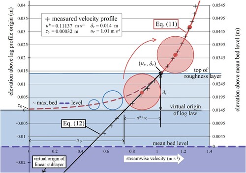
We have at least three options for streamwise velocity profile datum at a rough boundary; z = 0 at the origin of the overlying log law, z = 0 at some measure of the boundary itself (e.g. mean bed level) and z = 0 at the extrapolated origin of the linear sublayer. Depending on the datum, Eq. (1) can be written u_z = (u*/κ)ln((z – a)/z₀) where a is an adjustment to z to offset the chosen origin to match that of the extrapolated log law. Keeping the z = 0 datum at the log law origin, a linear roughness sublayer velocity profile that is continuous with and tangential to the overlying rolling eddy (log law) profile where the profiles meet at the top of the roughness layer (u_r, δ_r), has the equation: (12) $\begin{array}{r}u=u_r-\left(u^{\ast }/\kappa \right)(1-z/{\delta }_r)z\le {\delta }_r\text{linear sublayer}\end{array}$(12) as shown with measured profile data in Fig. 3. The streamwise velocity at the elevation of the log law origin is then u₀ = u_r – (u*/κ) and the virtual origin of the linear sublayer is (κu_r/u*−1)δ_r beneath the origin of the overlying log law. For the rough bed experimental data shown in Fig. 3, Eqs (11) and (12) adequately describe the composite velocity profile using boundary properties δ_r, u_r and u*.

6 Verification

The conceptual model of outward-rolling eddies gives a possible explanation as to how a classical von Karman log-law profile occurs and shows that κ can be considered as a measure of the base of an underlying eddy growth process. However, a sceptical reader may consider that Eq. (8) is an arbitrary coincidence of κ having a value which lies close to ln(3/2). This is a chicken-and-egg debate because a consequence of a κ value close to ln(1.5) means that Eq. (8) closely describes the conventional log law. Resolution could come with exact measurements of κ but reported empirical values differ significantly as described above and independent measurement of u* is not usually accurate enough to determine κ to several significant decimal points.

To circumvent experimental errors in u* causing errors in κ, we investigate using direct numerical simulation (DNS) data where u* is known exactly. The exponential equation: (13) $\begin{array}{r}{z}^{+}=A{e}^{B{u}^{+}}\end{array}$(13) is now fitted to Lee and Moser’s (2015) data for high Reynolds number DNS velocity profiles up to the centreline of a rectangular closed channel. Comparison of Eq. (13) with Eq. (9) shows that A represents z₀/(υ_m/u*) and B represents the value of κ. Results of fitting Eq. (13) are given in Table 1.

Table 1 Log law parameters for three velocity profiles of fully developed turbulent channel flow calculated by DNS

Flow parameters		Log law fitting region range		Indicated log law parameters
Re*	u*	z^+	z/δ	A = f(z^+)	B	R^2
5186	0.0415	56–392	1.1–7.6%	12.88%	0.4052	0.9996
1995	0.0459	41–356	2.0–17.9%	12.64%	0.4055	0.9993
1001	0.0500	39–279	3.9–27.9%	12.46%	0.4054	0.9991
Reδ	u*	z^+	z/δ	A = f(z/δ)	B	R^2
125,000	0.0415	392–4922	7.6–95%	0.5815 × 10^−4	0.3758	0.9991
43478	0.0459	356–1892	17.9–95%	2.356 × 10^−4	0.3647	0.9977
20,000	0.0500	279–948	27.9–95%	4.481 × 10^−4	0.3660	0.9973

${\mathsf{R}\mathsf{e}}_{\ast }$ is the friction Reynold’s number, Re_δ is Reynold’s number based on mean flow, A is the ratio of z₀ to the z-scale parameter, B is the indicated κ value. The z-scaling used is: top three rows, z/(υ_m/u*); bottom three rows, z/δ where δ = half-depth of the closed channel. R² is the fraction of variation in z⁺ that is explained by Eq. (13) using the fitted coefficient values.

For a smooth wall, such as this example, the conventional domain of a log law is found to range from about z⁺ = 30 to z/δ = 0.2 (e.g. Jimenez & Moser, 2007; Lee & Moser, 2015). The first three rows of Table 1 show the optimal range for parameters fitted in this region. The A parameter (z₀⁺) indicates that the roughness length scale z₀ is approximately one eighth of the viscous length scale υ_m/u*. The B parameter shows fitted κ values are extremely close to ln(3/2) or 0.40546. In other words, the DNS data support the conclusions from the outward-rolling eddy model almost exactly within the conventional log law region.

In the bottom three rows of Table 1, the region of fitting is extended out to z/δ = 95%. Extremely good log law profile fits are also obtained in this outer boundary layer region whether z values are scaled as z⁺ or with δ (the same correlation is obtained because each scale parameter remains constant for a given profile). For the outer region the A parameter values show a higher, non-constant relation between z₀ and the viscous length scale or, when based on z/δ, the A values indicate that z₀/δ (relative roughness) increases here with decreasing Reynolds number. While a log law profile is clearly applicable in this outer region, the B parameter indicates lower κ values (around 0.37) and κ displays somewhat wider variation with Re than found closer to the boundary. In terms of our outward-rolling eddy model, this implies that outer region eddies (towards the flow core in this closed channel case) are modulated (slightly squashed) compared to near-boundary eddies that are unaffected by external influences. As e^0.37 ≈ 1.45, a κ = 0.37 value implies that (on average) outer eddies having relative velocity u* roll with centroids at 1.45 d above their roll point instead of at 1.5d as shown in Fig. 1. The DNS data show that this change in eddy behaviour is consistent over the outer 6–8 tiers of u⁺. We can thus regard the Eq. (7) eddy model to be the near-boundary incidence of a more general process, with κ representing the exponential base of the appropriate law relating eddy-z-extent to streamwise velocity. Thinking more profoundly, changes in κ imply changes in the underlying geometric self-similarity of out-rolling eddies.

7 Summary and conclusions

We have presented a 2-dimensional, conceptual model of turbulent boundary layers whereby momentum is lost from the free stream as eddy structures roll outwards from the wall and “stick their heads up” into the flow. We described this eddy propagation in parametric form. The formulation derives the log law and suggests that von Karman’s constant indicates the base of the log law, which gives a new perspective on an old problem. Very close to smooth boundaries viscous effects suppress the rolling behaviour requirement of the model. On rough boundaries a sub-layer develops wherein boundary roughness protrusions disrupt eddy out-rolling. The streamwise velocity profile can then be defined by conditions in the top of the roughness sub-layer. Model predictions are consistent with eddy visualization evidence and DNS velocity profile calculations. The proposed model also provides reasons for comprehending turbulent flow as an exponential growth process. Irrespective of the model concept, considering the log law from the perspective of a reproduction formula shows κ is the log of the R value and changes in κ imply changes in the underlying propagation pattern.

In retrospect, the concept is not new. The sketches of Leonardo da Vinci and the paintings of van Gogh have brought rolling eddy tiers to the eyes of beholders of turbulence for over 700 years.

Notation

A	=	value of z0 /(υm/u*) or z0/δ fitted from DNS data
a	=	z offset of profile measurement origin from the virtual origin of the log law profile (m)
B	=	value of κ fitted from DNS data (–)
dn	=	diameter of the nth layer of eddies (m)
DNS	=	direct numerical simulation
e	=	base of natural logs ≈ 2.718 (–)
ks	=	equivalent sand grain roughness (m)
n	=	eddy tier layer (–)
N	=	number of persons infected by a pandemic (–)
N0	=	initial number of infected persons in a pandemic (–)
OCF	=	open channel flow
R	=	average number of people an infected person goes on to infect in a pandemic (–)
R2	=	square of correlation coefficient = fraction of variance explained by the fitted equation (–)
Reδ	=	Reynolds number = Uδ/υm (–)
${\mathsf{R}\mathsf{e}}_{\ast }$	=	friction Reynolds number = u*δ/υm (–)
t	=	number of generations (or tiers) in reproduction formula (–)
u = uz	=	local mean streamwise velocity (m s–1)
U	=	boundary layer mean streamwise velocity = depth average velocity in OCF (m s–1)
ub	=	streamwise velocity at the base of a rolling eddy (m s–1)
u0	=	streamwise velocity at the log law origin within a roughness layer (m s–1)
u+	=	u/u* (–)
us	=	free stream velocity (m s–1)
uz	=	streamwise velocity at distance z from the boundary (m s–1)
u*	=	wall shear velocity = √(τ0 /ρ) (m s–1)
uref	=	arbitrary velocity reference point in turbulent boundary layer (m s–1)
z	=	perpendicular distance from the boundary wall (m)
z0	=	z distance at which log law uz is zero = wall roughness parameter (m)
z0+	=	z0 u* / υm (–)
zref	=	perpendicular distance of uref from the boundary wall (m)
z+	=	zu* / υm (–)
δ	=	boundary layer outer scale = half-depth of closed channel, full depth of open channel (m)
δr	=	roughness layer thickness measured from origin of log law (m)
κ	=	von Karman constant = factor to convert log base 3/2 to log e base ≈ 0.405 (–)
ρ	=	fluid density (kg m–3)
τ0	=	wall shear stress (kg m–1 s–2)
υm	=	kinematic viscosity of the fluid (m2 s–1)

Acknowledgements

Alan Cuthbertson and Roberto Camussi kindly shared the vortex imagery used in Fig. 2. The Journal reviewers and sub-editor provided significant background references that helped develop the initial version of this work.

Disclosure statement

No potential conflict of interest was reported by the authors.

Additional information

Funding

The research was funded by New Zealand Ministry of Business, Innovation and Employment: ‘Natural Hazards’ research (C05X0907), ‘Drone Flow’ research (C01X1812) and National Institute of Water and Atmospheric Research (NIWA) ‘Environmental Flows’ research (FWWA2103).

References

- Andreas, E. L., Claey, K. J., Jordan, R. E., Fairall, C. W., Guest, P. S., Persson, P. O. G., & Grachev, A. A. (2006). Evaluations of the von Kármán constant in the atmospheric surface layer. Journal of Fluid Mechanics, 559, 117–149. doi:10.1017/S0022112006000164
- Andreas, E. L., & Trevino, G. (2000). Comments on “a physical interpretation of von kármán’s constant based on asymptotic considerations—A new value”. Journal of the Atmospheric Sciences, 57(8), 1189–1192.
- Baumert, H. Z. (2009). Primitive turbulence: kinetics, Prandtl’s mixing length, and von Karman’s constant. arXiv.org 0907.0223v2 [physics.flu-dyn] [Online].
- Bergmann, J. C. (1998). A physical interpretation of von Kármán’s constant based on asymptotic considerations—A new value. Journal of the Atmospheric Sciences, 55(22), 3403–3407. doi:10.1175/1520-0469(1998)055<3403:APIOVK>2.0.CO;2
- Buschmann, M. H., & Gad-el-Hak, M. (2003). Generalized logarithmic law and its consequences. AIAA Journal, 41(1), 40–48. doi:10.2514/2.1911
- Businger, J. A., Wyngaard, J. C., Izumi, Y., & Bradley, E. F. (1971). Flux-profile relationships in the atmospheric surface layer. Journal of the Atmospheric Sciences, 28(2), 181–189. doi:10.1175/1520-0469(1971)028<0181:FPRITA>2.0.CO;2
- Camussi, R., & Di Felice, F. (2006). Statistical properties of vortical structures with spanwise vorticity in zero pressure gradient turbulent boundary layers. Physics of Fluids, 18(3), 035108. doi:10.1063/1.2185684
- Cuthbertson, A. J. S., & Ervine, D. A. (2007). Experimental study of fine sand particle settling in turbulent open channel flows over rough porous beds. Journal of Hydraulic Engineering, 133(8), 905–916. doi:10.1061/(ASCE)0733-9429(2007)133:8(905)
- Eyink, G. L. (1994). The renormalization group method in statistical hydrodynamics. Physics of Fluids, 6(9), 3063–3078. doi:10.1063/1.868131
- George, W. K. (2007). Is there a universal log law for turbulent wall-bounded flows? Philosophical Transactions of the Royal Society A: Mathematical, Physical and Engineering Sciences, 365(1852), 789–806. doi:10.1098/rsta.2006.1941
- George, W. K., & Castillo, L. (1997). Zero-pressure-gradient turbulent boundary layer. Applied Mechanics Reviews, 50(12), 689–729. doi:10.1115/1.3101858
- Hinze, J. O. (1975). Turbulence (2nd ed). McGraw-Hill.
- Hughes, R. L. (2007). A mathematical determination of von Karman’s constant, κ. Journal of Hydraulic Research, 45(4), 563–566. doi:10.1080/00221686.2007.9521792
- Jimenez, J., & Moser, R. D. (2007). What are we learning from simulating wall turbulence? Philosophical Transactions of the Royal Society A: Mathematical, Physical and Engineering Sciences, 365(1852), 715–732. doi:10.1098/rsta.2006.1943
- Keulegan, G. H. (1938). Laws of turbulent flow in open channels. Journal of Research of the National Bureau of Standards, 21(6), 707. doi:10.6028/jres.021.039
- Lee, M., & Moser, R. D. (2015). Direct numerical simulation of turbulent channel flow up to Reτ ≈ 5200. Journal of Fluid Mechanics, 774, 395–415. doi:10.1017/jfm.2015.268
- Long, C. E., Wiberg, P. L., & Nowell, A. R. M. (1993). Evaluation of von Karman’s constant from integral flow parameters. Journal of Hydraulic Engineering, 119(10), 1182–1190. doi:10.1061/(ASCE)0733-9429(1993)119:10(1182)
- Marusic, I., McKeon, B. J., Monkewitz, P. A., Nagib, H. M., Smits, A. J., & Sreenivasan, K. R. (2010). Wall-bounded turbulent flows at high Reynolds numbers: Recent advances and key issues. Physics of Fluids, 22(6), 065103-1-24. doi:10.1063/1.3453711
- Marusic, I., & Monty, J.P. (2019). Attached eddy model of wall turbulence. Annual Review of Fluid Mechanics, 51(1), 49–74. doi:10.1146/annurev-fluid-010518-040427
- Meinhart, C. D., & Adrian, R. J. (1995). On the existence of uniform momentum zones in a turbulent boundary layer. Physics of Fluids, 7(4), 694–696. doi:10.1063/1.868594
- Millikan, C. M. (1938). A critical discussion of turbulent flows in channels and circular tubes. Proc. 5th Int Congress for Applied Mechanics (pp. 386–392). Harvard and MIT.
- Nagib, H. M., & Chauhan, K. A. (2008). Variations of von Kármán coefficient in canonical flows. Physics of Fluids, 20(10), 101518. doi:10.1063/1.3006423
- Nezu, I., & Rodi, W. (1986). Open-channel flow measurements with a laser Doppler anemometer. Journal of Hydraulic Engineering, 112(5), 335–355. doi:10.1061/(ASCE)0733-9429(1986)112:5(335)
- Nikuradse, J. (1933). “Strömungsgesetze in rauhen Rohren”. Forsch. Arb. Ing.-Wes., Heft 361. Translated from German as NACA Tech. Memo., 1292, 62pp.
- Orsag, S. A., & Patera, A. T. (1981). Calculation of Von Kármán’s constant for turbulent channel flow. Physical Review Letters, 47(12), 832–835. doi:10.1103/PhysRevLett.47.832
- Perry, A. E., & Chong, M. S. (1982). On the mechanism of wall turbulence. Journal of Fluid Mechanics, 119, 173–217. doi:10.1017/S0022112082001311
- Pope, S. B. (2000). Turbulent Flows. Cambridge University Press.
- Prandtl, L. (1932). Zur Turbulenten Strömung in Rohren und längs Platten, Ergeb. Aerod. Versuch Göttingen, IV Lieferung, 4.
- She, Z., Chen, X., & Hussain, F. (2017). Quantifying wall turbulence via a symmetry approach. Part 1. A Lie group theory. Journal of Fluid Mechanics, 827, 322–356. doi:10.1017/jfm.2017.464
- Sheppard, P. A. (1947). The aerodynamic drag of the earth’s surface and the value of von Karman’s constant in the lower atmosphere. Proceedings of the Royal Society of London. Series A. Mathematical and Physical Sciences, 188(1013), 208–222. doi:10.1098/rspa.1947.0005
- Smart, G. M., Plew, D., & Gateuille, D. (2010). “Eddy Educed Entrainment”, River Flow 2010. Eds. Dittrich, Koll, Aberle, Geisenhainer. Bundesanstalt fuer Wasserbau, Germany, pp. 747–754.
- Telford, J. W. (1982). A theoretical value for von Karman’s constant. Pure and Applied Geophysics PAGEOPH, 120(4), 648–661. doi:10.1007/BF00876650
- Tennekes, H., & Lumley, J. L. (1972). A first course in turbulence. MIT Press.
- Townsend, A. A. (1976). The Structure of Turbulent Shear Flow (2nd ed). Cambridge Univ. Press.
- Van Driest, E. (1956). On turbulent flow near a wall. Journal of the Aeronautical Sciences, 23(11), 1007–1011. doi:10.2514/8.3713
- von Karman, T. (1930). Mechanische Ahnlichkeit and Turbulenz. Nachrichten der Akademie der Wissenschaften Gottingen, Math. Phys. Klasse, 58–76.
- Yaglom, A. M. (1979). Similarity laws for constant-pressure and pressure-gradient turbulent wall flows. Annual Review of Fluid Mechanics, 11(1), 505–540. doi:10.1146/annurev.fl.11.010179.002445
- Yakhot, V., & Orszag, S. A. (1986). Renormalization-group analysis of turbulence. Physical Review Letters, 57(14), 1722–1724. doi:10.1103/PhysRevLett.57.1722