Flow development in rough-bed open channels: mean velocities, turbulence statistics, velocity spectra, and secondary currents

Abstract

The channel length required for the development of the flow, from the channel entrance to full establishment, is often a prerequisite when designing hydraulic structures or planning research experiments in open channels. However, the information on the flow development length ($L_D$) is scarce, and even its definition remains vague. In hydraulic experiments, this lack of knowledge introduces great uncertainty, often making comparisons of findings from different studies questionable. This paper offers a physics-based definition for $L_D$, and reports results of systematic laboratory studies to provide guidance on its quantitative assessment. Our data for uniform flows suggest that up to 100 flow depths ($H$) are required for mean velocity field (including sidewall secondary currents), turbulent stresses (except streamwise variance), velocity skewness and kurtosis, and depth-scale large-scale-motions to become essentially independent of the streamwise coordinate. However, very large-scale-motions, streamwise velocity variance, and roughness-induced secondary currents are found to require longer $L_D$ of around $150H$.

Keywords:

• Coherent structures
• hydraulic experiments
• open-channel flow
• velocity spectra
• turbulence

View correction statement:

Correction

1 Introduction

The study of turbulent open-channel flows (OCFs) is important for a wide range of hydraulic applications, such as hydraulic resistance and flood control, erosion and subsequent transport of sediments, and diffusion of substances. Although researchers have taken great care in creating standardized experimental conditions to secure comparability of data across studies, the streamwise development of the flow from the channel entrance to the point where it is fully established, denoted as flow development length ($L_D$), is an important aspect of the experimental design that is often underestimated or even overlooked. Indeed, if experiments are conducted at distances from the channel entrance less than $L_D$, then their outcomes can be hardly suitable for comparisons. Information on $L_D$ is also needed when designing some hydraulic structures in rivers and canals. The focus of our study therefore is on the flow development length $L_D$, a specific definition of which is provided in the next section.

1.1 Definition

A large number of experiments in open-channel flumes relate to either uniform or non-uniform steady flows. A definition of flow development length suitable for both flow types can then be given as the distance from the channel entrance to the point where appropriately normalized flow parameters cease to change in the streamwise direction. In other words, vertical and transverse distributions of normalized flow quantities (i.e. mean velocities and turbulence parameters) would not depend on the streamwise coordinate in the fully developed (or established) part of the flow. Such distributions are known as self-similar, while flows exhibiting self-similar distributions are defined as equilibrium flows (e.g. Graf & Altinakar, 1998; Townsend, 1976).

A question then arises, what flow quantities should be considered when assessing $L_D$? Ideally, the flow would be truly fully developed when distributions of velocity moments of all possible orders become self-similar, to account for the possibility of different development lengths for different turbulence parameters. In most previous studies, flow development was assessed using only vertical distributions of time-averaged velocity (e.g. Yalin, 1977). However, Stewart (2014) showed that this condition may not be sufficient, by demonstrating the dependence of the development length on the order of velocity moments (i.e. mean velocity, variance, skewness and kurtosis). In practical terms and based on the current understanding of open-channel flow turbulence, we can limit the set of parameters to be tested to: mean (i.e. time-averaged, double-averaged or depth-averaged) velocities, including the effects of secondary currents (SCs); turbulent energy (quantified by velocity variances); turbulent shear stresses; turbulence intensities (i.e. velocity standard deviations); velocity spectra for a wide range of frequencies and wavenumbers; velocity skewness and kurtosis. The flow development length $L_D$ then would be identified as the longest development distance among tested parameters. In some situations, however, researchers may choose to rely on a particular parameter (e.g. mean velocity) depending on the problem at hand. In this paper, we will explore the development distances for a range of the most common turbulence parameters, considering the simplest case of steady uniform OCF.

1.2 Brief historical remark

Flow development has been studied extensively in boundary layers over a flat plate (e.g. Monin & Yaglom, 1971; Schlichting, 1979) and in pipe flows (e.g. Barbin & Jones, 1963; Klein, 1981; Reichert & Azad, 1976). However, while the results obtained for these flow types may provide useful insights, they are not directly applicable to OCFs due to the intrinsic differences between these flows. For example, while the growth of the internal boundary layer in OCFs is limited by the free surface, the thickness of boundary layers over a flat plate can increase indefinitely. In pipe (and closed-channel) flows, the internal boundary layer grows until reaching the centre of the pipe, a constraint similar to the water surface. In relation to OCFs, the factual information on flow development is currently very limited and a solid physical understanding of the phenomenon is lacking. To the authors’ knowledge, Yalin (1977) was the first to explicitly highlight the importance of the flow development length in designing hydraulic experiments. According to his data, $L_D/H$ ($H$ is mean flow depth) in rough-bed OCFs grows from 15 at small relative submergences ($H/\Delta \approx 10$, $\Delta$ is height of the roughness elements) to 50 at large submergences ($H/\Delta \approx 1000$). Kirkg$\ddot{o}$z and Ardiçlioğlu (1997) explored flow development in OCFs over hydraulically smooth beds, obtaining an empirical relation $L_D/H=76-4\cdot {10}^{-4}{\mathsf{R}}_{\mathsf{e}}/\mathsf{F}$, where ${\mathsf{R}}_{\mathsf{e}}=UH/\nu$ is the Reynolds number (here the hydraulic radius is approximated to $H$, $U$ is flow bulk velocity and $\nu$ is fluid kinematic viscosity) and $\mathsf{F}\mathsf{=}\mathsf{U}\mathsf{/}\sqrt{\mathsf{g}\mathsf{H}}$ is the Froude number ($g$ is gravity acceleration). It should be noted that for ${\mathsf{R}}_{\mathsf{e}}/\mathsf{F}>\mathsf{76}\mathsf{/}\mathsf{(}\mathsf{4}\cdot {\mathsf{10}}^{\mathsf{-}\mathsf{4}}\mathsf{)}$, $L_D$ is negative, indicating that the use of the relationship proposed by Kirkg$\ddot{o}$z and Ardiçlioğlu (1997) outside the range of flow conditions covered by their measurements (${10}^4\stackrel{<}{\approx \phantom{{}_2}}{\mathsf{R}}_{\mathsf{e}}/\mathsf{F}\stackrel{<}{\approx \phantom{{}_2}}{\mathsf{10}}^{\mathsf{5}}$) should be done with caution. Nikora et al. (1998) proposed to estimate the flow development length in rough-bed OCFs as $L_D/H=U/\left(u_{\ast }\alpha \right)$ ($u_{\ast }$ is shear velocity and $\alpha =0.33$ is an empirical constant), by adapting a semi-empirical relationship initially proposed by Monin and Yaglom (1971) for boundary layer flows. Ranga Raju et al. (2000) studied the development of smooth- and rough-bed flows combining experimental and numerical data and reporting $40H<L_D<100H$. The studies mentioned above employed the mean velocity distribution as a test flow parameter. Recently, Wilkerson et al. (2019) used both mean velocity and velocity standard deviation as test parameters and proposed an empirical equation for predicting $L_D/H$ as a function of the flow aspect ratio and relative submergence, similar to Yalin (1977) and Ranga Raju et al. (2000). The restriction to mean velocity and standard deviation as test parameters is a significant drawback of the previous studies, highlighting the need for new and more comprehensive research efforts. The information on $L_D$ for other wall-bounded flow types may conceptually be helpful but not directly transferrable to OCFs.

The previous studies suggest that the rate of the flow development in OCFs may in general be a function of a number of dimensionless parameters such as: relative submergence ($H/\Delta$); channel aspect ratio ($B/H$, $B$ is channel width); Reynolds number (${\mathsf{R}}_{\mathsf{e}}$); Froude number ($\mathsf{F}$); roughness Reynolds number (${\Delta }^{+}=u_{\ast }\Delta /\nu$); and the hydrodynamic features of the bed roughness. The development length may also depend on the entrance configuration of the facility, as demonstrated for OCFs by Das et al. (2022), for pipe flows by Klein (1981), for closed-channel flows by Demuren and Rodi (1984), and for turbulent boundary layers by Marusic et al. (2015). This factor can be mitigated by taking great care in recreating “ideal” entrance flow conditions, characterized by low turbulence levels and without undesired flow patterns, i.e. the incoming time-averaged flow should ideally be spanwise-homogeneous and irrotational.

1.3 The study objectives

The goal of this paper is to study the development of OCFs for the case of uniform flow in wide channels ($B/H\ge 5$, Nezu & Nakagawa, 1993) for a range of bed roughness, considering data from stereoscopic particle image velocimetry (PIV) and acoustic Doppler velocimetry (ADV) measurements at different locations along the flow. The flows were fully turbulent (${\mathsf{R}}_{\mathsf{e}}\gg \mathsf{1}$), rough (${\mathrm{\Delta }}^{+}\gg 1$), subcritical ($\mathsf{F}\ll \mathsf{1}$), and with high aspect ratios ($B/H\gg 1$), such that we could focus on the effects on $L_D$ of $H/\Delta$ and the bed roughness characteristics. The extensive dataset made it possible to explore the streamwise evolution of: (i) mean velocity and higher order moments of the velocity probability distribution; (ii) SCs; and (iii) large- and very large-scale motions (LSMs and VLSMs, respectively, e.g. Cameron et al., 2017; Kim & Adrian, 1999). In the next section, open channel facilities, bed roughness and the experimental set-ups are described, and averaging procedures used in this work are outlined. The main results are reported in Section 3, where vertical profiles of key double-averaged velocity statistics, streamwise distributions of depth-averaged velocity statistics, velocity spectra and SC patterns are presented. Finally, the key findings of this work are briefly summarized in Section 4.

2 Methodology

2.1 Experiments

The data presented in this paper were collected in the Fluid Mechanics Laboratory of the University of Aberdeen using two facilities: the Aberdeen Open-Channel Facility (AOCF, e.g. Cameron et al., 2017); and the “RS” open-channel flume (e.g. Zampiron, Cameron, et al., 2020). Both channels feature a rectangular cross section with glass sidewalls, adjustable slope and vertical slat weirs at the exit section to regulate the backwater curve. The AOCF flume is 1.18 m wide and 18 m long, whereas the RS flume is a smaller facility with a width of 0.4 m and a working length of 10.75 m. Water is circulated by centrifugal pumps, while a series of honeycomb panels and vertical guide vanes at the entrance of the flumes remove large-scale turbulence, ensuring uniformly distributed flow with low relative turbulence levels (< 2%) as it enters the open channel.

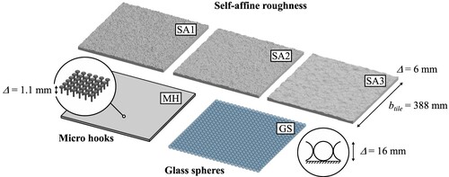
Different types of bed roughness were explored, including (Fig. 1): three types of self-affine (SA) fractal surfaces (Nikora et al., 2019; Stewart et al., 2019), glass spheres (GSs, Cameron et al., 2017) and mushroom-shaped micro hooks (MHs, Zampiron, Nikora, et al., 2020). The three SA roughness patterns feature different scaling exponents $-\text{β}$ of the surface elevation spectra, with $\text{β}=1$ (SA1), $\text{β}=5/3$ (SA2) and $\text{β}=3$ (SA3), having the same roughness height $\Delta =6\text{mm}$, where $\Delta$ is equal to four standard deviations of the bed roughness elevations. The SA roughness was installed in the flume as square periodic tiles with side length $b_{tile}=388\text{mm}$, fully covering the flume bed. The glass spheres had a diameter of $\Delta =16\text{mm}$ and were installed in a hexagonal close packed arrangement, whereas the micro hooks had a height of $\Delta =1.1\text{mm}$ and were installed as a single fabric sheet covering the entire bed of the channel. The SA and the GS roughness types were studied in the AOCF flume, while the MH roughness case was tested in the RS flume.

Figure 1 The bed roughness types considered in this study

The data presented in this paper were collected using PIV and ADV. All flows were uniform (within the fully developed sections of the facilities), turbulent, subcritical and statistically steady. Key hydraulic conditions, the open-channel facility and the measurement technique of the experiments are presented in Table 1. Full sets of hydraulic parameters are provided in the online Supplementary Material (Tables S1–S3).

Table 1 Flow conditions, open-channel facility, and measurement technique used for the experiments

RUN	$H\text{(mm)}$	$u_{\ast }\left(\text{m}{\text{s}}^{-1}\right)$	$U\left(\text{m}{\text{s}}^{-1}\right)$	${\mathsf{R}}_{\mathsf{e}}$ (–)	$\mathsf{F}$ (–)	$B/H$ (–)	$H/\Delta$ (–)	${\Delta }^{+}$ (–)	Technique
SA1_H080*	80	0.024	0.27	21,000	0.30	14.8	13	147	PIV, ADV
SA1_H120*	120	0.024	0.29	35,000	0.27	9.8	20	146	PIV, ADV
SA2_H080*	80	0.024	0.27	21,000	0.30	14.8	13	147	PIV, ADV
SA2_H120*	120	0.024	0.29	35,000	0.27	9.8	20	146	PIV, ADV
SA3_H080*	80	0.024	0.30	24,000	0.34	14.8	13	147	PIV, ADV
SA3_H120*	120	0.024	0.32	39,000	0.30	9.8	20	146	PIV, ADV
GS_H128*	127	0.043	0.49	63,000	0.44	9.3	8	692	PIV
MH_H080**	80	0.029	0.38	30,000	0.43	5.0	73	32	ADV

Note: self-affine roughness $\text{β}=1$ (SA1), $\text{β}=5/3$ (SA2), $\text{β}=3$ (SA3); glass sphere roughness (GS); micro hook roughness (MH); * = AOCF flume; ** = RS flume. Experimental and analysis parameters: $H$ is mean flow depth; $u_{\ast }=\sqrt{gH{S}_b}$ is shear velocity, $g$ is gravity acceleration, $S_b$ is bed slope; $U=Q/\left(BH\right)$ is bulk flow velocity, $Q$ is flowrate, $B$ is channel width; ${\mathsf{R}}_{\mathsf{e}}=UH/\nu$ is bulk Reynolds number, $\nu$ is fluid kinematic viscosity; $\mathsf{F}\mathsf{=}\mathsf{U}\mathsf{/}\sqrt{\mathsf{g}\mathsf{H}}$ is Froude number; $B/H$ is flow aspect ratio; $H/\Delta$ is relative submergence, $\Delta$ is roughness height; and ${\Delta }^{+}=u_{\ast }\Delta /\nu$ is roughness Reynolds number. Please refer to Section 2 for details on the experiments.

Particle image velocimetry (PIV) measurements

In the AOCF with the SA or GS roughness, velocities were measured at different locations in the streamwise direction ($x$) using PIV. The measurement set-ups were different for the two roughness types and are briefly described below. In all cases, the camera configurations allowed measurement of velocities in the region from the roughness tops to the water surface.

For the cases with SA roughness, a stereoscopic four-camera PIV system was used to measure all three velocity components within 225 mm-wide and H-high windows in the y–z plane ($y$ and $z$ are spanwise and vertical coordinates, respectively) with a thickness of ≈ 2 mm in the $x$ direction. The cameras and the laser were installed on a robotic instrumental carriage capable of positioning the PIV measurement window anywhere in the channel. Instrument noise in the second-order velocity statistics was reduced by using the two independent estimates of each velocity component permitted by the four-camera configuration (Cameron et al., 2013). Measurements were made at streamwise spatial increments of $2\times b_{tile}=776\text{mm}$ or $3\times b_{tile}=1164\text{mm}$ depending on the constraints imposed by the external metallic frame of the channel. At each nominal streamwise location, several PIV measurement windows were recorded for the purpose of spatial averaging within domains exceeding the bed roughness scales, while being small compared to the development length of the flow. Two flow conditions for each bed surface (i.e. SA1, SA2, SA3) were studied (Table 1), with flow depths $H\approx 80\text{mm}$ (H080) and $H\approx 120\text{mm}$ (H120), but with the same shear velocity $u_{\ast }=\sqrt{gH{S}_b}\approx 0.024\text{m}{\text{s}}^{-1}$ ($S_b$ is bed slope). The aspect ratios $B/H$ of the flows were 14.8 and 9.8, whereas the relative submergences $H/\Delta$ were ≈ 13 and ≈ 20, respectively. At each streamwise location, velocities were measured for a total of 32 minutes at a sampling rate of 10 Hz. Further details about the experimental set-up and the PIV algorithm can be found in Nikora et al. (2019).

For the GS roughness (run GS_H128, Table 1), a one-camera PIV system was used to measure streamwise and vertical velocity components within 28 windows in the x–z plane with a thickness of ≈ 2 mm (in the $y$ direction), each covering $250\text{mm}\times H$ and spaced at 0.5 m in the streamwise direction. Velocity fields at each streamwise location were measured for 15 min at a sampling rate of 4 Hz. The flow was characterized by a shear velocity $u_{\ast }\approx 0.043\text{m}{\text{s}}^{-1}$ and a flow depth $H\approx 127\text{mm}$, resulting in an aspect ratio $B/H=9.3$ and a relative submergence $H/\Delta \approx 8$ Further information on the experimental set-up can be found in Stewart (2014).

Acoustic Doppler velocimetry (ADV) measurements

Long-duration ADV measurements (Table 1) were carried out in the RS and AOCF flumes at $z/H=0.3$ (with $z=0$ at the mean bed level) at streamwise increments of 1 m. The elevation from the bed was chosen sufficiently high to guarantee an adequate scale separation between LSMs and VLSMs for all cases. The flow in the RS flume over MH roughness (run MH_H080) had a flow depth $H\approx 80\text{mm}$, resulting in an aspect ratio $B/H=5.0$ and a relative submergence $H/\mathrm{\Delta }\approx 73$. The flows over the three SA roughness types in the AOCF had the same nominal hydraulic conditions as in the PIV experiments. In the RS flume, velocity was measured at the centre of the channel with a sampling frequency of 100 Hz for a duration of 8 h ($\approx 136,000H/U$). In the AOCF flume, velocities were measured for 4 h ($\approx 50,000H/U$ for H080 and $\approx 36,000H/U$ for H120) at 100 Hz at two spanwise positions. The first measurement point (P1) was located at the centre of the channel, while the second point (P2) was shifted laterally by $\mathrm{\Delta }y=273\text{mm}$.

2.2 Double averaging and depth averaging

In our assessment of the flow development, we employed double-averaged and depth-averaged flow quantities. An intrinsic double-averaged quantity is defined as a spatial average of a time-averaged quantity $\overline{\zeta }$ (e.g. Nikora et al., 2007): (1) $〈\overline{\zeta }〉(x,y,z)=\frac{1}{\varphi V_0}{\int }_{V_f}\overline{\zeta }(x,y,z)\text{d}V$(1) where the overbar indicates time averaging, the angle brackets indicate spatial averaging, $\text{d}V$ is an infinitesimal volume, $V_f$ is the fluid volume within the total averaging domain of volume $V_0$, and $\varphi =V_f/V_0$ is the roughness geometry function. The spatial averaging domains for our study were selected to be thin slabs parallel to the mean bed with spatial extent well exceeding the scale of bed roughness but being small compared to the scale of the streamwise flow development. For the GS case, the horizontal extent of the averaging domain coincided with the thickness and the streamwise size of the measurement window. For the SA cases, two different domains were employed, both with a streamwise size equal to the thickness of the light sheet, but with different spanwise dimension and location: (i) a b_tile-wide domain located at the centre of the channel used throughout the paper; and (ii) a H-wide domain adjacent to the sidewall used in Section 3.4 only. Double-averaged quantities can be further averaged across the flow depth to obtain depth-averaged quantities (Nikora et al., 2019): (2) $\widehat{〈\overline{\zeta }〉}(x,y)=\frac{1}{H}{\int }_{z_t}^{z_{ws}}\varphi 〈\overline{\zeta }〉(x,y,z)\text{d}z$(2) where the hat symbol is used to indicate depth averaging, $H={\int }_{z_t}^{z_{ws}}\varphi \text{d}z$ is mean flow depth, ${\int }_{z_t}^{z_{ws}}(1-\varphi \text{)d}z$ is mean bed level, $z_t$ is roughness trough elevation, and $z_{ws}$ is water surface elevation. Double-averaged and depth-averaged velocity statistics reported in Section 3 are presented as functions of streamwise coordinate $x$ to assess their evolution along the flow. A right-hand coordinate system with $x_1=x$, $x_2=y$, and $x_3=z$ representing, respectively, the streamwise, transverse and bed normal coordinates, with corresponding velocity components $u_1=u$, $u_2=v$ and $u_3=w$ is used. The origin of $z$ is chosen at the mean bed level, while $x=0$ corresponds to the start of the open-channel section of the flumes, i.e. to the channel entrance.

3 Change of mean velocity and turbulence quantities along the flow

In this section flow development data from the AOCF and the RS flumes are presented.

3.1 Development of vertical profiles of velocity moments

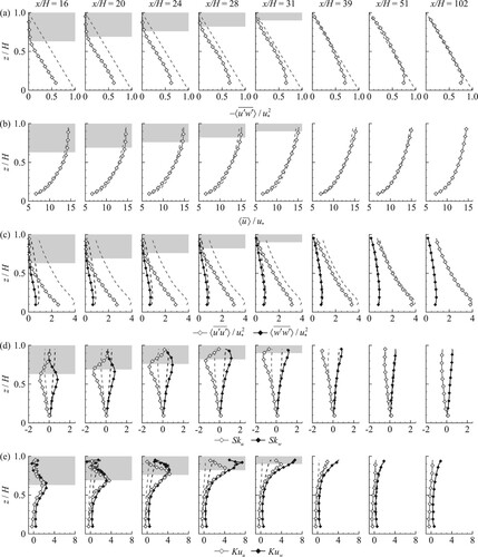
Figure 2 illustrates how vertical distributions of double-averaged velocity statistics (Eq. 1(1) $〈\overline{\zeta }〉(x,y,z)=\frac{1}{\varphi V_0}{\int }_{V_f}\overline{\zeta }(x,y,z)\text{d}V$(1) ), normalized with shear velocity $u_{\ast }=\sqrt{gH{S}_b}$, evolve along the flow. We use the spatially averaged Reynolds stress distribution $-〈\overline{u^{\mathrm{\prime }}{w}^{\mathrm{\prime }}}〉\left(z\right)$ to define the upper edge of the internal boundary layer emerging at the channel entrance. The reason for selecting this approach is because the flow entering the channel does not exhibit noticeable turbulent stresses due to flow conditioning. Thus, the upper edge of the emerging internal boundary layer can be detected as a border between the upper flow region with near-zero stress and the lower region with growing turbulent stress due to boundary layer development. In our study, a threshold value $-〈\overline{u^{\mathrm{\prime }}{w}^{\mathrm{\prime }}}〉/u_{\ast }^2=0.05$, consistent with the approximate uncertainty of the measurements, is adopted for demarcating the upper edge of the internal boundary layer. The flow region above the boundary layer is shaded grey in Fig. 2. The data suggest two distinct stages of the flow development. First, the boundary layer grows in thickness with increasing $x/H$ and covers the entire flow depth by $x/H\approx 40$. Second, statistical distributions of the velocity field continue to evolve and approach their fully developed values between $x/H\approx 50$ and 100. We observe that the interfacial region between the developing boundary layer and the near-free-surface layer is characterized by negative skewness of the streamwise velocity, positive skewness of the vertical velocity and high kurtosis, reflecting intermittent bursts of low momentum fluid originating from the near-bed region being ejected into the outer flow. The streamwise and vertical velocity variance monotonically increase with $x/H$ at all elevations. A qualitatively similar picture is also observed for the other flow cases (not shown here).

Figure 2 Parameters characterizing flow development for run GS_H128. Spatially averaged (a) Reynolds stresses $-〈\overline{u^{\mathrm{\prime }}{w}^{\mathrm{\prime }}}〉/u_{\ast }^2$, (b) mean velocity $〈\overline{u}〉/u_{\ast }$, (c) variance $〈\overline{u^{\mathrm{\prime }}{u}^{\mathrm{\prime }}}〉/u_{\ast }^2$ and $〈\overline{w^{\mathrm{\prime }}{w}^{\mathrm{\prime }}}〉/u_{\ast }^2$, (d) skewness $S{k}_u=〈\overline{u^{\mathrm{\prime }}{u}^{\mathrm{\prime }}{u}^{\mathrm{\prime }}}〉/〈\overline{u^{\mathrm{\prime }}{u}^{\mathrm{\prime }}}{〉}^{1.5}$ and $S{k}_w=〈\overline{w^{\mathrm{\prime }}{w}^{\mathrm{\prime }}{w}^{\mathrm{\prime }}}〉/〈\overline{w^{\mathrm{\prime }}{w}^{\mathrm{\prime }}}{〉}^{1.5}$, and (e) kurtosis $K{u}_u=〈\overline{u^{\mathrm{\prime }}{u}^{\mathrm{\prime }}{u}^{\mathrm{\prime }}{u}^{\mathrm{\prime }}}〉/〈\overline{u^{\mathrm{\prime }}{u}^{\mathrm{\prime }}}{〉}^2-3$ and $K{u}_w=〈\overline{w^{\mathrm{\prime }}{w}^{\mathrm{\prime }}{w}^{\mathrm{\prime }}{w}^{\mathrm{\prime }}}〉/〈\overline{w^{\mathrm{\prime }}{w}^{\mathrm{\prime }}}{〉}^2-3$. Dashed lines in (a) represent the theoretical distribution of fluid shear stress for uniform two-dimensional OCF: $g{S}_b(z_{ws}-z)/u_{\ast }^2$; whereas in (b–e) they show vertical profile of each statistic of the same colour at $x/H=102$ for comparison. Areas in grey denote flow regions above the developing internal boundary layer

3.2 Streamwise evolution of near-surface velocity

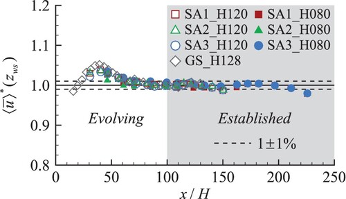
The change of the normalized water surface velocity $〈\overline{u}{〉}^{\ast }\left(z_{ws}\right)$ with $x/H$ is illustrated in Fig. 3, where superscript * denotes normalization with a corresponding value within the fully developed part of the flow (see Section 1.1 for definition). Streamwise velocity distributions were extracted at $z/H\approx 0.95-0.97$, the elevation closest to the water surface at which data were available. The velocity data collapse reasonably well for all cases, indicating that the evolution of $〈\overline{u}〉\left(z_{ws}\right)$ is mostly insensitive to bed roughness type and relative submergence. The streamwise distribution of $〈\overline{u}{〉}^{\ast }\left(z_{ws}\right)$ exhibits a maximum at $x/H\approx 40$, close to the location where the internal boundary layer reaches the water surface, and then $〈\overline{u}{〉}^{\ast }\left(z_{ws}\right)$ gradually decreases and becomes practically constant at $x/H\stackrel{>}{\approx \phantom{{}_2}}80-100$, as highlighted by the grey shaded area in Fig. 3. It should be noted that a similar “velocity overshoot” has been previously observed in pipes (e.g. Bradshaw, 1971; Doherty et al., 2007; Klein, 1981). The increasing free-surface velocity up to $x/H\approx 40$ can be explained by mass conservation and the confining effect of the free surface, while the following reduction of the free-surface velocity reflects continued redistribution of momentum across the flow depth as the turbulence structure evolves and tends to equilibrium. For all cases, we may observe a slight velocity decrease at the last measurement locations, likely caused by the channel exit section.

Figure 3 Streamwise evolution of the normalized double-averaged near-water surface velocity $〈\overline{u}{〉}^{\ast }\left(z_{ws}\right)$. Superscript * denotes normalization on the established velocity values. Areas in grey show the flow region where $〈\overline{u}{〉}^{\ast }\left(z_{ws}\right)$ is within 1 ± 1%

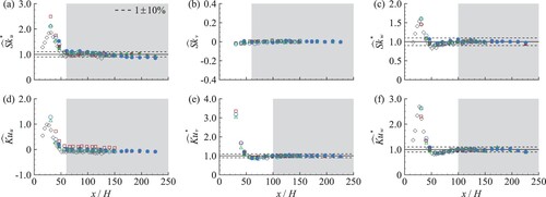
3.3 Development of the turbulence structure

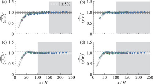
Considering the development of the normalized depth-averaged second-order statistics (Fig. 4), we note that the streamwise variance $〈\stackrel{ˆ}{\overline{u^{\mathrm{\prime }}{u}^{\mathrm{\prime }}}}{〉}^{\ast }$ continues to increase up to $x/H\approx 150$, whereas other stresses ($〈\stackrel{ˆ}{\overline{v^{\mathrm{\prime }}{v}^{\mathrm{\prime }}}}{〉}^{\ast }$, $〈\stackrel{ˆ}{\overline{w^{\mathrm{\prime }}{w}^{\mathrm{\prime }}}}{〉}^{\ast }$, $〈\stackrel{ˆ}{\overline{u^{\mathrm{\prime }}{w}^{\mathrm{\prime }}}}{〉}^{\ast }$) are already fairly well established by $x/H\approx 100$. While the streamwise variance is monotonically increasing throughout, the distributions for $〈\stackrel{ˆ}{\overline{v^{\mathrm{\prime }}{v}^{\mathrm{\prime }}}}{〉}^{\ast }$ and $〈\stackrel{ˆ}{\overline{w^{\mathrm{\prime }}{w}^{\mathrm{\prime }}}}{〉}^{\ast }$ exhibit local maxima at $x/H\approx 60$. Thereafter, $〈\stackrel{ˆ}{\overline{v^{\mathrm{\prime }}{v}^{\mathrm{\prime }}}}{〉}^{\ast }$ and $〈\stackrel{ˆ}{\overline{w^{\mathrm{\prime }}{w}^{\mathrm{\prime }}}}{〉}^{\ast }$ lose around 5% of their energy by $x/H\approx 100$, presumably to the streamwise component.

Figure 4 Streamwise development of the depth-averaged (Eq. 2(2) $\widehat{〈\overline{\zeta }〉}(x,y)=\frac{1}{H}{\int }_{z_t}^{z_{ws}}\varphi 〈\overline{\zeta }〉(x,y,z)\text{d}z$(2) ) velocity (co)variances. Superscript * denotes normalization on the established values. Areas in grey show the flow region where normalized quantities are within 1 ± 5%. Symbols are defined in Fig. 3

The early development of the higher order moments (Figs 2d, e and 5) is dominated by the interfacial region at the upper edge of the boundary layer. This region is characterized by large velocity kurtosis in all components, negative streamwise velocity skewness and positive vertical velocity skewness, reflecting the intermittent upward directed bursts of low momentum fluid from the near bed region. Skewness and kurtosis of the streamwise velocity component and skewness of the spanwise velocity component become essentially established by $x/H\approx 60$, thereafter any trends in the data are indistinguishable from the measurement uncertainty. Skewness and kurtosis of the other velocity components, on the other hand, require development lengths of $x/H\approx 100$ similar to the lower order statistics.

Figure 5 Streamwise development of depth-averaged skewness ${\widehat{Sk}}_{u_i}$ (a–c) and kurtosis ${\widehat{Ku}}_{u_i}$ (d–f). Spatially-averaged skewness and kurtosis were calculated as $S{k}_{u_i}=〈\overline{{u^{\mathrm{\prime }}}_i{u^{\mathrm{\prime }}}_i{u^{\mathrm{\prime }}}_i}〉/〈\overline{{u^{\mathrm{\prime }}}_i{u^{\mathrm{\prime }}}_i}{〉}^{1.5}$ and $K{u}_{u_i}=〈\overline{{u^{\mathrm{\prime }}}_i{u^{\mathrm{\prime }}}_i{u^{\mathrm{\prime }}}_i{u^{\mathrm{\prime }}}_i}〉/〈\overline{{u^{\mathrm{\prime }}}_i{u^{\mathrm{\prime }}}_i}{〉}^2-3$, respectively (no summation over repeated indices), and depth-averaged according to Eq. (2)(2) $\widehat{〈\overline{\zeta }〉}(x,y)=\frac{1}{H}{\int }_{z_t}^{z_{ws}}\varphi 〈\overline{\zeta }〉(x,y,z)\text{d}z$(2) . Superscript * denotes normalization on the established values. No normalization was applied to ${\widehat{Sk}}_v$ and ${\widehat{Ku}}_u$, as their established values were close to zero. Areas in grey show the flow region where normalized quantities are within 1 ± 10%. Symbols are defined in Fig. 3

Development of the streamwise velocity variance is further analysed using pre-multiplied spectra $k_x{F}_{uu}\left(k_x\right)$ in Fig. 6 for the case SA2_H120 (Table 1). The spectra were computed in the frequency domain with 2800 degrees of freedom and transformed to the wavelength domain using ${\lambda }_x=2\pi /k_x=\overline{u}/f$, where $f$ is frequency and $k_x$ is streamwise wavenumber. It is evident from Fig. 6 that larger wavelengths associated with VLSMs develop at a slower rate compared to smaller wavelength structures (LSMs). This trend can also be observed in Fig. 7 where the development of the streamwise component of the turbulent energy associated with LSMs ($H\le {\lambda }_x\le 10H$) is compared to the development of VLSMs (${\lambda }_x>10H$). While LSMs become well established by $x/H\approx 100$ after passing a maximum at $x/H\approx 60$, the energy of VLSMs continues to generally increase up to $x/H\approx 150$.

Figure 6 Pre-multiplied spectra of streamwise velocity measured at $z/H=0.3$ in P1 (see section 2.1) for run SA2_H120 (flow over self-affine roughness with $\text{β}=5/3$). Spectra are shown for selected measurement streamwise location for clarity. Symbols denote different streamwise locations. Vertical dashed line at ${\lambda }_x/H=10$ represents an approximate border separating the dominant contributions from LSMs and VLSMs

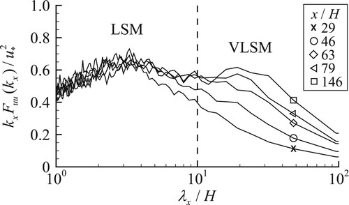
Figure 7 Streamwise velocity variance associated with (a) LSMs (${\overline{u^{\mathrm{\prime }}{u}^{\mathrm{\prime }}}}_{LSM}$) and (b) VLSMs (${\overline{u^{\mathrm{\prime }}{u}^{\mathrm{\prime }}}}_{VLSM}$). Superscript * denotes normalization on the established values. Areas in grey denote the region of flow where normalized quantities are within 1 ± 10%. In the SA runs, symbols with black “/” represent measurements at P1, whereas symbols without represent measurements at P2 (see Section 2.1 and Fig. 8 for location of P1 and P2)

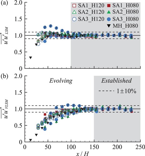
Figure 8 Velocity distribution across the channel. (a) spatial-averaging domains, (b) distributions of time-averaged velocities at different streamwise locations for SA3_H120. In (b), vectors represent spanwise ($\overline{v}/U$) and vertical ($\overline{w}/U$) time-averaged velocities, dash-dotted lines mark channel centreline at $y=590\text{mm}$, and “×” and “+” symbols show P1 and P2 (see Section 2.1), respectively

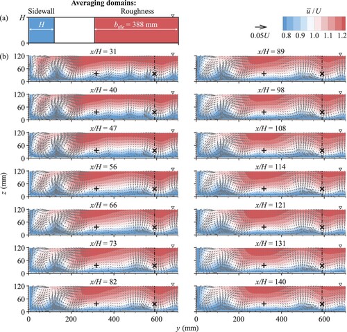
3.4 Development of secondary currents

Figure 8b shows how the time-averaged velocity field develops for the case SA3_H120. Much of the flow is occupied by SCs, appearing as time-averaged streamwise vortices (e.g. Nezu & Nakagawa, 1993). We may distinguish two types of SCs in a straight channel: (i) sidewall SCs which typically decay within a few flow depths from the sidewalls, and (ii) SCs tied to the spanwise roughness variation (in our study of SA roughness this variation was introduced by the repetitive effect of the selected roughness elements, as identical roughness tiles followed each other in the streamwise direction over the whole flume length; Nikora et al., 2019). The noticeable flow asymmetry in respect to the channel centreline is associated with the presence of roughness-induced SCs. The strength of the SCs may be characterized by the depth-averaged dispersive stresses $〈\stackrel{ˆ}{{\tilde{\overline{u}}}_i{\tilde{\overline{u}}}_j}〉$, where the spatial fluctuation ${\tilde{\overline{u}}}_i$ of the ith time-averaged velocity component is calculated as ${\tilde{\overline{u}}}_i={\overline{u}}_i-〈{\overline{u}}_i〉$. We employ two spatial-averaging domains to capture sidewall and roughness-induced SCs independently (Section 2.2). In each case, the domain was a thin slab (≈ 2 mm thick) parallel to the mean bed and extended laterally across the flow regions illustrated in Fig. 8a. Subsequent depth averaging (Eq. 2) of the dispersive stress distributions resulted in the data presented in Fig. 9.

Figure 9 Streamwise change of the depth-averaged (Eq. 2(2) $\widehat{〈\overline{\zeta }〉}(x,y)=\frac{1}{H}{\int }_{z_t}^{z_{ws}}\varphi 〈\overline{\zeta }〉(x,y,z)\text{d}z$(2) ) dispersive stress components computed within (left column) “sidewall” and (right column) “roughness” averaging domains defined in Fig. 8a. Superscript * denotes normalization on the established values. Areas in grey show the region of flow where normalized quantities are within 1 ± 10%. Symbols are defined in Fig. 7

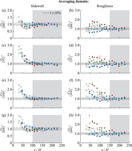
The sidewall SCs continue to develop until around $x/H\approx 100$ and then almost stabilize, although some minor change might still be observed downstream, probably due to the interaction with the roughness-induced SCs and the VLSMs. The data in Fig. 9 suggest that the sidewall SCs grow quickly and reach the maximum strength somewhere within $x/H<30$, where data are not available. The roughness generated SCs, in comparison, exhibit a less clear trend, with the distributions highly dependent on the flow condition and roughness type. In some cases, the strength of the roughness-induced SCs continues to develop up to $x/H\approx 150$, potentially reflecting some interaction with VLSMs which were seen to become fully established at a similar streamwise coordinate. This trend, however, may not be typical and the situation with other forms of roughness spanwise heterogeneity, such as continuous streamwise ridges (Zampiron, Cameron, et al., 2020, 2021), may be different.

5 Conclusions

In this work, we studied the development of OCFs for a range of bed roughness and hydraulic conditions. The change in mean flow and turbulence statistics along the streamwise coordinate was explored using PIV and ADV measurements in two open-channel flumes. The data suggest that the flow development can be divided into two main stages: (i) the initial part of the channel starting from the flume entrance where an internal boundary layer grows in thickness and covers the entire flow depth by around $x\approx 40H$, and (ii) a subsequent part of the channel where mean flow and most conventional turbulence statistics continue to develop, reaching a fully developed condition by around $x\approx 100H$. However, streamwise velocity variance, VLSMs and roughness-induced SCs, if present, may require even longer development lengths approaching $150H$. The first stage of flow development is characterized by rapid changes in mean velocity and velocity variance, while depth-averaged velocity skewness and kurtosis are strongly affected by an interfacial region separating the boundary layer and the near surface flow. The internal boundary layer reaches the free surface at $x\approx 40H$ where this location coincides with a local maximum in the free surface velocity which emerges due to mass conservation and the confining effect of the free surface. Flow development in the second stage is more gradual as mean velocity, velocity variance and higher order moments asymptotically approach their fully developed values.

With exception of the roughness-induced SCs, the data presented in this study suggest a dependency of the flow development on the normalized streamwise coordinate $x/H$ only. Indeed, while a substantial effect of ${\mathsf{R}}_{\mathsf{e}}$, ${\mathrm{\Delta }}^{+}$, $\mathsf{F}$ and $B/H$ was not expected (i.e. the flows were fully turbulent, rough, subcritical and wide), no measurable effect of $H/\Delta$ or roughness type was observed either, despite the significant differences between the studied types of bed roughness. On the other hand, the development of roughness-induced SCs seemed the result of an interplay between different flow parameters (e.g. ${\mathsf{R}}_{\mathsf{e}}$, $B/H$, $H/\Delta$ and bed roughness characteristics) and needs to be further explored.

Our results suggest that caution should be applied in interpreting distributions of mean velocities and turbulence parameters reported in the literature, as many studies do not provide sufficient details on the measurement location, or they present data measured at streamwise distances from the flume entrance substantially smaller than $100H$. As a rule of thumb, we propose that for uniform OCFs the experimental designs should involve turbulence measurements at distances from the channel entrance of around $100H$ or larger. This value significantly exceeds the $40-50H$ typically assumed based on the previous works (see references in Section 1.2). Note that even longer distances may be required in the case undesired patterns are introduced in the incoming flow by unfavourable entrance conditions. The scaling for the flow development length for non-uniform OCFs is currently unknown and requires a special study.

Notation

$B$	=	channel width (m)
$f$	=	frequency (Hz)
$\mathsf{F}$	=	Froude number (–)
$F_{uu}$	=	spectral magnitude of streamwise velocity (m3 s−2)
$g$	=	gravity acceleration (m s−2)
$H$	=	mean flow depth (m)
$k_x$	=	streamwise wavenumber $\left(\mathrm{r}\mathrm{a}\mathrm{d}{\mathrm{m}}^{-1}\right)$
$L_D$	=	flow development length (m)
${\mathsf{R}}_{\mathsf{e}}$	=	Reynolds number (–)
$S_b$	=	channel bed slope (–)
$u$	=	streamwise velocity component (m s−1)
$u_{\ast }$	=	shear velocity (m s−1)
$U$	=	flow bulk velocity (m s−1)
$v$	=	spanwise velocity component (m s−1)
$w$	=	vertical velocity component (m s−1)
$x$	=	streamwise coordinate (–)
$y$	=	spanwise coordinate (–)
$z$	=	vertical coordinate (–)
$z_t$	=	roughness trough elevation (m)
$z_{ws}$	=	water surface elevation (m)
$\Delta$	=	roughness height (m)
${\lambda }_x$	=	streamwise wavelength (m)
$\nu$	=	kinematic viscosity of the fluid (m2 s−1)
$\varphi$	=	roughness geometry function (–)

Acknowledgements

The authors wish to express their gratitude to Roy Gillanders for the help provided in the laboratory and to the School of Engineering of the University of Aberdeen for the support. The comments and suggestions of the Associate Editor and two anonymous reviewers helped to improve the final version of the paper and are much appreciated.

Disclosure statement

No potential conflict of interest was reported by the authors.

Supplemental data

Supplemental data for this article can be accessed at http://dx.doi.org/10.1080/00221686.2022.2132311.

Correction Statement

This article was originally published with errors, which have now been corrected in the online version. Please see Correction (http://doi.org/10.1080/00221686.2023.2292906)

Additional information

Funding

The study has been supported by three Engineering and Physical Sciences Research Council/UK grants: “High-resolution numerical and experimental studies of turbulence-induced sediment erosion and near-bed transport” (EP/G056404/1), “Bed friction in rough-bed free-surface flows: a theoretical framework, roughness regimes, and quantification” (EP/K041088/1) and “Secondary currents in turbulent flows over rough walls” (EP/V002414/1).

References

- Barbin, A. R., & Jones, J. B. (1963). Turbulent flow in the inlet region of a smooth pipe. Journal of Basic Engineering, 85(1), 29–33. http://doi.org/10.1115/1.3656521
- Bradshaw, P. (1971). An introduction to turbulence and its measurement. Pergamon Press.
- Cameron, S. M., Nikora, V. I., Albayrak, I., Miler, O., Stewart, M., & Siniscalchi, F. (2013). Interactions between aquatic plants and turbulent flow: A field study using stereoscopic PIV. Journal of Fluid Mechanics, 732, 345–372. http://doi.org/10.1017/jfm.2013.406
- Cameron, S. M., Nikora, V. I., & Stewart, M. T. (2017). Very-large-scale motions in rough-bed open-channel flow. Journal of Fluid Mechanics, 814, 416–429. http://doi.org/10.1017/jfm.2017.24
- Das, S., Balachandar, R., & Barron, R. M. (2022). Generation and characterization of fully developed state in open channel flow. Journal of Fluid Mechanics, 934, A35. http://doi.org/10.1017/jfm.2021.1133
- Demuren, A. O., & Rodi, W. (1984). Calculation of turbulence-driven secondary motion in non-circular ducts. Journal of Fluid Mechanics, 140, 189–222. http://doi.org/10.1017/S0022112084000574
- Doherty, J., Ngan, P., Monty, J., & Chong, M. (2007). The development of turbulent pipe flow. 16th Australasian Fluid Mechanics Conference, Brisbane, Australia, 266–270.
- Graf, W. H., & Altinakar, M. S. (1998). Fluvial hydraulics. John Wiley & Sons.
- Kim, K. C., & Adrian, R. J. (1999). Very large-scale motion in the outer layer. Physics of Fluids, 11(2), 417–422. http://doi.org/10.1063/1.869889
- Kirkgo¨z, M. S., & Ardiçlioğlu, M. (1997). Velocity profiles of developing and developed open channel flow. Journal of Hydraulic Engineering, 123(12), 1099–1105. http://doi.org/10.1061/(ASCE)0733-9429(1997)123:12(1099)
- Klein, A. (1981). Review: Turbulent developing pipe flow. Journal of Fluids Engineering, 103(2), 243–249. http://doi.org/10.1115/1.3241726
- Marusic, I., Chauhan, K. A., Kulandaivelu, V., & Hutchins, N. (2015). Evolution of zero-pressure-gradient boundary layers from different tripping conditions. Journal of Fluid Mechanics, 783, 379–411. http://doi.org/10.1017/jfm.2015.556
- Monin, A. S., & Yaglom, A. M. (1971). Statistical fluid mechanics, volume I: Mechanics of turbulence. MIT press.
- Nezu, I., & Nakagawa, H. (1993). Turbulence in open-channels flows. Balkema.
- Nikora, V., McEwan, I., McLean, S., Coleman, S., Pokrajac, D., & Walters, R. (2007). Double-averaging concept for rough-bed open-channel and overland flows: Theoretical background. Journal of Hydraulic Engineering, 133(8), 873–883. http://doi.org/10.1061/(ASCE)0733-9429(2007)133:8(873)
- Nikora, V. I., Goring, D. G., & Biggs, B. J. F. (1998). Silverstream eco-hydraulics flume: Hydraulic design and tests. New Zealand Journal of Marine and Freshwater Research, 32(4), 607–620. http://doi.org/10.1080/00288330.1998.9516848
- Nikora, V. I., Stoesser, T., Cameron, S. M., Stewart, M., Papadopoulos, K., Ouro, P., McSherry, R., Zampiron, A., Marusic, I., & Falconer, R. A. (2019). Friction factor decomposition for rough-wall flows: Theoretical background and application to open-channel flows. Journal of Fluid Mechanics, 872, 626–664. http://doi.org/10.1017/jfm.2019.344
- Ranga Raju, K. G., Asawa, G. L., & Mishra, H. K. (2000). Flow-establishment length in rectangular channels and ducts. Journal of Hydraulic Engineering, 126(7), 533–539. http://doi.org/10.1061/(ASCE)0733-9429(2000)126:7(533)
- Reichert, J. K., & Azad, R. S. (1976). Nonasymptotic behavior of developing turbulent pipe flow. Canadian Journal of Physics, 54(3), 268–278. http://doi.org/10.1139/p76-032
- Schlichting, H. (1979). Boundary-layer theory. McGraw-Hill, Inc.
- Stewart, M. T. (2014). Turbulence structure in rough-bed open-channel flow [Doctoral thesis]. University of Aberdeen.
- Stewart, M. T., Cameron, S. M., Nikora, V. I., Zampiron, A., & Marusic, I. (2019). Hydraulic resistance in open-channel flows over self-affine rough beds. Journal of Hydraulic Research, 57(2), 183–196. http://doi.org/10.1080/00221686.2018.1473296
- Townsend, A. A. (1976). The structure of turbulent shear flow. Cambridge University Press.
- Wilkerson, G., Sharma, S., & Sapkota, D. (2019). Length for uniform flow development in a rough laboratory flume. Journal of Hydraulic Engineering, 145(1), 06018018. http://doi.org/10.1061/(ASCE)HY.1943-7900.0001554
- Yalin, M. S. (1977). Mechanics of sediment transport (2nd ed.). Pergamon Press.
- Zampiron, A., Cameron, S., & Nikora, V. (2020). Secondary currents and very-large-scale motions in open-channel flows over streamwise ridges. Journal of Fluid Mechanics, 887(1). http://doi.org/10.1017/jfm.2020.8
- Zampiron, A., Cameron, S., & Nikora, V. (2021). Momentum and energy transfer in open-channel flow over streamwise ridges. Journal of Fluid Mechanics, 915, A42. http://doi.org/10.1017/jfm.2021.44
- Zampiron, A., Nikora, V., Cameron, S., Patella, W., Valentini, I., & Stewart, M. (2020). Effects of streamwise ridges on hydraulic resistance in open-channel flows. Journal of Hydraulic Engineering, 146(1), 06019018. http://doi.org/10.1061/(ASCE)HY.1943-7900.0001647