General shallow water equations (GSWEs)

Abstract

Shallow water equations (SWEs) have been traditionally derived by integrating fundamental flow equations over a flow profile above a single point in a horizontal or nearly horizontal plane, with the main assumptions that the profile thickness is much smaller than other two dimensions and it contains only water. This paper presents the derivation of generalized SWEs (GSWEs) obtained for a finite plan area, allowing for the presence of phases other than water, such as air, grains, vegetation, and debris, which can be either stationary or mobile. The derivation provides a rigorous basis for various applications of layer-averaged models and opens numerous research questions, some of which are highlighted in the paper.

Keywords:

• Aerated flows
• bed-load
• debris flows
• rough bed
• SWEs
• vegetated channel

1. Introduction

The shallow water equations (SWEs) are a well-known classical mathematical framework for describing flow in a thin layer of fluid. They are able to describe many different types of flows ranging from tsunami waves (e.g. Wang et al., 2021; Wuppukondur & Baldock, 2022) and waves on shallow beaches (e.g. Hibberd & Peregrine, 1979; Hubbard & Dodd, 2000) to flood waves in rivers (e.g. Ayog et al., 2021; Yu & Chang, 2021) and urban areas (e.g. Dong et al., 2021; Li et al., 2020). Despite “Water” in their name the SWEs are also used for describing gravity currents (e.g. Adduce et al., 2012; Ungarish, 2007), dry avalanches (e.g. Savage & Hutter, 1989), debris flow (Xiong et al., 2020), and even magnetohydrodynamics (e.g. Lahaye & Zeitlin, 2022). The common feature of all these diverse kinds of flow is that they can be considered as shallow, because they occur in a layer with a much smaller thickness and the corresponding layer-normal velocity than the length and velocity scales in the layer-parallel directions.

The derivation of SWEs can be found in many classical textbooks and papers (Peregrine, 1972; Stoker, 1957; Toro, 2001; Whitham, 1974 to name just a few). The derivation is carried out by depth-integrating the 3D fundamental volume and momentum balance equations (either Navier–Stokes or Reynolds-averaged Navier–Stokes equations), and assuming hydrostatic pressure distribution. The resulting 2D or 1D flow description provides the basis for computationally efficient numerical simulation codes, making the SWE-based models very attractive for practical engineering models (e.g. ANUGA, Roberts et al., 2009, BASEMENT, Volz et al., 2012, LISFLOOD-FP, Neal et al., 2012).

Besides the main assumption of shallow flow, the original derivation of the SWEs involves a few more assumptions: the flow layer contains only one fluid, usually water, the free surface does not fluctuate around its relatively slowly moving position, and all forces other than pressure (and gravity for non-horizontal flows) are negligible. The SWEs are then derived by integrating the fundamental flow equations over a single flow profile, between the bed and the free-surface level.

For the purpose of expanding their applicability, the original SWEs have been modified by including the effects that were deemed important such as turbulent stress, the bed shear stress at the bottom boundary (e.g. Stansby & Feng, 2005) and other effects. There is clearly a desire to expand the application of the SWEs beyond the modelling of clear water flow. Examples of such models are hydro-sediment morphodynamics models (e.g. Carraroa et al., 2018). However, the depth-averaged equations needed for such models are usually developed by integration over a single flow profile located at a point in the plan area. Such an approach is not suitable for rigorous definitions of the terms that arise for flow over a finite plan area that covers a representative sample of the bed geometry, for instance bed shear stress which results from forces acting on the bed across the entire finite area. Such terms are instead added intuitively (e.g. Ayog et al., 2021; Mignot et al., 2006 and numerous other papers) – a quick and simple approach, but lacking clarity and rigour. This gap in knowledge has motivated the author to revisit the derivation of the SWEs, remove all assumptions other than that of shallow flow, and carry out the derivation which considers flow over a finite plan area rather than over a point. The derivation has been performed using the already existing generalized double averaging methodology (V. Nikora et al., 2013), with slightly modified notation which allows for a clear distinction between the two averaging steps and a rigorous definition of intrinsic averages. It has yielded a general version of the traditional SWEs. The new equations will be referred to as GSWEs with “G” standing for “Generalized”.

The derivation is presented for a single layer which contains mainly water, but can also include air bubbles, stationary and moving grains, vegetation, and other solid objects. The same methodology can be used to derive underlying equations for various multi-layer models.

The paper is organized as follows. The next section provides a brief overview of the main concepts and definitions (the details are presented in the appendices). It also describes the physical system to which the GSWEs apply, and the additions to the classical double-averaging methodology needed for its application for deriving the GSWEs. Sections 3 and 4 summarize the derivation of the continuity and momentum GSWEs, respectively. Section 5 highlights some open research questions and directions related to the derived GSWEs. The final section contains few concluding remarks.

2. Main concepts and definitions

The derivation of the GSWEs presented in this paper can be considered as an extended version of the derivation of classical SWEs'. While classical SWEs are derived by averaging over a single flow profile/water column located at a point in the plan area, the GSWEs will be derived by averaging over all flow profiles covering a finite plan area. This is necessary for flows over rough beds, those with irregular free surface, and those containing phases other than water in the water column because for such cases the finite plan area needs to capture representative samples of the bed, the free surface, and phases other than water. The extension from SWEs to GSWEs therefore involves expanding the bottom and the top boundaries of the water column from points into surfaces, and the use of the spatial averaging theorems instead of the Leibniz integral rules: the theorems contain the terms which express the conditions along the bottom and the top surfaces that correspond to the terms in the Leibniz rules expressing the conditions at the bottom and top points. In either case the derivation transforms the original 3D description/model of the problem to 2D depth-averaged description, so that the bottom and top boundary conditions of the 3D model become source terms in the 2D model.

Besides spatial averaging needed to capture flow heterogeneity due to the presence of small-scale features, time averaging is needed to account for turbulence effects. This makes the double averaging methodology a convenient theoretical framework for deriving GSWEs.

2.1. Averaging approach

Double averaging methodology in its classical form (e.g. Finnigan, 2000; V. I. Nikora et al., 2001; Wilson & Shaw, 1977) involves two averaging steps, one over a time interval (or over an ensemble of statistical realizations), and another one over a volume. In order to incorporate turbulent quantities defined in classical way the time averaging step is usually performed first, but reversing the order may be conceptually simpler (Pokrajac & Kikkert, 2011). It is also possible to perform the two averaging steps simultaneously (V. Nikora et al., 2013).

In order to produce large-scale equations which include classical turbulent quantities and hence build on the wealth of knowledge on turbulence, this paper presents the large-scale equations derived using two averaging steps, i.e. either time/ensemble averaging followed by spatial averaging or vice-versa. Deriving large-space equations using simultaneous time/space averaging is analogous and simpler in mathematical terms, so it will not be further considered.

The derivations are carried out for a general case which allows for a possibility to have gaps (points not occupied by the fluid) in both spatial and temporal domains. Such gaps occur, for instance, over the volumes of individual solid grains, or at locations close to the water surface at time instances when they are dry. The large-scale equations for this general case have been derived in V. Nikora et al. (2013), where they have been applied to a thin bed parallel averaging volume, which covers a sufficiently large plan area. In this paper the identical methodology is applied to a “thick” averaging volume which covers the entire flow depth.

All definitions of averaging operators and relevant quantities and rules are provided in Appendix A, and only the key relationships needed for the derivation of the GSWEs are repeated here. The notation used to denote temporal and spatial averages (overbar and square brackets for time and space averages, respectively) and related quantities is the same as in the most of the DAM literature, with the following amendment. For the purpose of having precise definitions it is beneficial to distinguish between the first and the second averaging step, so the former is highlighted by adding a symbol ° (standing for “one”) to all operators applied and quantities obtained in the first averaging step.

For both time and volume averaging the term “superficial average” refers to the average carried over the entire averaging window (see Eqs A1(A1) $\begin{array}{rl}& {\overline{\theta }}^{s\circ }\left(x_i\right)=\frac{1}{T_0}{\int }_{T_0}\theta (x_i,t)\gamma (x_i,t)\mathrm{d}t,\\ & {〈\theta 〉}^{s\circ }\left(t\right)=\frac{1}{V_0}{\int }_{V_0}\theta (x_i,t)\gamma (x_i,t)\mathrm{d}V\end{array}$(A1) and A5(A5) $\begin{array}{rl}& {〈\psi 〉}^s=\frac{1}{V_0}{\int }_{V_0}\psi \left(x_i\right){\overline{\gamma }}^{\circ }\left(x_i\right)\mathrm{d}V,\\ & {\overline{\phi }}^s=\frac{1}{T_0}{\int }_{T_0}\phi \left(t\right){〈\gamma 〉}^{\circ }\left(t\right)\mathrm{d}t\end{array}$(A5) for definitions), whereas “intrinsic average” indicates averaging over the part of the averaging window occupied by the main fluid (Eqs A2 and A7(A7) $\begin{array}{rl}& 〈\psi 〉=\frac{1}{V_f}{\int }_{V_0}\psi \left(x_i\right){\overline{\gamma }}^{\circ }\left(x_i\right)\mathrm{d}V,\\ & \overline{\phi }=\frac{1}{T_f}{\int }_{T_0}\phi \left(t\right){〈\gamma 〉}^{\circ }\left(t\right)\mathrm{d}t\end{array}$(A7) ). These parts are tracked using a “marker function” $\gamma (x_i,t)$ which takes the value of one if the fluid occupies the point $x_i$ at time t, and the value of zero otherwise (Fig. A1b). The ratios of the parts of averaging windows that contain the main fluid and the entire averaging windows, called “space and time porosity” in V. Nikora et al. (2013), are here referred to as spatial and temporal “occupancy ratios”. They provide the relationships between superficial and intrinsic averages of a generic fluid quantity θ, which are derived in Appendix A (Eqs A4, A8(A8) $\begin{array}{rl}{〈\psi 〉}^s& ={\varphi }_{{}_V}〈\psi 〉,\\ {\overline{\phi }}^s& ={\varphi }_{{}_T}\overline{\phi }\end{array}$(A8) ) and repeated here for convenience: (1) $\begin{array}{r}\begin{array}{rlrl}{\overline{\theta }}^{s\circ }& ={\varphi }_{{}_T}^{\circ }{\overline{\theta }}^{\circ },& {〈\theta 〉}^{s\circ }& ={\varphi }_{{}_V}^{\circ }{〈\theta 〉}^{\circ },\\ {〈\psi 〉}^s& ={\varphi }_{{}_V}〈\psi 〉,& {\overline{\phi }}^s& ={\varphi }_{{}_T}\overline{\phi }\end{array}\end{array}$(1) The first and the second rows of Eq. (1(1) $\begin{array}{r}\begin{array}{rlrl}{\overline{\theta }}^{s\circ }& ={\varphi }_{{}_T}^{\circ }{\overline{\theta }}^{\circ },& {〈\theta 〉}^{s\circ }& ={\varphi }_{{}_V}^{\circ }{〈\theta 〉}^{\circ },\\ {〈\psi 〉}^s& ={\varphi }_{{}_V}〈\psi 〉,& {\overline{\phi }}^s& ={\varphi }_{{}_T}\overline{\phi }\end{array}\end{array}$(1) ) are for the first and second averaging step, respectively. The second averaging step is performed over the results of the first step, which are denoted as ψ and φ: $\psi \left(x_i\right)$ denotes a result of the first averaging step over time, i.e. either ${\overline{\theta }}^{s\circ }$ or ${\overline{\theta }}^{\circ }$, or any other function with the same marker function ${\overline{\gamma }}^{\circ }\left(x_i\right)$, for instance ${\varphi }_{{}_T}^{\circ }$, see Fig. A2; $\phi \left(t\right)$ is a first step volume average (${〈\theta 〉}^{s\circ }$, or ${〈\theta 〉}^{\circ }$), or any other function marked by ${〈\gamma 〉}^{\circ }\left(t\right)$, such as ${\varphi }_{{}_V}^{\circ }$. These relationships have been defined in V. Nikora et al. (2013), where ${\varphi }_{{}_V}$ and ${\varphi }_{{}_T}$ were denoted with ${\varphi }_{{}_{V_m}}$ and ${\varphi }_{{}_{T_m}}$, respectively.

Figure 1. The averaging volume, $V_0$, covers a section of an open channel between dark grey lines. (a) The content of the averaging volume at an arbitrary time instant: water (light grey), air (white), grains and other solid objects such as debris and vegetation (dark grey if immobile and textured if mobile). Velocities of mobile objects are shown with arrows. Thick red lines indicate the bottom and the top boundaries, denoted with $BOT,TOP$ respectively, which are the conceptual interfaces of the 2D model with the adjacent layers. The right-handed main coordinate system x, y, z has inclination angles relative to the horizontal plane ${\alpha }_x$ and ${\alpha }_y$. Another Cartesian coordinate system has the $x_{bed},y_{bed}$ plane aligned with the average bed plane, and the inclination angles relative to the xy plane ${\text{β}}_x$ and ${\text{β}}_y$. (b) The averaging volume shown in (a) prepared for spatial averaging: water is light grey and its interfaces with other fluid phases or objects are shown as thick black or blue lines. Black lines indicate the interfaces associated with either top or the bottom boundary, and blue lines show those within the water column. Thick red lines show the wet parts of either bottom or top boundary which, for the purpose of deriving GSWEs, also act as interfaces because water located beyond them (above the top and below the bottom boundary) has been deleted. The black and the red interfaces along the bottom and the top boundaries joined together form the bottom and the top surfaces denoted with $S_{bot},S_{top}$ respectively. Geometry of all interfaces is defined by a unit normal vector $\overrightarrow{n}$ pointing into water

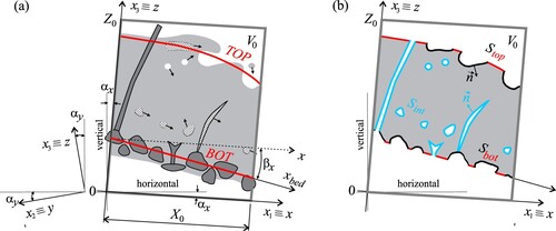
After each averaging step the intrinsic averages resulting from it can be used to decompose the variable that has been averaged into an intrinsic average and the deviation from this average. The deviations are denoted with a prime and a tilde for a deviation from the temporal and spatial intrinsic average, respectively. The usual rules, e.g. of sum and product, apply for the intrinsic averages of two or more variables (Eq. A9(A9) $\begin{array}{rl}{\overline{{\theta }_1+{\theta }_2}}^{\circ }& ={\overline{{\theta }_1}}^{\circ }+{\overline{{\theta }_2}}^{\circ },\\ {\overline{{\theta }_1{\theta }_2}}^{\circ }& ={\overline{{\theta }_1}}^{\circ }{\overline{{\theta }_2}}^{\circ }+{\overline{{{\theta }_1}^{\mathrm{\prime }\circ }{{\theta }_2}^{\mathrm{\prime }\circ }}}^{\circ },\\ 〈{\psi }_1+{\psi }_2〉& =〈{\psi }_1〉+〈{\psi }_2〉,\\ 〈{\psi }_1{\psi }_2〉& =〈{\psi }_1〉〈{\psi }_2〉+〈\widetilde{{\psi }_1}\widetilde{{\psi }_2}〉\end{array}$(A9) ).

The superficial averages applied in the two consecutive steps commute, i.e. reversing their order produces identical result. The relationships between superficial and intrinsic double averages developed in Appendix B (Eq. B2(B2) $\begin{array}{rl}{〈{\overline{\theta }}^{s\circ }〉}^s& ={\varphi }_{{}_V}〈{\varphi }_{{}_T}^{\circ }{\overline{\theta }}^{\circ }〉\\ & ={\varphi }_{{}_V}〈{\varphi }_{{}_T}^{\circ }〉〈{\overline{\theta }}^{\circ }〉+{\varphi }_{{}_V}〈\widetilde{{\varphi }_{{}_T}^{\circ }}\widetilde{{\overline{\theta }}^{\circ }}〉={〈{\varphi }_{{}_T}^{\circ }〉}^s〈{\overline{\theta }}^{\circ }〉+{〈\widetilde{{\varphi }_{{}_T}^{\circ }}\widetilde{{\overline{\theta }}^{\circ }}〉}^s,\\ {\overline{{〈\theta 〉}^{s\circ }}}^s& ={\varphi }_{{}_T}\overline{{\varphi }_{{}_V}^{\circ }{〈\theta 〉}^{\circ }}={\varphi }_{{}_T}\overline{{\varphi }_{{}_V}^{\circ }}\overline{{〈\theta 〉}^{\circ }}+{\varphi }_{{}_T}\overline{{\varphi }_{{}_V}^{{\circ }^{\prime }}{〈\theta 〉}^{{\circ }^{\prime }}}\\ & ={\overline{{\varphi }_{{}_V}^{\circ }}}^s\overline{{〈\theta 〉}^{\circ }}+{\overline{{\varphi }_{{}_V}^{{\circ }^{\prime }}{〈\theta 〉}^{{\circ }^{\prime }}}}^s\end{array}$(B2) ) show that intrinsic averages do not commute in a general case analysed in this paper, but do commute in the following special cases: (i) neither ${\varphi }_{{}_T}^{\circ }$ and ${\overline{\theta }}^{\circ }$, nor ${\varphi }_{{}_V}^{\circ }$ and ${〈\theta 〉}^{\circ }$ are correlated; (ii) all interfaces between the main fluid and other phases are “frozen”, i.e. immobile.

2.2. Basic concepts relevant for derivations of the GSWEs

Figure 1a shows a sketch of a possible general case for which the GSWEs will be derived, with a snapshot of all phases at an arbitrary time instant. The main fluid is water, which flows over a permeable bed made of stationary grains, and carries mobile objects such as sediment grains and debris. There is also aquatic vegetation, which may be either immobile or mobile. The free surface is irregular, and the water column may contain air bubbles.

The Cartesian right-handed coordinate system is used throughout the paper, with either tensorial ($x_i,i=1,2,3$) or hydraulic (x, y, z) notation. In the former case Einstein summation convention applies. The streamwise and lateral coordinates $x_1\equiv x$ and $x_2\equiv y$ follow the two principal directions of the double-averaged flow. Their inclination angles relative to the horizontal plane are denoted with ${\alpha }_x$, and ${\alpha }_y$, respectively. More precisely, rotation of the x, y, z system about the y axis by ${\alpha }_x$ brings the x axis into the horizontal plane, and another rotation (about the new position of x) by ${\alpha }_y$ brings the y axis into the horizontal plane and hence also makes the z axis vertical. The velocity components corresponding to the coordinate axes are $u_1\equiv u,u_2\equiv v,u_3\equiv w$ respectively.

The averaging volume is shown with thick dark grey lines in Fig. 1. It is a cuboid with a base in the x, y plane (i.e. at z = 0), centred at an arbitrary $(x,y)$ point. Its dimensions in the three coordinate directions are $X_0,Y_0,Z_0$. Geometry of all interfaces between water and other phases is defined by their outer unit normal vectors, $n_i$, pointing into water (Fig. 1b). The classical requirement for volume averaging to produce physically meaningful results is that it is done over the so-called representative elementary volume (REV) (Bear, 1972). REV is a volume which is sufficiently large to provide stable averaging results and sufficiently small to avoid large (macroscopic) scale effects. For the general case considered here the volume should be sufficiently large to provide a statistically representative sample of all phases, i.e. grains, vegetation, any other solid objects, and air bubbles, and sufficiently small to avoid smoothing larger structures, for instance bed forms. An analogous requirement for time averaging is that there is a clear separation of scales between the rapid changes within the time-averaging window, and the slow variation of the time-averaged quantities. The practical implications of these requirements depend on the scales of interest for a particular problem. For some practical problems it may be impossible to strictly satisfy either of these requirements, for instance the separation of time scales of turbulence and bulk flow unsteadiness. It may still be possible to use the derived GSWEs as a framework, and to account for the effect of the overlapping scales by adjusting the turbulence closure models, e.g. Zilitinkevich et al. (2009).

The thick red lines in Fig. 1a show the lower and the upper boundaries of the flow layer, BOT and TOP, with their respective z coordinates denoted with $z_{{}_{BOT}}$ and $z_{{}_{TOP}}$. They are fictive boundaries introduced in the original 3D problem description to define the boundaries of integration required for transition from 3D to 2D description. This transition will convert the boundary conditions acting along the boundaries into source terms in 2D equations in a manner analogous to the derivation of the classical SWEs, where the Leibniz rule is applied, with the same effect, to the bottom and the top boundaries “shrunk” into points. In order to find the boundary conditions imposed on water across the wet parts of the two boundaries we have to “cut” water along these parts, delete water located outside of the flow layer, and express the effect of the deleted water along the “cuts”. This means that the wet parts of the bottom and top boundary will be effectively considered as interfaces (between the main flow and the subsurface flow and the ambient air, respectively).

For the case considered in this paper the bottom boundary is defined as an average bed plane passing through the highest (measured along z) layer of grains which do not move during the time averaging window. The top boundary is located along the time averaged levels of the free surface. These are the highest z levels that are wet during 0.5 of the time averaging window, i.e. that have temporal occupancy rate of 0.5. This means that both bottom and top boundaries are constant during the time averaging window, but may still vary with time (at scales much larger than averaging window). Both bottom and top boundary generally contain the “wet” parts and the “dry” parts where phases other than water such as grains, plants or air bubbles intersect with the boundary (Fig. 1b).

It should be noted that the bottom and top boundaries defined above have been selected as physically meaningful for the case considered in this paper, i.e. for shallow open channel flows with fluctuating free surface, and over a rough, possibly mobile, bed. The derivations presented in the paper are however also valid for other definitions of the top and bottom boundaries, which should be always guided by the conceptual model of the problem to be solved.

Another Cartesian system $x_{bed},y_{bed},z_{bed}$ has the $x_{bed},y_{bed}$ plane aligned with the average bed plane, and its inclination angles relative to the x, y plane are ${\text{β}}_x,{\text{β}}_y$, respectively (Fig. 1a). The angles of inclination of the $(x,y)$ and the $(x_{bed},y_{bed})$ planes are deliberately defined in a general manner such that $(x,y)$ can be located anywhere between the $(x_{bed},y_{bed})$ and the horizontal plane, or coincide with either of them. This will allow having a single set of equations applicable to the following commonly used options:

1. The $(x,y)$ plane coincides with the average bed plane, so that ${\alpha }_x$, and ${\alpha }_y$ are longitudinal and lateral bed slope, respectively, and ${\text{β}}_x={\text{β}}_y=0$.

2. The $(x,y)$ plane is horizontal, so that ${\alpha }_x={\alpha }_y=0$, z axis is vertical, and ${\text{β}}_x,{\text{β}}_y$ are the bed slopes.

The former option is suitable for open channel flows over a fixed bed, and the latter one for morphodynamic simulations when the mean bed level changes in time, so that it would be very difficult to keep it aligned with a stationary x, y plane. In either case the inclination angles are usually small, but the derivations will be presented without imposing the assumption of small angles.

The GSWEs will be derived by applying the averaging theorems, which were derived in V. Nikora et al. (2013) for all averaging options (simultaneous space and time, time/space, and space/time). They connect averages of derivatives and derivatives of averages of a generic quantity θ defined within the main fluid. In terms of superficial averages the averaging theorems are identical for all three averaging options (time-space, space-time, simultaneous time and space).

Both averaging theorems contain integrals over the entire interface between the main fluid and any other phases. For the case considered in this paper it is beneficial to distinguish between the interfaces associated with the bottom and top boundaries, shown as thick black lines in Fig. 1b, and the “internal” interfaces associated with the flow layer between them (blue lines). For that purpose $S_{int}$ is used to denote all internal interfaces. The wet parts of the bottom boundary (red lines in Fig. 1b) are joined with the interfaces associated with this boundary (red lines), e.g. the intersected grains' surfaces within the flow layer, and collectively denoted with $S_{bot}$ (Fig. 1b). Analogously $S_{top}$ denotes all wet parts of the top boundary joined with the surfaces of intersected air, vegetation, or debris present within the flow layer. The z coordinates of $S_{bot}$ and $S_{top}$ are denoted with $z_{bot},z_{top}$ respectively. It should be noted that both bottom and top surfaces have gaps across the internal objects associated with them (e.g. the area at the base of the plants in Fig. 1, which are classified as internal objects but are rooted in the bed). The area of these gaps projected onto the plan area can be expressed by areal occupancy ratio equal to the ratio of the projected area of the gaps and the plan area $A_0$. The areal occupancy ratios for the bottom and the top surface are denoted with $C_A^{bot}$ and $C_A^{top}$, respectively.

The entire interface between water and other phases, including the surfaces where the external water was deleted, will be denoted with $S_{ibt}$, i.e. $S_{ibt}=S_{int}+S_{bot}+S_{top}$. Furthermore, the spatial derivative of a volume-averaged quantity in z direction is zero because a small movement of the averaging volume in z direction does not change the volume of water it contains. The averaging theorems from V. Nikora et al. (2013) can therefore be written as: (2) $\begin{array}{rl}{〈{\overline{\frac{\mathrm{\partial }\theta }{\mathrm{\partial }t}}}^{s\circ }〉}^s& =\frac{\mathrm{\partial }{〈{\overline{\theta }}^{s\circ }〉}^s}{\mathrm{\partial }t}+\frac{1}{V_0}{\overline{{\int }_{S_{ibt}}\theta v_i{n}_i\mathrm{d}S}}^s,i=1,2,3\end{array}$(2) (3) $\begin{array}{rl}{〈{\overline{\frac{\mathrm{\partial }\theta }{\mathrm{\partial }{x}_i}}}^{s\circ }〉}^s& =(1-{\delta }_{iz})\frac{\mathrm{\partial }{〈{\overline{\theta }}^{s\circ }〉}^s}{\mathrm{\partial }{x}_i}-\frac{1}{V_0}{\overline{{\int }_{S_{ibt}}\theta n_i\mathrm{d}S}}^s,i=1,2,3\end{array}$(3) where θ is a generic quantity which can be a scalar or a component of a vector or a tensor, δ is the Kronecker delta, and $v_i$ is the ith component of the interface velocity.

For the purpose of deriving GSWEs it is useful to introduce the height of the flow layer at an $x_k$ location: (4) $h_0(x_k,t)=z_{{}_{TOP}}(x_k,t)-z_{{}_{BOT}}(x_k,t),k=1,2$(4) and an areal averaging operator for a general quantity η over the plan area of the averaging volume, $A_0=X_0{Y}_0$: (5) ${〈\eta 〉}_A\left(t\right)=\frac{1}{A_0}{\int }_{A_0}\eta (x_k,t)\mathrm{d}A,k=1,2$(5) The average, or bulk height of the flow layer can now be expressed as: (6) $H_0\left(t\right)=\frac{1}{A_0}{\int }_{A_0}{h}_0(x_k,t)\mathrm{d}A={〈h_0〉}_A,k=1,2$(6) The flow layer in general contains phases other than water. The total height of the wet parts (i.e. those covered with water) of the flow layer is called the instantaneous water depth, h, and defined, following Pokrajac and Kikkert (2011) as: (7) $h(x_k,t)={\int }_0^{Z_0}\gamma (x_k,z,t)\mathrm{d}z,k=1,2$(7) where $\gamma (x_k,z,t)$ is the marker function which is equal unity if water occupies a point $(x_k,z,t)$ and is zero otherwise. It is now used for defining the instantaneous bulk water depth, H, as: (8) $H\left(t\right)={〈h(x_k,t〉}_A=\frac{1}{A_0}{\int }_{V_0}\gamma (x_k,z,t)\mathrm{d}V,k=1,2$(8) It should be noted that both h and H may vary within the time averaging window, while ${\overline{h}}^s,{\overline{H}}^s,h_0,H_0$ are constant within the window and vary only at large temporal scales.

The time-averaged bulk water depth ${\overline{H}}^s$ is the depth that the water contained within the flow layer would have if placed in a tank with the plan area $A_0$, whereas $H_0$ is the water depth in the same tank which also contains all phases other than water from the flow layer. The proportion of the bulk flow layer height $H_0$ occupied by water is expressed via height occupancy rate as: (9) ${\varphi }_{{}_H}=\frac{{\overline{H}}^s}{H_0}$(9) Combining (9(9) ${\varphi }_{{}_H}=\frac{{\overline{H}}^s}{H_0}$(9) ) with the Eq. (B6(B6) $Z_0{〈{\varphi }_{{}_T}^{\circ }〉}^s=Z_0{\overline{{\varphi }_{{}_V}^{\circ }}}^s={\overline{H}}^s={\varphi }_{{}_H}{H}_0$(B6) ), which links ${\overline{H}}^s$ with temporal and spatial occupancy rates yields: (10) $Z_0{〈{\varphi }_{{}_T}^{\circ }〉}^s=Z_0{\overline{{\varphi }_{{}_V}^{\circ }}}^s={\overline{H}}^s={\varphi }_{{}_H}{H}_0$(10) The macroscopic balance equations will be derived by double-averaging of the microscopic equations and applying the averaging theorems and rules. The following sections show the details of this procedure for the volume and the momentum balance. The analogous process can be applied to other balance equations, for example mass balance for a substance dissolved in water.

3. Continuity equation

The microscopic mass conservation equation for a fluid particle that has density ρ and velocity components $u_i$, written as: (11) $\frac{\mathrm{\partial }\rho }{\mathrm{\partial }t}+\frac{\mathrm{\partial }\rho u_i}{\mathrm{\partial }{x}_i}=0,i=1,2,3$(11) is superficially averaged twice and averaging theorems Eqs (2(2) $\begin{array}{rl}{〈{\overline{\frac{\mathrm{\partial }\theta }{\mathrm{\partial }t}}}^{s\circ }〉}^s& =\frac{\mathrm{\partial }{〈{\overline{\theta }}^{s\circ }〉}^s}{\mathrm{\partial }t}+\frac{1}{V_0}{\overline{{\int }_{S_{ibt}}\theta v_i{n}_i\mathrm{d}S}}^s,i=1,2,3\end{array}$(2) ), (3(3) $\begin{array}{rl}{〈{\overline{\frac{\mathrm{\partial }\theta }{\mathrm{\partial }{x}_i}}}^{s\circ }〉}^s& =(1-{\delta }_{iz})\frac{\mathrm{\partial }{〈{\overline{\theta }}^{s\circ }〉}^s}{\mathrm{\partial }{x}_i}-\frac{1}{V_0}{\overline{{\int }_{S_{ibt}}\theta n_i\mathrm{d}S}}^s,i=1,2,3\end{array}$(3) ) are applied to the respective terms. Regardless of the order of averaging steps the resulting macroscopic equation is: (12) $\begin{array}{rl}& \frac{\mathrm{\partial }{〈{\overline{\rho }}^{s\circ }〉}^s}{\mathrm{\partial }t}+\frac{\mathrm{\partial }{〈{\overline{\rho u}}_k^{s\circ }〉}^s}{\mathrm{\partial }{x}_k}+\frac{1}{V_0}{\overline{{\int }_{S_{ibt}}\rho v_i{n}_i\mathrm{d}S}}^s\\ & -\frac{1}{V_0}{\overline{{\int }_{S_{ibt}}\rho u_i{n}_i\mathrm{d}S}}^s=0,\\ & k=1,2,i=1,2,3,\\ & S_{ibt}=S_{int}+S_{bot}+S_{top}\end{array}$(12) Note that a new index k is used to indicate the two principal directions of double-averaged flow. Assuming that all internal interfaces are material surfaces for water imposing a no-slip condition, or in other words that all phases other than water present in the averaging volume are impermeable (e.g. solid rather than porous grains) it follows that the velocity of water at all interfaces is the same as the velocity of interface itself (i.e. $v_i=u_i$) so that the two integrals on the l.h.s. of (12(12) $\begin{array}{rl}& \frac{\mathrm{\partial }{〈{\overline{\rho }}^{s\circ }〉}^s}{\mathrm{\partial }t}+\frac{\mathrm{\partial }{〈{\overline{\rho u}}_k^{s\circ }〉}^s}{\mathrm{\partial }{x}_k}+\frac{1}{V_0}{\overline{{\int }_{S_{ibt}}\rho v_i{n}_i\mathrm{d}S}}^s\\ & -\frac{1}{V_0}{\overline{{\int }_{S_{ibt}}\rho u_i{n}_i\mathrm{d}S}}^s=0,\\ & k=1,2,i=1,2,3,\\ & S_{ibt}=S_{int}+S_{bot}+S_{top}\end{array}$(12) ) over $S_{int}$ cancel each other, and only the integrals over $S_{bot}$ and $S_{top}$ remain in the equation.

For constant microscopic water density, ρ, Eq. (B9(B9) $Z_0{〈{\overline{\rho }}^{s\circ }〉}^s={\overline{H}}^s〈{\overline{\rho }}^{\circ }〉={\overline{H}}^s\rho$(B9) ) shows that ${〈{\overline{\rho }}^{s\circ }〉}^s={\overline{H}}^s\rho /Z_0$ and it can be easily demonstrated that ${〈{\overline{\rho u}}_i^{s\circ }〉}^s=\rho {〈{\overline{u}}_i^{s\circ }〉}^s$. The two expressions are plugged into Eq. (12(12) $\begin{array}{rl}& \frac{\mathrm{\partial }{〈{\overline{\rho }}^{s\circ }〉}^s}{\mathrm{\partial }t}+\frac{\mathrm{\partial }{〈{\overline{\rho u}}_k^{s\circ }〉}^s}{\mathrm{\partial }{x}_k}+\frac{1}{V_0}{\overline{{\int }_{S_{ibt}}\rho v_i{n}_i\mathrm{d}S}}^s\\ & -\frac{1}{V_0}{\overline{{\int }_{S_{ibt}}\rho u_i{n}_i\mathrm{d}S}}^s=0,\\ & k=1,2,i=1,2,3,\\ & S_{ibt}=S_{int}+S_{bot}+S_{top}\end{array}$(12) ) and the resulting equation is multiplied with $Z_0/\rho$ to yield: (13) $\begin{array}{rl}& \frac{\mathrm{\partial }{\overline{H}}^s}{\mathrm{\partial }t}+Z_0\frac{\mathrm{\partial }{〈{\overline{u_k}}^{s\circ }〉}^s}{\mathrm{\partial }{x}_k}=\frac{\mathrm{\partial }{\overline{H}}^s}{\mathrm{\partial }t}+Z_0\frac{\mathrm{\partial }{\overline{{〈u_k〉}^{s\circ }}}^s}{\mathrm{\partial }{x}_k}\\ & =\frac{1}{A_0}{\overline{{\int }_{S_{bot}}(u_i-v_i)n_i\mathrm{d}S}}^s+\frac{1}{A_0}{\overline{{\int }_{S_{top}}(u_i-v_i)n_i\mathrm{d}S}}^s,\\ & k=1,2,i=1,2,3\end{array}$(13)

The first term of Eq. (13(13) $\begin{array}{rl}& \frac{\mathrm{\partial }{\overline{H}}^s}{\mathrm{\partial }t}+Z_0\frac{\mathrm{\partial }{〈{\overline{u_k}}^{s\circ }〉}^s}{\mathrm{\partial }{x}_k}=\frac{\mathrm{\partial }{\overline{H}}^s}{\mathrm{\partial }t}+Z_0\frac{\mathrm{\partial }{\overline{{〈u_k〉}^{s\circ }}}^s}{\mathrm{\partial }{x}_k}\\ & =\frac{1}{A_0}{\overline{{\int }_{S_{bot}}(u_i-v_i)n_i\mathrm{d}S}}^s+\frac{1}{A_0}{\overline{{\int }_{S_{top}}(u_i-v_i)n_i\mathrm{d}S}}^s,\\ & k=1,2,i=1,2,3\end{array}$(13) ) contains the superficial time average of the bulk water depth H. For practical cases that involve flows which never become dry over the entire averaging volume the time series of H are continuous, i.e. the superficial and intrinsic time averages of H are identical, so the symbol s next to the overbar in ${\overline{H_s}}^s$ can be dropped.

The terms on the r.h.s of Eq. (13(13) $\begin{array}{rl}& \frac{\mathrm{\partial }{\overline{H}}^s}{\mathrm{\partial }t}+Z_0\frac{\mathrm{\partial }{〈{\overline{u_k}}^{s\circ }〉}^s}{\mathrm{\partial }{x}_k}=\frac{\mathrm{\partial }{\overline{H}}^s}{\mathrm{\partial }t}+Z_0\frac{\mathrm{\partial }{\overline{{〈u_k〉}^{s\circ }}}^s}{\mathrm{\partial }{x}_k}\\ & =\frac{1}{A_0}{\overline{{\int }_{S_{bot}}(u_i-v_i)n_i\mathrm{d}S}}^s+\frac{1}{A_0}{\overline{{\int }_{S_{top}}(u_i-v_i)n_i\mathrm{d}S}}^s,\\ & k=1,2,i=1,2,3\end{array}$(13) ) represent time-averaged water volume fluxes entering the main flow from either the subsurface or the air above the water column per unit plan area, and will be denoted with $q^{bot}$, and $q^{top}$, respectively, i.e.: (14) $q^{bot/top}=\frac{1}{A_0}{\overline{{\int }_{S_{bot/top}}(u_i-v_i)n_i\mathrm{d}S}}^s,i=1,2,3$(14) For cases with phases other than water within the water column moving at different velocity than that of water, the right hand side of Eq. (13(13) $\begin{array}{rl}& \frac{\mathrm{\partial }{\overline{H}}^s}{\mathrm{\partial }t}+Z_0\frac{\mathrm{\partial }{〈{\overline{u_k}}^{s\circ }〉}^s}{\mathrm{\partial }{x}_k}=\frac{\mathrm{\partial }{\overline{H}}^s}{\mathrm{\partial }t}+Z_0\frac{\mathrm{\partial }{\overline{{〈u_k〉}^{s\circ }}}^s}{\mathrm{\partial }{x}_k}\\ & =\frac{1}{A_0}{\overline{{\int }_{S_{bot}}(u_i-v_i)n_i\mathrm{d}S}}^s+\frac{1}{A_0}{\overline{{\int }_{S_{top}}(u_i-v_i)n_i\mathrm{d}S}}^s,\\ & k=1,2,i=1,2,3\end{array}$(13) ) would contain a third integral, namely an integral of $v_i-u_i$ over the surface $S_{int}$.

Further forms of the macroscopic continuity equation depend on the selected order of the averaging steps. Using (B7(B7) $\begin{array}{rl}{Z}_0{〈{\overline{\theta }}^{s\circ }〉}^s& =Z_0{\overline{{〈\theta 〉}^{s\circ }}}^s={\overline{H}}^s〈{\overline{\theta }}^{\circ }〉+Z_0{〈\widetilde{{\varphi }_{{}_T}^{\circ }}\widetilde{{\overline{\theta }}^{\circ }}〉}^s\\ & ={\overline{H}}^s\overline{{〈\theta 〉}^{\circ }}+Z_0{\overline{{\varphi }_{{}_V}^{{\circ }^{\prime }}{〈\theta 〉}^{{\circ }^{\prime }}}}^s\end{array}$(B7) ) to relate double superficial and double intrinsic averages of velocity components yields the following respective equations for time/space and space/time averaging: (15) $\begin{array}{rl}& \frac{\mathrm{\partial }{\overline{H}}^s}{\mathrm{\partial }t}+\frac{\mathrm{\partial }{\overline{H}}^s〈{\overline{u_k}}^{\circ }〉}{\mathrm{\partial }{x}_k}+Z_0\frac{\mathrm{\partial }{〈\widetilde{{\varphi }_{{}_T}^{\circ }}\stackrel{~}{{\overline{u_k}}^{\circ }}〉}^s}{\mathrm{\partial }{x}_k}=q^{bot}+q^{top},\\ & \frac{\mathrm{\partial }{\overline{H}}^s}{\mathrm{\partial }t}+\frac{\mathrm{\partial }{\overline{H}}^s\overline{{〈u_k〉}^{\circ }}}{\mathrm{\partial }{x}_k}+Z_0\frac{\mathrm{\partial }{\overline{{\varphi }_{{}_V}^{{\circ }^{\prime }}{〈u_k〉}^{{\circ }^{\prime }}}}^s}{\mathrm{\partial }{x}_k}=q^{bot}+q^{top},k=1,2\end{array}$(15) where a prime defines a time fluctuation, and $\sim$ defines a spatial disturbance (see Appendix A).

The first term on the l.h.s. and the terms on the r.h.s. of Eq. (15(15) $\begin{array}{rl}& \frac{\mathrm{\partial }{\overline{H}}^s}{\mathrm{\partial }t}+\frac{\mathrm{\partial }{\overline{H}}^s〈{\overline{u_k}}^{\circ }〉}{\mathrm{\partial }{x}_k}+Z_0\frac{\mathrm{\partial }{〈\widetilde{{\varphi }_{{}_T}^{\circ }}\stackrel{~}{{\overline{u_k}}^{\circ }}〉}^s}{\mathrm{\partial }{x}_k}=q^{bot}+q^{top},\\ & \frac{\mathrm{\partial }{\overline{H}}^s}{\mathrm{\partial }t}+\frac{\mathrm{\partial }{\overline{H}}^s\overline{{〈u_k〉}^{\circ }}}{\mathrm{\partial }{x}_k}+Z_0\frac{\mathrm{\partial }{\overline{{\varphi }_{{}_V}^{{\circ }^{\prime }}{〈u_k〉}^{{\circ }^{\prime }}}}^s}{\mathrm{\partial }{x}_k}=q^{bot}+q^{top},k=1,2\end{array}$(15) ) are identical, but others become identical only in the special cases when the intrinsic averages commute. It was shown at the end of Appendix A that intrinsic averages commute if the first step occupancy ratios and the corresponding intrinsic averages are not correlated. For such cases it can be shown that the fluctuation and spatial disturbance operators also commute with spatial and temporal averages, respectively. This means that the symbol ○ next to the first averaging step operators can be dropped. Furthermore, for simplicity the two volume averaged velocity components are denoted with $〈u_k〉=U_k$, and the third term in each equation with $Q_k^{dev}$, so that the macroscopic continuity equation for both orders of averaging steps becomes: (16) $\frac{\mathrm{\partial }{\varphi }_{{}_H}{H}_0}{\mathrm{\partial }t}+\frac{\mathrm{\partial }{\varphi }_{{}_H}{H}_0{\overline{U}}_k}{\mathrm{\partial }{x}_k}+\frac{\mathrm{\partial }{Q}_k^{dev}}{\mathrm{\partial }{x}_k}=q^{bot}+q^{top}$(16) where ${\overline{H}}^s$ was replaced with ${\varphi }_{{}_H}{H}_0$ and: (17) $Q_k^{dev}=Z_0{〈\widetilde{{\varphi }_{{}_T}^{\circ }}\widetilde{\overline{u_k}}〉}^s=Z_0{\overline{{\varphi }_{{}_V}^{{\circ }^{\prime }}{U}_k^{\mathrm{\prime }}}}^s={\overline{H^{\mathrm{\prime }}{U_k}^{\mathrm{\prime }}}}^s,k=1,2$(17) Note that the last term in Eq. (17(17) $Q_k^{dev}=Z_0{〈\widetilde{{\varphi }_{{}_T}^{\circ }}\widetilde{\overline{u_k}}〉}^s=Z_0{\overline{{\varphi }_{{}_V}^{{\circ }^{\prime }}{U}_k^{\mathrm{\prime }}}}^s={\overline{H^{\mathrm{\prime }}{U_k}^{\mathrm{\prime }}}}^s,k=1,2$(17) ) was added based on Eq. (B8(B8) $H^{\mathrm{\prime }}=Z_0{{\varphi }_{{}_V}^{\circ }}^{\mathrm{\prime }}$(B8) ).

For flows without phases other than water present in the flow layer ${\varphi }_{{}_H}=1$, and the first two terms in Eq. (16(16) $\frac{\mathrm{\partial }{\varphi }_{{}_H}{H}_0}{\mathrm{\partial }t}+\frac{\mathrm{\partial }{\varphi }_{{}_H}{H}_0{\overline{U}}_k}{\mathrm{\partial }{x}_k}+\frac{\mathrm{\partial }{Q}_k^{dev}}{\mathrm{\partial }{x}_k}=q^{bot}+q^{top}$(16) ) have the same form as in the classical SWEs, but in the GSWEs H and $U_k$ have more general meaning. The term $Q_k^{dev}$, resulting from the correlations in the large-scale spatial or temporal disturbances, collectively called deviations, can be interpreted as apparent volume flux. The significance of this term, and possibly also convenient parametrization are open research questions (Section 5).

4. Momentum equation

The momentum conservation equation for a fluid particle can be written as: (18) $\frac{\mathrm{\partial }{u}_j}{\mathrm{\partial }t}+\frac{\mathrm{\partial }{u}_i{u}_j}{\mathrm{\partial }{x}_i}=g_j-\frac{1}{\rho }\frac{\mathrm{\partial }p}{\mathrm{\partial }{x}_j}+\frac{1}{\rho }\frac{\mathrm{\partial }{\tau }_{ij}}{\mathrm{\partial }{x}_i},i,j=1,2,3$(18) where j is the principal direction for which the equation is written (i.e. jth momentum component), $g_j$ is the jth component of acceleration due to gravity, p is pressure and ${\tau }_{ij}$ is the viscous stress. The above equation is superficially averaged twice, and averaging theorems Eqs (2(2) $\begin{array}{rl}{〈{\overline{\frac{\mathrm{\partial }\theta }{\mathrm{\partial }t}}}^{s\circ }〉}^s& =\frac{\mathrm{\partial }{〈{\overline{\theta }}^{s\circ }〉}^s}{\mathrm{\partial }t}+\frac{1}{V_0}{\overline{{\int }_{S_{ibt}}\theta v_i{n}_i\mathrm{d}S}}^s,i=1,2,3\end{array}$(2) ), (3(3) $\begin{array}{rl}{〈{\overline{\frac{\mathrm{\partial }\theta }{\mathrm{\partial }{x}_i}}}^{s\circ }〉}^s& =(1-{\delta }_{iz})\frac{\mathrm{\partial }{〈{\overline{\theta }}^{s\circ }〉}^s}{\mathrm{\partial }{x}_i}-\frac{1}{V_0}{\overline{{\int }_{S_{ibt}}\theta n_i\mathrm{d}S}}^s,i=1,2,3\end{array}$(3) ) are applied to the respective terms. Regardless of the order of averaging steps the resulting macroscopic equation for the two main momentum components, j = 1, 2 is: (19) $\begin{array}{rl}& \frac{\mathrm{\partial }{〈{\overline{u_j}}^{s\circ }〉}^s}{\mathrm{\partial }t}+\frac{\mathrm{\partial }{〈{\overline{u_k{u}_j}}^{s\circ }〉}^s}{\mathrm{\partial }{x}_k}\\ & -\frac{1}{V_0}{\overline{{\int }_{S_{bot}}{u}_j(u_i-v_i)n_i\mathrm{d}S}}^s-\frac{1}{V_0}{\overline{{\int }_{S_{top}}{u}_j(u_i-v_i)n_i\mathrm{d}S}}^s\\ & ={〈{\overline{g_j}}^{s\circ }〉}^s-\frac{1}{\rho }\frac{\mathrm{\partial }{〈{\overline{p}}^{s\circ }〉}^s}{\mathrm{\partial }{x}_j}+\frac{1}{\rho }\frac{\mathrm{\partial }{〈{\overline{{\tau }_{kj}}}^{s\circ }〉}^s}{\mathrm{\partial }{x}_k}\\ & +\frac{1}{\rho V_0}{\overline{{\int }_{S_{ibt}}p{n}_j\mathrm{d}S}}^s-\frac{1}{\rho V_0}{\overline{{\int }_{S_{ibt}}{\tau }_{ij}{n}_i\mathrm{d}S}}^s,\\ & i=1,2,3,j,k=1,2\end{array}$(19) As explained for the continuity equation, the integrals over the $S_{ibt}$ surface resulting from averaging of the left-hand side terms in Eq. (18(18) $\frac{\mathrm{\partial }{u}_j}{\mathrm{\partial }t}+\frac{\mathrm{\partial }{u}_i{u}_j}{\mathrm{\partial }{x}_i}=g_j-\frac{1}{\rho }\frac{\mathrm{\partial }p}{\mathrm{\partial }{x}_j}+\frac{1}{\rho }\frac{\mathrm{\partial }{\tau }_{ij}}{\mathrm{\partial }{x}_i},i,j=1,2,3$(18) ) have yielded two integrals, one over $S_{bot}$ and another one over $S_{top}$. These integrals, divided with $A_0$, will be denoted with $q_j^{bot}$, $q_j^{top}$, respectively. They represent the j-momentum flux that enters the main flow through the two respective boundaries, per unit area.

The surface integrals resulting from averaging pressure and viscous stress terms represent the jth component of the total force that all other phases (grains, solid objects, air) inside the flow layer exert on water, plus the forces exerted through the bottom and the top interfaces. The jth component of the total force per unit area will be denoted with $f_j$, with superscripts int, bot, top denoting its parts originating from the internal, bottom, and top interfaces, respectively, i.e. $f_j=f_j^{int}+f_j^{bot}+f_j^{top}$ Equation (19(19) $\begin{array}{rl}& \frac{\mathrm{\partial }{〈{\overline{u_j}}^{s\circ }〉}^s}{\mathrm{\partial }t}+\frac{\mathrm{\partial }{〈{\overline{u_k{u}_j}}^{s\circ }〉}^s}{\mathrm{\partial }{x}_k}\\ & -\frac{1}{V_0}{\overline{{\int }_{S_{bot}}{u}_j(u_i-v_i)n_i\mathrm{d}S}}^s-\frac{1}{V_0}{\overline{{\int }_{S_{top}}{u}_j(u_i-v_i)n_i\mathrm{d}S}}^s\\ & ={〈{\overline{g_j}}^{s\circ }〉}^s-\frac{1}{\rho }\frac{\mathrm{\partial }{〈{\overline{p}}^{s\circ }〉}^s}{\mathrm{\partial }{x}_j}+\frac{1}{\rho }\frac{\mathrm{\partial }{〈{\overline{{\tau }_{kj}}}^{s\circ }〉}^s}{\mathrm{\partial }{x}_k}\\ & +\frac{1}{\rho V_0}{\overline{{\int }_{S_{ibt}}p{n}_j\mathrm{d}S}}^s-\frac{1}{\rho V_0}{\overline{{\int }_{S_{ibt}}{\tau }_{ij}{n}_i\mathrm{d}S}}^s,\\ & i=1,2,3,j,k=1,2\end{array}$(19) ) multiplied with $Z_0$ therefore yields: (20) $\begin{array}{rl}& Z_0\frac{\mathrm{\partial }{〈{\overline{u_j}}^{s\circ }〉}^s}{\mathrm{\partial }t}+Z_0\frac{\mathrm{\partial }{〈{\overline{u_k{u}_j}}^{s\circ }〉}^s}{\mathrm{\partial }{x}_k}\\ & =Z_0{〈{\overline{g_j}}^{s\circ }〉}^s-\frac{Z_0}{\rho }\frac{\mathrm{\partial }{〈{\overline{p}}^{s\circ }〉}^s}{\mathrm{\partial }{x}_j}+\frac{Z_0}{\rho }\frac{\mathrm{\partial }{〈{\overline{{\tau }_{kj}}}^{s\circ }〉}^s}{\mathrm{\partial }{x}_k}\\ & +\frac{{\overline{f_j}}^s}{\rho }+q_j^{bot}+q_j^{top},j,k=1,2\end{array}$(20) where (21) $\begin{array}{rl}& q_j^{bot/top}=\frac{1}{A_0}{\overline{{\int }_{S_{bot/top}}{u}_j(u_i-v_i)n_i\mathrm{d}S}}^s\end{array}$(21) (22) $\begin{array}{rl}& f_j^{int/bot/top}=\frac{1}{A_0}{\int }_{S_{int/bot/top}}p{n}_j\mathrm{d}S-\frac{1}{A_0}{\int }_{S_{int/bot/top}}{\tau }_{ij}{n}_i\mathrm{d}S,\\ & i=1,2,3,j=1,2\end{array}$(22) Further development will first focus on the l.h.s. of Eq. (20(20) $\begin{array}{rl}& Z_0\frac{\mathrm{\partial }{〈{\overline{u_j}}^{s\circ }〉}^s}{\mathrm{\partial }t}+Z_0\frac{\mathrm{\partial }{〈{\overline{u_k{u}_j}}^{s\circ }〉}^s}{\mathrm{\partial }{x}_k}\\ & =Z_0{〈{\overline{g_j}}^{s\circ }〉}^s-\frac{Z_0}{\rho }\frac{\mathrm{\partial }{〈{\overline{p}}^{s\circ }〉}^s}{\mathrm{\partial }{x}_j}+\frac{Z_0}{\rho }\frac{\mathrm{\partial }{〈{\overline{{\tau }_{kj}}}^{s\circ }〉}^s}{\mathrm{\partial }{x}_k}\\ & +\frac{{\overline{f_j}}^s}{\rho }+q_j^{bot}+q_j^{top},j,k=1,2\end{array}$(20) ), which will be denoted with “LHS”. Applying (B7(B7) $\begin{array}{rl}{Z}_0{〈{\overline{\theta }}^{s\circ }〉}^s& =Z_0{\overline{{〈\theta 〉}^{s\circ }}}^s={\overline{H}}^s〈{\overline{\theta }}^{\circ }〉+Z_0{〈\widetilde{{\varphi }_{{}_T}^{\circ }}\widetilde{{\overline{\theta }}^{\circ }}〉}^s\\ & ={\overline{H}}^s\overline{{〈\theta 〉}^{\circ }}+Z_0{\overline{{\varphi }_{{}_V}^{{\circ }^{\prime }}{〈\theta 〉}^{{\circ }^{\prime }}}}^s\end{array}$(B7) ), and (B10(B10) $\begin{array}{rl}{Z}_0{〈{\overline{u_i{u}_j}}^{s\circ }〉}^s& ={\overline{H}}^s〈{\overline{u_i}}^{\circ }〉〈{\overline{u_j}}^{\circ }〉+{\overline{H}}^s〈\stackrel{~}{{\overline{u_i}}^{\circ }}\stackrel{~}{{\overline{u_j}}^{\circ }}〉+{\overline{H}}^s〈{\overline{{u_i}^{\mathrm{\prime }\circ }{u_j}^{\mathrm{\prime }\circ }}}^{\circ }〉\\ & +Z_0{〈{\overline{u_j}}^{\circ }〉}^s〈\widetilde{{\varphi }_{{}_T}^{\circ }}\stackrel{~}{{\overline{u_i}}^{\circ }}〉+Z_0{〈{\overline{u_i}}^{\circ }〉}^s〈\widetilde{{\varphi }_{{}_T}^{\circ }}\stackrel{~}{{\overline{u_j}}^{\circ }}〉\\ & +Z_0{〈\widetilde{{\varphi }_{{}_T}^{\circ }}\stackrel{~}{{\overline{{u_i}^{\mathrm{\prime }\circ }{u_j}^{\mathrm{\prime }\circ }}}^{\circ }}〉}^s\end{array}$(B10) ) to Eq. (20(20) $\begin{array}{rl}& Z_0\frac{\mathrm{\partial }{〈{\overline{u_j}}^{s\circ }〉}^s}{\mathrm{\partial }t}+Z_0\frac{\mathrm{\partial }{〈{\overline{u_k{u}_j}}^{s\circ }〉}^s}{\mathrm{\partial }{x}_k}\\ & =Z_0{〈{\overline{g_j}}^{s\circ }〉}^s-\frac{Z_0}{\rho }\frac{\mathrm{\partial }{〈{\overline{p}}^{s\circ }〉}^s}{\mathrm{\partial }{x}_j}+\frac{Z_0}{\rho }\frac{\mathrm{\partial }{〈{\overline{{\tau }_{kj}}}^{s\circ }〉}^s}{\mathrm{\partial }{x}_k}\\ & +\frac{{\overline{f_j}}^s}{\rho }+q_j^{bot}+q_j^{top},j,k=1,2\end{array}$(20) ) produces, for time/space averaging: (23) $\begin{array}{rl}LHS& =\frac{\mathrm{\partial }{\overline{H}}^s〈{\overline{u_j}}^{\circ }〉}{\mathrm{\partial }t}+Z_0\frac{\mathrm{\partial }{〈\widetilde{{\varphi }_{{}_T}^{\circ }}\stackrel{~}{{\overline{u_j}}^{\circ }}〉}^s}{\mathrm{\partial }t}\\ & +\frac{\mathrm{\partial }{\overline{H}}^s〈{\overline{u_j}}^{\circ }〉〈{\overline{u_k}}^{\circ }〉}{\mathrm{\partial }{x}_k}+\frac{\mathrm{\partial }{\overline{H}}^s〈\stackrel{~}{{\overline{u_j}}^{\circ }}\stackrel{~}{{\overline{u_k}}^{\circ }}〉}{\mathrm{\partial }{x}_k}+\frac{\mathrm{\partial }{\overline{H}}^s〈{\overline{{u_j}^{\mathrm{\prime }\circ }{u_k}^{\mathrm{\prime }\circ }}}^{\circ }〉}{\mathrm{\partial }{x}_k}\\ & +Z_0\frac{\mathrm{\partial }{〈{\overline{u_j}}^{\circ }〉}^s〈\widetilde{{\varphi }_{{}_T}^{\circ }}\stackrel{~}{{\overline{u_k}}^{\circ }}〉}{\mathrm{\partial }{x}_k}+Z_0\frac{\mathrm{\partial }{〈{\overline{u_k}}^{\circ }〉}^s〈\widetilde{{\varphi }_{{}_T}^{\circ }}\stackrel{~}{{\overline{u_j}}^{\circ }}〉}{\mathrm{\partial }{x}_k}\\ & +Z_0\frac{\mathrm{\partial }{〈\widetilde{{\varphi }_{{}_T}^{\circ }}\stackrel{~}{{\overline{{u_j}^{\mathrm{\prime }\circ }{u_k}^{\mathrm{\prime }\circ }}}^{\circ }}〉}^s}{\mathrm{\partial }{x}_k},j,k=1,2\end{array}$(23) Space/time averaging using Eqs (B7(B7) $\begin{array}{rl}{Z}_0{〈{\overline{\theta }}^{s\circ }〉}^s& =Z_0{\overline{{〈\theta 〉}^{s\circ }}}^s={\overline{H}}^s〈{\overline{\theta }}^{\circ }〉+Z_0{〈\widetilde{{\varphi }_{{}_T}^{\circ }}\widetilde{{\overline{\theta }}^{\circ }}〉}^s\\ & ={\overline{H}}^s\overline{{〈\theta 〉}^{\circ }}+Z_0{\overline{{\varphi }_{{}_V}^{{\circ }^{\prime }}{〈\theta 〉}^{{\circ }^{\prime }}}}^s\end{array}$(B7) ) and (B11(B11) $\begin{array}{rl}{Z}_0{\overline{{〈u_i{u}_j〉}^{s\circ }}}^s& ={\overline{H}}^s\overline{{〈u_i〉}^{\circ }}\overline{{〈u_j〉}^{\circ }}+{\overline{H}}^s\overline{{〈u_i〉}^{{\circ }^{\prime }}{〈u_j〉}^{{\circ }^{\prime }}}+{\overline{H}}^s\overline{{〈{\widetilde{u_i}}^{\circ }{\widetilde{u_j}}^{\circ }〉}^{\circ }}\\ & +Z_0{\overline{{〈u_j〉}^{\circ }}}^s\overline{{\varphi }_{{}_V}^{{\circ }^{\prime }}{〈u_i〉}^{{\circ }^{\prime }}}+Z_0{\overline{{〈u_i〉}^{\circ }}}^s\overline{{\varphi }_{{}_V}^{{\circ }^{\prime }}{〈u_j〉}^{{\circ }^{\prime }}}\\ & +Z_0{\overline{{\varphi }_{{}_V}^{{\circ }^{\prime }}{〈{\widetilde{u_i}}^{\circ }{\widetilde{u_j}}^{\circ }〉}^{{\circ }^{\prime }}}}^s\end{array}$(B11) ) yields: (24) $\begin{array}{rl}LHS& =\frac{\mathrm{\partial }{\overline{H}}^s\overline{{〈u_j〉}^{\circ }}}{\mathrm{\partial }t}+Z_0\frac{\mathrm{\partial }{\overline{{\varphi }_{{}_V}^{{\circ }^{\prime }}{〈u_j〉}^{{\circ }^{\prime }}}}^s}{\mathrm{\partial }t}\\ & +\frac{\mathrm{\partial }{\overline{H}}^s\overline{{〈u_j〉}^{\circ }}\overline{{〈u_k〉}^{\circ }}}{\mathrm{\partial }{x}_k}+\frac{\mathrm{\partial }{\overline{H}}^s\overline{{〈u_j〉}^{{\circ }^{\prime }}{〈u_k〉}^{{\circ }^{\prime }}}}{\mathrm{\partial }{x}_k}+\frac{\mathrm{\partial }{\overline{H}}^s\overline{{〈{\widetilde{u_j}}^{\circ }{\widetilde{u_k}}^{\circ }〉}^{\circ }}}{\mathrm{\partial }{x}_k}\\ & +Z_0\frac{\mathrm{\partial }{\overline{{〈u_j〉}^{\circ }}}^s\overline{{\varphi }_{{}_V}^{{\circ }^{\prime }}{〈u_k〉}^{{\circ }^{\prime }}}}{\mathrm{\partial }{x}_k}+Z_0\frac{\mathrm{\partial }{\overline{{〈u_k〉}^{\circ }}}^s\overline{{\varphi }_{{}_V}^{{\circ }^{\prime }}{〈u_j〉}^{{\circ }^{\prime }}}}{\mathrm{\partial }{x}_k}\\ & +Z_0\frac{\mathrm{\partial }{\overline{{\varphi }_{{}_V}^{{\circ }^{\prime }}{〈{\widetilde{u_j}}^{\circ }{\widetilde{u_k}}^{\circ }〉}^{{\circ }^{\prime }}}}^s}{\mathrm{\partial }{x}_k},j,k=1,2\end{array}$(24) The first four terms on the right hand side of Eq. (20(20) $\begin{array}{rl}& Z_0\frac{\mathrm{\partial }{〈{\overline{u_j}}^{s\circ }〉}^s}{\mathrm{\partial }t}+Z_0\frac{\mathrm{\partial }{〈{\overline{u_k{u}_j}}^{s\circ }〉}^s}{\mathrm{\partial }{x}_k}\\ & =Z_0{〈{\overline{g_j}}^{s\circ }〉}^s-\frac{Z_0}{\rho }\frac{\mathrm{\partial }{〈{\overline{p}}^{s\circ }〉}^s}{\mathrm{\partial }{x}_j}+\frac{Z_0}{\rho }\frac{\mathrm{\partial }{〈{\overline{{\tau }_{kj}}}^{s\circ }〉}^s}{\mathrm{\partial }{x}_k}\\ & +\frac{{\overline{f_j}}^s}{\rho }+q_j^{bot}+q_j^{top},j,k=1,2\end{array}$(20) ) are developed one by one, in the order of appearance, as:

1. Gravity

   Applying Eq. (B9(B9) $Z_0{〈{\overline{\rho }}^{s\circ }〉}^s={\overline{H}}^s〈{\overline{\rho }}^{\circ }〉={\overline{H}}^s\rho$(B9) ) and finding the j component of gravity acceleration yields: (25) $Z_0{〈{\overline{g_j}}^{s\circ }〉}^s=g{\overline{H}}^s\sin {\alpha }_j$(25)

2. Pressure

   The expression for the double-averaged pressure is developed, under the assumption of the hydrostatic pressure distribution, from the macroscopic z-momentum equation. For details of the derivation please see Appendix C. The final expression (Eq. C14(C14) $\begin{array}{rl}{Z}_0{〈{\overline{p}}^s〉}^s& =\frac{\rho g}{2}\cos {\alpha }_x\cos {\alpha }_y{\xi }_p{〈{\overline{h}}^s〉}_A{〈{\overline{h}}^s〉}_A\\ & =\frac{\rho g}{2}\cos {\alpha }_x\cos {\alpha }_y{\xi }_p{\overline{H}}^s{\overline{H}}^s\end{array}$(C14) ) is: (26) $Z_0{〈{\overline{p}}^{s\circ }〉}^s={\xi }_p\frac{1}{2}\rho g{\overline{H}}^s{\overline{H}}^s\cos {\alpha }_x\cos {\alpha }_y$(26) The coefficient ${\xi }_p$ accounts for the time variable distribution of the wet parts along a water column, for all columns across the plan area $A_0$. If all water columns at each time instant contain just clear water ${\xi }_p=1$. Otherwise ${\xi }_p>1$ and it increases as the wet parts of the water column move downwards, i.e. it is largest (and equal $2{〈h_0/{\overline{h}}^s〉}_A-1$) when the wet part occupies the lowest part of each water column at all times (Fig. C1).

3. Viscous stress

   The superficial double-average of the viscous stress is expressed as: (27) $\begin{array}{rl}{Z}_0{〈{\overline{{\tau }_{kj}}}^{s\circ }〉}^s& ={\overline{H}}^s〈{\overline{{\tau }_{kj}}}^{\circ }〉+Z_0{〈\widetilde{{\varphi }_{{}_T}^{\circ }}\stackrel{~}{{\overline{{\tau }_{kj}}}^{\circ }}〉}^s\\ & ={\overline{H}}^s\overline{{〈{\tau }_{kj}〉}^{\circ }}+Z_0{\overline{{\varphi }_{{}_V}^{{\circ }^{\prime }}{〈{\tau }_{kj}〉}^{{\circ }^{\prime }}}}^s\end{array}$(27) its deviation terms are neglected, and $〈{\overline{{\tau }_{kj}}}^{\circ }〉$ will be merged with the apparent stress terms arising from averaging the momentum flux term $u_k{u}_j$, i.e. with the terms number 4 and 5 in Eqs (23(23) $\begin{array}{rl}LHS& =\frac{\mathrm{\partial }{\overline{H}}^s〈{\overline{u_j}}^{\circ }〉}{\mathrm{\partial }t}+Z_0\frac{\mathrm{\partial }{〈\widetilde{{\varphi }_{{}_T}^{\circ }}\stackrel{~}{{\overline{u_j}}^{\circ }}〉}^s}{\mathrm{\partial }t}\\ & +\frac{\mathrm{\partial }{\overline{H}}^s〈{\overline{u_j}}^{\circ }〉〈{\overline{u_k}}^{\circ }〉}{\mathrm{\partial }{x}_k}+\frac{\mathrm{\partial }{\overline{H}}^s〈\stackrel{~}{{\overline{u_j}}^{\circ }}\stackrel{~}{{\overline{u_k}}^{\circ }}〉}{\mathrm{\partial }{x}_k}+\frac{\mathrm{\partial }{\overline{H}}^s〈{\overline{{u_j}^{\mathrm{\prime }\circ }{u_k}^{\mathrm{\prime }\circ }}}^{\circ }〉}{\mathrm{\partial }{x}_k}\\ & +Z_0\frac{\mathrm{\partial }{〈{\overline{u_j}}^{\circ }〉}^s〈\widetilde{{\varphi }_{{}_T}^{\circ }}\stackrel{~}{{\overline{u_k}}^{\circ }}〉}{\mathrm{\partial }{x}_k}+Z_0\frac{\mathrm{\partial }{〈{\overline{u_k}}^{\circ }〉}^s〈\widetilde{{\varphi }_{{}_T}^{\circ }}\stackrel{~}{{\overline{u_j}}^{\circ }}〉}{\mathrm{\partial }{x}_k}\\ & +Z_0\frac{\mathrm{\partial }{〈\widetilde{{\varphi }_{{}_T}^{\circ }}\stackrel{~}{{\overline{{u_j}^{\mathrm{\prime }\circ }{u_k}^{\mathrm{\prime }\circ }}}^{\circ }}〉}^s}{\mathrm{\partial }{x}_k},j,k=1,2\end{array}$(23) ) or (24(24) $\begin{array}{rl}LHS& =\frac{\mathrm{\partial }{\overline{H}}^s\overline{{〈u_j〉}^{\circ }}}{\mathrm{\partial }t}+Z_0\frac{\mathrm{\partial }{\overline{{\varphi }_{{}_V}^{{\circ }^{\prime }}{〈u_j〉}^{{\circ }^{\prime }}}}^s}{\mathrm{\partial }t}\\ & +\frac{\mathrm{\partial }{\overline{H}}^s\overline{{〈u_j〉}^{\circ }}\overline{{〈u_k〉}^{\circ }}}{\mathrm{\partial }{x}_k}+\frac{\mathrm{\partial }{\overline{H}}^s\overline{{〈u_j〉}^{{\circ }^{\prime }}{〈u_k〉}^{{\circ }^{\prime }}}}{\mathrm{\partial }{x}_k}+\frac{\mathrm{\partial }{\overline{H}}^s\overline{{〈{\widetilde{u_j}}^{\circ }{\widetilde{u_k}}^{\circ }〉}^{\circ }}}{\mathrm{\partial }{x}_k}\\ & +Z_0\frac{\mathrm{\partial }{\overline{{〈u_j〉}^{\circ }}}^s\overline{{\varphi }_{{}_V}^{{\circ }^{\prime }}{〈u_k〉}^{{\circ }^{\prime }}}}{\mathrm{\partial }{x}_k}+Z_0\frac{\mathrm{\partial }{\overline{{〈u_k〉}^{\circ }}}^s\overline{{\varphi }_{{}_V}^{{\circ }^{\prime }}{〈u_j〉}^{{\circ }^{\prime }}}}{\mathrm{\partial }{x}_k}\\ & +Z_0\frac{\mathrm{\partial }{\overline{{\varphi }_{{}_V}^{{\circ }^{\prime }}{〈{\widetilde{u_j}}^{\circ }{\widetilde{u_k}}^{\circ }〉}^{{\circ }^{\prime }}}}^s}{\mathrm{\partial }{x}_k},j,k=1,2\end{array}$(24) ).

4. Forces acting across the interfaces

   As already stated above, the force term $f_j$ includes three main components, int, bot, top, representing, respectively, the forces per unit area acting on water across the interfaces with other phases within the flow layer, across the bottom surface, and across the top surface. For the open channel case considered in this paper $f_j^{top}$ is usually neglected. Two other force terms, $f_j^{int}$ and $f_j^{bot}$, are split into the hydrostatic pressure component and the remaining component due to flow around internal obstacles or bed roughness: (28) $\begin{array}{rl}{f}_j^{int/bot}& =\frac{1}{A_0}{\int }_{S_{int/bot}}{p}_{int/bot}{n}_j\mathrm{d}S\\ & +\frac{1}{A_0}{\int }_{S_{int/bot}}(p-p_{int/bot})n_j\mathrm{d}S\\ & -\frac{1}{A_0}{\int }_{S_{int/bot}}{\tau }_{ij}{n}_i\mathrm{d}S,i=1,2,3,j=1,2\end{array}$(28) where $p_{int/bot}$ is the hydrostatic pressure at either the internal interface or the bottom boundary.

   For internal interfaces the first term in Eq. (28(28) $\begin{array}{rl}{f}_j^{int/bot}& =\frac{1}{A_0}{\int }_{S_{int/bot}}{p}_{int/bot}{n}_j\mathrm{d}S\\ & +\frac{1}{A_0}{\int }_{S_{int/bot}}(p-p_{int/bot})n_j\mathrm{d}S\\ & -\frac{1}{A_0}{\int }_{S_{int/bot}}{\tau }_{ij}{n}_i\mathrm{d}S,i=1,2,3,j=1,2\end{array}$(28) ) is the buoyancy force per unit plan area. To derive the expression for this force we first “disconnect” all internal objects that are connected to the bottom boundary (over the plan area $(1-C_A^{bot})A_0)$ and add and subtract the hydrostatic pressure that would act over the areas that we have just disconnected. Together with the hydrostatic pressure added across the previous connections, the total buoyancy force becomes equal to the weight of water occupying the volume of all internal objects, and it acts in the vertical downwards direction. Its jth component is therefore equal: (29) $\begin{array}{rl}\frac{1}{A_0}{\int }_{S_{int}}{p}_{int}{n}_j\mathrm{d}S& =\rho g\frac{1}{A_0}{\int }_{A_0}(h_0-h)\mathrm{d}A\sin {\alpha }_j\\ & =\rho g(H_0-H)\sin {\alpha }_j,j=1,2\end{array}$(29) Comparing Eqs (29(29) $\begin{array}{rl}\frac{1}{A_0}{\int }_{S_{int}}{p}_{int}{n}_j\mathrm{d}S& =\rho g\frac{1}{A_0}{\int }_{A_0}(h_0-h)\mathrm{d}A\sin {\alpha }_j\\ & =\rho g(H_0-H)\sin {\alpha }_j,j=1,2\end{array}$(29) ) and (25(25) $Z_0{〈{\overline{g_j}}^{s\circ }〉}^s=g{\overline{H}}^s\sin {\alpha }_j$(25) ) shows that time average of the bouoyancy force can be merged with gravity force by simply replacing ${\overline{H}}^s$ in Eq. (25(25) $Z_0{〈{\overline{g_j}}^{s\circ }〉}^s=g{\overline{H}}^s\sin {\alpha }_j$(25) ) with $H_0$. However, we now need to subtract the hydrostatic pressure force over the connection area that we have previously added. The pressure force that needs to be subtracted is equal $(1-C_A^{bot})\rho g{H}_0$ (Eq. C9(C9) $\frac{1}{A_0}{\int }_{S_{bot}}{\overline{p_{bot}}}^s{n}_j\mathrm{d}S=\rho g{C}_A^{bot}{H}_0\sin {\text{β}}_j\cos {\alpha }_x\cos {\alpha }_y$(C9) ), so that the final expression for the combined gravity and buoyancy force becomes $C_A^{bot}\rho g{H}_0$ and its jth component is $C_A^{bot}\rho g{H}_0\sin {\alpha }_j$.

   The remaining two terms in Eq. (28(28) $\begin{array}{rl}{f}_j^{int/bot}& =\frac{1}{A_0}{\int }_{S_{int/bot}}{p}_{int/bot}{n}_j\mathrm{d}S\\ & +\frac{1}{A_0}{\int }_{S_{int/bot}}(p-p_{int/bot})n_j\mathrm{d}S\\ & -\frac{1}{A_0}{\int }_{S_{int/bot}}{\tau }_{ij}{n}_i\mathrm{d}S,i=1,2,3,j=1,2\end{array}$(28) ) for internal interfaces are the total force (minus buoyancy force) per unit plan area, exerted on water by other phases within the flow layer. It will be called “internal drag force” and denoted with $d_j^{int}$.

   For the bottom boundary the first term in Eq. (28(28) $\begin{array}{rl}{f}_j^{int/bot}& =\frac{1}{A_0}{\int }_{S_{int/bot}}{p}_{int/bot}{n}_j\mathrm{d}S\\ & +\frac{1}{A_0}{\int }_{S_{int/bot}}(p-p_{int/bot})n_j\mathrm{d}S\\ & -\frac{1}{A_0}{\int }_{S_{int/bot}}{\tau }_{ij}{n}_i\mathrm{d}S,i=1,2,3,j=1,2\end{array}$(28) ) is the hydrostatic force per unit plan area acting on water along the bottom surface. The expression for this term is derived in Appendix C, by first deriving the expression for $p_{bot}$, and then integrating it along the bottom boundary. The result is Eq. (C9(C9) $\frac{1}{A_0}{\int }_{S_{bot}}{\overline{p_{bot}}}^s{n}_j\mathrm{d}S=\rho g{C}_A^{bot}{H}_0\sin {\text{β}}_j\cos {\alpha }_x\cos {\alpha }_y$(C9) ), repeated here for convenience: (30) $\frac{1}{A_0}{\int }_{S_{bot}}{\overline{p_{bot}}}^s{n}_j\mathrm{d}S=\rho g{C}_A^{bot}{H}_0\sin {\text{β}}_j\cos {\alpha }_x\cos {\alpha }_y$(30) The remaining two terms in Eq. (28(28) $\begin{array}{rl}{f}_j^{int/bot}& =\frac{1}{A_0}{\int }_{S_{int/bot}}{p}_{int/bot}{n}_j\mathrm{d}S\\ & +\frac{1}{A_0}{\int }_{S_{int/bot}}(p-p_{int/bot})n_j\mathrm{d}S\\ & -\frac{1}{A_0}{\int }_{S_{int/bot}}{\tau }_{ij}{n}_i\mathrm{d}S,i=1,2,3,j=1,2\end{array}$(28) ) for the bottom surface are further split into the parts acting across the “wet” part of the bottom surface, $S_{bot}^w$ (red lines along the bottom boundary in Fig. 1b), and the part exerted by the grains and other objects across their surface, $S_{bot}^g$ (black lines along the bottom boundary in Fig. 1b). These will produce, respectively:

   • Fluid shear stress acting across the wet parts of the bottom surface: (31) $\begin{array}{rl}{\overline{{\tau }_j^f}}^s& =\frac{1}{A_0}{\int }_{S_{bot}^w}({\overline{p}}^s-{\overline{p}}_{bot}^s)n_j\mathrm{d}S-\frac{1}{A_0}{\int }_{S_{bot}^w}{\overline{{\tau }_{ij}}}^s{n}_i\mathrm{d}S,\\ & i=1,2,3,j=1,2\end{array}$(31) This term provides the transfer of the fluid momentum to the subsurface flow. In the context of the subsurface flow this term is usually referred to as the Brinkman term, because it was first introduced by H.C. Brinkman in 1947.

   • Bed shear stress acting across the surfaces of bottom grains or other objects (32) $\begin{array}{rl}{\overline{{\tau }_j^{bed}}}^s& =\frac{1}{A_0}{\int }_{S_{bot}^g}({\overline{p}}^s-{\overline{p}}_{bot}^s)n_j\mathrm{d}S-\frac{1}{A_0}{\int }_{S_{bot}^g}{\overline{\tau }}_{ij}^s{n}_i\mathrm{d}S,\\ & i=1,2,3,j=1,2\end{array}$(32) It should be noted that strictly speaking fluid shear stress and bed shear stress should be called “shear stresses” only when the bottom plane coincides with the xy plane, and consequently the $p_{bot}$ disappears from Eqs (31(31) $\begin{array}{rl}{\overline{{\tau }_j^f}}^s& =\frac{1}{A_0}{\int }_{S_{bot}^w}({\overline{p}}^s-{\overline{p}}_{bot}^s)n_j\mathrm{d}S-\frac{1}{A_0}{\int }_{S_{bot}^w}{\overline{{\tau }_{ij}}}^s{n}_i\mathrm{d}S,\\ & i=1,2,3,j=1,2\end{array}$(31) ) and (32(32) $\begin{array}{rl}{\overline{{\tau }_j^{bed}}}^s& =\frac{1}{A_0}{\int }_{S_{bot}^g}({\overline{p}}^s-{\overline{p}}_{bot}^s)n_j\mathrm{d}S-\frac{1}{A_0}{\int }_{S_{bot}^g}{\overline{\tau }}_{ij}^s{n}_i\mathrm{d}S,\\ & i=1,2,3,j=1,2\end{array}$(32) ) since it does not contribute to j momentum balance. Since the angles between the average bottom plane and both x, y and horizontal planes are usually very small, the difference between the fluid stress components acting parallel to the average bottom plane and parallel to the horizontal plane and any x, y plane lying in-between these is very small, so the term “shear stress” is considered appropriate.

For cases which involve non-negligible momentum exchange through the top surface this exchange would be expressed via pressure and shear stress analogous to $p_{bot},{\tau }^{bed},{\tau }^f$.

Once the forces contributing to momentum balance have been defined, the rationale for classifying the interfaces between water and other phases as int, bot and top becomes clearer. It was done to distinguish between the obstacles within the water column which contribute to internal drag and buoyancy forces, and those associated with the bottom boundary that contribute to the bottom pressure and the bed shear stress. Similar to the choice of the bottom and top boundaries, a modeller should decide on the classification that is physically meaningful for a particular case. For instance, the small plant attached to the the middle of the bottom surface in Fig. 1 could have been joined with the bottom rather than with the internal surface and in that case it would contribute to the bottom pressure and bed shear stress along with the bed grains.

The entire momentum equation, obtained by using either Eqs (23(23) $\begin{array}{rl}LHS& =\frac{\mathrm{\partial }{\overline{H}}^s〈{\overline{u_j}}^{\circ }〉}{\mathrm{\partial }t}+Z_0\frac{\mathrm{\partial }{〈\widetilde{{\varphi }_{{}_T}^{\circ }}\stackrel{~}{{\overline{u_j}}^{\circ }}〉}^s}{\mathrm{\partial }t}\\ & +\frac{\mathrm{\partial }{\overline{H}}^s〈{\overline{u_j}}^{\circ }〉〈{\overline{u_k}}^{\circ }〉}{\mathrm{\partial }{x}_k}+\frac{\mathrm{\partial }{\overline{H}}^s〈\stackrel{~}{{\overline{u_j}}^{\circ }}\stackrel{~}{{\overline{u_k}}^{\circ }}〉}{\mathrm{\partial }{x}_k}+\frac{\mathrm{\partial }{\overline{H}}^s〈{\overline{{u_j}^{\mathrm{\prime }\circ }{u_k}^{\mathrm{\prime }\circ }}}^{\circ }〉}{\mathrm{\partial }{x}_k}\\ & +Z_0\frac{\mathrm{\partial }{〈{\overline{u_j}}^{\circ }〉}^s〈\widetilde{{\varphi }_{{}_T}^{\circ }}\stackrel{~}{{\overline{u_k}}^{\circ }}〉}{\mathrm{\partial }{x}_k}+Z_0\frac{\mathrm{\partial }{〈{\overline{u_k}}^{\circ }〉}^s〈\widetilde{{\varphi }_{{}_T}^{\circ }}\stackrel{~}{{\overline{u_j}}^{\circ }}〉}{\mathrm{\partial }{x}_k}\\ & +Z_0\frac{\mathrm{\partial }{〈\widetilde{{\varphi }_{{}_T}^{\circ }}\stackrel{~}{{\overline{{u_j}^{\mathrm{\prime }\circ }{u_k}^{\mathrm{\prime }\circ }}}^{\circ }}〉}^s}{\mathrm{\partial }{x}_k},j,k=1,2\end{array}$(23) ) or (24(24) $\begin{array}{rl}LHS& =\frac{\mathrm{\partial }{\overline{H}}^s\overline{{〈u_j〉}^{\circ }}}{\mathrm{\partial }t}+Z_0\frac{\mathrm{\partial }{\overline{{\varphi }_{{}_V}^{{\circ }^{\prime }}{〈u_j〉}^{{\circ }^{\prime }}}}^s}{\mathrm{\partial }t}\\ & +\frac{\mathrm{\partial }{\overline{H}}^s\overline{{〈u_j〉}^{\circ }}\overline{{〈u_k〉}^{\circ }}}{\mathrm{\partial }{x}_k}+\frac{\mathrm{\partial }{\overline{H}}^s\overline{{〈u_j〉}^{{\circ }^{\prime }}{〈u_k〉}^{{\circ }^{\prime }}}}{\mathrm{\partial }{x}_k}+\frac{\mathrm{\partial }{\overline{H}}^s\overline{{〈{\widetilde{u_j}}^{\circ }{\widetilde{u_k}}^{\circ }〉}^{\circ }}}{\mathrm{\partial }{x}_k}\\ & +Z_0\frac{\mathrm{\partial }{\overline{{〈u_j〉}^{\circ }}}^s\overline{{\varphi }_{{}_V}^{{\circ }^{\prime }}{〈u_k〉}^{{\circ }^{\prime }}}}{\mathrm{\partial }{x}_k}+Z_0\frac{\mathrm{\partial }{\overline{{〈u_k〉}^{\circ }}}^s\overline{{\varphi }_{{}_V}^{{\circ }^{\prime }}{〈u_j〉}^{{\circ }^{\prime }}}}{\mathrm{\partial }{x}_k}\\ & +Z_0\frac{\mathrm{\partial }{\overline{{\varphi }_{{}_V}^{{\circ }^{\prime }}{〈{\widetilde{u_j}}^{\circ }{\widetilde{u_k}}^{\circ }〉}^{{\circ }^{\prime }}}}^s}{\mathrm{\partial }{x}_k},j,k=1,2\end{array}$(24) ) for the left hand side, and the expressions developed above for the first four terms of the right hand side, will not be listed in its general form. Instead, it will be simplified by assuming that the the required conditions for double intrinsic averages to commute are met. For these cases the sign indicating the first averaging step, ○, can be omitted. As before the the two volume-averaged velocity components are denoted by $〈u_j〉=U_j$, and the apparent k momentum flux due to spatial or temporal deviations is denoted by $Q_k^{dev}$. The terms with the products of two velocity fluctuations are considered as apparent large scale stresses and are therefore grouped with the macroscopic viscous stress. The term with the fluctuation of the macroscopic viscous stress, and the terms with the triple product of deviations (the last terms in Eqs (23(23) $\begin{array}{rl}LHS& =\frac{\mathrm{\partial }{\overline{H}}^s〈{\overline{u_j}}^{\circ }〉}{\mathrm{\partial }t}+Z_0\frac{\mathrm{\partial }{〈\widetilde{{\varphi }_{{}_T}^{\circ }}\stackrel{~}{{\overline{u_j}}^{\circ }}〉}^s}{\mathrm{\partial }t}\\ & +\frac{\mathrm{\partial }{\overline{H}}^s〈{\overline{u_j}}^{\circ }〉〈{\overline{u_k}}^{\circ }〉}{\mathrm{\partial }{x}_k}+\frac{\mathrm{\partial }{\overline{H}}^s〈\stackrel{~}{{\overline{u_j}}^{\circ }}\stackrel{~}{{\overline{u_k}}^{\circ }}〉}{\mathrm{\partial }{x}_k}+\frac{\mathrm{\partial }{\overline{H}}^s〈{\overline{{u_j}^{\mathrm{\prime }\circ }{u_k}^{\mathrm{\prime }\circ }}}^{\circ }〉}{\mathrm{\partial }{x}_k}\\ & +Z_0\frac{\mathrm{\partial }{〈{\overline{u_j}}^{\circ }〉}^s〈\widetilde{{\varphi }_{{}_T}^{\circ }}\stackrel{~}{{\overline{u_k}}^{\circ }}〉}{\mathrm{\partial }{x}_k}+Z_0\frac{\mathrm{\partial }{〈{\overline{u_k}}^{\circ }〉}^s〈\widetilde{{\varphi }_{{}_T}^{\circ }}\stackrel{~}{{\overline{u_j}}^{\circ }}〉}{\mathrm{\partial }{x}_k}\\ & +Z_0\frac{\mathrm{\partial }{〈\widetilde{{\varphi }_{{}_T}^{\circ }}\stackrel{~}{{\overline{{u_j}^{\mathrm{\prime }\circ }{u_k}^{\mathrm{\prime }\circ }}}^{\circ }}〉}^s}{\mathrm{\partial }{x}_k},j,k=1,2\end{array}$(23) ) and (24(24) $\begin{array}{rl}LHS& =\frac{\mathrm{\partial }{\overline{H}}^s\overline{{〈u_j〉}^{\circ }}}{\mathrm{\partial }t}+Z_0\frac{\mathrm{\partial }{\overline{{\varphi }_{{}_V}^{{\circ }^{\prime }}{〈u_j〉}^{{\circ }^{\prime }}}}^s}{\mathrm{\partial }t}\\ & +\frac{\mathrm{\partial }{\overline{H}}^s\overline{{〈u_j〉}^{\circ }}\overline{{〈u_k〉}^{\circ }}}{\mathrm{\partial }{x}_k}+\frac{\mathrm{\partial }{\overline{H}}^s\overline{{〈u_j〉}^{{\circ }^{\prime }}{〈u_k〉}^{{\circ }^{\prime }}}}{\mathrm{\partial }{x}_k}+\frac{\mathrm{\partial }{\overline{H}}^s\overline{{〈{\widetilde{u_j}}^{\circ }{\widetilde{u_k}}^{\circ }〉}^{\circ }}}{\mathrm{\partial }{x}_k}\\ & +Z_0\frac{\mathrm{\partial }{\overline{{〈u_j〉}^{\circ }}}^s\overline{{\varphi }_{{}_V}^{{\circ }^{\prime }}{〈u_k〉}^{{\circ }^{\prime }}}}{\mathrm{\partial }{x}_k}+Z_0\frac{\mathrm{\partial }{\overline{{〈u_k〉}^{\circ }}}^s\overline{{\varphi }_{{}_V}^{{\circ }^{\prime }}{〈u_j〉}^{{\circ }^{\prime }}}}{\mathrm{\partial }{x}_k}\\ & +Z_0\frac{\mathrm{\partial }{\overline{{\varphi }_{{}_V}^{{\circ }^{\prime }}{〈{\widetilde{u_j}}^{\circ }{\widetilde{u_k}}^{\circ }〉}^{{\circ }^{\prime }}}}^s}{\mathrm{\partial }{x}_k},j,k=1,2\end{array}$(24) )) are all neglected. Finally, time-averaged bulk water depth ${\overline{H}}^s$ is replaced with ${\varphi }_{{}_H}{H}_0$. The resulting large scale momentum equation is: (33) $\begin{array}{rl}& \frac{\mathrm{\partial }{\varphi }_{{}_H}{H}_0\overline{U_j}}{\mathrm{\partial }t}+\frac{\mathrm{\partial }{\varphi }_{{}_H}{H}_0\overline{U_j}\overline{U_k}}{\mathrm{\partial }{x}_k}+\frac{\mathrm{\partial }{Q}_j^{dev}}{\mathrm{\partial }t}+\frac{\mathrm{\partial }{\overline{U_j}}^s{Q}_k^{dev}}{\mathrm{\partial }{x}_k}+\frac{\mathrm{\partial }{\overline{U_k}}^s{Q}_j^{dev}}{\mathrm{\partial }{x}_k}\\ & =g{C}_A^{bot}{H}_0\sin {\alpha }_j-{\xi }_p\frac{1}{2}g\frac{\mathrm{\partial }({\varphi }_{{}_H}{H}_0{)}^2}{\mathrm{\partial }{x}_j}\cos {\alpha }_x\cos {\alpha }_y\\ & +g{C}_A^{bot}{H}_0\cos {\alpha }_x\cos {\alpha }_y\sin {\text{β}}_j\\ & +\frac{1}{\rho }\frac{\mathrm{\partial }{\varphi }_{{}_H}{H}_0{T}_{kj}}{\mathrm{\partial }{x}_k}+q_{bot}^j+q_{top}^j+\frac{{\overline{d_j^{int}}}^s}{\rho }+\frac{{\overline{{\tau }_j^f}}^s}{\rho }+\frac{{\overline{{\tau }_j^{bed}}}^s}{\rho },\\ & j,k=1,2,\end{array}$(33) where $Q_k^{dev}$ is defined by Eq. (17(17) $Q_k^{dev}=Z_0{〈\widetilde{{\varphi }_{{}_T}^{\circ }}\widetilde{\overline{u_k}}〉}^s=Z_0{\overline{{\varphi }_{{}_V}^{{\circ }^{\prime }}{U}_k^{\mathrm{\prime }}}}^s={\overline{H^{\mathrm{\prime }}{U_k}^{\mathrm{\prime }}}}^s,k=1,2$(17) ), $q_{bot}$ and $q_{top}$ are defined by Eq. (21(21) $\begin{array}{rl}& q_j^{bot/top}=\frac{1}{A_0}{\overline{{\int }_{S_{bot/top}}{u}_j(u_i-v_i)n_i\mathrm{d}S}}^s\end{array}$(21) ), ${\tau }_j^f$ and ${\tau }_j^{bed}$ are defined by Eqs (31(31) $\begin{array}{rl}{\overline{{\tau }_j^f}}^s& =\frac{1}{A_0}{\int }_{S_{bot}^w}({\overline{p}}^s-{\overline{p}}_{bot}^s)n_j\mathrm{d}S-\frac{1}{A_0}{\int }_{S_{bot}^w}{\overline{{\tau }_{ij}}}^s{n}_i\mathrm{d}S,\\ & i=1,2,3,j=1,2\end{array}$(31) ) and (32(32) $\begin{array}{rl}{\overline{{\tau }_j^{bed}}}^s& =\frac{1}{A_0}{\int }_{S_{bot}^g}({\overline{p}}^s-{\overline{p}}_{bot}^s)n_j\mathrm{d}S-\frac{1}{A_0}{\int }_{S_{bot}^g}{\overline{\tau }}_{ij}^s{n}_i\mathrm{d}S,\\ & i=1,2,3,j=1,2\end{array}$(32) ), respectively, and the term $T_{kj}$, which will be referred to as bulk fluid stress, is equal: (34) $\begin{array}{rl}{T}_{kj}& =-\rho 〈\overline{{u_j}^{\mathrm{\prime }}{u_k}^{\mathrm{\prime }}}〉-\rho 〈\widetilde{\overline{u_j}}\widetilde{\overline{u_k}}〉+〈\overline{{\tau }_{kj}}〉\\ & =-\rho \overline{{〈u_j〉}^{\mathrm{\prime }}{〈u_k〉}^{\mathrm{\prime }}}-\rho \overline{〈\widetilde{u_j}\widetilde{u_k}〉}+\overline{〈{\tau }_{kj}〉},j,k=1,2\end{array}$(34) The terms in the first row of Eq. (34(34) $\begin{array}{rl}{T}_{kj}& =-\rho 〈\overline{{u_j}^{\mathrm{\prime }}{u_k}^{\mathrm{\prime }}}〉-\rho 〈\widetilde{\overline{u_j}}\widetilde{\overline{u_k}}〉+〈\overline{{\tau }_{kj}}〉\\ & =-\rho \overline{{〈u_j〉}^{\mathrm{\prime }}{〈u_k〉}^{\mathrm{\prime }}}-\rho \overline{〈\widetilde{u_j}\widetilde{u_k}〉}+\overline{〈{\tau }_{kj}〉},j,k=1,2\end{array}$(34) ) are, in order of appearance: large scale turbulent stress, form-induced stress, and large scale viscous stress. The first term in the first row and the second term in the second row of Eq. (34(34) $\begin{array}{rl}{T}_{kj}& =-\rho 〈\overline{{u_j}^{\mathrm{\prime }}{u_k}^{\mathrm{\prime }}}〉-\rho 〈\widetilde{\overline{u_j}}\widetilde{\overline{u_k}}〉+〈\overline{{\tau }_{kj}}〉\\ & =-\rho \overline{{〈u_j〉}^{\mathrm{\prime }}{〈u_k〉}^{\mathrm{\prime }}}-\rho \overline{〈\widetilde{u_j}\widetilde{u_k}〉}+\overline{〈{\tau }_{kj}〉},j,k=1,2\end{array}$(34) ) can be decomposed using the rule of product. Regardless of the order of averaging the result is: (35) $T_{kj}=-\rho \overline{〈{u_j}^{\mathrm{\prime }}〉〈{u_k}^{\mathrm{\prime }}〉}-\rho \overline{〈\widetilde{{u_j}^{\mathrm{\prime }}}\widetilde{{u_k}^{\mathrm{\prime }}}〉}-\rho 〈\widetilde{\overline{u_j}}\widetilde{\overline{u_k}}〉+〈\overline{{\tau }_{kj}}〉$(35) and all averaging and deviation operators commute, so their order in the above equation can be swapped. This decomposition was first introduced by Pedras and de Lemos (2000) and the physical meaning of the resulting terms was discussed in Pokrajac et al. (2008).

The left hand side of the large-scale momentum equation (33(33) $\begin{array}{rl}& \frac{\mathrm{\partial }{\varphi }_{{}_H}{H}_0\overline{U_j}}{\mathrm{\partial }t}+\frac{\mathrm{\partial }{\varphi }_{{}_H}{H}_0\overline{U_j}\overline{U_k}}{\mathrm{\partial }{x}_k}+\frac{\mathrm{\partial }{Q}_j^{dev}}{\mathrm{\partial }t}+\frac{\mathrm{\partial }{\overline{U_j}}^s{Q}_k^{dev}}{\mathrm{\partial }{x}_k}+\frac{\mathrm{\partial }{\overline{U_k}}^s{Q}_j^{dev}}{\mathrm{\partial }{x}_k}\\ & =g{C}_A^{bot}{H}_0\sin {\alpha }_j-{\xi }_p\frac{1}{2}g\frac{\mathrm{\partial }({\varphi }_{{}_H}{H}_0{)}^2}{\mathrm{\partial }{x}_j}\cos {\alpha }_x\cos {\alpha }_y\\ & +g{C}_A^{bot}{H}_0\cos {\alpha }_x\cos {\alpha }_y\sin {\text{β}}_j\\ & +\frac{1}{\rho }\frac{\mathrm{\partial }{\varphi }_{{}_H}{H}_0{T}_{kj}}{\mathrm{\partial }{x}_k}+q_{bot}^j+q_{top}^j+\frac{{\overline{d_j^{int}}}^s}{\rho }+\frac{{\overline{{\tau }_j^f}}^s}{\rho }+\frac{{\overline{{\tau }_j^{bed}}}^s}{\rho },\\ & j,k=1,2,\end{array}$(33) ) represents the rate of change of the bulk flow momentum, with the first two “resolved” terms involving bulk flow depth and velocity, and the other three terms resulting from the correlation in small-scale deviations from the mean values, for instance turbulent fluctuations or differences between a point velocity and volume-averaged velocity. The right hand side represents various forces contributing to momentum balance. These are, in order of appearance: gravity, pressure gradient, hydrostatic pressure on the bottom surface, fluid stress gradient, momentum flux through the bottom and top surface, internal drag, fluid shear stress along the wet gaps in the bottom surface, and bed shear stress.

The large-scale momentum equation (Eq. 33(33) $\begin{array}{rl}& \frac{\mathrm{\partial }{\varphi }_{{}_H}{H}_0\overline{U_j}}{\mathrm{\partial }t}+\frac{\mathrm{\partial }{\varphi }_{{}_H}{H}_0\overline{U_j}\overline{U_k}}{\mathrm{\partial }{x}_k}+\frac{\mathrm{\partial }{Q}_j^{dev}}{\mathrm{\partial }t}+\frac{\mathrm{\partial }{\overline{U_j}}^s{Q}_k^{dev}}{\mathrm{\partial }{x}_k}+\frac{\mathrm{\partial }{\overline{U_k}}^s{Q}_j^{dev}}{\mathrm{\partial }{x}_k}\\ & =g{C}_A^{bot}{H}_0\sin {\alpha }_j-{\xi }_p\frac{1}{2}g\frac{\mathrm{\partial }({\varphi }_{{}_H}{H}_0{)}^2}{\mathrm{\partial }{x}_j}\cos {\alpha }_x\cos {\alpha }_y\\ & +g{C}_A^{bot}{H}_0\cos {\alpha }_x\cos {\alpha }_y\sin {\text{β}}_j\\ & +\frac{1}{\rho }\frac{\mathrm{\partial }{\varphi }_{{}_H}{H}_0{T}_{kj}}{\mathrm{\partial }{x}_k}+q_{bot}^j+q_{top}^j+\frac{{\overline{d_j^{int}}}^s}{\rho }+\frac{{\overline{{\tau }_j^f}}^s}{\rho }+\frac{{\overline{{\tau }_j^{bed}}}^s}{\rho },\\ & j,k=1,2,\end{array}$(33) ) can be further simplified by developing the terms on the left hand side and by deleting those that collectively have to be zero according to the continuity equation (Eq. 16(16) $\frac{\mathrm{\partial }{\varphi }_{{}_H}{H}_0}{\mathrm{\partial }t}+\frac{\mathrm{\partial }{\varphi }_{{}_H}{H}_0{\overline{U}}_k}{\mathrm{\partial }{x}_k}+\frac{\mathrm{\partial }{Q}_k^{dev}}{\mathrm{\partial }{x}_k}=q^{bot}+q^{top}$(16) ).

In practical cases for which the bulk flow depth does not become zero at any time instant all superficial time averages in the above macroscopic momentum equation can be replaced with intrinsic averages. Furthermore, in order to obtain the form similar to the classical SWEs the following terms are neglected: all “deviation” terms, momentum fluxes through and fluid stresses across the bottom and the top surface, viscous stress, form-induced stress. Furthermore, water is clear of any other phase, and the bed is a smooth flat plain. Since the classical SWEs have been derived by averaging over the water column at a single x, y point the bulk water depth, H, is replaced with h. The result is: (36) $\begin{array}{rl}& \frac{\mathrm{\partial }\overline{h}\overline{U_j}}{\mathrm{\partial }t}+\frac{\mathrm{\partial }\overline{h}\overline{U_j}\overline{U_k}}{\mathrm{\partial }{x}_k}\\ & =g\overline{h}\mathrm{s}\mathrm{i}\mathrm{n}{\alpha }_j-\frac{1}{2}g\cos {\alpha }_x\cos {\alpha }_y\frac{\mathrm{\partial }\overline{h}\overline{h}}{\mathrm{\partial }{x}_j}+g\overline{h}\cos {\alpha }_x\cos {\alpha }_y\sin {\text{β}}_j\\ & +\frac{1}{\rho }\frac{\mathrm{\partial }\overline{h}{\tau }_{kj}^{turb}}{\mathrm{\partial }{x}_k}+\frac{\overline{{\tau }_{zj}^{bed}}}{\rho },j,k=1,2\end{array}$(36) where (37) ${\tau }_{kj}^{turb}=-\rho 〈\overline{{u_j}^{\mathrm{\prime }}{u_k}^{\mathrm{\prime }}}〉$(37) is the depth averaged turbulent stress, and ${\tau }_{zj}^{bed}$ is the viscous shear stress at the bed level, obtained from Eq. (32(32) $\begin{array}{rl}{\overline{{\tau }_j^{bed}}}^s& =\frac{1}{A_0}{\int }_{S_{bot}^g}({\overline{p}}^s-{\overline{p}}_{bot}^s)n_j\mathrm{d}S-\frac{1}{A_0}{\int }_{S_{bot}^g}{\overline{\tau }}_{ij}^s{n}_i\mathrm{d}S,\\ & i=1,2,3,j=1,2\end{array}$(32) ) with $p-p_{bot}=0$, and an infinitesimally small dS, i.e. as: (38) ${\tau }_j^{bed}=\frac{{\tau }_{ij}{n}_i\mathrm{d}S}{A_0}={\tau }_{zj}^{bed}.i=1,2,3,j=1,2$(38) The comparison of the expressions for the bed shear stress obtained by volume averaging, Eq. (32(32) $\begin{array}{rl}{\overline{{\tau }_j^{bed}}}^s& =\frac{1}{A_0}{\int }_{S_{bot}^g}({\overline{p}}^s-{\overline{p}}_{bot}^s)n_j\mathrm{d}S-\frac{1}{A_0}{\int }_{S_{bot}^g}{\overline{\tau }}_{ij}^s{n}_i\mathrm{d}S,\\ & i=1,2,3,j=1,2\end{array}$(32) ), and by averaging over a single flow profile, Eq. (38(38) ${\tau }_j^{bed}=\frac{{\tau }_{ij}{n}_i\mathrm{d}S}{A_0}={\tau }_{zj}^{bed}.i=1,2,3,j=1,2$(38) ), illustrates why only the former approach yields a rigorous definition of the bed shear stress for rough beds: it incorporates the collective force exerted by a representative set of bed surface on the main fluid rather than just the viscous stress at the base of the water column.

Classical SWEs are often used with a horizontal xy plane and vertical z, i.e. with ${\alpha }_x={\alpha }_y=0$. In such case the gravity term (the first term on the r.h.s of Eq. 36(36) $\begin{array}{rl}& \frac{\mathrm{\partial }\overline{h}\overline{U_j}}{\mathrm{\partial }t}+\frac{\mathrm{\partial }\overline{h}\overline{U_j}\overline{U_k}}{\mathrm{\partial }{x}_k}\\ & =g\overline{h}\mathrm{s}\mathrm{i}\mathrm{n}{\alpha }_j-\frac{1}{2}g\cos {\alpha }_x\cos {\alpha }_y\frac{\mathrm{\partial }\overline{h}\overline{h}}{\mathrm{\partial }{x}_j}+g\overline{h}\cos {\alpha }_x\cos {\alpha }_y\sin {\text{β}}_j\\ & +\frac{1}{\rho }\frac{\mathrm{\partial }\overline{h}{\tau }_{kj}^{turb}}{\mathrm{\partial }{x}_k}+\frac{\overline{{\tau }_{zj}^{bed}}}{\rho },j,k=1,2\end{array}$(36) ) is zero, and $\cos {\alpha }_x=\cos {\alpha }_y=1$ are omitted from the further two terms. Conversely, in cases where the xy is parallel to the average bottom plane (${\text{β}}_x={\text{β}}_y=0$) the hydrostatic pressure force on the bottom surface does not contribute to the j momentum balance so the third term on the r.h.s of Eq. (36(36) $\begin{array}{rl}& \frac{\mathrm{\partial }\overline{h}\overline{U_j}}{\mathrm{\partial }t}+\frac{\mathrm{\partial }\overline{h}\overline{U_j}\overline{U_k}}{\mathrm{\partial }{x}_k}\\ & =g\overline{h}\mathrm{s}\mathrm{i}\mathrm{n}{\alpha }_j-\frac{1}{2}g\cos {\alpha }_x\cos {\alpha }_y\frac{\mathrm{\partial }\overline{h}\overline{h}}{\mathrm{\partial }{x}_j}+g\overline{h}\cos {\alpha }_x\cos {\alpha }_y\sin {\text{β}}_j\\ & +\frac{1}{\rho }\frac{\mathrm{\partial }\overline{h}{\tau }_{kj}^{turb}}{\mathrm{\partial }{x}_k}+\frac{\overline{{\tau }_{zj}^{bed}}}{\rho },j,k=1,2\end{array}$(36) ) is zero. For these cases $\sin {\alpha }_j$ is usually replaced with the bed slope in jth direction, and the angles ${\alpha }_x,{\alpha }_y$ are considered sufficiently small for their cosines to be approximately equal unity.

5. Open research questions

Compared to the classical SWEs, the GSWEs have more general definitions of the bulk flow depth and velocity, additional terms $Q^{dev}$ and T, called apparent terms, resulting from the correlations of the small-scale deviations from averages, and the more general definitions of the drag terms in the momentum equation. The new terms and features of the GSWEs opens a number of new research questions, briefly summarized below.

5.1. Commutativity of intrinsic averages

In general case the GSWEs have a different form for the two possible orders of averaging, time/space and space/time. The two forms would coincide only if the conditions for intrinsic averages to commute are met. The conditions are mathematically expressed by Eq. (B2(B2) $\begin{array}{rl}{〈{\overline{\theta }}^{s\circ }〉}^s& ={\varphi }_{{}_V}〈{\varphi }_{{}_T}^{\circ }{\overline{\theta }}^{\circ }〉\\ & ={\varphi }_{{}_V}〈{\varphi }_{{}_T}^{\circ }〉〈{\overline{\theta }}^{\circ }〉+{\varphi }_{{}_V}〈\widetilde{{\varphi }_{{}_T}^{\circ }}\widetilde{{\overline{\theta }}^{\circ }}〉={〈{\varphi }_{{}_T}^{\circ }〉}^s〈{\overline{\theta }}^{\circ }〉+{〈\widetilde{{\varphi }_{{}_T}^{\circ }}\widetilde{{\overline{\theta }}^{\circ }}〉}^s,\\ {\overline{{〈\theta 〉}^{s\circ }}}^s& ={\varphi }_{{}_T}\overline{{\varphi }_{{}_V}^{\circ }{〈\theta 〉}^{\circ }}={\varphi }_{{}_T}\overline{{\varphi }_{{}_V}^{\circ }}\overline{{〈\theta 〉}^{\circ }}+{\varphi }_{{}_T}\overline{{\varphi }_{{}_V}^{{\circ }^{\prime }}{〈\theta 〉}^{{\circ }^{\prime }}}\\ & ={\overline{{\varphi }_{{}_V}^{\circ }}}^s\overline{{〈\theta 〉}^{\circ }}+{\overline{{\varphi }_{{}_V}^{{\circ }^{\prime }}{〈\theta 〉}^{{\circ }^{\prime }}}}^s\end{array}$(B2) ) but what these conditions mean in practical terms and how often they are met in real world applications need to be explored. This includes an investigation and possible parametrization of the temporal and spatial occupancy ratios for various classes of practical cases, e.g. bed-load transport, aerated open channel flows, turbidity currents.

5.2. Significance and parametrization of the new apparent terms

Averaging the terms containing products in the original microscopic equations has produced new terms referred to as “apparent” terms. The derivation of the continuity equation has produced the apparent volume flux $Q_x^{dev}$, which is the time-averaged product of fluctuations of bulk flow depth and flow velocity. Intuitively one would expect that these fluctuations are correlated, i.e. that changes in velocity are accompanied with the corresponding changes in depth. However, the magnitude of this term for various spatial and temporal scales, i.e. the conditions when it is negligible, as well as an appropriate parametrization when it is not negligible is an open research question.

Another apparent term is the stress term $T_{kj}$ that appears in the momentum equation. It contains the following components: volume-averaged turbulent stress, form-induced stress, and double averaged viscous stress which is usually negligible in practical engineering applications of SWEs/GSWEs. The form-induced stress in the context of GSWEs is due to the differences between the point velocities and volume-averaged velocities, i.e. it results mainly from the non-uniformity of velocity profiles. The term analogous to this one in classical SWEs is often expressed via the Bousinesq momentum coefficient. The difference between the form-induced stress in the GSWEs and the Bousinesq momentum coefficient term in the SWEs is that the former quantifies the effect of the velocity profiles in the entire averaging volume, whereas the latter refers to a single velocity profile. Similarly, some SWE-based simulation models include depth-averaged turbulent stress, which is usually parametrized using eddy viscosity (Stansby & Feng, 2005), but the validity of this parametrization in the context of the GSWEs where spatial averaging is done over a volume rather than over flow depth at a point is yet to be tested.

5.3. Parameterization of pressure terms

The derivations of the double-averaged pressure and hydrostatic pressure terms presented in Appendix C involve the assumption of negligible acceleration in the flow-normal z direction, which yields a hydrostatic pressure distribution along z. However, the presence of solid objects in the water column and volume and momentum exchange through the bottom and top surface may create conditions for which this assumption is violated so that water pressure substantially deviates from the hydrostatic distribution. This would require further analysis of how to best estimate bulk pressure for such condition, including proposing new parametrizations for pressure terms.

Even when the assumption of hydrostatic pressure is satisfied, the presence of phases other than water in the water column requires expressing the pressure coefficient introduced in the derivation of the double-averaged pressure (Appendix C) and validating the expression.

5.4. Parametrization of drag terms and bed shear stress

Depending on a practical case considered, phases other than water present in the averaging volume may include moving air bubbles and various stationary or moving solid objects such as grains, vegetation, debris etc. Parametrization of drag force for some of these objects exists in the literature, typically involving the nonlinear relationship between the force and the flow velocity. They have usually been studied on their own, e.g. vegetation in otherwise clear water flow without sediment transport or aerated parts. Since the nonlinear relationships are not additive, the appropriate parametrizations for drag forces in the presence of different kinds of objects require further research.

The SWE-based models usually use Chezy coefficient, Darcy-Weisbach friction factor, or Manning's n coefficient to parametrize bed shear stress. These are also nonlinear, so their validity in the presence of moving grains or other objects in the flow column should be further investigated.

5.5. Extension to multi-layered models

The GSWEs derived in this paper can be applied in their present form to shallow open channel flows and shallow waves which involve sediment transport, transport of debris or other solid objects, presence of stationary or moving vegetation, substantial aeration and/or substantial fluctuations of free surface around its time or ensemble average. The analogous methodology can be applied to derive rigorous equations for various layer-based models. For instance a model could consist of the following layers: (i) hyporheic flow within a gravel bed of a natural stream, (ii) bed-load transported close to the stream bed, (iii) clear water layer above the bed load, (iv) layer of debris floating at the top of the clear water column. Each of the layers needs to have a clearly defined bottom and top boundary. The transfer of mass/volume and momentum between the layers is then quantified by terms that arise from the derivations of the layer-averaged equations. All of these inter-layer mass and momentum transfer terms would also need to be parametrized.

5.6. Application to various spatial and temporal scales

The derivations presented in the paper require that both time and volume averaging is done over representative averaging windows that are sufficiently large to incorporate all scales of interest and produce stable averages, and also sufficiently small to exclude much slower temporal changes or much larger spatial variations which should remain resolved in the macroscopic equations. This requirement can be visualized in a diagram of an average value versus the size of the averaging window: for a too small window the diagram is scattered; for a too large window it has a slope; between these two there is a range of the averaging window sizes that shows a horizontal or nearly horizontal diagram indicating a stable average which does not change with a small change of the averaging window. An averaging window which falls within the region of stable averages is the representative averaging window size.

There are no absolute limits for either temporal or spatial scales other than those guided by the practical application. For example, the bottom boundary may cover some number of individual grains of a gravel bed river so that the bed shear stress is due to their collective action. Alternatively, the bottom boundary may cover a representative sample of bed forms much larger than individual grains, so that the bed shear stress will be determined by flow around the structures, as well as by the flow around individual grains, which may have a secondary effect and is in a way analogous to the effect of the viscous stress, i.e. viscous drag, compared to the effect of form drag in bed shear stress for a flat rough bed. Similarly, the time scales can vary by many orders of magnitude, from an individual flood wave to seasonal, annual, and even geological time variations. This means that all open research questions listed above should be examined over the appropriate range of temporal and spatial scales.

6. Conclusion

The paper has presented a rigorous derivation of the generalized shallow water equations. The difference, compared to how the classical SWEs are derived, is that spatial averaging for GSWEs is done over a volume that covers a finite plan area $X_0,Y_0$ rather than over a single flow profile at an x, y point. This allows rigorous definitions of the internal drag and the bed shear stress, which cannot be introduced based on a single flow profile. Furthermore the present derivation has used a general form of double-averaging methodology which allows for gaps in both spatial and temporal data. This means that GSWEs cover a general case which allows for the presence of phases other than water such as grains, vegetation, air, and debris in the water column. These phases can be either stationary or mobile. The GSWEs therefore cover a much broader scope of practical engineering applications than SWEs. However, a rather extensive research effort is required in order to utilize their broader applicability. As highlighted in the open research questions related to the GSWES listed above, this effort should be dedicated to examining the significance, and developing appropriate parametrizations for the new terms appearing in GSWEs, as well as for examining the terms already existing in SWEs in the broader context of GSWEs.

Notation

$\overline{\phantom{A}}$	=	intrinsic second step time average
${\overline{\phantom{A}}}^{\circ }$	=	intrinsic first step time average
${\overline{\phantom{A}}}^s$	=	superficial second step time average
${\overline{\phantom{A}}}^{s\circ }$	=	superficial first step time average
$〈\phantom{A}〉$	=	intrinsic second step volume average
${〈\phantom{A}〉}^{\circ }$	=	intrinsic first step volume average
${〈\phantom{A}〉}^s$	=	superficial second step volume average
${〈\phantom{A}〉}^{s\circ }$	=	superficial first step volume average
${〈\phantom{A}〉}_A$	=	average over the plan area
${\phantom{A}}^{\mathrm{\prime }}$	=	temporal fluctuation
$\tilde{\phantom{A}}$	=	spatial disturbance
$A_0$	=	plan area of the averaging volume (m${}^2$)
$C_A^{bot}$	=	fraction of the plan area where pressure is defined (–)
H	=	instantaneous bulk water depth (m)
$H_0$	=	bulk height of the flow layer (m)
$Q^{dev}$	=	apparent volume flux (m${}^2$ s${}^{-1}$)
$S_{ibt}$	=	interface between water and all other phases
T	=	bulk fluid stress (Pa)
U	=	volume-averaged velocity (m s${}^{-1}$)
$V_0$	=	volume of the averaging volume (m${}^3$)
$Z_0$	=	height of the averaging volume (m)
$d^{int}$	=	internal drag force per unit plan area exerted on water (Pa)
g	=	acceleration due to gravity (m s${}^{-2}$)
f	=	force per unit plan area exerted on water (Pa)
h	=	instantaneous water depth (m)
$h_0$	=	height of the flow layer (m)
n	=	unit normal vector for an interface, pointing into water (–)
p	=	pressure (Pa)
$q^{bot/top}$	=	time-averaged volume flux entering through the bottom/top boundary per unit plan area (m s${}^{-1}$)
$q_j^{bot/top}$	=	time-averaged j-momentum flux entering through the bottom/top boundary per unit plan area (m${}^2$ s${}^{-2}$)
u	=	instantaneous velocity of water at a point (m s${}^{-1}$)
α	=	inclination angle of the main coordinate system relative to the horizontal plain (–)
α	=	inclination angle of the average bed plane relative to the main coordinate system (–)
γ	=	marker function for water (–)
η	=	generic fluid quantity defined at a point within the plan area of the averaging volume (–)
θ	=	generic fluid quantity defined at a point within the averaging volume (–)
ν	=	instantaneous velocity of an interface (m s${}^{-1}$)
${\xi }_p$	=	pressure correction coefficient (–)
ρ	=	water density (kg m${}^{-3}$)
τ	=	viscous stress (Pa)
${\tau }^{bed}$	=	bed shear stress (Pa)
${\tau }^f$	=	fluid shear stress across the bottom surface (Pa)
${\varphi }_{{}_H}$	=	height occupancy ratio (–)
${\varphi }_{{}_T}$	=	second step temporal occupancy ratio (–)
${\varphi }_{{}_T}^{\circ }$	=	first step temporal occupancy ratio (–)
${\varphi }_{{}_V}$	=	second step spatial occupancy ratio (–)
${\varphi }_{{}_V}^{\circ }$	=	first step spatial occupancy ratio (–)
φ	=	result of the first spatial averaging step (–)
ψ	=	result of the first time averaging step (–)

Acknowledgments

The author would like to thank Vladimir Nikora and Mohamed Ghidaoui for the invitation to write this Vision Paper. Rui Ferreira and Francesco Ballio have provided thorough reviews of the initial draft. Their time and effort, thoughtful comments, and helpful suggestions are gratefully acknowledged.

The application of the double-averaging methodology to open channel flows had been developed and discussed with an informal group of researchers, who held eight workshops in the period between 2002 and 2010. The author would like to thank Vladimir Nikora for the leadership of this group and all group members for many enjoyable, challenging and productive discussions.

Disclosure statement

No potential conflict of interest was reported by the author.

Additional information

Funding

The author is grateful to the UK's Engineering and Physical Sciences Research Council (EPSRC, grants GR/R51865/01, EP/E0113301, and EP/K013513/1) and School of Engineering at the University of Aberdeen for the funding support towards this work.

Appendices

Appendix A. Definitions and rules

Figure A1a shows an averaging volume $V_0$ which contains the main fluid phase, water, another fluid phase, air, and solid particles or objects. The sketch also shows the right-handed Cartesian coordinate system $x_i$ used for all definitions. For the purpose of tracking of the fluid configuration in both space and time it is convenient to use a “marker function” $\gamma (x_i,t)$ which takes the value of one if the fluid occupies the point $x_i$ at time t, and the value of zero otherwise (Fig. A1b).

Figure A1. The averaging volume (thick black line) and its composition at an arbitrary time instant t. (a) It contains: water (light grey), air (white), immobile (dark grey) and mobile (textured grey) solid objects, with mobile elements' velocities shown with black arrows. (b) Position of all phases other than water is tracked with a marker function $\gamma (x_i,t)$ which takes the value of one if the fluid occupies a point (grey regions) and the value of zero otherwise (white regions)

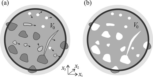
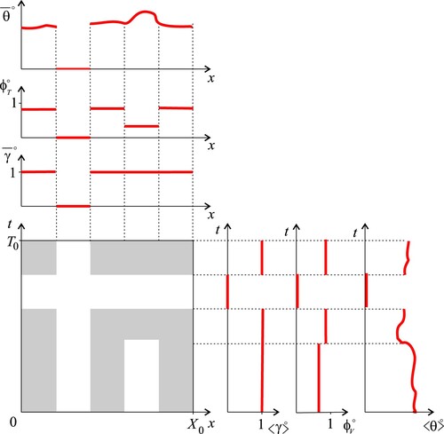
Figure A2. Results of the two possible first averaging steps for an idealized 1D case where the only spatial variations are in the x direction. The averaging windows in space and time are shown in the x, t plane: grey colour indicates the “wet” regions where water is present so the marker function $\gamma (x,t)$ is equal to one, and a generic fluid property $\theta (x,t)$ is defined, and white colour indicates “dry” regions where γ is zero. Results of each averaging step include intrinsic average of γ, occupancy ratio, and intrinsic (or superficial) average of θ, which are all functions of space if the first averaging step is time and vice-versa. The intrinsic average of γ can be used to track the other two functions

It is assumed that the averaging volume is sufficiently large to produce stable spatial averages but is also smaller than the scale of macroscopic spatial heterogeneities. It is also assumed that there is a clear separation between the time scales of turbulence and those of gradually varying unsteady flow. Time averaging is hence performed over a window $T_0$ which is sufficiently large to incorporate all scales of turbulence, but is also much smaller than the time scales of flow unsteadiness.

The first averaging step is performed over either time or volume. For a generic fluid quantity $\theta (x_i,t)$ which is defined wherever $\gamma (x_i,t)=1$, the respective definitions of the superficial time and volume averages performed in the first step are: (A1) $\begin{array}{rl}& {\overline{\theta }}^{s\circ }\left(x_i\right)=\frac{1}{T_0}{\int }_{T_0}\theta (x_i,t)\gamma (x_i,t)\mathrm{d}t,\\ & {〈\theta 〉}^{s\circ }\left(t\right)=\frac{1}{V_0}{\int }_{V_0}\theta (x_i,t)\gamma (x_i,t)\mathrm{d}V\end{array}$(A1) where the overbar indicates time average, square brackets indicate volume average, $T_0$ and $V_0$ are the averaging windows in time and space, respectively, superscript s indicates that an average is superficial, i.e. expressed using the entire averaging window, and a symbol “$\circ$” next to “s” stands for “one” and indicates the first averaging step.

For a general case with gaps in temporal and spatial averaging windows, parts of the averaging windows where the main fluid is present, i.e. where $\gamma (x_i,t)=1$ will be called “occupancy” time or volume, and defined as: $\begin{array}{rl}{T}_f^{\circ }\left(x_i\right)& ={\int }_{T_0}\gamma (x_i,t)\mathrm{d}t,\\ V_f^{\circ }\left(t\right)& ={\int }_{V_0}\gamma (x_i,t)\mathrm{d}V\end{array}$ It follows that occupancy time and volume have to be within the intervals $0\le T_f^{\circ }\left(x_i\right)\le T_0$ and $0\le V_f^{\circ }\left(t\right)\le V_0$, respectively. The occupancy time $T_f^{\circ }$ is zero for all spatial points located inside a stationary grain or another stationary solid object, whereas the occupancy volume $V_f^{\circ }$ is zero for all time instances when the entire averaging volume is dry (i.e. it does not contain the main fluid). The intrinsic averages, i.e. the averages expressed relative to the “occupied” parts of the averaging windows, are defined as: (A2) $\begin{array}{rl}{\overline{\theta }}^{\circ }\left(x_i\right)& =\{\begin{array}{ll}{\displaystyle \frac{1}{T_f^{\circ }}{\int }_{T_0}\theta (x_i,t)\gamma (x_i,t)\mathrm{d}t}& \mathrm{i}\mathrm{f}{T}_f^{\circ }\ne 0,\\ 0& \mathrm{i}\mathrm{f}{T}_f^{\circ }=0,\end{array}\\ {〈\theta 〉}^{\circ }\left(t\right)& =\{\begin{array}{ll}{\displaystyle \frac{1}{V_f^{\circ }}{\int }_{V_0}\theta (x_i,t)\gamma (x_i,t)\mathrm{d}V}& \mathrm{i}\mathrm{f}{V}_f^{\circ }\ne 0,\\ 0& \mathrm{i}\mathrm{f}{V}_f^{\circ }=0\end{array}\end{array}$(A2) The two kinds of averages are related via the ratios of “occupancy” time or volume and the corresponding averaging window: (A3) $\begin{array}{rl}& {\varphi }_{{}_T}^{\circ }\left(x_i\right)=\frac{T_f^{\circ }}{T_0}={\overline{\gamma (x_i,t)}}^{s\circ },\\ & {\varphi }_{{}_V}^{\circ }\left(t\right)=\frac{V_f^{\circ }}{V_0}={〈\gamma (x_i,t)〉}^{s\circ }\end{array}$(A3) In V. Nikora et al. (2013) and Papadopoulos et al. (2020) ${\varphi }_{{}_T}^{\circ }$ and ${\varphi }_{{}_V}^{\circ }$ are called time and spatial porosity, but in this paper they will be referred to as temporal and spatial occupancy ratios. From (A1(A1) $\begin{array}{rl}& {\overline{\theta }}^{s\circ }\left(x_i\right)=\frac{1}{T_0}{\int }_{T_0}\theta (x_i,t)\gamma (x_i,t)\mathrm{d}t,\\ & {〈\theta 〉}^{s\circ }\left(t\right)=\frac{1}{V_0}{\int }_{V_0}\theta (x_i,t)\gamma (x_i,t)\mathrm{d}V\end{array}$(A1) ), (A2) it follows that: (A4) $\begin{array}{rl}{\overline{\theta }}^{s\circ }& ={\varphi }_{{}_T}^{\circ }{\overline{\theta }}^{\circ },\\ {〈\theta 〉}^{s\circ }& ={\varphi }_{{}_V}^{\circ }{〈\theta 〉}^{\circ }\end{array}$(A4) The results of the first averaging step are functions of either space only, e.g. ${\overline{\theta }}^{s\circ }\left(x_i\right)$, ${\overline{\theta }}^{\circ }\left(x_i\right),$ or time only, e.g. ${〈\theta 〉}^{s\circ }\left(t\right)$, ${〈\theta 〉}^{\circ }\left(t\right)$ (Fig. A2). In either case it is necessary to track the regions where the first step occupancy time or volume are not zero, because the second step intrinsic averages have physically meaningful values only over these regions. Following time averaging, such regions are tracked over the averaging volume by ${\overline{\gamma }}^{\circ }\left(x_i\right)$, which has value 1 wherever $T_f\ne 0$ because the location has been visited by water at least once during $T_0$, and is zero otherwise (Fig. A2). Following volume averaging, “occupied regions” are tracked in time by ${〈\gamma 〉}^{\circ }\left(t\right)$, which is one at all time instances when the averaging volume contains at least a single particle of water. The two tracking functions are now used for the definition of the second step averages.

A general function $\psi \left(x_i\right)$ denotes a result of the first averaging step over time i.e. either ${\overline{\theta }}^{s\circ }$ or ${\overline{\theta }}^{\circ }$, or any other function with the same marker function ${\overline{\gamma }}^{\circ }\left(x_i\right)$, for instance ${\varphi }_{{}_T}^{\circ }$; Fig. A2. Similarly, $\phi \left(t\right)$ is a volume average (${〈\theta 〉}^{s\circ }$, or ${〈\theta 〉}^{\circ }$), or any other function marked by ${〈\gamma 〉}^{\circ }\left(t\right)$, such as ${\varphi }_V$. The second step superficial averages of $\psi \left(x_i\right)$ and $\phi \left(t\right)$ are therefore defined as: (A5) $\begin{array}{rl}& {〈\psi 〉}^s=\frac{1}{V_0}{\int }_{V_0}\psi \left(x_i\right){\overline{\gamma }}^{\circ }\left(x_i\right)\mathrm{d}V,\\ & {\overline{\phi }}^s=\frac{1}{T_0}{\int }_{T_0}\phi \left(t\right){〈\gamma 〉}^{\circ }\left(t\right)\mathrm{d}t\end{array}$(A5) The second step occupancy volume and time are: $\begin{array}{rl}& V_f={\int }_{V_0}{\overline{\gamma }}^{\circ }\left(x_i\right)\mathrm{d}V,\\ & T_f={\int }_{T_0}{〈\gamma 〉}^{\circ }\left(t\right)\mathrm{d}t\end{array}$ and the corresponding second step occupancy ratios are: (A6) $\begin{array}{rl}& {\varphi }_{{}_V}=\frac{V_f}{V_0}={〈{\overline{\gamma }}^{\circ }\left(x_i\right)〉}^s,\\ & {\varphi }_{{}_T}=\frac{T_f}{T_0}={\overline{{〈\gamma 〉}^{\circ }\left(t\right)}}^s\end{array}$(A6) Neither $V_f,T_f$ nor ${\varphi }_{{}_V}$, ${\varphi }_{{}_T}$ can be zero because that would happen only if the entire averaging volume has been dry throughout the entire time averaging window. For such case the fundamental equations describing the motion of the main fluid do not apply, so it is physically meaningless. The second step intrinsic averages are defined as: (A7) $\begin{array}{rl}& 〈\psi 〉=\frac{1}{V_f}{\int }_{V_0}\psi \left(x_i\right){\overline{\gamma }}^{\circ }\left(x_i\right)\mathrm{d}V,\\ & \overline{\phi }=\frac{1}{T_f}{\int }_{T_0}\phi \left(t\right){〈\gamma 〉}^{\circ }\left(t\right)\mathrm{d}t\end{array}$(A7) and they are related to second step superficial averages via: (A8) $\begin{array}{rl}{〈\psi 〉}^s& ={\varphi }_{{}_V}〈\psi 〉,\\ {\overline{\phi }}^s& ={\varphi }_{{}_T}\overline{\phi }\end{array}$(A8) Once all intrinsic averaging operators are defined it is possible to define the deviations from the intrinsic variables and the associated decomposition for fluid quantities.

• Time/space averaging An instantaneous value of $\theta (x_i,t)$ is decomposed into the first step intrinsic time average and the first step fluctuation: $\theta (x_i,t)={\overline{\theta \left(x_i\right)}}^{\circ }+{\theta }^{\mathrm{\prime }\circ }(x_i,t)$ A local value of $\psi \left(x_i\right)$, which is the result of the first averaging step (i.e. either ${\overline{\theta }}^{\circ }\left(x_i\right)$ or any other function defined over the same part of $V_0$, for instance ${\varphi }_{{}_V}^{\circ }$) is decomposed into the intrinsic volume average and the spatial disturbance: $\psi \left(x_i\right)=〈\psi 〉+\tilde{\psi }\left(x_i\right)$ The following rules of sum and product apply: (A9) $\begin{array}{rl}{\overline{{\theta }_1+{\theta }_2}}^{\circ }& ={\overline{{\theta }_1}}^{\circ }+{\overline{{\theta }_2}}^{\circ },\\ {\overline{{\theta }_1{\theta }_2}}^{\circ }& ={\overline{{\theta }_1}}^{\circ }{\overline{{\theta }_2}}^{\circ }+{\overline{{{\theta }_1}^{\mathrm{\prime }\circ }{{\theta }_2}^{\mathrm{\prime }\circ }}}^{\circ },\\ 〈{\psi }_1+{\psi }_2〉& =〈{\psi }_1〉+〈{\psi }_2〉,\\ 〈{\psi }_1{\psi }_2〉& =〈{\psi }_1〉〈{\psi }_2〉+〈\widetilde{{\psi }_1}\widetilde{{\psi }_2}〉\end{array}$(A9)

• Space/time averaging A local value of $\theta (x_i,t)$ is decomposed into the first step intrinsic volume average and the spatial disturbance: $\theta (x_i,t)={〈\theta 〉}^{\circ }\left(t\right)+{\tilde{\theta }}^{\circ }(x_i,t)$ An instantaneous value of $\phi \left(t\right)$, which is the result of the first averaging step (i.e. either ${〈\theta 〉}^{\circ }\left(t\right)$ or any other function defined over the same part of $T_0$, for instance ${\varphi }_{{}_T}^{\circ }$) is decomposed into the intrinsic time average and the fluctuation: $\phi \left(t\right)=\overline{\phi }+{\phi }^{\mathrm{\prime }}\left(t\right)$ The rules of sum and product analogous to Eq. (A9(A9) $\begin{array}{rl}{\overline{{\theta }_1+{\theta }_2}}^{\circ }& ={\overline{{\theta }_1}}^{\circ }+{\overline{{\theta }_2}}^{\circ },\\ {\overline{{\theta }_1{\theta }_2}}^{\circ }& ={\overline{{\theta }_1}}^{\circ }{\overline{{\theta }_2}}^{\circ }+{\overline{{{\theta }_1}^{\mathrm{\prime }\circ }{{\theta }_2}^{\mathrm{\prime }\circ }}}^{\circ },\\ 〈{\psi }_1+{\psi }_2〉& =〈{\psi }_1〉+〈{\psi }_2〉,\\ 〈{\psi }_1{\psi }_2〉& =〈{\psi }_1〉〈{\psi }_2〉+〈\widetilde{{\psi }_1}\widetilde{{\psi }_2}〉\end{array}$(A9) ) apply.

Appendix B. Relationships between superficial and intrinsic double averages

From the definitions of the averaging operators it follows that the two-step superficial averages commute, i.e. (B1) ${〈{\overline{\theta }}^{s\circ }〉}^s={\overline{{〈\theta 〉}^{s\circ }}}^s$(B1) For $\theta =\gamma$ it follows that: ${〈{\overline{\gamma (x_i,t)}}^{s\circ }〉}^s={\overline{{〈\gamma (x_i,t)〉}^{s\circ }}}^s={〈{\varphi }_{{}_T}^{\circ }〉}^s={\overline{{\varphi }_{{}_V}^{\circ }}}^s$ The relationships between double superficial averages and double intrinsic averages are developed by using the appropriate occupancy ratios (Eq. 1(1) $\begin{array}{r}\begin{array}{rlrl}{\overline{\theta }}^{s\circ }& ={\varphi }_{{}_T}^{\circ }{\overline{\theta }}^{\circ },& {〈\theta 〉}^{s\circ }& ={\varphi }_{{}_V}^{\circ }{〈\theta 〉}^{\circ },\\ {〈\psi 〉}^s& ={\varphi }_{{}_V}〈\psi 〉,& {\overline{\phi }}^s& ={\varphi }_{{}_T}\overline{\phi }\end{array}\end{array}$(1) ) to switch from superficial to intrinsic averages and vice versa, and the rules of sum and product for intrinsic averages. For time/space and space/time averaging, respectively, this yields: (B2) $\begin{array}{rl}{〈{\overline{\theta }}^{s\circ }〉}^s& ={\varphi }_{{}_V}〈{\varphi }_{{}_T}^{\circ }{\overline{\theta }}^{\circ }〉\\ & ={\varphi }_{{}_V}〈{\varphi }_{{}_T}^{\circ }〉〈{\overline{\theta }}^{\circ }〉+{\varphi }_{{}_V}〈\widetilde{{\varphi }_{{}_T}^{\circ }}\widetilde{{\overline{\theta }}^{\circ }}〉={〈{\varphi }_{{}_T}^{\circ }〉}^s〈{\overline{\theta }}^{\circ }〉+{〈\widetilde{{\varphi }_{{}_T}^{\circ }}\widetilde{{\overline{\theta }}^{\circ }}〉}^s,\\ {\overline{{〈\theta 〉}^{s\circ }}}^s& ={\varphi }_{{}_T}\overline{{\varphi }_{{}_V}^{\circ }{〈\theta 〉}^{\circ }}={\varphi }_{{}_T}\overline{{\varphi }_{{}_V}^{\circ }}\overline{{〈\theta 〉}^{\circ }}+{\varphi }_{{}_T}\overline{{\varphi }_{{}_V}^{{\circ }^{\prime }}{〈\theta 〉}^{{\circ }^{\prime }}}\\ & ={\overline{{\varphi }_{{}_V}^{\circ }}}^s\overline{{〈\theta 〉}^{\circ }}+{\overline{{\varphi }_{{}_V}^{{\circ }^{\prime }}{〈\theta 〉}^{{\circ }^{\prime }}}}^s\end{array}$(B2) These expressions indicate that the two-step intrinsic averages commute if the last terms in the Eq. (B2(B2) $\begin{array}{rl}{〈{\overline{\theta }}^{s\circ }〉}^s& ={\varphi }_{{}_V}〈{\varphi }_{{}_T}^{\circ }{\overline{\theta }}^{\circ }〉\\ & ={\varphi }_{{}_V}〈{\varphi }_{{}_T}^{\circ }〉〈{\overline{\theta }}^{\circ }〉+{\varphi }_{{}_V}〈\widetilde{{\varphi }_{{}_T}^{\circ }}\widetilde{{\overline{\theta }}^{\circ }}〉={〈{\varphi }_{{}_T}^{\circ }〉}^s〈{\overline{\theta }}^{\circ }〉+{〈\widetilde{{\varphi }_{{}_T}^{\circ }}\widetilde{{\overline{\theta }}^{\circ }}〉}^s,\\ {\overline{{〈\theta 〉}^{s\circ }}}^s& ={\varphi }_{{}_T}\overline{{\varphi }_{{}_V}^{\circ }{〈\theta 〉}^{\circ }}={\varphi }_{{}_T}\overline{{\varphi }_{{}_V}^{\circ }}\overline{{〈\theta 〉}^{\circ }}+{\varphi }_{{}_T}\overline{{\varphi }_{{}_V}^{{\circ }^{\prime }}{〈\theta 〉}^{{\circ }^{\prime }}}\\ & ={\overline{{\varphi }_{{}_V}^{\circ }}}^s\overline{{〈\theta 〉}^{\circ }}+{\overline{{\varphi }_{{}_V}^{{\circ }^{\prime }}{〈\theta 〉}^{{\circ }^{\prime }}}}^s\end{array}$(B2) ) are both zero, i.e. if neither ${\varphi }_{{}_T}^{\circ }$ and ${\overline{\theta }}^{\circ }$ nor ${\varphi }_{{}_V}^{\circ }$ and ${〈\theta 〉}^{\circ }$ are correlated. Providing real world examples when this condition is satisfied requires further investigations.

Another, simpler class of special cases when the intrinsic averages commute are those for which the interfaces between water and any other phase (i.e. grains, vegetation, air above free surface) are frozen, so that ${\varphi }_{{}_V}^{\circ }$ is constant and equal volumetric porosity, and ${\varphi }_{{}_T}^{\circ }$ is equal unity at all points occupied by water, hence making ${\overline{\theta }}^{s\circ }$ and ${\overline{\theta }}^{\circ }$ identical. For “frozen interfaces” cases both fluctuation and spatial disturbance operators commute with each other and with both kinds of averages, and the order of averaging steps for deriving double-averaged continuity and momentum equations does not affect the result (Pedras & de Lemos, 2000; Pokrajac et al., 2008).

The entire Appendices A and B so far have presented general definitions and rules applicable to a much broader range of cases than for the development of GSWEs. The remaining part of Appendices B and C are however dedicated to additional concepts and relationships needed for GSWEs.

The relationships (Eq. B2(B2) $\begin{array}{rl}{〈{\overline{\theta }}^{s\circ }〉}^s& ={\varphi }_{{}_V}〈{\varphi }_{{}_T}^{\circ }{\overline{\theta }}^{\circ }〉\\ & ={\varphi }_{{}_V}〈{\varphi }_{{}_T}^{\circ }〉〈{\overline{\theta }}^{\circ }〉+{\varphi }_{{}_V}〈\widetilde{{\varphi }_{{}_T}^{\circ }}\widetilde{{\overline{\theta }}^{\circ }}〉={〈{\varphi }_{{}_T}^{\circ }〉}^s〈{\overline{\theta }}^{\circ }〉+{〈\widetilde{{\varphi }_{{}_T}^{\circ }}\widetilde{{\overline{\theta }}^{\circ }}〉}^s,\\ {\overline{{〈\theta 〉}^{s\circ }}}^s& ={\varphi }_{{}_T}\overline{{\varphi }_{{}_V}^{\circ }{〈\theta 〉}^{\circ }}={\varphi }_{{}_T}\overline{{\varphi }_{{}_V}^{\circ }}\overline{{〈\theta 〉}^{\circ }}+{\varphi }_{{}_T}\overline{{\varphi }_{{}_V}^{{\circ }^{\prime }}{〈\theta 〉}^{{\circ }^{\prime }}}\\ & ={\overline{{\varphi }_{{}_V}^{\circ }}}^s\overline{{〈\theta 〉}^{\circ }}+{\overline{{\varphi }_{{}_V}^{{\circ }^{\prime }}{〈\theta 〉}^{{\circ }^{\prime }}}}^s\end{array}$(B2) ) can be expressed using the bulk water depth, H. Firstly, the definition of H given by Eq. (8(8) $H\left(t\right)={〈h(x_k,t〉}_A=\frac{1}{A_0}{\int }_{V_0}\gamma (x_k,z,t)\mathrm{d}V,k=1,2$(8) ) can be developed as: (B3) $H\left(t\right)=\frac{1}{A_0}{\int }_{V_0}\gamma (x_i,t)\mathrm{d}V=\frac{Z_0}{V_0}{\int }_{V_0}\gamma (x_i,t)\mathrm{d}V=Z_0{〈\gamma (x_i,t)〉}^{s\circ }$(B3) Comparison with (A3(A3) $\begin{array}{rl}& {\varphi }_{{}_T}^{\circ }\left(x_i\right)=\frac{T_f^{\circ }}{T_0}={\overline{\gamma (x_i,t)}}^{s\circ },\\ & {\varphi }_{{}_V}^{\circ }\left(t\right)=\frac{V_f^{\circ }}{V_0}={〈\gamma (x_i,t)〉}^{s\circ }\end{array}$(A3) ), shows that: (B4) $H\left(t\right)=Z_0{\varphi }_{{}_V}^{\circ }\left(t\right)$(B4) Secondly, averages of temporal and spatial occupancy rates (Eq. A3(A3) $\begin{array}{rl}& {\varphi }_{{}_T}^{\circ }\left(x_i\right)=\frac{T_f^{\circ }}{T_0}={\overline{\gamma (x_i,t)}}^{s\circ },\\ & {\varphi }_{{}_V}^{\circ }\left(t\right)=\frac{V_f^{\circ }}{V_0}={〈\gamma (x_i,t)〉}^{s\circ }\end{array}$(A3) ) can be related to H via: (B5) $\begin{array}{rl}{〈{\overline{\gamma (x_i,t)}}^{s\circ }〉}^s& ={\overline{{〈\gamma (x_i,t)〉}^{s\circ }}}^s={〈{\varphi }_{{}_T}^{\circ }〉}^s={\overline{{\varphi }_{{}_V}^{\circ }}}^s\\ & =\frac{1}{T_0}\frac{1}{V_0}{\int }_{T_0}{\int }_{V_0}\gamma (x_i,t)\mathrm{d}V\mathrm{d}t\\ & =\frac{1}{T_0}\frac{1}{Z_0}\frac{1}{A_0}{\int }_{T_0}{\int }_{V_0}\gamma (x_i,t)\mathrm{d}V\mathrm{d}t\\ & =\frac{1}{T_0}\frac{1}{Z_0}{\int }_{T_0}H\left(t\right)\mathrm{d}t=\frac{1}{Z_0}{\overline{H}}^s\end{array}$(B5) Recalling that time-averaged bulk water depth can be related to bulk flow layer height via ${\overline{H}}^s={\varphi }_{{}_H}{H}_0$ the above equation can be summarized as: (B6) $Z_0{〈{\varphi }_{{}_T}^{\circ }〉}^s=Z_0{\overline{{\varphi }_{{}_V}^{\circ }}}^s={\overline{H}}^s={\varphi }_{{}_H}{H}_0$(B6) so that the relationships (Eq. B2(B2) $\begin{array}{rl}{〈{\overline{\theta }}^{s\circ }〉}^s& ={\varphi }_{{}_V}〈{\varphi }_{{}_T}^{\circ }{\overline{\theta }}^{\circ }〉\\ & ={\varphi }_{{}_V}〈{\varphi }_{{}_T}^{\circ }〉〈{\overline{\theta }}^{\circ }〉+{\varphi }_{{}_V}〈\widetilde{{\varphi }_{{}_T}^{\circ }}\widetilde{{\overline{\theta }}^{\circ }}〉={〈{\varphi }_{{}_T}^{\circ }〉}^s〈{\overline{\theta }}^{\circ }〉+{〈\widetilde{{\varphi }_{{}_T}^{\circ }}\widetilde{{\overline{\theta }}^{\circ }}〉}^s,\\ {\overline{{〈\theta 〉}^{s\circ }}}^s& ={\varphi }_{{}_T}\overline{{\varphi }_{{}_V}^{\circ }{〈\theta 〉}^{\circ }}={\varphi }_{{}_T}\overline{{\varphi }_{{}_V}^{\circ }}\overline{{〈\theta 〉}^{\circ }}+{\varphi }_{{}_T}\overline{{\varphi }_{{}_V}^{{\circ }^{\prime }}{〈\theta 〉}^{{\circ }^{\prime }}}\\ & ={\overline{{\varphi }_{{}_V}^{\circ }}}^s\overline{{〈\theta 〉}^{\circ }}+{\overline{{\varphi }_{{}_V}^{{\circ }^{\prime }}{〈\theta 〉}^{{\circ }^{\prime }}}}^s\end{array}$(B2) ) can be written as: (B7) $\begin{array}{rl}{Z}_0{〈{\overline{\theta }}^{s\circ }〉}^s& =Z_0{\overline{{〈\theta 〉}^{s\circ }}}^s={\overline{H}}^s〈{\overline{\theta }}^{\circ }〉+Z_0{〈\widetilde{{\varphi }_{{}_T}^{\circ }}\widetilde{{\overline{\theta }}^{\circ }}〉}^s\\ & ={\overline{H}}^s\overline{{〈\theta 〉}^{\circ }}+Z_0{\overline{{\varphi }_{{}_V}^{{\circ }^{\prime }}{〈\theta 〉}^{{\circ }^{\prime }}}}^s\end{array}$(B7) It can be shown that for space-time averaging the fluctuations of the instantaneous bulk water depth are related to the fluctuations of the instantaneous spatial occupancy ratio via: (B8) $H^{\mathrm{\prime }}=Z_0{{\varphi }_{{}_V}^{\circ }}^{\mathrm{\prime }}$(B8) so that the last term in Eq. (B7(B7) $\begin{array}{rl}{Z}_0{〈{\overline{\theta }}^{s\circ }〉}^s& =Z_0{\overline{{〈\theta 〉}^{s\circ }}}^s={\overline{H}}^s〈{\overline{\theta }}^{\circ }〉+Z_0{〈\widetilde{{\varphi }_{{}_T}^{\circ }}\widetilde{{\overline{\theta }}^{\circ }}〉}^s\\ & ={\overline{H}}^s\overline{{〈\theta 〉}^{\circ }}+Z_0{\overline{{\varphi }_{{}_V}^{{\circ }^{\prime }}{〈\theta 〉}^{{\circ }^{\prime }}}}^s\end{array}$(B7) ) can be written as ${\overline{H^{\mathrm{\prime }}{〈\theta 〉}^{{\circ }^{\prime }}}}^s.$

For θ representing a microscopically constant property such as the main fluid density, ρ, both terms with deviations in Eq. (B7(B7) $\begin{array}{rl}{Z}_0{〈{\overline{\theta }}^{s\circ }〉}^s& =Z_0{\overline{{〈\theta 〉}^{s\circ }}}^s={\overline{H}}^s〈{\overline{\theta }}^{\circ }〉+Z_0{〈\widetilde{{\varphi }_{{}_T}^{\circ }}\widetilde{{\overline{\theta }}^{\circ }}〉}^s\\ & ={\overline{H}}^s\overline{{〈\theta 〉}^{\circ }}+Z_0{\overline{{\varphi }_{{}_V}^{{\circ }^{\prime }}{〈\theta 〉}^{{\circ }^{\prime }}}}^s\end{array}$(B7) ) are zero so that it reduces to: (B9) $Z_0{〈{\overline{\rho }}^{s\circ }〉}^s={\overline{H}}^s〈{\overline{\rho }}^{\circ }〉={\overline{H}}^s\rho$(B9) Finally, it is necessary to develop the the relationship between double superficial average and double intrinsic average of a product. It is needed solely for the advective term in the momentum equation, so the derivation is shown for the product $u_i{u}_j$ rather than for generic fluid quantities. For time/space averaging it starts with: ${〈{\overline{u_i{u}_j}}^{s\circ }〉}^s={\varphi }_{{}_V}〈{\varphi }_{{}_T}^{\circ }{\overline{u_i{u}_j}}^{\circ }〉={\varphi }_{{}_V}〈{\varphi }_{{}_T}^{\circ }{\overline{u_i}}^{\circ }{\overline{u_j}}^{\circ }〉+{\varphi }_{{}_V}〈{\varphi }_{{}_T}^{\circ }{\overline{{u_i}^{\mathrm{\prime }\circ }{u_j}^{\mathrm{\prime }\circ }}}^{\circ }〉$ The two last terms are developed separately as: $\begin{array}{rl}{\varphi }_{{}_V}〈{\varphi }_{{}_T}^{\circ }{\overline{u_i}}^{\circ }{\overline{u_j}}^{\circ }〉& ={\varphi }_{{}_V}〈{\varphi }_{{}_T}^{\circ }〉〈{\overline{u_i}}^{\circ }〉〈{\overline{u_j}}^{\circ }〉+{\varphi }_{{}_V}〈{\varphi }_{{}_T}^{\circ }〉〈\stackrel{~}{{\overline{u_i}}^{\circ }}\stackrel{~}{{\overline{u_j}}^{\circ }}〉\\ & +{\varphi }_{{}_V}〈{\overline{u_j}}^{\circ }〉〈\widetilde{{\varphi }_{{}_T}^{\circ }}\stackrel{~}{{\overline{u_i}}^{\circ }}〉+{\varphi }_{{}_V}〈{\overline{u_i}}^{\circ }〉〈\widetilde{{\varphi }_{{}_T}^{\circ }}\stackrel{~}{{\overline{u_j}}^{\circ }}〉\\ & ={〈{\varphi }_{{}_T}^{\circ }〉}^s〈{\overline{u_i}}^{\circ }〉〈{\overline{u_j}}^{\circ }〉+{〈{\varphi }_{{}_T}^{\circ }〉}^s〈\stackrel{~}{{\overline{u_i}}^{\circ }}\stackrel{~}{{\overline{u_j}}^{\circ }}〉\\ & +{〈{\overline{u_j}}^{\circ }〉}^s〈\widetilde{{\varphi }_{{}_T}^{\circ }}\stackrel{~}{{\overline{u_i}}^{\circ }}〉+{〈{\overline{u_i}}^{\circ }〉}^s〈\widetilde{{\varphi }_{{}_T}^{\circ }}\stackrel{~}{{\overline{u_j}}^{\circ }}〉,\\ {\varphi }_{{}_V}〈{\varphi }_{{}_T}^{\circ }{\overline{{u_i}^{\mathrm{\prime }\circ }{u_j}^{\mathrm{\prime }\circ }}}^{\circ }〉& ={\varphi }_{{}_V}〈{\varphi }_{{}_T}^{\circ }〉〈{\overline{{u_i}^{\mathrm{\prime }\circ }{u_j}^{\mathrm{\prime }\circ }}}^{\circ }〉+{\varphi }_{{}_V}〈\widetilde{{\varphi }_{{}_T}^{\circ }}\stackrel{~}{{\overline{{u_i}^{\mathrm{\prime }\circ }{u_j}^{\mathrm{\prime }\circ }}}^{\circ }}〉\\ & ={〈{\varphi }_{{}_T}^{\circ }〉}^s〈{\overline{{u_i}^{\mathrm{\prime }\circ }{u_j}^{\mathrm{\prime }\circ }}}^{\circ }〉+{〈\widetilde{{\varphi }_{{}_T}^{\circ }}\stackrel{~}{{\overline{{u_i}^{\mathrm{\prime }\circ }{u_j}^{\mathrm{\prime }\circ }}}^{\circ }}〉}^s\end{array}$ Remembering that $Z_0{〈{\varphi }_{{}_T}^{\circ }〉}^s={\overline{H}}^s$ (Eq. B6(B6) $Z_0{〈{\varphi }_{{}_T}^{\circ }〉}^s=Z_0{\overline{{\varphi }_{{}_V}^{\circ }}}^s={\overline{H}}^s={\varphi }_{{}_H}{H}_0$(B6) ) the previous three relationships can be combined into: (B10) $\begin{array}{rl}{Z}_0{〈{\overline{u_i{u}_j}}^{s\circ }〉}^s& ={\overline{H}}^s〈{\overline{u_i}}^{\circ }〉〈{\overline{u_j}}^{\circ }〉+{\overline{H}}^s〈\stackrel{~}{{\overline{u_i}}^{\circ }}\stackrel{~}{{\overline{u_j}}^{\circ }}〉+{\overline{H}}^s〈{\overline{{u_i}^{\mathrm{\prime }\circ }{u_j}^{\mathrm{\prime }\circ }}}^{\circ }〉\\ & +Z_0{〈{\overline{u_j}}^{\circ }〉}^s〈\widetilde{{\varphi }_{{}_T}^{\circ }}\stackrel{~}{{\overline{u_i}}^{\circ }}〉+Z_0{〈{\overline{u_i}}^{\circ }〉}^s〈\widetilde{{\varphi }_{{}_T}^{\circ }}\stackrel{~}{{\overline{u_j}}^{\circ }}〉\\ & +Z_0{〈\widetilde{{\varphi }_{{}_T}^{\circ }}\stackrel{~}{{\overline{{u_i}^{\mathrm{\prime }\circ }{u_j}^{\mathrm{\prime }\circ }}}^{\circ }}〉}^s\end{array}$(B10) The derivation for space/time averaging is analogous: $\begin{array}{rl}{\overline{〈u_i{u}_j{〉}^{s\circ }}}^s& ={\varphi }_{{}_T}\overline{{\varphi }_{{}_V}^{\circ }〈u_i{u}_j{〉}^{\circ }}={\varphi }_{{}_T}\overline{{\varphi }_{{}_V}^{\circ }〈u_i{〉}^{\circ }〈u_j{〉}^{\circ }}\\ & +{\varphi }_{{}_T}{\overline{{\varphi }_{{}_V}^{\circ }〈{\widetilde{u_i}}^{\circ }{\widetilde{u_j}}^{\circ }〉}}^{\circ },\\ {\varphi }_{{}_T}\overline{{\varphi }_{{}_V}^{\circ }{〈u_i〉}^{\circ }{〈u_j〉}^{\circ }}& ={\varphi }_{{}_T}\overline{{\varphi }_{{}_V}^{\circ }}\overline{〈u_i{〉}^{\circ }}\overline{〈u_j{〉}^{\circ }}+{\varphi }_{{}_T}\overline{{\varphi }_{{}_V}^{\circ }}\overline{〈u_i{〉}^{{\circ }^{\prime }}}{〈u_j〉}^{{\circ }^{\prime }}\\ & +{\varphi }_{{}_T}\overline{{〈u_j〉}^{\circ }}\overline{{\varphi }_{{}_V}^{{\circ }^{\prime }}{〈u_i〉}^{{\circ }^{\prime }}}+{\varphi }_{{}_T}\overline{{〈u_i〉}^{\circ }}\overline{{\varphi }_{{}_V}^{{\circ }^{\prime }}{〈u_j〉}^{{\circ }^{\prime }}}\\ & ={\overline{{\varphi }_{{}_V}^{\circ }}}^s\overline{{〈u_i〉}^{\circ }}\overline{{〈u_j〉}^{\circ }}+{\overline{{\varphi }_{{}_V}^{\circ }}}^s\overline{{〈u_i〉}^{{\circ }^{\prime }}{〈u_j〉}^{{\circ }^{\prime }}}\\ & +{\overline{{〈u_j〉}^{\circ }}}^s\overline{{\varphi }_{{}_V}^{{\circ }^{\prime }}{〈u_i〉}^{{\circ }^{\prime }}}+{\overline{{〈u_i〉}^{\circ }}}^s\overline{{\varphi }_{{}_V}^{{\circ }^{\prime }}{〈u_j〉}^{{\circ }^{\prime }}},\\ {\varphi }_{{}_T}\overline{{\varphi }_{{}_V}^{\circ }{〈{\widetilde{u_i}}^{\circ }{\widetilde{u_j}}^{\circ }〉}^{\circ }}& ={\varphi }_{{}_T}\overline{{\varphi }_{{}_V}^{\circ }}\overline{{〈{\widetilde{u_i}}^{\circ }{\widetilde{u_j}}^{\circ }〉}^{\circ }}+{\varphi }_{{}_T}\overline{{\varphi }_{{}_V}^{{\circ }^{\prime }}{〈{\widetilde{u_i}}^{\circ }{\widetilde{u_j}}^{\circ }〉}^{{\circ }^{\prime }}}\\ & ={\overline{{\varphi }_{{}_V}^{\circ }}}^s\overline{{〈{\widetilde{u_i}}^{\circ }{\widetilde{u_j}}^{\circ }〉}^{\circ }}+{\overline{{\varphi }_{{}_V}^{{\circ }^{\prime }}{〈{\widetilde{u_i}}^{\circ }{\widetilde{u_j}}^{\circ }〉}^{{\circ }^{\prime }}}}^s\end{array}$ In terms of bulk water depth, using Eq. (B6(B7) $\begin{array}{rl}{Z}_0{〈{\overline{\theta }}^{s\circ }〉}^s& =Z_0{\overline{{〈\theta 〉}^{s\circ }}}^s={\overline{H}}^s〈{\overline{\theta }}^{\circ }〉+Z_0{〈\widetilde{{\varphi }_{{}_T}^{\circ }}\widetilde{{\overline{\theta }}^{\circ }}〉}^s\\ & ={\overline{H}}^s\overline{{〈\theta 〉}^{\circ }}+Z_0{\overline{{\varphi }_{{}_V}^{{\circ }^{\prime }}{〈\theta 〉}^{{\circ }^{\prime }}}}^s\end{array}$(B7) ): (B11) $\begin{array}{rl}{Z}_0{\overline{{〈u_i{u}_j〉}^{s\circ }}}^s& ={\overline{H}}^s\overline{{〈u_i〉}^{\circ }}\overline{{〈u_j〉}^{\circ }}+{\overline{H}}^s\overline{{〈u_i〉}^{{\circ }^{\prime }}{〈u_j〉}^{{\circ }^{\prime }}}+{\overline{H}}^s\overline{{〈{\widetilde{u_i}}^{\circ }{\widetilde{u_j}}^{\circ }〉}^{\circ }}\\ & +Z_0{\overline{{〈u_j〉}^{\circ }}}^s\overline{{\varphi }_{{}_V}^{{\circ }^{\prime }}{〈u_i〉}^{{\circ }^{\prime }}}+Z_0{\overline{{〈u_i〉}^{\circ }}}^s\overline{{\varphi }_{{}_V}^{{\circ }^{\prime }}{〈u_j〉}^{{\circ }^{\prime }}}\\ & +Z_0{\overline{{\varphi }_{{}_V}^{{\circ }^{\prime }}{〈{\widetilde{u_i}}^{\circ }{\widetilde{u_j}}^{\circ }〉}^{{\circ }^{\prime }}}}^s\end{array}$(B11)

Appendix C. Hydrostatic pressure

In order to determine pressure at the bottom surface and double-averaged pressure for the entire averaging volume $V_0$ used for deriving GSWEs (Fig. 1) it is useful to develop an expression for pressure at the bottom of the water column, and at an arbitrary level z, both for an arbitrary x, y location. This can be achieved by using the double-averaged momentum equation for the z direction, but this time with the spatial averaging done over a cylinder with a base $\mathrm{d}{A}_0=\mathrm{d}x\mathrm{d}y$ centred at x, y, which contains at least a single point that gets wet for at least a single time instant. The equation is analogous to the double-averaged momentum equation (20(20) $\begin{array}{rl}& Z_0\frac{\mathrm{\partial }{〈{\overline{u_j}}^{s\circ }〉}^s}{\mathrm{\partial }t}+Z_0\frac{\mathrm{\partial }{〈{\overline{u_k{u}_j}}^{s\circ }〉}^s}{\mathrm{\partial }{x}_k}\\ & =Z_0{〈{\overline{g_j}}^{s\circ }〉}^s-\frac{Z_0}{\rho }\frac{\mathrm{\partial }{〈{\overline{p}}^{s\circ }〉}^s}{\mathrm{\partial }{x}_j}+\frac{Z_0}{\rho }\frac{\mathrm{\partial }{〈{\overline{{\tau }_{kj}}}^{s\circ }〉}^s}{\mathrm{\partial }{x}_k}\\ & +\frac{{\overline{f_j}}^s}{\rho }+q_j^{bot}+q_j^{top},j,k=1,2\end{array}$(20) ) for j = 3 instead of j = 1, 2, except that it does not contain the term with the z-gradient of pressure (for the same reason all other z-gradients are zero). Furthermore, water depth and flow layer height are denoted by h and $h_0$, respectively, (rather than H and $H_0$), because averaging has been done over an infinitesimally small plan area, and momentum exchange terms $q_z^{top}$ and $q_z^{bot}$ are assumed zero. The macroscopic z-momentum equation is: (C1) $\begin{array}{rl}& Z_0\frac{\mathrm{\partial }{〈{\overline{w}}^{s\circ }〉}^s}{\mathrm{\partial }t}+Z_0\frac{\mathrm{\partial }{〈{\overline{u_{k}w}}^{s\circ }〉}^s}{\mathrm{\partial }{x}_k}\\ & =Z_0{〈{\overline{g_z}}^{s\circ }〉}^s+\frac{Z_0}{\rho }\frac{\mathrm{\partial }{〈{\overline{{\tau }_{kz}}}^{s\circ }〉}^s}{\mathrm{\partial }{x}_k}+\frac{{\overline{f_z}}^s}{\rho },k=1,2\end{array}$(C1) where $\begin{array}{rl}{Z}_0{〈{\overline{g_z}}^{s\circ }〉}^s& =-g{\overline{h}}^s\cos {\alpha }_x\cos {\alpha }_y,\\ f_z& =f_z^{int}+f_z^{bot}+f_z^{top},\\ f_z^{int/bot/top}& =\frac{1}{\mathrm{d}{A}_0}p{|}_{{}_{int/bot/top}}{n}_z\mathrm{d}{S}_{int/bot/top}\\ & -\frac{1}{\mathrm{d}{A}_0}{\tau }_{iz}{|}_{{}_{int/bot/top}}{n}_i\mathrm{d}{S}_{int/bot/top},i=1,2,3\end{array}$ Hydrostatic pressure distribution implies that all terms in Eq. (C1(C1) $\begin{array}{rl}& Z_0\frac{\mathrm{\partial }{〈{\overline{w}}^{s\circ }〉}^s}{\mathrm{\partial }t}+Z_0\frac{\mathrm{\partial }{〈{\overline{u_{k}w}}^{s\circ }〉}^s}{\mathrm{\partial }{x}_k}\\ & =Z_0{〈{\overline{g_z}}^{s\circ }〉}^s+\frac{Z_0}{\rho }\frac{\mathrm{\partial }{〈{\overline{{\tau }_{kz}}}^{s\circ }〉}^s}{\mathrm{\partial }{x}_k}+\frac{{\overline{f_z}}^s}{\rho },k=1,2\end{array}$(C1) ) other than gravity and $f_z$ are negligible. Furthermore, the force acting at the top of the flow layer, $f_z^{top}$, is assumed to be zero. The resulting z-momentum equation is: (C2) $\rho g{\overline{h}}^s\cos {\alpha }_x\cos {\alpha }_y={\overline{f_z^{int}}}^s+{\overline{f_z^{bot}}}^s$(C2) The viscous stress components of both $f_z^{int}$ and $f_z^{bot}$ are neglected so that: (C3) $\begin{array}{rl}{f}_z^{int}& =\frac{1}{\mathrm{d}{A}_0}p{|}_{{}_{int}}{n}_z\mathrm{d}{S}_{int}=p_{int},\\ f_z^{bot}& =\frac{1}{\mathrm{d}{A}_0}p{|}_{{}_{bot}}{n}_z\mathrm{d}{S}_{bot}=p_{bot}\end{array}$(C3) where $p_{int}$ is the magnitude of the buoyancy force, per unit plan area, exerted by all internal interfaces within the water column, and $p_{bot}$ is the hydrostatic pressure at the bottom boundary.

Combining Eqs (C2(C2) $\rho g{\overline{h}}^s\cos {\alpha }_x\cos {\alpha }_y={\overline{f_z^{int}}}^s+{\overline{f_z^{bot}}}^s$(C2) ) and (C3(C3) $\begin{array}{rl}{f}_z^{int}& =\frac{1}{\mathrm{d}{A}_0}p{|}_{{}_{int}}{n}_z\mathrm{d}{S}_{int}=p_{int},\\ f_z^{bot}& =\frac{1}{\mathrm{d}{A}_0}p{|}_{{}_{bot}}{n}_z\mathrm{d}{S}_{bot}=p_{bot}\end{array}$(C3) ) yields: (C4) ${\overline{p_{int}}}^s+{\overline{p_{bot}}}^s=\rho g{\overline{h}}^s\cos {\alpha }_x\cos {\alpha }_y$(C4) Buoyancy force is exerted by all dry parts of the water column and its direction is downwards. The total height of the dry parts at any time instant is $z_{{}_{TOP}}-z_{bot}-{\overline{h}}^s$, so ${\overline{p_{int}}}^s$ can be also expressed as: (C5) ${\overline{p_{int}}}^s=-\rho g(z_{{}_{TOP}}-z_{bot}-{\overline{h}}^s)\cos {\alpha }_x\cos {\alpha }_y$(C5) Combining Eqs (C5(C5) ${\overline{p_{int}}}^s=-\rho g(z_{{}_{TOP}}-z_{bot}-{\overline{h}}^s)\cos {\alpha }_x\cos {\alpha }_y$(C5) ) with (C4(C4) ${\overline{p_{int}}}^s+{\overline{p_{bot}}}^s=\rho g{\overline{h}}^s\cos {\alpha }_x\cos {\alpha }_y$(C4) ) produces, for the bottom pressure: (C6) ${\overline{p_{bot}}}^s=\rho g(z_{{}_{TOP}}-z_{bot})\cos {\alpha }_x\cos {\alpha }_y$(C6) The bottom pressure (Eq. C6(C6) ${\overline{p_{bot}}}^s=\rho g(z_{{}_{TOP}}-z_{bot})\cos {\alpha }_x\cos {\alpha }_y$(C6) ) acts across the entire bottom surface, except for the gaps in this surface caused by the internal objects rooted into the bed. These gaps are not in contact with water, hence the bottom pressure across them is not defined. The part of the bottom surface where pressure is defined, projected onto the bottom boundary, is tracked by a marker function ${\gamma }_{{}_{BOT}}$, and projected onto the $(x,y)$ plane, by ${\gamma }_{{}_A}$. The area of the part of $A_0$ where ${\gamma }_{{}_A}$ is equal unity is $C_A^{bot}{A}_0$. Equation (C6(C6) ${\overline{p_{bot}}}^s=\rho g(z_{{}_{TOP}}-z_{bot})\cos {\alpha }_x\cos {\alpha }_y$(C6) ) is now plugged into the first term on the r.h.s. of Eq. (28(28) $\begin{array}{rl}{f}_j^{int/bot}& =\frac{1}{A_0}{\int }_{S_{int/bot}}{p}_{int/bot}{n}_j\mathrm{d}S\\ & +\frac{1}{A_0}{\int }_{S_{int/bot}}(p-p_{int/bot})n_j\mathrm{d}S\\ & -\frac{1}{A_0}{\int }_{S_{int/bot}}{\tau }_{ij}{n}_i\mathrm{d}S,i=1,2,3,j=1,2\end{array}$(28) ) in order to develop the expression for the j component of the hydrostatic force on the entire bottom surface: (C7) $\frac{1}{A_0}{\int }_{S_{bot}}{\overline{p_{bot}}}^s{n}_j\mathrm{d}S=\rho g\frac{1}{A_0}{\int }_{S_{bot}}(z_{{}_{TOP}}-z_{bot})n_j\mathrm{d}S\cos {\alpha }_x\cos {\alpha }_y$(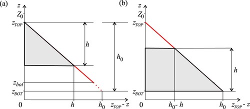C7)

Figure C1. Hydrostatic pressure distribution over flow profiles containing a wet part of height h (grey), and a part that remains dry throughout the entire time averaging window. (Red line shows what the pressure profile would be if the entire space between $z_{{}_{TOP}}$ and $z_{bot}$ was wet.) Pressure force is proportional to the areas shaded grey. It is smallest when the wet part is at the top of the profile (a), and largest when it is at the bottom (b)

The integral over $S_{bot}$ in the above equation is developed as: (C8) $\begin{array}{rl}{\int }_{S_{bot}}(z_{{}_{TOP}}-z_{bot})n_j\mathrm{d}S& ={\int }_{S_{bot}}(z_{{}_{TOP}}-z_{{}_{BOT}}+z_{{}_{BOT}}-z_{bot})n_j\mathrm{d}S\\ & ={\int }_{S_{bot}}(z_{{}_{TOP}}-z_{{}_{BOT}})n_j\mathrm{d}S\\ & ={\int }_{S_{{}_{BOT}}}{\gamma }_{{}_{BOT}}(z_{{}_{TOP}}-z_{{}_{BOT}})\mathrm{d}S\\ & ={\int }_{A_0}{\gamma }_{{}_A}(z_{{}_{TOP}}-z_{{}_{BOT}})\sin {\text{β}}_j\mathrm{d}A\\ & ={\int }_{A_0}{\gamma }_A{h}_0\mathrm{d}A\sin {\text{β}}_j=A_0{C}_A^{bot}{H}_0\sin {\text{β}}_j\end{array}$(C8) Plugging the final expression for the integral over $S_{bot}$ into Eq. (C7(C7) $\frac{1}{A_0}{\int }_{S_{bot}}{\overline{p_{bot}}}^s{n}_j\mathrm{d}S=\rho g\frac{1}{A_0}{\int }_{S_{bot}}(z_{{}_{TOP}}-z_{bot})n_j\mathrm{d}S\cos {\alpha }_x\cos {\alpha }_y$(C7) ) yields: (C9) $\frac{1}{A_0}{\int }_{S_{bot}}{\overline{p_{bot}}}^s{n}_j\mathrm{d}S=\rho g{C}_A^{bot}{H}_0\sin {\text{β}}_j\cos {\alpha }_x\cos {\alpha }_y$(C9) The expression for the hydrostatic pressure at an arbitrary level z is derived in an analogues manner as Eq. (C6(C6) ${\overline{p_{bot}}}^s=\rho g(z_{{}_{TOP}}-z_{bot})\cos {\alpha }_x\cos {\alpha }_y$(C6) ), this time with z instead of $z_{bot}$. The result is: (C10) ${\overline{p_z}}^s\left(z\right)=\rho g{h}_{0z}\cos {\alpha }_x\cos {\alpha }_y=\rho g\cos {\alpha }_x\cos {\alpha }_y(z_{{}_{TOP}}-z)$(C10) where $h_{0z}=z_{{}_{TOP}}-z$ is the flow layer height above z. It should be noted that ${\overline{p_z}}^s$ is defined only at the z points that get wet for at lest single time instant during time averaging window, i.e. for the z points for which the intrinsic time average of the marker function γ is equal to one.

The time-averaged hydrostatic pressure at z expressed by Eq. (C10(C10) ${\overline{p_z}}^s\left(z\right)=\rho g{h}_{0z}\cos {\alpha }_x\cos {\alpha }_y=\rho g\cos {\alpha }_x\cos {\alpha }_y(z_{{}_{TOP}}-z)$(C10) ) is now averaged over the entire averaging volume in order to find the double-averaged hydrostatic pressure. The result is: (C11) $\begin{array}{rl}{〈{\overline{p}}^{s\circ }〉}^s& =\frac{1}{Z_0{A}_0}{\int }_{A_0}{\int }_0^{Z_0}{\overline{\gamma }}^{\circ }\left(z\right){\overline{p}}^{s\circ }\left(z\right)\mathrm{d}z\mathrm{d}{A}_0\\ & =\frac{\rho g}{Z_0{A}_0}\cos {\alpha }_x\cos {\alpha }_y{\int }_{A_0}{\int }_{z_{{}_{BOT}}}^{z_{{}_{TOP}}}{\overline{\gamma }}^{\circ }\left(z\right)(z_{{}_{TOP}}-z)\mathrm{d}z\mathrm{d}{A}_0\end{array}$(C11) Note that the boundaries of integration over z were changed from $(0,Z_0)$ to $(z_{{}_{BOT}},z_{{}_{TOP}})$ because $\gamma \left(z\right)=0$ below $z_{{}_{BOT}}$ and above $z_{{}_{TOP}}$.

If a flow layer contains just clear water and the bottom surface is flat ($z_{bot}=z_{{}_{BOT}}$), the integral over z in Eq. (C11(C11) $\begin{array}{rl}{〈{\overline{p}}^{s\circ }〉}^s& =\frac{1}{Z_0{A}_0}{\int }_{A_0}{\int }_0^{Z_0}{\overline{\gamma }}^{\circ }\left(z\right){\overline{p}}^{s\circ }\left(z\right)\mathrm{d}z\mathrm{d}{A}_0\\ & =\frac{\rho g}{Z_0{A}_0}\cos {\alpha }_x\cos {\alpha }_y{\int }_{A_0}{\int }_{z_{{}_{BOT}}}^{z_{{}_{TOP}}}{\overline{\gamma }}^{\circ }\left(z\right)(z_{{}_{TOP}}-z)\mathrm{d}z\mathrm{d}{A}_0\end{array}$(C11) ) yields $h_0^2/2=h^2/2$ and integrating this term over $A_0$ produces $H_0^2/2$. In a general case when some parts of z profiles are dry, finding the analytical expression for the integral over z is straightforward only if the distribution of the wet parts of the water column is known. For a general case with an unknown distribution it is not possible to solve the integral analytically. However, with the reference to Fig. C1 it is clear that the integral cannot be smaller than ${\overline{h}}^s{\overline{h}}^s/2$ (when all wet parts are at the top of the column, Fig. C1a), nor larger than $(2h_0/{\overline{h}}^s-1){\overline{h}}^s{\overline{h}}^s/2$ (when they are at the bottom, Fig. C1b). The integral over z in the last term of (C11(C11) $\begin{array}{rl}{〈{\overline{p}}^{s\circ }〉}^s& =\frac{1}{Z_0{A}_0}{\int }_{A_0}{\int }_0^{Z_0}{\overline{\gamma }}^{\circ }\left(z\right){\overline{p}}^{s\circ }\left(z\right)\mathrm{d}z\mathrm{d}{A}_0\\ & =\frac{\rho g}{Z_0{A}_0}\cos {\alpha }_x\cos {\alpha }_y{\int }_{A_0}{\int }_{z_{{}_{BOT}}}^{z_{{}_{TOP}}}{\overline{\gamma }}^{\circ }\left(z\right)(z_{{}_{TOP}}-z)\mathrm{d}z\mathrm{d}{A}_0\end{array}$(C11) ) can therefore be expressed as: (C12) ${\int }_0^{Z_0}{\overline{\gamma }}^{\circ }\left(z\right)(z_{{}_{TOP}}-z)\mathrm{d}z=C_p\frac{{\overline{h}}^s{\overline{h}}^s}{2}$(C12) where $1\le C_p(x,y)\le 2h_0/{\overline{h}}^s-1$ accounts for the distribution of the wet parts of the profile, including its variability with time, and the expression applies only for the profiles which contain at least a single wet point for at least a single time instant.

Plugging Eq. (C12(C12) ${\int }_0^{Z_0}{\overline{\gamma }}^{\circ }\left(z\right)(z_{{}_{TOP}}-z)\mathrm{d}z=C_p\frac{{\overline{h}}^s{\overline{h}}^s}{2}$(C12) ) into Eq. (C11(C11) $\begin{array}{rl}{〈{\overline{p}}^{s\circ }〉}^s& =\frac{1}{Z_0{A}_0}{\int }_{A_0}{\int }_0^{Z_0}{\overline{\gamma }}^{\circ }\left(z\right){\overline{p}}^{s\circ }\left(z\right)\mathrm{d}z\mathrm{d}{A}_0\\ & =\frac{\rho g}{Z_0{A}_0}\cos {\alpha }_x\cos {\alpha }_y{\int }_{A_0}{\int }_{z_{{}_{BOT}}}^{z_{{}_{TOP}}}{\overline{\gamma }}^{\circ }\left(z\right)(z_{{}_{TOP}}-z)\mathrm{d}z\mathrm{d}{A}_0\end{array}$(C11) ) yields: (C13) $\begin{array}{rl}{Z}_0{〈{\overline{p}}^{s\circ }〉}^s& =\frac{\rho g}{2A_0}\cos {\alpha }_x\cos {\alpha }_y{\int }_{A_0}{C}_p{\overline{h}}^s{\overline{h}}^s\mathrm{d}{A}_0\\ & =\frac{\rho g}{2}\cos {\alpha }_x\cos {\alpha }_y{〈C_p{\overline{h}}^s{\overline{h}}^s〉}_A\end{array}$(C13) The final expression for the double-averaged pressure is obtained by assuming that $C_p$ is not correlated with ${\overline{h}}^s$, and that the deviations of ${\overline{h}}^s$ from ${\overline{H}}^s$ are negligible compared to ${\overline{H}}^s$ itself: (C14) $\begin{array}{rl}{Z}_0{〈{\overline{p}}^s〉}^s& =\frac{\rho g}{2}\cos {\alpha }_x\cos {\alpha }_y{\xi }_p{〈{\overline{h}}^s〉}_A{〈{\overline{h}}^s〉}_A\\ & =\frac{\rho g}{2}\cos {\alpha }_x\cos {\alpha }_y{\xi }_p{\overline{H}}^s{\overline{H}}^s\end{array}$(C14) where (C15) ${\xi }_p={〈C_p〉}_A$(C15) is called the pressure correction coefficient.

References

- Adduce, C., Sciortino, G., & Proietti, S. (2012). Gravity currents produced by lock exchanges: Experiments and simulations with a two-layer shallow-water model with entrainment. Journal of Hydraulic Engineering, 138(2), 111–121. https://doi.org/10.1061/(ASCE)HY.1943-7900.0000484
- Ayog, J. L., Kesserwani, G., Shaw, J., Sharifian, M. K., & Bau, D. (2021). Second-order discontinuous Galerkin flood model: Comparison with industry-standard finite volume models. Journal of Hydrology, 594, Article 125924. https://doi.org/10.1016/j.jhydrol.2020.125924
- Bear, J. (1972). Dynamics of fluids in porous media. Elsevier.
- Carraroa, F., Valiania, A., & Calef, V. (2018). Efficient analytical implementation of the DOT Riemann solver for the de Saint Venant-Exner morphodynamic model. Advances in Water Resources, 113, 189–201. https://doi.org/10.1016/j.advwatres.2018.01.011
- Dong, B., Xia, J., Zhou, M., Deng, S., Ahmadian, R., & Falconer, R. A. (2021). Experimental and numerical model studies on flash flood inundation processes over a typical urban street. Advances in Water Resources, 147, Article 103824. https://doi.org/10.1016/j.advwatres.2020.103824
- Finnigan, J. J. (2000). Turbulence in plant canopies. Annual Review of Fluid Mechanics, 32(1), 519–571. https://doi.org/10.1146/fluid.2000.32.issue-1
- Hibberd, S., & Peregrine, D. H. (1979). Surf and run-up on a beach: A uniform bore. Journal of Fluid Mechanics, 95(2), 323–345. https://doi.org/10.1017/S002211207900149X
- Hubbard, M. E., & Dodd, N. (2000). A 2D numerical model of wave run-up and overtopping. Coastal Engineering, 47, 1–26. https://doi.org/10.1016/S0378-3839(02)00094-7
- Lahaye, N., & Zeitlin, V. (2022). Coherent magnetic modon solutions in quasi-geostrophic shallow water magnetohydrodynamics. Journal of Fluid Mechanics, 941, Article A15. https://doi.org/10.1017/jfm.2022.289
- Li, Q., Liang, Q., & Xia, X. (2020). A novel 1D-2D coupled model for hydrodynamic simulation of flows in drainage networks. Advances in Water Resources, 137, Article 103519. https://doi.org/10.1016/j.advwatres.2020.103519
- Mignot, E., Paquier, A., & Haider, S. (2006). Modeling floods in a dense urban area using 2D shallow water equations. Journal of Hydrology, 327(1–2), 186–199. https://doi.org/10.1016/j.jhydrol.2005.11.026
- Neal, J., Villanueva, I., Wright, N., Willis, T., Fewtrell, T., & Bates, P. (2012). How much physical complexity is needed to model flood inundation? Hydrological Processes, 26(15), 2264–2282. https://doi.org/10.1002/hyp.v26.15
- Nikora, V., Ballio, F., Coleman, S., & Pokrajac, D. (2013). Spatially-averaged flows over mobile rough beds: Definitions, averaging theorems, and conservation equations. Journal of Hydraulic Engineering, 139(8), 803–811. https://doi.org/10.1061/(ASCE)HY.1943-7900.0000738
- Nikora, V. I., Goring, D. G., McEwan, I., & Griffiths, G. (2001). Spatially-averaged open-channel flow over a rough bed. Journal of Hydraulic Engineering, 127(2), 123–133. https://doi.org/10.1061/(ASCE)0733-9429(2001)127:2(123)
- Papadopoulos, K., Nikora, V., Cameron, S., Stewart, M., & Gibbins, C. (2020). Spatially-averaged flows over mobile rough beds: Equations for the second-order velocity moments. Journal of Hydraulic Research, 58(1), 133–151. https://doi.org/10.1080/00221686.2018.1555559
- Pedras, M. H. J., & M. J. S. de Lemos (2000). On the definition of turbulent kinetic energy for flow in porous media. International Communications in Heat and Mass Transfer, 27(2), 211–220. https://doi.org/10.1016/S0735-1933(00)00102-0
- Peregrine, D. H. (1972). Equations for water waves and the approximations behind them. In R. E. Meyer (Ed.), Waves on beaches and resulting sediment transport (pp. 95–121). Academic Press.
- Pokrajac, D., & Kikkert, G. (2011). RADINS equations for aerated shallow water flows over rough beds. Journal of Hydraulic Research, 49(5), 630–638. https://doi.org/10.1080/00221686.2011.597940
- Pokrajac, D., McEwan, I., & Nikora, V. (2008). Spatially averaged turbulent stress and its partitioning. Experiments in Fluids, 45(1), 73–83. https://doi.org/10.1007/s00348-008-0463-y
- Roberts, S., Nielsen, O., Gray, D., & Sexton, J. (2009). ANUGA user manual 2.0. Geoscience Australia.
- Savage, S. B., & Hutter, K. (1989). The motion of a finite mass of granular material down a rough incline. Journal of Fluid Mechanics, 199, 177–215. https://doi.org/10.1017/S0022112089000340
- Stansby, P. K., & Feng, T. (2005). Kinematics and depth-integrated terms in surf zone waves from laboratory measurement. Journal of Fluid Mechanics, 529, 279–310. https://doi.org/10.1017/S0022112005003599
- Stoker, J. J. (1957). Water waves: The mathematical theory with applications. John Willey & Sons Inc.
- Toro, E. F. (2001). Shock-capturing methods for free-surface shallow flows. John Wiley & Sons.
- Ungarish, M. (2007). Axisymmetric gravity currents at high Reynolds number: On the quality of shallow-water modeling of experimental observations. Physics of Fluids, 19(3), Article 036602. https://doi.org/10.1063/1.2714990
- Volz, C., Rousselot, P., Vetsch, D., & Faeh, R. (2012). Numerical modelling of non-cohesive embankment breach with the dual-mesh approach. Journal of Hydraulic Research, 50(6), 587–598. https://doi.org/10.1080/00221686.2012.732970
- Wang, G., Liang, Q., Shi, F., & Zheng, J. (2021). Analytical and numerical investigation of trapped ocean waves along a submerged ridge. Journal of Fluid Mechanics, 915, Article A54. https://doi.org/10.1017/jfm.2020.1039
- Whitham, G. B. (1974). Linear and nonlinear waves. John Willey & Sons Inc.
- Wilson, N. R., & Shaw, R. H. (1977). A higher order closure model for canopy flow. Journal of Applied Meteorology, 16, 1197–1205. https://doi.org/10.1175/1520-0450(1977)016¡1197:AHOCMF¿2.0.CO;2
- Wuppukondur, A., & Baldock, T. E. (2022). Physical and numerical modelling of representative tsunami waves propagating and overtopping in converging channels. Coastal Engineering, 174, Article 104120. https://doi.org/10.1016/j.coastaleng.2022.104120
- Xiong, Y., Mahaffey, S., Liang, Q., Rouainia, M., & Wang, G. (2020). A new 1D coupled hydrodynamic discrete element model for floating debris in violent shallow flows. Journal of Hydraulic Research, 58(5), 778–789. https://doi.org/10.1080/00221686.2019.1671513
- Yu, H. L., & Chang, T. J. (2021). A hybrid shallow water solver for overland flow modelling in rural and urban areas. Journal of Hydrology, 598, Article 126262. https://doi.org/10.1016/j.jhydrol.2021.126262
- Zilitinkevich, S. S., Elperin, T., Kleeorin, N., LV́ov, V., & Rogachevskii, I. (2009). Energy- and flux-budget turbulence closure model for stably stratified flows. Part II: The role of internal gravity waves. Boundary-Layer Meteorology, 133(2), 139–164. https://doi.org/10.1007/s10546-009-9424-0