Numerical validation of novel scaling laws for air–water flows including compressibility and heat transfer

Abstract

Air–water flows are among the most important flow types in hydraulic engineering. Their experimental modelling at reduced size using Froude scaling laws introduces scale effects. This study introduces novel scaling laws for compressible air–water flows in which the air is considered compressible. This is achieved by applying the one-parameter Lie group of point-scaling transformations to the governing equations of these flows. The scaling relationships between variables are derived for the fluid properties and the flow variables including temperature. The novel scaling laws are validated by computational fluid dynamics modelling of a Taylor bubble at different scales. The resulting velocity, density, temperature, pressure and volume of the bubble are shown to be self-similar at different scales, i.e. all these variables behave the same in dimensionless form. This study shows that the self-similar conditions of the derived novel scaling laws for compressible air–water flows have the potential to improve laboratory modelling.

Keywords:

• Air–water flows
• Froude scaling laws
• Lie groups
• scale effects
• self-similarity

1. Introduction

Many hydraulic phenomena such as spillway flows, intakes, hydraulic jumps or breaking wave impacts are characterized by air bubble entrainment. The compressibility of air plays a central role in these processes, e.g. in wave impacts on coastal structures, pockets of air are entrapped between the overturning breaker and the structure (Bredmose et al., 2015). A further example is air entrainment in, and deaeration of, pressure conduits in hydropower plants (Vereide et al., 2015; Zhou et al., 2013). The compressibility of air needs to be taken into account to correctly estimate impact forces (Bagnold, 1939; Müller, 2019; Peregrine & Thais, 1996).

The study of these phenomena is often conducted in reduced laboratory scale models designed following the Froude scaling laws (FSLs). They ensure that the square root of the ratio between the inertial and gravity force, namely the Froude number F, is the same in the model and nature, i.e. the prototype. Most studies suggest that the FSLs without scaled fluid properties underestimate air entrainment because the effects of viscosity and surface tension are over-represented in the model (Chanson et al., 2004; Kiger & Duncan, 2012). Indeed, further forces considered in other non-dimensional numbers, such as the Reynolds number R (inertial force to viscous force) and the Weber number W (inertial force to surface tension force), are represented incorrectly (Felder & Chanson, 2009; Heller, 2011; Hughes, 1993; Pfister & Chanson, 2014; Stagonas et al., 2011). Furthermore, the FSLs do not account for effects of air compressibility and heat transfer. Hence, additional scale effects are potentially introduced because of the effects of temperature T and because the thermophysical properties of air are neglected (Bredmose et al., 2015; Lin et al., 2021).

Recently, a scaling approach based on self-similarity has been introduced (Carr et al., 2015; Ercan & Kavvas, 2015, 2017). A self-similar object is identical to a part of itself. As such, the scaling of a physical process that follows suitable laws results in a self-similar scaled copy of the process itself (Barenblatt, 2003; Heller, 2017; Henriksen, 2015; Zohuri, 2015). This means that a self-similar process behaves the same way at different scales, such that scale effects are avoided (Polyanin & Manzhirov, 2008). For example, the scaled model and the prototype of a hydraulic jump are self-similar if dimensionless results are identical. This implies that the dimensionless velocity field and void fractions are invariant when self-similarity is achieved.

This new approach involves the derivation of scaling conditions by applying the one-parameter Lie-group of point scaling transformations (Lie, 1880, hereafter referred to as Lie group transformations) to the governing equations. These were originally used to reduce the number of independent variables of an initial boundary value problem by transforming it in a new space where the solution of the problem remains the same as the original one. Subsequently, they were applied to derive the conditions under which various hydrological processes are self-similar through the change in size (Carr et al., 2015; Ercan & Kavvas, 2015, 2017). The advantage of this approach is that it gives a complete set of conditions for all the variables in the governing equations that must be satisfied to achieve self-similarity (Kline, 1965).

Catucci et al. (2021) applied the Lie group transformations to the Reynolds-averaged Navier–Stokes (RANS) equations of air–water flows, including the surface tension terms. They showed that the novel scaling laws (NSLs) are more flexible and universal than the FSLs. Numerical validations of the obtained NSLs have been conducted for a plunging jet and a dam break wave experiment. The air compressibility has not been taken into account.

In this article, using the methodology of Catucci et al. (2021), we derive NSLs for air–water flows where air is assumed to be compressible and water incompressible. The Lie group transformations are applied to the continuity, momentum conservation and heat transfer equations and the equation of state, with air assumed to be a perfect gas. This work shows the conditions under which these governing equations are self-similar and how to downscale a phenomenon affected by inertial, gravity, viscous and surface tension forces as well as the compressibility of air and heat transfer.

The derived scaling laws are validated by using computational fluid dynamics (CFD) simulations to a compressible air–water flow, namely a Taylor bubble, i.e. a slug-shaped bubble of compressible gas, raising in a vertical pipe filled with fluid. The rise of the Taylor bubble represents a classical phenomenon in two-phase flows such as in the slug flow regime commonly seen in industrial contexts (Davies & Taylor, 1950; Ferreira et al., 2021; Llewellin et al., 2012; Shin et al., 2021). This phenomenon is also relevant in volcanology because it is widely accepted that Strombolian-type volcanic eruptions are driven by the rise and burst of large Taylor bubbles (Chouet et al., 1997; James et al., 2004).

Here, the Taylor bubble is also simulated with the commonly applied FSLs by using ordinary water and air in the models (herein called traditional FSLs), as usually applied in laboratory experiments. In this way, the difference between the NSLs and traditional FSLs is illustrated.

This article is organized as follows: in Section 2 the Lie group transformations are applied to the governing equations and the NSLs are derived. The numerical model is presented in Section 3. Subsequently, a case study of the Taylor bubble is illustrated in Section 4, including the set-up, the application of the NSLs and the discussion of the results. The conclusions and recommendations for future work are given in Section 5. Appendix A includes the details of the derivation of the NSLs and the self-similar conditions.

2. Derivation of self-similar conditions for the compressible RANS equations

2.1. Governing equations

The governing equations for compressible air–water flows are described by the conservation laws of mass (continuity), momentum and energy. The continuity and momentum equations are: (1) $\begin{array}{rl}\frac{\mathrm{\partial }\rho }{\mathrm{\partial }t}+\frac{\mathrm{\partial }\rho U_j}{\mathrm{\partial }{x}_j}& =0,\end{array}$(1) (2) $\begin{array}{rl}\frac{\mathrm{\partial }\rho U_i}{\mathrm{\partial }t}+U_j\frac{\mathrm{\partial }\rho U_i}{\mathrm{\partial }{x}_j}& =\frac{\mathrm{\partial }}{\mathrm{\partial }{x}_j}(\mu \frac{\mathrm{\partial }{U}_i}{\mathrm{\partial }{x}_j}-\rho \overline{u_i{u}_j})-\frac{\mathrm{\partial }p}{\mathrm{\partial }{x}_i}+\rho g_i+f_{\sigma }\end{array}$(2) where $i$ is the free index, $j$ the dummy index, following Einstein's notation, t is time, $x_i$ and $x_j$ are the spatial coordinates, $U_i$ and $U_j$ the Reynolds-averaged flow velocity components, $u_i$ and $u_j$ the fluctuating velocity components, $\overline{u_i{u}_j}$ is the Reynolds stress term, p the Reynolds-averaged pressure, μ the molecular viscosity, ρ the density of the fluid, $g_i$ the i-coordinate of the gravitational acceleration vector and $f_{\sigma }$ the surface tension force per unit volume defined as: (3) $\begin{array}{r}{f}_{\sigma }=\sigma \kappa \frac{\mathrm{\partial }\gamma }{\mathrm{\partial }{x}_i}\end{array}$(3) Here, σ is the surface tension constant, κ the curvature of the free surface and γ the phase fraction. This is a dimensionless variable with values between 0 and 1 that is used to identify any air–water interface. The energy conservation equation is: (4) $\begin{array}{rl}\frac{\mathrm{\partial }\rho T}{\mathrm{\partial }t}+U_j\frac{\mathrm{\partial }T}{\mathrm{\partial }{x}_j}& =\frac{\mathrm{\partial }}{\mathrm{\partial }{x}_j}\left(\mu \frac{\mathrm{\partial }T}{\mathrm{\partial }{x}_j}\right)+(\frac{\gamma }{c_{v,w}}+\frac{1-\gamma }{c_{v,a}})\\ & \times (-\frac{\mathrm{\partial }\rho k}{\mathrm{\partial }t}-U_j\frac{\mathrm{\partial }\rho k}{\mathrm{\partial }{x}_j}-U_j\frac{\mathrm{\partial }p}{\mathrm{\partial }{x}_j})\end{array}$(4) where T is the temperature, $c_{v,w}$ and $c_{v,a}$ are the specific heat capacities at constant volume for water and air, respectively (Van Wylen & Sonntag, 1985). The density of air ${\rho }_a$ is expressed as a function of p and T by the ideal gas law: (5) $\begin{array}{r}{\rho }_a=\frac{p}{RT}\end{array}$(5) in which: (6) $\begin{array}{r}R=\frac{R_u}{M_m}=287\mathrm{J}{\mathrm{k}\mathrm{g}}^{-1}{\mathrm{K}}^{-1}\end{array}$(6) is the specific gas constant. $R_u=8.314\mathrm{J}{\mathrm{m}\mathrm{o}\mathrm{l}}^{-1}{\mathrm{K}}^{-1}$ is the ideal gas constant and $M_m=0.289\mathrm{k}\mathrm{g}{\mathrm{m}\mathrm{o}\mathrm{l}}^{-1}$ the molar mass of air. Equation (6(6) $\begin{array}{r}R=\frac{R_u}{M_m}=287\mathrm{J}{\mathrm{k}\mathrm{g}}^{-1}{\mathrm{K}}^{-1}\end{array}$(6) ) is written in terms of the volume V and the number of moles n as: (7) $\begin{array}{r}nT=\frac{pV}{R_u}\end{array}$(7) The unit of n is mol, i.e. the amount of substance ($n=N/N_A$ with $N_A$ as the Avogadro number and N the number of specific elementary entities, Analytical Methods Committee AMCAN86, 2019). In this work, the water phase is assumed to be incompressible with the density ${\rho }_w$ constant and energy transformations are assumed to be isothermal.

The k –ϵ turbulence model is used for the Reynolds stresses in Eq. (2(2) $\begin{array}{rl}\frac{\mathrm{\partial }\rho U_i}{\mathrm{\partial }t}+U_j\frac{\mathrm{\partial }\rho U_i}{\mathrm{\partial }{x}_j}& =\frac{\mathrm{\partial }}{\mathrm{\partial }{x}_j}(\mu \frac{\mathrm{\partial }{U}_i}{\mathrm{\partial }{x}_j}-\rho \overline{u_i{u}_j})-\frac{\mathrm{\partial }p}{\mathrm{\partial }{x}_i}+\rho g_i+f_{\sigma }\end{array}$(2) ) (see Pope, 2000, for more details): (8) $\begin{array}{r}-\overline{u_i{u}_j}={\nu }_t(\frac{\mathrm{\partial }{U}_i}{\mathrm{\partial }{x}_j}+\frac{\mathrm{\partial }{U}_j}{\mathrm{\partial }{x}_i})-2/3k{\delta }_{ij}\end{array}$(8) where k is the turbulent kinetic energy, ${\delta }_{ij}$ the Kronecker delta and ${\nu }_t$ the eddy viscosity: (9) $\begin{array}{r}{\nu }_t=C_{\mu }{k}^2/ϵ\end{array}$(9) k and its rate of dissipation ϵ are calculated from: (10) $\begin{array}{r}\frac{\mathrm{\partial }k}{\mathrm{\partial }t}+U_j\frac{\mathrm{\partial }k}{\mathrm{\partial }{x}_j}=P_k-ϵ+\frac{\mathrm{\partial }}{\mathrm{\partial }{x}_j}\left[\right(\nu +{\nu }_t/C_{{\sigma }_k}\left)\frac{\mathrm{\partial }k}{\mathrm{\partial }{x}_j}\right]\end{array}$(10) and (11) $\begin{array}{rl}\frac{\mathrm{\partial }ϵ}{\mathrm{\partial }t}+U_j\frac{\mathrm{\partial }ϵ}{\mathrm{\partial }{x}_j}& =C_{ϵ1}\frac{ϵ}{k}{P}_k-C_{ϵ2}\frac{{ϵ}^2}{k}\\ & +\frac{\mathrm{\partial }}{\mathrm{\partial }{x}_j}\left[\right(\nu +{\nu }_t/C_{{\sigma }_{ϵ}}\left)\frac{\mathrm{\partial }ϵ}{\mathrm{\partial }{x}_j}\right]\end{array}$(11) $P_k=u_t\frac{\mathrm{\partial }{U}_i}{\mathrm{\partial }{x}_j}(\frac{\mathrm{\partial }{U}_i}{\mathrm{\partial }{x}_j}+\frac{\mathrm{\partial }{U}_j}{\mathrm{\partial }{x}_i})$ and $C_{ϵ1}=1.44$, $C_{ϵ2}=1.92$, $C_{\mu }=0.09$, $C_{{\sigma }_k}=1.0$ and $C_{{\sigma }_{ϵ}}=1.3$ are the standard model coefficients used in the k-ϵ turbulence model (Launder & Spalding, 1974).

2.2. Derivation of the NSLs

The Lie group transformations are defined as: (12) $\begin{array}{r}\varphi ={\text{β}}^{{\alpha }_{\varphi }}{\varphi }^{\ast }\end{array}$(12) Equation (12(12) $\begin{array}{r}\varphi ={\text{β}}^{{\alpha }_{\varphi }}{\varphi }^{\ast }\end{array}$(12) ) transforms the variable ϕ in the original space into the variable ${\varphi }^{\ast }$ in the transformed (*) space, β is the scaling parameter and ${\alpha }_{\varphi }$ the scaling exponent of the variable ϕ. The scaling ratio of the variable ϕ is $r_{\varphi }=\varphi /{\varphi }^{\ast }={\text{β}}^{{\alpha }_{\varphi }}$ (Ercan & Kavvas, 2015, 2017).

All the variables of Eqs (1(1) $\begin{array}{rl}\frac{\mathrm{\partial }\rho }{\mathrm{\partial }t}+\frac{\mathrm{\partial }\rho U_j}{\mathrm{\partial }{x}_j}& =0,\end{array}$(1) )–(11(11) $\begin{array}{rl}\frac{\mathrm{\partial }ϵ}{\mathrm{\partial }t}+U_j\frac{\mathrm{\partial }ϵ}{\mathrm{\partial }{x}_j}& =C_{ϵ1}\frac{ϵ}{k}{P}_k-C_{ϵ2}\frac{{ϵ}^2}{k}\\ & +\frac{\mathrm{\partial }}{\mathrm{\partial }{x}_j}\left[\right(\nu +{\nu }_t/C_{{\sigma }_{ϵ}}\left)\frac{\mathrm{\partial }ϵ}{\mathrm{\partial }{x}_j}\right]\end{array}$(11) ) in the original domain are written in the transformed domain as: (13) $\begin{array}{rl}& x_1={\text{β}}^{{\alpha }_{x_1}}{x}_1^{\ast },x_2={\text{β}}^{{\alpha }_{x_2}}{x}_2^{\ast },x_3={\text{β}}^{{\alpha }_{x_3}}{x}_3^{\ast },t={\text{β}}^{{\alpha }_t}{t}^{\ast },\\ & U_1={\text{β}}^{{\alpha }_{U_1}}{U}_1^{\ast },U_2={\text{β}}^{{\alpha }_{U_2}}{U}_2^{\ast },U_3={\text{β}}^{{\alpha }_{U_3}}{U}_3^{\ast },p={\text{β}}^{{\alpha }_p}{p}^{\ast },\\ & g_i={\text{β}}^{{\alpha }_g}{g}_i^{\ast },\rho ={\text{β}}^{{\alpha }_{\rho }}{\rho }^{\ast },\nu ={\text{β}}^{{\alpha }_{\nu }}{\nu }^{\ast },\\ & \sigma ={\text{β}}^{{\alpha }_{\sigma }}{\sigma }^{\ast },\kappa ={\text{β}}^{{\alpha }_{\kappa }}{\kappa }^{\ast },\\ & u_1={\text{β}}^{{\alpha }_{u_1}}{u}_1^{\ast },u_2={\text{β}}^{{\alpha }_{u_2}}{u}_2^{\ast },u_3={\text{β}}^{{\alpha }_{u_3}}{u}_3^{\ast },\\ & T={\text{β}}^{{\alpha }_T}{T}^{\ast },R={\text{β}}^{{\alpha }_R}{R}^{\ast },c_{v,w}={\text{β}}^{{\alpha }_{c_{v,w}}}{c}_{v,w}^{\ast },\\ & c_{v,a}={\text{β}}^{{\alpha }_{c_{v,a}}}{c}_{v,a}^{\ast },{\alpha }_{Mm}={\text{β}}^{{\alpha }_{M_m}}{M}_m^{\ast }\mathrm{a}\mathrm{n}\mathrm{d}{\alpha }_n={\text{β}}^{{\alpha }_n}{n}^{\ast }\end{array}$(13) The derivation of the NSLs for Eqs (1(1) $\begin{array}{rl}\frac{\mathrm{\partial }\rho }{\mathrm{\partial }t}+\frac{\mathrm{\partial }\rho U_j}{\mathrm{\partial }{x}_j}& =0,\end{array}$(1) )–(3(3) $\begin{array}{r}{f}_{\sigma }=\sigma \kappa \frac{\mathrm{\partial }\gamma }{\mathrm{\partial }{x}_i}\end{array}$(3) ) and Eqs (8(8) $\begin{array}{r}-\overline{u_i{u}_j}={\nu }_t(\frac{\mathrm{\partial }{U}_i}{\mathrm{\partial }{x}_j}+\frac{\mathrm{\partial }{U}_j}{\mathrm{\partial }{x}_i})-2/3k{\delta }_{ij}\end{array}$(8) )–(11(11) $\begin{array}{rl}\frac{\mathrm{\partial }ϵ}{\mathrm{\partial }t}+U_j\frac{\mathrm{\partial }ϵ}{\mathrm{\partial }{x}_j}& =C_{ϵ1}\frac{ϵ}{k}{P}_k-C_{ϵ2}\frac{{ϵ}^2}{k}\\ & +\frac{\mathrm{\partial }}{\mathrm{\partial }{x}_j}\left[\right(\nu +{\nu }_t/C_{{\sigma }_{ϵ}}\left)\frac{\mathrm{\partial }ϵ}{\mathrm{\partial }{x}_j}\right]\end{array}$(11) ) essentially follows Catucci et al. (2021) as reported in our Appendix A. In the present article, the Lie group transformations are applied to Eqs (4(4) $\begin{array}{rl}\frac{\mathrm{\partial }\rho T}{\mathrm{\partial }t}+U_j\frac{\mathrm{\partial }T}{\mathrm{\partial }{x}_j}& =\frac{\mathrm{\partial }}{\mathrm{\partial }{x}_j}\left(\mu \frac{\mathrm{\partial }T}{\mathrm{\partial }{x}_j}\right)+(\frac{\gamma }{c_{v,w}}+\frac{1-\gamma }{c_{v,a}})\\ & \times (-\frac{\mathrm{\partial }\rho k}{\mathrm{\partial }t}-U_j\frac{\mathrm{\partial }\rho k}{\mathrm{\partial }{x}_j}-U_j\frac{\mathrm{\partial }p}{\mathrm{\partial }{x}_j})\end{array}$(4) )–(7(7) $\begin{array}{r}nT=\frac{pV}{R_u}\end{array}$(7) ). Catucci et al. (2021) also demonstrated that each of the parameters $x_i$, $U_i$ and $u_i$ need to have the same scaling factor in order to achieve self-similarity. Herein, ${\alpha }_x$ is the unique exponent for length, ${\alpha }_U$ for velocity and ${\alpha }_{\overline{uu}}$ for the Reynolds stress term.

Equation (4(4) $\begin{array}{rl}\frac{\mathrm{\partial }\rho T}{\mathrm{\partial }t}+U_j\frac{\mathrm{\partial }T}{\mathrm{\partial }{x}_j}& =\frac{\mathrm{\partial }}{\mathrm{\partial }{x}_j}\left(\mu \frac{\mathrm{\partial }T}{\mathrm{\partial }{x}_j}\right)+(\frac{\gamma }{c_{v,w}}+\frac{1-\gamma }{c_{v,a}})\\ & \times (-\frac{\mathrm{\partial }\rho k}{\mathrm{\partial }t}-U_j\frac{\mathrm{\partial }\rho k}{\mathrm{\partial }{x}_j}-U_j\frac{\mathrm{\partial }p}{\mathrm{\partial }{x}_j})\end{array}$(4) ) is rearranged as follows, before the Lie group transformations are applied: (14) $\begin{array}{rl}\frac{\mathrm{\partial }\rho T}{\mathrm{\partial }t}+U_j\frac{\mathrm{\partial }\rho T}{\mathrm{\partial }{x}_j}& =\frac{\mathrm{\partial }}{\mathrm{\partial }{x}_j}\left(\mu \frac{\mathrm{\partial }T}{\mathrm{\partial }{x}_j}\right)-\frac{\gamma }{c_{v,w}}\frac{\mathrm{\partial }\rho k}{\mathrm{\partial }t}\\ & -\frac{\gamma }{c_{v,w}}{U}_j\frac{\mathrm{\partial }\rho k}{\mathrm{\partial }{x}_j}-\frac{\gamma }{c_{v,w}}{U}_j\frac{\mathrm{\partial }p}{\mathrm{\partial }{x}_j}\\ & -\frac{1-\gamma }{c_{v,a}}\frac{\mathrm{\partial }\rho k}{\mathrm{\partial }t}-\frac{1-\gamma }{c_{v,a}}{U}_j\frac{\mathrm{\partial }\rho k}{\mathrm{\partial }{x}_j}\\ & -\frac{1-\gamma }{c_{v,a}}{U}_j\frac{\mathrm{\partial }p}{\mathrm{\partial }{x}_j}\end{array}$(14) Equation (14(14) $\begin{array}{rl}\frac{\mathrm{\partial }\rho T}{\mathrm{\partial }t}+U_j\frac{\mathrm{\partial }\rho T}{\mathrm{\partial }{x}_j}& =\frac{\mathrm{\partial }}{\mathrm{\partial }{x}_j}\left(\mu \frac{\mathrm{\partial }T}{\mathrm{\partial }{x}_j}\right)-\frac{\gamma }{c_{v,w}}\frac{\mathrm{\partial }\rho k}{\mathrm{\partial }t}\\ & -\frac{\gamma }{c_{v,w}}{U}_j\frac{\mathrm{\partial }\rho k}{\mathrm{\partial }{x}_j}-\frac{\gamma }{c_{v,w}}{U}_j\frac{\mathrm{\partial }p}{\mathrm{\partial }{x}_j}\\ & -\frac{1-\gamma }{c_{v,a}}\frac{\mathrm{\partial }\rho k}{\mathrm{\partial }t}-\frac{1-\gamma }{c_{v,a}}{U}_j\frac{\mathrm{\partial }\rho k}{\mathrm{\partial }{x}_j}\\ & -\frac{1-\gamma }{c_{v,a}}{U}_j\frac{\mathrm{\partial }p}{\mathrm{\partial }{x}_j}\end{array}$(14) ) in the transformed domain is: (15) $\begin{array}{rl}& {\text{β}}^{{\alpha }_{\rho }+{\alpha }_T-{\alpha }_t}\frac{\mathrm{\partial }{\rho }^{\ast }{T}^{\ast }}{\mathrm{\partial }{t}^{\ast }}+{\text{β}}^{{\alpha }_U+{\alpha }_{\rho }+{\alpha }_T-{\alpha }_x}{U}_j^{\ast }\frac{\mathrm{\partial }{\rho }^{\ast }{T}^{\ast }}{\mathrm{\partial }{x}_j^{\ast }}\\ & ={\text{β}}^{{\alpha }_{\mu }+{\alpha }_T-2{\alpha }_x}\frac{\mathrm{\partial }}{\mathrm{\partial }{x}_j^{\ast }}\left({\mu }^{\ast }\frac{\mathrm{\partial }{T}^{\ast }}{\mathrm{\partial }{x}_j^{\ast }}\right)\\ & -{\text{β}}^{{\alpha }_{\gamma }+{\alpha }_{\rho }+{\alpha }_k-{\alpha }_{c_{v,w}}-{\alpha }_t}\frac{{\gamma }^{\ast }}{c_{v,w}^{\ast }}\frac{\mathrm{\partial }{\rho }^{\ast }{k}^{\ast }}{\mathrm{\partial }{t}^{\ast }}\\ & -{\text{β}}^{{\alpha }_{\gamma }+{\alpha }_U+{\alpha }_{\rho }+{\alpha }_k-{\alpha }_{c_{v,w}}-{\alpha }_x}\frac{{\gamma }^{\ast }}{c_{v,w}^{\ast }}{U}_j^{\ast }\frac{\mathrm{\partial }{\rho }^{\ast }{k}^{\ast }}{\mathrm{\partial }{x}_j^{\ast }}\\ & -{\text{β}}^{{\alpha }_{\gamma }+{\alpha }_U+{\alpha }_p-{\alpha }_{c_{v,w}}-{\alpha }_x}\frac{{\gamma }^{\ast }}{c_{v,w}^{\ast }}{U}_j^{\ast }\frac{\mathrm{\partial }{p}^{\ast }}{\mathrm{\partial }{x}_j^{\ast }}\\ & -{\text{β}}^{{\alpha }_{\rho }+{\alpha }_k-{\alpha }_{c_{v,a}}-{\alpha }_t}\frac{1}{c_{v,a}^{\ast }}\frac{\mathrm{\partial }{\rho }^{\ast }{k}^{\ast }}{\mathrm{\partial }{t}^{\ast }}\\ & +{\text{β}}^{{\alpha }_{\gamma }+{\alpha }_{\rho }+{\alpha }_k-{\alpha }_{c_{v,a}}-{\alpha }_t}\frac{{\gamma }^{\ast }}{c_{v,a}^{\ast }}\frac{\mathrm{\partial }{\rho }^{\ast }{k}^{\ast }}{\mathrm{\partial }{t}^{\ast }}\\ & -{\text{β}}^{{\alpha }_U+{\alpha }_{\rho }+{\alpha }_k-{\alpha }_{c_{v,a}}-{\alpha }_x}\frac{1}{c_{v,a}^{\ast }}{U}_j^{\ast }\frac{\mathrm{\partial }{\rho }^{\ast }{k}^{\ast }}{\mathrm{\partial }{x}_j^{\ast }}\\ & +{\text{β}}^{{\alpha }_{\gamma }+{\alpha }_U+{\alpha }_{\rho }+{\alpha }_k-{\alpha }_{c_{v,a}}-{\alpha }_x}\frac{{\gamma }^{\ast }}{c_{v,a}^{\ast }}{U}_j^{\ast }\frac{\mathrm{\partial }{\rho }^{\ast }{k}^{\ast }}{\mathrm{\partial }{x}_j^{\ast }}\\ & -{\text{β}}^{{\alpha }_U+{\alpha }_p-{\alpha }_{c_{v,a}}-{\alpha }_x}\frac{1}{c_{v,a}^{\ast }}{U}_j^{\ast }\frac{\mathrm{\partial }{p}^{\ast }}{\mathrm{\partial }{x}_j^{\ast }}\\ & +{\text{β}}^{{\alpha }_{\gamma }+{\alpha }_U+{\alpha }_p-{\alpha }_{c_{v,a}}-{\alpha }_x}\frac{{\gamma }^{\ast }}{c_{v,a}^{\ast }}{U}_j^{\ast }\frac{\mathrm{\partial }{p}^{\ast }}{\mathrm{\partial }{x}_j^{\ast }}\end{array}$(15) Self-similarity is achieved if Eq. (15(15) $\begin{array}{rl}& {\text{β}}^{{\alpha }_{\rho }+{\alpha }_T-{\alpha }_t}\frac{\mathrm{\partial }{\rho }^{\ast }{T}^{\ast }}{\mathrm{\partial }{t}^{\ast }}+{\text{β}}^{{\alpha }_U+{\alpha }_{\rho }+{\alpha }_T-{\alpha }_x}{U}_j^{\ast }\frac{\mathrm{\partial }{\rho }^{\ast }{T}^{\ast }}{\mathrm{\partial }{x}_j^{\ast }}\\ & ={\text{β}}^{{\alpha }_{\mu }+{\alpha }_T-2{\alpha }_x}\frac{\mathrm{\partial }}{\mathrm{\partial }{x}_j^{\ast }}\left({\mu }^{\ast }\frac{\mathrm{\partial }{T}^{\ast }}{\mathrm{\partial }{x}_j^{\ast }}\right)\\ & -{\text{β}}^{{\alpha }_{\gamma }+{\alpha }_{\rho }+{\alpha }_k-{\alpha }_{c_{v,w}}-{\alpha }_t}\frac{{\gamma }^{\ast }}{c_{v,w}^{\ast }}\frac{\mathrm{\partial }{\rho }^{\ast }{k}^{\ast }}{\mathrm{\partial }{t}^{\ast }}\\ & -{\text{β}}^{{\alpha }_{\gamma }+{\alpha }_U+{\alpha }_{\rho }+{\alpha }_k-{\alpha }_{c_{v,w}}-{\alpha }_x}\frac{{\gamma }^{\ast }}{c_{v,w}^{\ast }}{U}_j^{\ast }\frac{\mathrm{\partial }{\rho }^{\ast }{k}^{\ast }}{\mathrm{\partial }{x}_j^{\ast }}\\ & -{\text{β}}^{{\alpha }_{\gamma }+{\alpha }_U+{\alpha }_p-{\alpha }_{c_{v,w}}-{\alpha }_x}\frac{{\gamma }^{\ast }}{c_{v,w}^{\ast }}{U}_j^{\ast }\frac{\mathrm{\partial }{p}^{\ast }}{\mathrm{\partial }{x}_j^{\ast }}\\ & -{\text{β}}^{{\alpha }_{\rho }+{\alpha }_k-{\alpha }_{c_{v,a}}-{\alpha }_t}\frac{1}{c_{v,a}^{\ast }}\frac{\mathrm{\partial }{\rho }^{\ast }{k}^{\ast }}{\mathrm{\partial }{t}^{\ast }}\\ & +{\text{β}}^{{\alpha }_{\gamma }+{\alpha }_{\rho }+{\alpha }_k-{\alpha }_{c_{v,a}}-{\alpha }_t}\frac{{\gamma }^{\ast }}{c_{v,a}^{\ast }}\frac{\mathrm{\partial }{\rho }^{\ast }{k}^{\ast }}{\mathrm{\partial }{t}^{\ast }}\\ & -{\text{β}}^{{\alpha }_U+{\alpha }_{\rho }+{\alpha }_k-{\alpha }_{c_{v,a}}-{\alpha }_x}\frac{1}{c_{v,a}^{\ast }}{U}_j^{\ast }\frac{\mathrm{\partial }{\rho }^{\ast }{k}^{\ast }}{\mathrm{\partial }{x}_j^{\ast }}\\ & +{\text{β}}^{{\alpha }_{\gamma }+{\alpha }_U+{\alpha }_{\rho }+{\alpha }_k-{\alpha }_{c_{v,a}}-{\alpha }_x}\frac{{\gamma }^{\ast }}{c_{v,a}^{\ast }}{U}_j^{\ast }\frac{\mathrm{\partial }{\rho }^{\ast }{k}^{\ast }}{\mathrm{\partial }{x}_j^{\ast }}\\ & -{\text{β}}^{{\alpha }_U+{\alpha }_p-{\alpha }_{c_{v,a}}-{\alpha }_x}\frac{1}{c_{v,a}^{\ast }}{U}_j^{\ast }\frac{\mathrm{\partial }{p}^{\ast }}{\mathrm{\partial }{x}_j^{\ast }}\\ & +{\text{β}}^{{\alpha }_{\gamma }+{\alpha }_U+{\alpha }_p-{\alpha }_{c_{v,a}}-{\alpha }_x}\frac{{\gamma }^{\ast }}{c_{v,a}^{\ast }}{U}_j^{\ast }\frac{\mathrm{\partial }{p}^{\ast }}{\mathrm{\partial }{x}_j^{\ast }}\end{array}$(15) ) can be obtained from Eq. (14(14) $\begin{array}{rl}\frac{\mathrm{\partial }\rho T}{\mathrm{\partial }t}+U_j\frac{\mathrm{\partial }\rho T}{\mathrm{\partial }{x}_j}& =\frac{\mathrm{\partial }}{\mathrm{\partial }{x}_j}\left(\mu \frac{\mathrm{\partial }T}{\mathrm{\partial }{x}_j}\right)-\frac{\gamma }{c_{v,w}}\frac{\mathrm{\partial }\rho k}{\mathrm{\partial }t}\\ & -\frac{\gamma }{c_{v,w}}{U}_j\frac{\mathrm{\partial }\rho k}{\mathrm{\partial }{x}_j}-\frac{\gamma }{c_{v,w}}{U}_j\frac{\mathrm{\partial }p}{\mathrm{\partial }{x}_j}\\ & -\frac{1-\gamma }{c_{v,a}}\frac{\mathrm{\partial }\rho k}{\mathrm{\partial }t}-\frac{1-\gamma }{c_{v,a}}{U}_j\frac{\mathrm{\partial }\rho k}{\mathrm{\partial }{x}_j}\\ & -\frac{1-\gamma }{c_{v,a}}{U}_j\frac{\mathrm{\partial }p}{\mathrm{\partial }{x}_j}\end{array}$(14) ) by means of a scaling process. Therefore, all terms of Eq. (15(15) $\begin{array}{rl}& {\text{β}}^{{\alpha }_{\rho }+{\alpha }_T-{\alpha }_t}\frac{\mathrm{\partial }{\rho }^{\ast }{T}^{\ast }}{\mathrm{\partial }{t}^{\ast }}+{\text{β}}^{{\alpha }_U+{\alpha }_{\rho }+{\alpha }_T-{\alpha }_x}{U}_j^{\ast }\frac{\mathrm{\partial }{\rho }^{\ast }{T}^{\ast }}{\mathrm{\partial }{x}_j^{\ast }}\\ & ={\text{β}}^{{\alpha }_{\mu }+{\alpha }_T-2{\alpha }_x}\frac{\mathrm{\partial }}{\mathrm{\partial }{x}_j^{\ast }}\left({\mu }^{\ast }\frac{\mathrm{\partial }{T}^{\ast }}{\mathrm{\partial }{x}_j^{\ast }}\right)\\ & -{\text{β}}^{{\alpha }_{\gamma }+{\alpha }_{\rho }+{\alpha }_k-{\alpha }_{c_{v,w}}-{\alpha }_t}\frac{{\gamma }^{\ast }}{c_{v,w}^{\ast }}\frac{\mathrm{\partial }{\rho }^{\ast }{k}^{\ast }}{\mathrm{\partial }{t}^{\ast }}\\ & -{\text{β}}^{{\alpha }_{\gamma }+{\alpha }_U+{\alpha }_{\rho }+{\alpha }_k-{\alpha }_{c_{v,w}}-{\alpha }_x}\frac{{\gamma }^{\ast }}{c_{v,w}^{\ast }}{U}_j^{\ast }\frac{\mathrm{\partial }{\rho }^{\ast }{k}^{\ast }}{\mathrm{\partial }{x}_j^{\ast }}\\ & -{\text{β}}^{{\alpha }_{\gamma }+{\alpha }_U+{\alpha }_p-{\alpha }_{c_{v,w}}-{\alpha }_x}\frac{{\gamma }^{\ast }}{c_{v,w}^{\ast }}{U}_j^{\ast }\frac{\mathrm{\partial }{p}^{\ast }}{\mathrm{\partial }{x}_j^{\ast }}\\ & -{\text{β}}^{{\alpha }_{\rho }+{\alpha }_k-{\alpha }_{c_{v,a}}-{\alpha }_t}\frac{1}{c_{v,a}^{\ast }}\frac{\mathrm{\partial }{\rho }^{\ast }{k}^{\ast }}{\mathrm{\partial }{t}^{\ast }}\\ & +{\text{β}}^{{\alpha }_{\gamma }+{\alpha }_{\rho }+{\alpha }_k-{\alpha }_{c_{v,a}}-{\alpha }_t}\frac{{\gamma }^{\ast }}{c_{v,a}^{\ast }}\frac{\mathrm{\partial }{\rho }^{\ast }{k}^{\ast }}{\mathrm{\partial }{t}^{\ast }}\\ & -{\text{β}}^{{\alpha }_U+{\alpha }_{\rho }+{\alpha }_k-{\alpha }_{c_{v,a}}-{\alpha }_x}\frac{1}{c_{v,a}^{\ast }}{U}_j^{\ast }\frac{\mathrm{\partial }{\rho }^{\ast }{k}^{\ast }}{\mathrm{\partial }{x}_j^{\ast }}\\ & +{\text{β}}^{{\alpha }_{\gamma }+{\alpha }_U+{\alpha }_{\rho }+{\alpha }_k-{\alpha }_{c_{v,a}}-{\alpha }_x}\frac{{\gamma }^{\ast }}{c_{v,a}^{\ast }}{U}_j^{\ast }\frac{\mathrm{\partial }{\rho }^{\ast }{k}^{\ast }}{\mathrm{\partial }{x}_j^{\ast }}\\ & -{\text{β}}^{{\alpha }_U+{\alpha }_p-{\alpha }_{c_{v,a}}-{\alpha }_x}\frac{1}{c_{v,a}^{\ast }}{U}_j^{\ast }\frac{\mathrm{\partial }{p}^{\ast }}{\mathrm{\partial }{x}_j^{\ast }}\\ & +{\text{β}}^{{\alpha }_{\gamma }+{\alpha }_U+{\alpha }_p-{\alpha }_{c_{v,a}}-{\alpha }_x}\frac{{\gamma }^{\ast }}{c_{v,a}^{\ast }}{U}_j^{\ast }\frac{\mathrm{\partial }{p}^{\ast }}{\mathrm{\partial }{x}_j^{\ast }}\end{array}$(15) ) must be transformed by using the same scaling ratios: (16) $\begin{array}{rl}{\alpha }_{\rho }+{\alpha }_T-{\alpha }_t& ={\alpha }_U+{\alpha }_{\rho }+{\alpha }_T-{\alpha }_x\\ & ={\alpha }_{\mu }+{\alpha }_T-2{\alpha }_x\\ & ={\alpha }_{\gamma }+{\alpha }_{\rho }+{\alpha }_k-{\alpha }_{c_{v,w}}-{\alpha }_t\\ & ={\alpha }_{\gamma }+{\alpha }_U+{\alpha }_{\rho }+{\alpha }_k-{\alpha }_{c_{v,w}}-{\alpha }_x\\ & ={\alpha }_{\gamma }+{\alpha }_U+{\alpha }_p-{\alpha }_{c_{v,w}}-{\alpha }_x\\ & ={\alpha }_{\rho }+{\alpha }_k-{\alpha }_{c_{v,a}}-{\alpha }_t\\ & ={\alpha }_{\gamma }+{\alpha }_{\rho }+{\alpha }_k-{\alpha }_{c_{v,a}}-{\alpha }_t\\ & ={\alpha }_U+{\alpha }_{\rho }+{\alpha }_k-{\alpha }_{c_{v,a}}-{\alpha }_x\\ & ={\alpha }_{\gamma }+{\alpha }_U+{\alpha }_{\rho }+{\alpha }_k-{\alpha }_{c_{v,a}}-{\alpha }_x\\ & ={\alpha }_U+{\alpha }_p-{\alpha }_{c_{v,a}}-{\alpha }_x\\ & ={\alpha }_{\gamma }+{\alpha }_U+{\alpha }_p-{\alpha }_{c_{v,a}}-{\alpha }_x\end{array}$(16) T is an independent parameter meaning that ${\alpha }_T$ is user defined (its choice is flexible). Since ${\alpha }_k=2{\alpha }_x-2{\alpha }_t$ (from Catucci et al., 2021) and ${\alpha }_{\gamma }=0$, as γ is a dimensionless parameter, ${\alpha }_{c_{v,w}}$ and ${\alpha }_{c_{v,a}}$ can be written in terms of ${\alpha }_x$, ${\alpha }_t$ and ${\alpha }_T$: (17) $\begin{array}{rl}& {\alpha }_{\rho }+{\alpha }_T-{\alpha }_t={\alpha }_{\gamma }+{\alpha }_{\rho }+{\alpha }_k-{\alpha }_{c_{v,w}}-{\alpha }_t\\ & \Rightarrow {\alpha }_{c_{v,w}}={\alpha }_k-{\alpha }_T\Rightarrow {\alpha }_{c_{v,w}}=2{\alpha }_x-2{\alpha }_t-{\alpha }_T\end{array}$(17) and (18) $\begin{array}{rl}& {\alpha }_{\rho }+{\alpha }_T-{\alpha }_t={\alpha }_{\gamma }+{\alpha }_{\rho }+{\alpha }_k-{\alpha }_{c_{v,a}}-{\alpha }_t\\ & \Rightarrow {\alpha }_{c_{v,a}}={\alpha }_k-{\alpha }_T\Rightarrow {\alpha }_{c_{v,a}}=2{\alpha }_x-2{\alpha }_t-{\alpha }_T\end{array}$(18) Hence, ${\alpha }_{c_{v,w}}={\alpha }_{c_{v,a}}={\alpha }_{c_v}$. Herein, ${\alpha }_{c_v}$ is the unique exponent for both ${\alpha }_{c_w}$ and ${\alpha }_{c_a}$. Equation (5(5) $\begin{array}{r}{\rho }_a=\frac{p}{RT}\end{array}$(5) ) is transformed as follows: (19) $\begin{array}{r}{\text{β}}^{{\alpha }_{\rho }}{\rho }_a^{\ast }={\text{β}}^{{\alpha }_p-{\alpha }_R-{\alpha }_T}\frac{p^{\ast }}{R^{\ast }{T}^{\ast }}\end{array}$(19) leading to: (20) $\begin{array}{r}{\alpha }_{\rho }={\alpha }_p-{\alpha }_R-{\alpha }_T\end{array}$(20) As ${\alpha }_p=2{\alpha }_x-2{\alpha }_t+{\alpha }_{\rho }$ (Eq. A9(A9) $\begin{array}{rl}& {\alpha }_{\rho }+{\alpha }_U-{\alpha }_t={\alpha }_p-{\alpha }_x\Rightarrow {\alpha }_p=2{\alpha }_x-2{\alpha }_t+{\alpha }_{\rho }\end{array}$(A9) ) the scaling exponent of R is obtained from Eq. (20(20) $\begin{array}{r}{\alpha }_{\rho }={\alpha }_p-{\alpha }_R-{\alpha }_T\end{array}$(20) ) as: (21) $\begin{array}{r}{\alpha }_R=2{\alpha }_x-2{\alpha }_t-{\alpha }_T\end{array}$(21) The Lie group transformations of Eq. (6(6) $\begin{array}{r}R=\frac{R_u}{M_m}=287\mathrm{J}{\mathrm{k}\mathrm{g}}^{-1}{\mathrm{K}}^{-1}\end{array}$(6) ) yield: (22) $\begin{array}{r}{\alpha }_R={\alpha }_{R_u}-{\alpha }_{M_m}\end{array}$(22) where ${\alpha }_{R_u}$ (the scaling exponent of $R_u$) is also derived from Eq. (7(7) $\begin{array}{r}nT=\frac{pV}{R_u}\end{array}$(7) ) written as: (23) $\begin{array}{r}{R}_u=\frac{pV}{nT}\end{array}$(23) The Lie group transformations of Eq. (23(23) $\begin{array}{r}{R}_u=\frac{pV}{nT}\end{array}$(23) ) yield the following equation in the transformed domain: (24) $\begin{array}{r}{\text{β}}^{{\alpha }_{R_u}}{R}_u={\text{β}}^{{\alpha }_p+{\alpha }_V-{\alpha }_n-{\alpha }_T}\frac{pV}{nT}\end{array}$(24) leading to: (25) $\begin{array}{r}{\alpha }_{R_u}={\alpha }_p+{\alpha }_V-{\alpha }_n-{\alpha }_T\end{array}$(25) ${\alpha }_{M_m}$ is obtained by combining Eq. (22(22) $\begin{array}{r}{\alpha }_R={\alpha }_{R_u}-{\alpha }_{M_m}\end{array}$(22) ) with Eqs (25(25) $\begin{array}{r}{\alpha }_{R_u}={\alpha }_p+{\alpha }_V-{\alpha }_n-{\alpha }_T\end{array}$(25) ) and (A9(A9) $\begin{array}{rl}& {\alpha }_{\rho }+{\alpha }_U-{\alpha }_t={\alpha }_p-{\alpha }_x\Rightarrow {\alpha }_p=2{\alpha }_x-2{\alpha }_t+{\alpha }_{\rho }\end{array}$(A9) ) and considering the dimension of V such that ${\alpha }_V=3{\alpha }_x$: (26) $\begin{array}{rl}{\alpha }_{M_m}& =2{\alpha }_x-2{\alpha }_t+{\alpha }_{\rho }+3{\alpha }_x-{\alpha }_n-{\alpha }_T-2{\alpha }_x\\ & +2{\alpha }_t+{\alpha }_T\Rightarrow {\alpha }_{M_m}=3{\alpha }_x+{\alpha }_{\rho }-{\alpha }_n\end{array}$(26) where ${\alpha }_n$ is user defined because n is an independent parameter.

The scaling conditions for compressible flows are summarized in the second column of Table 1 together with those for $g_i$, p, μ, ν, σ, etc., and all the turbulence variables derived in Appendix A. All the exponents are written in terms of the five independent scaling exponents ${\alpha }_x$, ${\alpha }_t$, ${\alpha }_{\rho }$, ${\alpha }_T$ and ${\alpha }_n$. It is possible to assign the value of one of the independent scaling exponents and still preserve self-similarity. For example, in the fourth column of Table 1, the scaling conditions in terms of ${\alpha }_x$, ${\alpha }_{\rho }$, ${\alpha }_g={\alpha }_R=0$ and ${\alpha }_n$ are presented, where ${\alpha }_t=0.5{\alpha }_x$.

Table 1. NSLs for the variables of the governing equations for air–water flows including compressibility and heat transfer

	Scaling conditions in terms of ${\alpha }_x$, ${\alpha }_t$, ${\alpha }_{\rho }$, ${\alpha }_T$ and ${\alpha }_n$		Scaling conditions in terms of ${\alpha }_x$, ${\alpha }_{\rho }$, ${\alpha }_g={\alpha }_R=0$ and ${\alpha }_n$		Scaling conditions in terms of ${\alpha }_x$, ${\alpha }_R={\alpha }_T={\alpha }_{M_m}=0$ and ${\alpha }_n=3{\alpha }_x$
Variables	Exponents	Scaling ratios	Exponents	Scaling ratios	Exponents	Scaling ratios
$x_i$ (m)	${\alpha }_x$	${\text{β}}^{{\alpha }_x}$	${\alpha }_x$	${\text{β}}^{{\alpha }_x}$	${\alpha }_x$	${\text{β}}^{{\alpha }_x}$
t (s)	${\alpha }_t$	${\text{β}}^{{\alpha }_t}$	${\alpha }_t=0.5{\alpha }_x$	${\text{β}}^{0.5{\alpha }_x}$	${\alpha }_t={\alpha }_x$	${\text{β}}^{{\alpha }_x}$
ρ (kg ${\mathrm{m}}^{-3}$)	${\alpha }_{\rho }$	${\text{β}}^{{\alpha }_{\rho }}$	${\alpha }_{\rho }$	${\text{β}}^{{\alpha }_{\rho }}$	${\alpha }_{\rho }=0$	${\text{β}}^0=1$
T (K)	${\alpha }_T$	${\text{β}}^{{\alpha }_T}$	${\alpha }_T={\alpha }_x$	${\text{β}}^{{\alpha }_x}$	${\alpha }_T=0$	${\text{β}}^0=1$
n (mol)	${\alpha }_n$	${\text{β}}^{{\alpha }_n}$	${\alpha }_n$	${\text{β}}^{{\alpha }_n}$	${\alpha }_n=3{\alpha }_x$	${\text{β}}^{3{\alpha }_x}$
$U_i$ (m ${\mathrm{s}}^{-1}$)	${\alpha }_U={\alpha }_x-{\alpha }_t$	${\text{β}}^{{\alpha }_x-{\alpha }_t}$	${\alpha }_U=0.5{\alpha }_x$	${\text{β}}^{0.5{\alpha }_x}$	${\alpha }_U=0$	${\text{β}}^0=1$
p (Pa)	${\alpha }_p=2{\alpha }_x-2{\alpha }_t+{\alpha }_{\rho }$	${\text{β}}^{2{\alpha }_x-2{\alpha }_t+{\alpha }_{\rho }}$	${\alpha }_p={\alpha }_x+{\alpha }_{\rho }$	${\text{β}}^{{\alpha }_x+{\alpha }_{\rho }}$	${\alpha }_p=0$	${\text{β}}^0=1$
$g_i$ ($\mathrm{m}{\mathrm{s}}^{-2}$)	${\alpha }_g={\alpha }_x-2{\alpha }_t$	${\text{β}}^{{\alpha }_x-2{\alpha }_t}$	${\alpha }_g=0$	${\text{β}}^0=1$	${\alpha }_g=-{\alpha }_x$	${\text{β}}^{-{\alpha }_x}$
μ (${\mathrm{m}}^2{\mathrm{s}}^{-1}$)	${\alpha }_{\nu }=2{\alpha }_x-{\alpha }_t$	${\text{β}}^{2{\alpha }_x-{\alpha }_t}$	${\alpha }_{\nu }=1.5{\alpha }_x$	${\text{β}}^{1.5{\alpha }_x}$	${\alpha }_{\nu }={\alpha }_x$	${\text{β}}^{{\alpha }_x}$
ν ($\mathrm{k}\mathrm{g}{\mathrm{m}}^{-1}{\mathrm{s}}^{-1}$)	${\alpha }_{\mu }=2{\alpha }_x+{\alpha }_{\rho }-{\alpha }_t$	${\text{β}}^{2{\alpha }_x+{\alpha }_{\rho }-{\alpha }_t}$	${\alpha }_{\mu }=1.5{\alpha }_x+{\alpha }_{\rho }$	${\text{β}}^{1.5{\alpha }_x+{\alpha }_{\rho }}$	${\alpha }_{\mu }={\alpha }_x$	${\text{β}}^{{\alpha }_x}$
σ (N ${\mathrm{m}}^{-1}$)	${\alpha }_{\sigma }=3{\alpha }_x-2{\alpha }_t+{\alpha }_{\rho }$	${\text{β}}^{3{\alpha }_x-2{\alpha }_t+{\alpha }_{\rho }}$	${\alpha }_{\sigma }=2{\alpha }_x+{\alpha }_{\rho }$	${\text{β}}^{2{\alpha }_x+{\alpha }_{\rho }}$	${\alpha }_{\sigma }={\alpha }_x$	${\text{β}}^{{\alpha }_x}$
κ (${\mathrm{m}}^{-1}$)	${\alpha }_{\kappa }={\alpha }_x^{-1}$	${\text{β}}^{{\alpha }_x^{-1}}$	${\alpha }_{\kappa }={\alpha }_x^{-1}$	${\text{β}}^{{\alpha }_x^{-1}}$	${\alpha }_{\kappa }={\alpha }_x^{-1}$	${\text{β}}^{{\alpha }_x^{-1}}$
${\nu }_t$ (${\mathrm{m}}^2{\mathrm{s}}^{-1}$)	${\alpha }_{{\nu }_t}=2{\alpha }_x-{\alpha }_t$	${\text{β}}^{2{\alpha }_x-{\alpha }_t}$	${\alpha }_{{\nu }_t}=1.5{\alpha }_x$	${\text{β}}^{1.5{\alpha }_x}$	${\alpha }_{{\nu }_t}={\alpha }_x$	${\text{β}}^{{\alpha }_x}$
$\overline{u_i{u}_j}$ (${\mathrm{m}}^2{\mathrm{s}}^{-2}$)	${\alpha }_{\overline{uu}}=2{\alpha }_x-2{\alpha }_t$	${\text{β}}^{2{\alpha }_x-2{\alpha }_t}$	${\alpha }_{\overline{uu}}={\alpha }_x$	${\text{β}}^{{\alpha }_x}$	${\alpha }_{\overline{uu}}=0$	${\text{β}}^0=1$
k (${\mathrm{m}}^2{\mathrm{s}}^{-2}$)	${\alpha }_k=2{\alpha }_x-2{\alpha }_t$	${\text{β}}^{2{\alpha }_x-2{\alpha }_t}$	${\alpha }_k={\alpha }_x$	${\text{β}}^{{\alpha }_x}$	${\alpha }_k=0$	${\text{β}}^0=1$
ϵ (${\mathrm{m}}^2{\mathrm{s}}^{-3}$)	${\alpha }_{ϵ}=2{\alpha }_x-3{\alpha }_t$	${\text{β}}^{2{\alpha }_x-3{\alpha }_t}$	${\alpha }_{ϵ}=0.5{\alpha }_x$	${\text{β}}^{0.5{\alpha }_x}$	${\alpha }_{ϵ}=-{\alpha }_x$	${\text{β}}^{-{\alpha }_x}$
$P_k$ (${\mathrm{m}}^2{\mathrm{s}}^{-3}$)	${\alpha }_{P_k}=2{\alpha }_x-3{\alpha }_t$	${\text{β}}^{2{\alpha }_x-3{\alpha }_t}$	${\alpha }_{P_k}=0.5{\alpha }_x$	${\text{β}}^{0.5{\alpha }_x}$	${\alpha }_{P_k}=-{\alpha }_x$	${\text{β}}^{-{\alpha }_x}$
R ($\mathrm{J}{\mathrm{k}\mathrm{g}}^{-1}{\mathrm{K}}^{-1}$)	${\alpha }_R=2{\alpha }_x-2{\alpha }_t-{\alpha }_T$	${\text{β}}^{2{\alpha }_x-2{\alpha }_t-{\alpha }_T}$	${\alpha }_R=0$	${\text{β}}^0=1$	${\alpha }_R=0$	${\text{β}}^0=1$
$c_v$ ($\mathrm{J}{\mathrm{k}\mathrm{g}}^{-1}{\mathrm{K}}^{-1}$)	${\alpha }_{c_v}=2{\alpha }_x-2{\alpha }_t-{\alpha }_T$	${\text{β}}^{2{\alpha }_x-2{\alpha }_t-{\alpha }_T}$	${\alpha }_{c_v}=0$	${\text{β}}^0=1$	${\alpha }_{c_v}=0$	${\text{β}}^0=1$
$M_m$ (kg ${\mathrm{m}\mathrm{o}\mathrm{l}}^{-1}$)	${\alpha }_{M_m}=3{\alpha }_x+{\alpha }_{\rho }-{\alpha }_n$	${\text{β}}^{3{\alpha }_x+{\alpha }_{\rho }-{\alpha }_n}$	${\alpha }_{M_m}=3{\alpha }_x+{\alpha }_{\rho }-{\alpha }_n$	${\text{β}}^{3{\alpha }_x+{\alpha }_{\rho }-{\alpha }_n}$	${\alpha }_{M_m}=0$	${\text{β}}^0=1$

Some restrictions have to be introduced to avoid some inconsistencies, when the ideal gas is intended to be used also in the scaled model. First, R must be invariant between the model and its prototype to preserve the ideal gas behaviour. This leads to the assumption ${\alpha }_R=0$ and from Eq. (21(21) $\begin{array}{r}{\alpha }_R=2{\alpha }_x-2{\alpha }_t-{\alpha }_T\end{array}$(21) ), this implies: (27) $\begin{array}{r}{\alpha }_T=2{\alpha }_x-2{\alpha }_t\end{array}$(27) Combining this condition with Eqs (17(17) $\begin{array}{rl}& {\alpha }_{\rho }+{\alpha }_T-{\alpha }_t={\alpha }_{\gamma }+{\alpha }_{\rho }+{\alpha }_k-{\alpha }_{c_{v,w}}-{\alpha }_t\\ & \Rightarrow {\alpha }_{c_{v,w}}={\alpha }_k-{\alpha }_T\Rightarrow {\alpha }_{c_{v,w}}=2{\alpha }_x-2{\alpha }_t-{\alpha }_T\end{array}$(17) ) and (18(18) $\begin{array}{rl}& {\alpha }_{\rho }+{\alpha }_T-{\alpha }_t={\alpha }_{\gamma }+{\alpha }_{\rho }+{\alpha }_k-{\alpha }_{c_{v,a}}-{\alpha }_t\\ & \Rightarrow {\alpha }_{c_{v,a}}={\alpha }_k-{\alpha }_T\Rightarrow {\alpha }_{c_{v,a}}=2{\alpha }_x-2{\alpha }_t-{\alpha }_T\end{array}$(18) ) leads to ${\alpha }_{c_v}=0$ and $c_{v,a}$ and $c_{v,w}$ being invariant between the prototype and its model.

Since $R_u$ is the universal gas constant, it is invariant between the model and its prototype and its scaling exponent is ${\alpha }_{Ru}=0$. Since ${\alpha }_R=0$, Eq. (22(22) $\begin{array}{r}{\alpha }_R={\alpha }_{R_u}-{\alpha }_{M_m}\end{array}$(22) ) yields: (28) $\begin{array}{r}{\alpha }_{M_m}=0\end{array}$(28) Furthermore, the molar density $M_c$ represents the number of moles of a molecule present in a unit volume: (29) $\begin{array}{r}{M}_c=n/V\end{array}$(29) The application of the Lie group transformations to Eq. (29(29) $\begin{array}{r}{M}_c=n/V\end{array}$(29) ) leads to ${\alpha }_{M_c}={\alpha }_n-{\alpha }_V$. In order to preserve the perfect gas hypothesis both in the model and its prototype, $M_c$ must be invariant. Indeed, if $M_c$ increases, also the interaction between the molecules increases and the perfect gas hypothesis might not hold. Hence, by keeping $M_c$ invariant: (30) $\begin{array}{r}{\alpha }_{M_c}={\alpha }_n-{\alpha }_V=0\Rightarrow {\alpha }_n={\alpha }_V\Rightarrow {\alpha }_n=3{\alpha }_x\end{array}$(30) The combination of Eq. (30(30) $\begin{array}{r}{\alpha }_{M_c}={\alpha }_n-{\alpha }_V=0\Rightarrow {\alpha }_n={\alpha }_V\Rightarrow {\alpha }_n=3{\alpha }_x\end{array}$(30) ) with Eqs (26(26) $\begin{array}{rl}{\alpha }_{M_m}& =2{\alpha }_x-2{\alpha }_t+{\alpha }_{\rho }+3{\alpha }_x-{\alpha }_n-{\alpha }_T-2{\alpha }_x\\ & +2{\alpha }_t+{\alpha }_T\Rightarrow {\alpha }_{M_m}=3{\alpha }_x+{\alpha }_{\rho }-{\alpha }_n\end{array}$(26) ) and (28(28) $\begin{array}{r}{\alpha }_{M_m}=0\end{array}$(28) ) leads to ${\alpha }_{\rho }=0$. Therefore, Eqs (A5(A5) $\begin{array}{r}{\alpha }_{\rho }+{\alpha }_U-{\alpha }_t={\alpha }_{\mu }+{\alpha }_U-2{\alpha }_x\Rightarrow {\alpha }_{\mu }={\alpha }_{\rho }+2{\alpha }_x-{\alpha }_t\end{array}$(A5) ), (A9(A9) $\begin{array}{rl}& {\alpha }_{\rho }+{\alpha }_U-{\alpha }_t={\alpha }_p-{\alpha }_x\Rightarrow {\alpha }_p=2{\alpha }_x-2{\alpha }_t+{\alpha }_{\rho }\end{array}$(A9) ) and (A11(A11) $\begin{array}{r}{\alpha }_{\sigma }=3{\alpha }_x-2{\alpha }_t+{\alpha }_{\rho }\end{array}$(A11) ) reduce to: (31) $\begin{array}{rl}& {\alpha }_{\mu }=2{\alpha }_x-{\alpha }_t\end{array}$(31) (32) $\begin{array}{rl}& {\alpha }_p=2{\alpha }_x-2{\alpha }_t\end{array}$(32) and (33) $\begin{array}{r}{\alpha }_{\sigma }=3{\alpha }_x-2{\alpha }_t\end{array}$(33) Hence, to preserve the perfect gas behaviour in the model, ρ, $M_w$ and R must be kept invariant.

Another restriction is related to the nature of temperature. If $g_i$ is kept invariant, ${\alpha }_t=0.5{\alpha }_x$ and, from Eq. (27(27) $\begin{array}{r}{\alpha }_T=2{\alpha }_x-2{\alpha }_t\end{array}$(27) ), ${\alpha }_T={\alpha }_x$. For example, if the geometric scale factor $\lambda =2$ and $\text{β}=1$, ${\text{β}}^{{\alpha }_x}=2$ and ${\text{β}}^{{\alpha }_T}={\text{β}}^{{\alpha }_x}=2$ (third column of Table 1). Hence, assuming that the initial temperature $T_0$ of the prototype is at room temperature ($293\mathrm{K}$), the corresponding temperature of the model should be $146.5\mathrm{K}$, which is below the freezing point. This drastic change of the initial temperature between the model and prototype suggests that it is convenient to keep T invariant. From Eq. (27(27) $\begin{array}{r}{\alpha }_T=2{\alpha }_x-2{\alpha }_t\end{array}$(27) ), it follows: (34) $\begin{array}{r}{\alpha }_T=2{\alpha }_x-2{\alpha }_t=0\Rightarrow {\alpha }_t={\alpha }_x\end{array}$(34) However, this condition is inconsistent with ${\alpha }_g=0$ that imposes ${\alpha }_t=0.5{\alpha }_x$ (fourth column of Table 1). Hence, it is impossible to keep $g_i$ , R and T invariant under the same scaling conditions. The solution is to apply Eq. (34(34) $\begin{array}{r}{\alpha }_T=2{\alpha }_x-2{\alpha }_t=0\Rightarrow {\alpha }_t={\alpha }_x\end{array}$(34) ) to ${\alpha }_g={\alpha }_x-2{\alpha }_t$ (second column of Table 1): (35) $\begin{array}{r}{\alpha }_g=-{\alpha }_x\end{array}$(35) In other words, by keeping R and T invariant, g must be increased in the model with respect to the prototype. The scaling configuration that preserves the ideal gas behaviour and avoids a reduction of T in the scaled model is written in terms of ${\alpha }_x$, ${\alpha }_R={\alpha }_T={\alpha }_{M_m}=0$ and ${\alpha }_n=3{\alpha }_x$ in the sixth column of Table 1.

3. Numerical model

Air–water flows are simulated by using the compressible two-phases flow solver compressibleInterIsoFoam, based on the Volume of Fluid (VOF) method, implemented in the OpenFOAM v1706 CFD package (Greenshields, 2019). The system of Eqs (1(1) $\begin{array}{rl}\frac{\mathrm{\partial }\rho }{\mathrm{\partial }t}+\frac{\mathrm{\partial }\rho U_j}{\mathrm{\partial }{x}_j}& =0,\end{array}$(1) )–(11(11) $\begin{array}{rl}\frac{\mathrm{\partial }ϵ}{\mathrm{\partial }t}+U_j\frac{\mathrm{\partial }ϵ}{\mathrm{\partial }{x}_j}& =C_{ϵ1}\frac{ϵ}{k}{P}_k-C_{ϵ2}\frac{{ϵ}^2}{k}\\ & +\frac{\mathrm{\partial }}{\mathrm{\partial }{x}_j}\left[\right(\nu +{\nu }_t/C_{{\sigma }_{ϵ}}\left)\frac{\mathrm{\partial }ϵ}{\mathrm{\partial }{x}_j}\right]\end{array}$(11) ), i.e. continuity, momentum, heat transfer and the equation of state, including the k-ϵ turbulence model, is solved with the pressure and velocity fields shared among both phases. The interface between water and air is identified by a value of the phase fraction γ between $\gamma =1$ (water) and $\gamma =0$ (air). The fluid properties used in the governing equations are mapped in all domains as a weighted average using γ as weight, e.g. for ρ and ν: (36) $\begin{array}{r}\rho =\gamma {\rho }_w+(1-\gamma ){\rho }_a\end{array}$(36) and (37) $\begin{array}{r}\nu =\gamma {\nu }_w+(1-\gamma ){\nu }_a\end{array}$(37) where subscripts w and a refer to the water and air phase, respectively. σ appears in Eq. (3(3) $\begin{array}{r}{f}_{\sigma }=\sigma \kappa \frac{\mathrm{\partial }\gamma }{\mathrm{\partial }{x}_i}\end{array}$(3) ) to model the surface tension force per unit volume, as stated in the continuum surface force method proposed by Brackbill et al. (1992). The curvature of the interface between two fluids κ is defined as: (38) $\begin{array}{r}\kappa =-\frac{\mathrm{\partial }}{\mathrm{\partial }{x}_i}\left(\frac{\mathrm{\partial }\gamma /\mathrm{\partial }{x}_i}{\mid \mathrm{\partial }\gamma /\mathrm{\partial }{x}_i\mid }\right)\end{array}$(38) γ is transported as a scalar by the flow field and the interface location (e.g. the free surface) is updated by solving the volume fraction equation: (39) $\begin{array}{r}\frac{\mathrm{\partial }\gamma }{\mathrm{\partial }t}+\frac{\mathrm{\partial }\left(\gamma U_j\right)}{\mathrm{\partial }{x}_j}=0\end{array}$(39) The interface reconstruction technique used by compressibleInterIsoFoam is isoAdvector. This numerical scheme uses iso-surfaces, a set of points having the same value of γ and cutting the cells with the free surface. The cells containing the free surface are divided in two sub-cells of the volumetric proportions determined by γ (Roenby et al., 2016). It is worth mentioning that the choice of the numerical scheme used to solve the interface does not affect the numerical validation of the NSLs (Catucci et al., 2022).

4. Numerical results

4.1. Test case: Taylor bubble

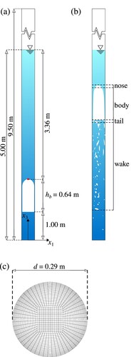
A Taylor bubble is a slug-shaped bubble of gas, raising in a vertical pipe filled with a fluid. Its behaviour depends on the gravitational acceleration, viscosity, density, surface tension and also the compressibility of the fluids (Davies & Taylor, 1950; Llewellin et al., 2012). It is usually divided in four parts: (1) a hemispherical tip called the nose, (2) a body surrounded by a film of fluid, (3) a tail region and (4) a wake, which can be laminar or turbulent. In this section, the NSLs are applied to the Taylor bubble presented in the experiments of Pringle et al. (2015) and in the numerical study of Ambrose et al. (2016). The fluid inside the bubble is compressible air surrounded by incompressible water.

Here, CFD simulations are used to validate the NSLs, i.e. between the solution at different geometrical scales with scale factors $\lambda =\frac{l_p}{l_m}$, where $l_p$ is a characteristic length in the prototype (subscript p) and $l_m$ the corresponding one in the model (subscript m).

4.2. Numerical set-up

The numerical domain consisted of a vertical cylinder of height $9.50\mathrm{m}$ with an internal diameter $d=0.29\mathrm{m}$. Initially, the pipe was filled with water to a depth of $5.00\mathrm{m}$. A bubble of air was introduced close to the bottom of the pipe by setting $\gamma =0$ in the bubble region. The initial shape of the bubble used in the numerical simulations was a hemisphere with a radius of $0.14\mathrm{m}$ on the top of a cylinder with the same radius and a height of $0.50\mathrm{m}$, resulting in a total height of $h_b=0.64\mathrm{m}$. The nose of the bubble was located at $x_3=1.64\mathrm{m}$ from the bottom of the pipe (Fig. 1). The initial pressure inside the bubble $p_0$ was set at a constant value matching the hydrostatic water pressure at the nose. The water had a constant density ${\rho }_w=1000\mathrm{k}\mathrm{g}{\mathrm{m}}^{-3}$, $\sigma =0.07\mathrm{N}{\mathrm{m}}^{-1}$ and the kinematic and dynamic viscosities were ${\nu }_w=1\times {10}^{-6}{\mathrm{m}}^2{\mathrm{s}}^{-1}$ and ${\mu }_w=1\times {10}^{-3}\mathrm{k}\mathrm{g}{\mathrm{m}}^{-1}{\mathrm{s}}^{-1}$, respectively. The initial density of air was ${\rho }_{a,0}=1\mathrm{k}\mathrm{g}{\mathrm{m}}^{-3}$, ${\nu }_a=1.48\times {10}^{-5}{\mathrm{m}}^2{\mathrm{s}}^{-1}$ and ${\mu }_a=1.48\times {10}^{-5}\mathrm{k}\mathrm{g}{\mathrm{m}}^{-1}{\mathrm{s}}^{-1}$. $T_0$ of the entire domain was set at $293\mathrm{K}$, $c_{v,w}=4195{\mathrm{m}}^2{\mathrm{K}}^{-1}{\mathrm{s}}^{-2}$ and $c_{v,a}=1007{\mathrm{m}}^2{\mathrm{K}}^{-1}{\mathrm{s}}^{-2}$.

Figure 1. Schematic illustration of the computational domain at prototype scale: (a) the longitudinal section of the domain, (b) a Taylor bubble region and (c) a cross-section of the mesh

The top boundary of the domain was modelled as a fully transmissive open boundary condition at atmospheric pressure. The no-slip boundary condition was applied to the remaining walls including the bottom. Note that, because of the orientation of the reference frame, $g_i=(0,0,-g)$ in Eq. (2(2) $\begin{array}{rl}\frac{\mathrm{\partial }\rho U_i}{\mathrm{\partial }t}+U_j\frac{\mathrm{\partial }\rho U_i}{\mathrm{\partial }{x}_j}& =\frac{\mathrm{\partial }}{\mathrm{\partial }{x}_j}(\mu \frac{\mathrm{\partial }{U}_i}{\mathrm{\partial }{x}_j}-\rho \overline{u_i{u}_j})-\frac{\mathrm{\partial }p}{\mathrm{\partial }{x}_i}+\rho g_i+f_{\sigma }\end{array}$(2) ).

A structured O-grid mesh was created with a spacing of $0.0025\mathrm{m}$ at the wall increasing to $0.0075\mathrm{m}$ at the centre (Fig. 1c) while the cells were $0.008\mathrm{m}$ tall. The mesh was refined near the wall to resolve the film around the Taylor bubble. The time step $\mathrm{\Delta }t$ was set to 0.0005 s at the start of the simulation and it was subsequently varied to respect the Courant–Friedrichs–Lewy (CFL) condition (Courant et al., 1967): (40) $\begin{array}{r}\frac{U_j\mathrm{\Delta }t}{\mathrm{\Delta }{x}_j}<C_{max}\end{array}$(40) where $\mathrm{\Delta }{x}_j$ is the mesh size in the Cartesian coordinate system in the $j\mathrm{t}\mathrm{h}$ direction ($j=1,2,3$) and $C_{max}=0.5$ is the maximum Courant number. The simulations were run on the University of Nottingham high performance computing (HPC) cluster Augusta. The number of cells in the computational domain was 1,513,200 and it required 8 h to simulate the actual time of 3.4 s by using 16 cores and 15 GB of memory (also for the corresponding times at reduced scales). All the dimensional parameters, including the mesh sizes and time steps, were scaled to the smaller domains according to the selected scaling laws.

4.3. Application of the NSLs

Three self-similar domains, namely T4, T8 and T16, were created with geometrical scale factors of $\lambda ={\text{β}}^{{\alpha }_x}=4$, 8 and 16, respectively. To achieve this, it was assumed that ${\alpha }_x=1$ such that $\text{β}=4$ (T4), 8 (T8) and 16 (T16), respectively. All variables and parameters were transformed by the scaling exponents in the sixth and seventh columns of Table 1 (with scaling conditions in terms of ${\alpha }_x$, ${\alpha }_R={\alpha }_T={\alpha }_{Mm}=0$ and ${\alpha }_n=3{\alpha }_x$). Their specific values for the prototype and the scaled models, obtained by applying the conditions in Table 2, are presented in Table 3. The prototype was also scaled by using traditional FSLs (${\mathrm{T}4}_{\mathsf{\text{F}}}$, ${\mathrm{T}8}_{\mathsf{\text{F}}}$ and ${\mathrm{T}16}_{\mathsf{\text{F}}}$) using the same λ as in the self-similar domains and by keeping the fluid properties and the temperature invariant.

Table 2. Scaling parameters and exponents used to scale the Taylor bubble prototype values to the corresponding values in the domains T4, T8 and T16 by using the NSLs

Domain	T4	T8	T16
Scaling parameter β	4	8	16
Scaling exponents
Length (m) ${\alpha }_x$	1	1	1
Time (s) ${\alpha }_t$	1	1	1
Density ($\mathrm{k}\mathrm{g}{\mathrm{m}}^{-3}$) ${\alpha }_{\rho }$	0	0	0
Velocity (m ${\mathrm{s}}^{-1}$) ${\alpha }_U$	0	0	0
Gravitational acceleration (m ${\mathrm{s}}^{-2}$) ${\alpha }_g$	$-1$	$-1$	$-1$
Pressure (Pa) ${\alpha }_p$	0	0	0
Kinematic viscosity (${\mathrm{m}}^2{\mathrm{s}}^{-1}$) ${\alpha }_{\nu }$	1	1	1
Dynamic viscosity ($\mathrm{k}\mathrm{g}{\mathrm{m}}^{-1}{\mathrm{s}}^{-1}$) ${\alpha }_{\mu }$	1	1	1
Surface tension (N ${\mathrm{m}}^{-1}){\alpha }_{\sigma }$	1	1	1
Specific heat capacity (${\mathrm{m}}^2{\mathrm{K}}^{-1}{\mathrm{s}}^{-2}$) ${\alpha }_{c_v}$	0	0	0
Scaling ratios
Length (m) ${\text{β}}^{{\alpha }_x}$	4.0000	8.0000	16.0000
Time (s) ${\text{β}}^{{\alpha }_t}$	4.0000	8.0000	16.0000
Density ($\mathrm{k}\mathrm{g}{\mathrm{m}}^{-3}$) ${\text{β}}^{{\alpha }_{\rho }}$	1.0000	1.0000	1.0000
Velocity ($\mathrm{m}{\mathrm{s}}^{-1}$) ${\text{β}}^{{\alpha }_U}$	1.0000	1.0000	1.0000
Gravitational acceleration (m ${\mathrm{s}}^{-2}$) ${\text{β}}^{{\alpha }_g}$	0.2500	0.1250	0.0625
Pressure (Pa) ${\text{β}}^{{\alpha }_p}$	1.0000	1.0000	1.0000
Kinematic viscosity (${\mathrm{m}}^2{\mathrm{s}}^{-1}$) ${\text{β}}^{{\alpha }_{\nu }}$	4.0000	8.0000	16.0000
Dynamic viscosity ($\mathrm{k}\mathrm{g}{\mathrm{m}}^{-1}{\mathrm{s}}^{-1}$) ${\text{β}}^{{\alpha }_{\mu }}$	4.0000	8.0000	16.0000
Surface tension (N ${\mathrm{m}}^{-1}$) ${\text{β}}^{{\alpha }_{\sigma }}$	4.0000	8.0000	16.0000
Specific heat capacity ($\mathrm{J}{\mathrm{k}\mathrm{g}}^{-1}{\mathrm{K}}^{-1}$) ${\text{β}}^{{\alpha }_{c_v}}$	1.0000	1.0000	1.0000

Table 3. Parameters for the Taylor bubble in the prototype and the scaled domains

Domain	T1	T4	T8	T16	${\mathrm{T}4}_{\mathsf{\text{F}}}$	${\mathrm{T}8}_{\mathsf{\text{F}}}$	${\mathrm{T}16}_{\mathsf{\text{F}}}$
Diameter of the pipe d (m)	0.290000	0.072500	0.036250	0.018125	0.072500	0.036250	0.018125
Initial height of the bubble $h_b$ (m)	0.640	0.160	0.080	0.040	0.160	0.080	0.040
Initial height of the water plug (m)	3.360	0.840	0.420	0.210	0.840	0.420	0.210
Computational time (s)	3.50000	0.87500	0.43750	0.21875	1.75000	1.23700	0.87500
Gravitational acceleration g (m ${\mathrm{s}}^{-2}$)	9.81	39.24	78.48	156.96	9.81	9.81	9.81
Initial pressure inside the bubble $p_0$ (Pa)	134286.000	134286.000	134286.000	134286.000	33571.500	16785.750	8392.875
Density of water ${\rho }_w$ (kg ${\mathrm{m}}^{-3}$)	1000	1000	1000	1000	1000	1000	1000
Initial density of air ${\rho }_{a,0}$ (kg ${\mathrm{m}}^{-3}$)	1	1	1	1	1	1	1
Kinematic viscosity of water ${\nu }_w$ (${\mathrm{m}}^2{\mathrm{s}}^{-1}$)	$1\times {10}^{-6}$	$2.50\times {10}^{-7}$	$1.25\times {10}^{-7}$	$6.25\times {10}^{-8}$	$1\times {10}^{-6}$	$1\times {10}^{-6}$	$1\times {10}^{-6}$
Dynamic viscosity of water ${\mu }_w$ ($\mathrm{k}\mathrm{g}{\mathrm{m}}^{-1}{\mathrm{s}}^{-1}$)	$1\times {10}^{-3}$	$2.50\times {10}^{-4}$	$1.25\times {10}^{-4}$	$6.25\times {10}^{-5}$	$1\times {10}^{-3}$	$1\times {10}^{-3}$	$1\times {10}^{-3}$
Surface tension σ (N ${\mathrm{m}}^{-1}$)	0.07	$1.75\times {10}^{-2}$	$8.75\times {10}^{-3}$	$4.38\times {10}^{-3}$	0.07	0.07	0.07
Specific heat capacity of water $c_{v,w}$ ($\mathrm{J}{\mathrm{k}\mathrm{g}}^{-1}{\mathrm{K}}^{-1}$)	4195	4195	4195	4195	4195	4195	4195
Specific heat capacity of air $c_{v,a}$ ($\mathrm{J}{\mathrm{k}\mathrm{g}}^{-1}{\mathrm{K}}^{-1}$)	1007	1007	1007	1007	1007	1007	1007
Initial temperature $T_0$ (K)	293	293	293	293	293	293	293

4.4. Results and discussion

The numerical simulation of the prototype overestimates the rise velocity of the Taylor bubble presented in Pringle et al. (2015) by approximately 40% with a dimensionless velocity $U_b^{\prime }=U_b/\sqrt{gd}=0.486$, where $U_b$ is the velocity magnitude of the bubble nose. This difference is due to the errors introduced in the numerical simulations (Ambrose et al., 2016). It is worth mentioning that the differences to the experimental results do not affect the validation of the NSLs as the validation is based on comparing the results of T1 with the ones from the scaled domains.

Nevertheless, the general behaviour of the Taylor bubble agrees qualitatively with the experimental findings of Pringle et al. (2015). The bubble transits to its stable shape between dimensionless time $t^{\prime }=t\sqrt{g/d}=0$ and 6 in the prototype. After $t^{\prime }=6$, the slug shaped bubble fully forms, rising with a constant $U_b^{\prime }$.

The initial stage of bubble formation is illustrated in Fig. 2, showing the cross-section $x_2^{\prime }=x_2/d=0$ at $t^{\prime }=2.90$ of T1, T16 and $\mathrm{T}{16}_{\mathsf{\text{F}}}$. Both T1 and T16 show the bubble divided by the water. Note that the details of the air bubbles differ between T1 and T16; however, the dynamics of the transition of the bubble to the final shape is the same. This means that self-similarity at the scale of individual bubbles with dimensions much smaller than the Taylor bubble is not expected. In $\mathrm{T}{16}_{\mathsf{\text{F}}}$, a slug-shape bubble is formed with a very limited wake and smaller bubbles.

Figure 2. Snapshot of the Taylor bubble at the cross-section $x_2^{\prime }=0$ and dimensionless time $t^{\prime }=2.90$ of (a) the prototype, (b) T16 and (c) ${\mathrm{T}16}_{\mathsf{\text{F}}}$

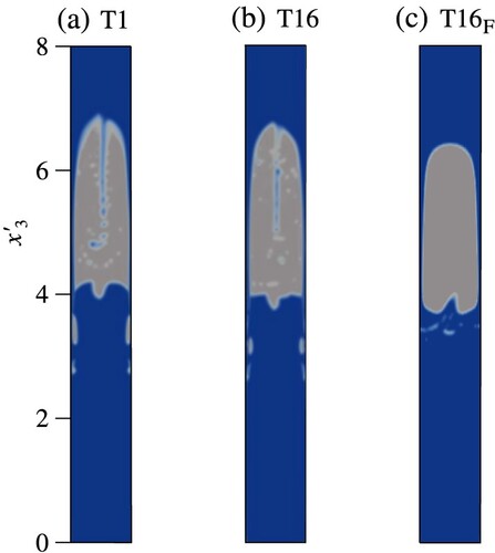
Figure 3 shows the cross-sections $x_2^{\prime }=0$ of the domains at $t^{\prime }=14.54$ for T1, T16 and ${\mathrm{T}16}_{\mathsf{\text{F}}}$. The prototype and T16 show the typical slug shape with the nose situated almost at $x_3^{\prime }=x_3/d=13$. This suggests that there is no scale effect for $U_b$ by using the NSLs. Further, the shedding of smaller bubbles can be seen in the wake of the main one. In the domain scaled with the traditional FSLs the behaviour is significantly different. Indeed, the nose is rounder with respect to T1 and the nose reaches $x_3^{\prime }=10$. Moreover, the wake contains less air along the $x_3^{\prime }$ axis.

Figure 3. Snapshot of the Taylor bubble at the cross-section $x_2^{\prime }=0$ and dimensionless time $t^{\prime }=14.54$ of (a) the prototype, (b) T16 and (c) ${\mathrm{T}16}_{\mathsf{\text{F}}}$

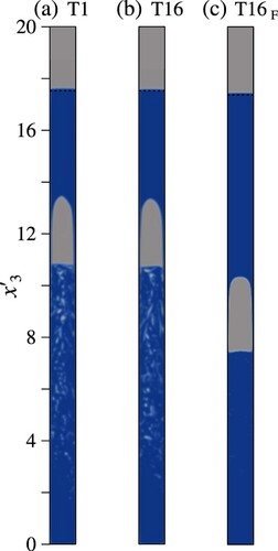
Figure 4 shows the time history of the $x_3^{\prime }$ position of the nose. The slopes of the curves represent $U_b^{\prime }$. $U_b^{\prime }$ is computed after $t^{\prime }=6$, i.e. after the initial stage in which the bubble shape is unstable. As shown in Table 4, $U_b^{\prime }$ for T4, T8 and T16 are nearly self-similar with respect to the prototype. Table 4 shows also the relative differences of $U_b^{\prime }$ computed as: (41) $\begin{array}{r}{E}_{U_b^{\prime }}=100\frac{|U_{b,p}^{\prime }-U_{b,m}^{\prime }|}{U_{b,p}^{\prime }}\end{array}$(41) where $U_{b,p}^{\prime }$ is the value of $U_b^{\prime }$ in the prototype and $U_{b,m}^{\prime }$ in the scaled domains. The small differences between the prototype and the models scaled with the NSLs are also confirmed in Fig. 4, where the respective curves do not overlap. 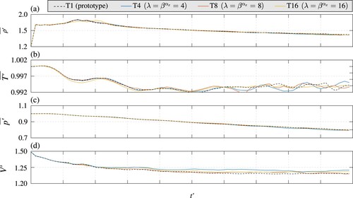Nevertheless, the differences are not directly proportional to λ, as also shown by $E_{U_b^{\prime }}$, which is even smaller in T16 than in T4 and T8 (Table 4). Hence, there is no evidence that those differences are related to the increase of λ, i.e. due to scale effects. In contrast, by using the traditional FSLs there is a clear demonstration of scale effects. Indeed, $E_{U_b^{\prime }}$ increases with increasing λ, reaching 30.66% in ${\mathrm{T}16}_{\mathsf{\text{F}}}$.

Figure 4. Time history of the bubble nose location on the $x_3^{\prime }$ coordinate for the prototype and all the scaled domains

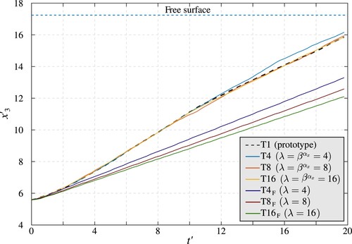
Table 4. $U_b^{\prime }$ for the prototype and all scaled domains

	T1	T4	T8	T16	${\mathrm{T}4}_{\mathsf{\text{F}}}$	${\mathrm{T}8}_{\mathsf{\text{F}}}$	${\mathrm{T}16}_{\mathsf{\text{F}}}$
$U_b^{\prime }$	0.486	0.476	0.495	0.482	0.398	0.363	0.337
$E_{U_b^{\prime }}$ (%)	–	2.06	1.85	0.82	18.11	25.31	30.66

It is relevant to analyse whether the NSLs guarantee self-similarity with respect to Eq. (7(7) $\begin{array}{r}nT=\frac{pV}{R_u}\end{array}$(7) ). Figure 5 shows the time histories of the averages of the dimensionless densities $\overline{{\rho }^{\prime }}=\overline{\rho }/{\rho }_{a,0}$, temperatures $\overline{T^{\prime }}=\overline{T}/T_0$ and pressures $\overline{p^{\prime }}=\overline{p}/p_0$ inside the bubbles as well as the variation of the corresponding dimensionless volumes $V^{\prime }=V/d^3$, for the self-similar domains. The prototype T1, T4, T8 and T16 show a sudden increase in $\overline{{\rho }^{\prime }}$ and from $t^{\prime }=6$, $\overline{{\rho }^{\prime }}$ decrease almost linearly. This is due to the transitory stage in which the bubble is suddenly compressed (Fig. 2). In the prototype, $\overline{T^{\prime }}$ consistently decreases with some fluctuations. This behaviour is also replicated in T4, T8 and T16, even if the curves do not perfectly overlap. The differences in $\overline{T^{\prime }}$ between the prototype and the scaled domains are less than $\pm 0.005$ such that they do not indicate significant scale effects. $\overline{p^{\prime }}$ matches between the prototype and the self-similar domains, decreasing linearly with the ascent of the bubble. Furthermore, the volume of the bubble $V^{\prime }$ confirms self-similarity between T1, T4, T8 and T16.

Figure 5. Time histories of the averages of (a) the dimensionless density $\overline{{\rho }^{\prime }}$, (b) the dimensionless temperature $\overline{T^{\prime }}$ and (c) the dimensionless pressure $\overline{p^{\prime }}$ inside each modelled Taylor bubble and (d) the dimensionless volume $V^{\prime }$ for T1, T4, T8 and T16

The time histories of $\overline{{\rho }^{\prime }}$, $\overline{T^{\prime }}$, $\overline{p^{\prime }}$ and $V^{\prime }$ for the domains scaled with the traditional FSLs are presented in Fig. 6. In contrast to the NSLs, ${\mathrm{T}4}_{\mathsf{\text{F}}}$, ${\mathrm{T}8}_{\mathsf{\text{F}}}$ and ${\mathrm{T}16}_{\mathsf{\text{F}}}$ fail to reproduce the behaviour of the prototype and the time series of the aforementioned variables are completely different from those of the prototype and those obtained with the NSLs. Indeed, $\overline{{\rho }^{\prime }}$ decreases and remains constant from $t^{\prime }=0.5$ until the end of the simulation.

Figure 6. Time histories of the averages of the (a) dimensionless density $\overline{{\rho }^{\prime }}$, (b) dimensionless temperature $\overline{T^{\prime }}$ and (c) dimensionless pressure $\overline{p^{\prime }}$ inside the bubbles and (d) the dimensionless volume $V^{\prime }$ for T1, ${\mathrm{T}4}_{\mathsf{\text{F}}}$, ${\mathrm{T}8}_{\mathsf{\text{F}}}$ and ${\mathrm{T}16}_{\mathsf{\text{F}}}$

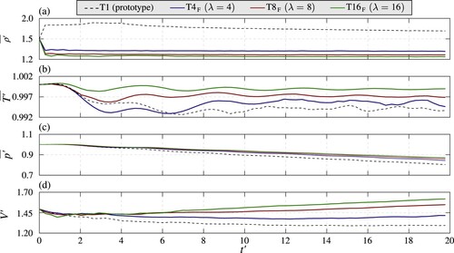
Since the traditional FSLs overestimate the viscosity and the surface tension and do not account for the air compressibility, the bubble is not compressed at the beginning of the simulations, and the initial variation of $V^{\prime }$ is smaller (Fig. 6c). Consequently, $\overline{{\rho }^{\prime }}$ decreases suddenly in contrast to the prototype. The overestimation of the pressure effects is demonstrated in Fig. 6c, showing the variation in the slope of $\overline{p^{\prime }}$ with increasing λ. Both the absolute and relative fluctuations of $\overline{T^{\prime }}$ reduce with increasing λ. Finally, in ${\mathrm{T}4}_{\mathsf{\text{F}}}$, ${\mathrm{T}8}_{\mathsf{\text{F}}}$ and ${\mathrm{T}16}_{\mathsf{\text{F}}}$, $V^{\prime }$ increases in time and its maximum value increases also with λ. Hence, the traditional FSLs introduce scale effects, which increase with λ.

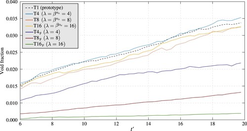
When the bubble rises, the pressure decreases such that the bubble expands, while also releasing air into the wake and $V^{\prime }$ decreases. This occurs in the prototype and in the self-similar domains. Hence, domains T1, T4, T8 and T16 have more air in the wake with respect to the domains scaled with traditional FSLs (Fig. 3). This behaviour is clearly demonstrated in Fig. 7 showing the time history of the void fraction in the wake, namely the volume of air in the wake divided by the volume of the entire domain between the bottom and the free surface. It is worth mentioning that the void fraction depends on the viscosity, surface tension and the compressibility of the bubble that in turn is related to the heat exchange between water and air. Hence, the same amount of void fraction behind the bubbles shows that all these effects are scaled correctly. The behaviour in the domains T1, T4, T8 and T16 is the same, having a void fraction around 0.035 at the end of the simulation. The differences between the self-similar domains may be due to the small differences in describing individual bubbles at scales smaller than the Taylor one, as shown in the initial stages of the motion in Fig. 2. Nevertheless, the general behaviour of the Taylor bubble is scaled in T4, T8 and T16 with differences that are not associated with scale effects, since they are not directly proportional to λ, in contrast to the differences observed in domains ${\mathrm{T}4}_{\mathsf{\text{F}}}$, ${\mathrm{T}8}_{\mathsf{\text{F}}}$ and ${\mathrm{T}16}_{\mathsf{\text{F}}}$. Indeed, the viscosity and surface tension are overestimated and the compressibility of air and the related heat exchange are neglected.

Figure 7. Time history of the void fraction lost in the wake of the bubble for the prototype and the scaled domains

5. Conclusions

The Froude scaling laws (FSLs) have been applied to air–water flows at reduced size for almost a century. A significant disadvantage of this scaling approach is the introduction of scale effects due to the overestimation of the viscosity and surface tension. Furthermore, the compressibility of air and heat exchange are neglected, thus additional scale effects are potentially introduced. In this article, Lie group transformations are applied to the system of governing equations of compressible air–water flows to derive novel scaling laws (NSLs), allowing the modelling of hydrodynamic phenomena at small scales without viscous, surface tension, compressibility and heat exchange scale effects.

Since the temperature cannot be reduced below the freezing point and the molar mass as well as the molar density need to be the same, some restrictions on the scaling exponents are taken into account. Hence, the scaling configuration used in this work is expressed as a function of the scaling exponents of the length ${\alpha }_x$, the specific gas constant ${\alpha }_R$, the temperature ${\alpha }_T$, the molar mass ${\alpha }_{Mm}$ and the number of moles ${\alpha }_n$.

The derived NSLs were validated numerically with the simulation of a Taylor bubble. Computational fluid dynamics simulations allow for testing a wide range of conditions, including domain T16, where the model size was relatively small. The results show that the general behaviour of the phenomenon is correctly scaled. The small differences observed between the models and the prototype are not due to scale effects but the divergences in describing the motion of individual bubbles that have dimensions much smaller than the Taylor one. In contrast, the FSLs introduce scale effects proportional to the geometrical scale factor, showing a distinct behaviour with respect to the prototype and those obtained with the NSLs.

An advantage of this novel scaling method is that it uses the system of governing equations of the phenomenon and it provides a complete picture of the conditions that all the parameters and variables involved must satisfy to obtain self-similarity. Hence, the NSLs are more general than the FSLs based on the hypothesis that the viscosity, surface tension, compressibility of air and heat exchange are unscaled.

The scaling configuration proposed implies that the gravitational acceleration g needs to be increased in the model, since its scaling exponent is negative (${\alpha }_g=-{\alpha }_x$). This can be done in the laboratory by conducting centrifuge model tests (e.g. Zhang et al., 2009). Alternatively, future works can focus on finding other scaling configurations, e.g. the application of Lie group transformations to compressible air–water flows under adiabatic conditions.

Notation

$C_{\mathrm{m}\mathrm{a}\mathrm{x}}$	=	maximum Courant number (–)
$C_{ϵ1}$, $C_{ϵ2}$, $C_{\mu }$, $C_{{\sigma }_k}$ and $C_{{\sigma }_{ϵ}}$	=	standard coefficients used in the k-ϵ model (–)
$c_v$	=	specific heat capacity (m${}^2$ K${}^{-1}$ s${}^{-2}$)
d	=	bubble diameter (m)
$E_{U_b^{\prime }}$	=	relative differences in the Taylor bubble velocity (
$f_{\sigma }$	=	surface tension force (N)
F	=	Froude number (–)
$g_i$	=	gravitational acceleration (m s${}^{-2}$)
$h_b$	=	initial height of the bubble (m)
k	=	turbulence kinetic energy (m${}^2$ s${}^{-2}$)
l	=	characteristic length (m)
$M_c$	=	molar density (mol m${}^{-3}$)
$M_m$	=	molar mass (kg mol${}^{-1}$)
n	=	number of moles (mol)
N	=	number of specific elementary entities (–)
$N_A$	=	Avogadro number (–)
p	=	Reynolds-averaged pressure (Pa)
$\overline{p^{\prime }}$	=	average of the dimensionless pressure inside the Taylor bubble (–)
$p_0$	=	initial pressure inside the Taylor bubble (Pa)
$P_k$	=	Production of turbulence due to horizontal velocity gradients (m${}^2$ s${}^{-3}$)
R	=	Reynolds number (–)
R	=	specific gas constant (m${}^2$ K${}^{-1}$ s${}^{-2}$)
$R_u$	=	ideal gas constant (J mol${}^{-1}$ K${}^{-1}$)
T	=	temperature (K)
$\overline{T^{\prime }}$	=	average of the dimensionless temperature inside the Taylor bubble (–)
$T_0$	=	initial temperature inside the Taylor bubble (–)
t	=	time (s)
$t^{\prime }$	=	dimensionless time (–)
$U_b$	=	velocity of the Taylor bubble (m s${}^{-1}$)
$U_b^{\prime }$	=	dimensionless velocity of the Taylor bubble (–)
U	=	Reynolds-averaged flow velocity components (m s${}^{-1}$)
$U^{\prime }$	=	dimensionless Reynolds-averaged flow velocity components (–)
u	=	fluctuating velocity components (m s${}^{-1}$)
$\overline{u_{\mathrm{i}}{u}_{\mathrm{j}}}$	=	Reynolds stress term (m${}^2$ s${}^{-2}$)
V	=	air volume (m${}^3$)
$V^{\prime }$	=	dimensionless air volume (–)
W	=	Weber number (–)
x	=	spatial coordinates (m)
$x^{\prime }$	=	dimensionless spatial coordinates (–)
${\alpha }_{c,v}$	=	scaling exponent for the specific heat capacity (–)
${\alpha }_{f_{\sigma }}$	=	scaling exponent for the surface tension force (–)
${\alpha }_g$	=	scaling exponent for the gravitational acceleration (–)
${\alpha }_k$	=	scaling exponent for the turbulence kinetic energy (–)
${\alpha }_{M_m}$	=	scaling exponent for the molar mass (–)
${\alpha }_n$	=	scaling exponent for the number of mole (–)
${\alpha }_p$	=	scaling exponent for the pressure (–)
${\alpha }_{P_k}$	=	scaling exponent for the production of turbulence due to horizontal velocity gradients (–)
${\alpha }_R$	=	scaling exponent for the specific gas constant (–)
${\alpha }_T$	=	scaling exponent for the temperature (–)
${\alpha }_t$	=	scaling exponent of the time (–)
${\alpha }_U$	=	scaling exponent for the velocity (–)
${\alpha }_u$	=	scaling exponent for the velocity fluctuation (–)
${\alpha }_{\overline{u_{\mathrm{i}}{u}_{\mathrm{j}}}}$	=	scaling exponent for the Reynolds stress term (–)
${\alpha }_x$	=	scaling exponent of the length (–)
${\alpha }_{ϵ}$	=	scaling exponent for the dissipation of the turbulent kinetic energy (–)
${\alpha }_{\kappa }$	=	scaling exponent for the curvature of the free surface (–)
${\alpha }_{\mu }$	=	scaling exponent for the dynamic viscosity (–)
${\alpha }_{\nu }$	=	scaling exponent for the kinematic viscosity (–)
${\alpha }_{{\nu }_t}$	=	scaling exponent for the eddy viscosity (–)
${\alpha }_{\rho }$	=	scaling exponent for the density (–)
${\alpha }_{\sigma }$	=	scaling exponent for the surface tension (–)
${\alpha }_{\varphi }$	=	scaling exponent of ϕ (–)
β	=	scaling parameter (–)
γ	=	phase fraction (–)
$\mathrm{\Delta }t$	=	time step (s)
$\mathrm{\Delta }x$	=	mesh size (m)
${\delta }_{\mathrm{i}\mathrm{j}}$	=	Kronecker delta (–)
ϵ	=	rate of dissipation of the turbulent kinetic energy (m${}^2$ s${}^{-3}$)
κ	=	curvature of the free surface (m${}^{-1}$)
λ	=	geometrical scale factor (–)
μ	=	dynamic viscosity ( kg m${}^{-1}$ s${}^{-1}$)
ν	=	kinematic viscosity (m${}^2$ s${}^{-1}$)
${\nu }_t$	=	eddy viscosity (m${}^2$ s${}^{-1}$)
ρ	=	density (kg m${}^{-3}$)
${\rho }^{\prime }$	=	initial dimensionless density of air inside the Taylor bubble (–)
$\overline{{\rho }^{\prime }}$	=	average of the dimensionless density inside the Taylor bubble (kg m${}^{-3}$)
σ	=	surface tension (N m${}^{-1}$)
ϕ	=	variable in the original space (various)
$\varphi \ast$	=	variable in the transformed space (various)

Subscripts

a	=	air
F	=	Froude
i	=	free index
j	=	dummy index
m	=	model
p	=	prototype
$U^{\prime }$	=	dimensionless velocity (–)
w	=	water

Acknowledgments

The authors would like to thank Dr David Hargreaves for helpful suggestions. The simulations were conducted on the University of Nottingham HPC clusters Augusta.

Disclosure statement

No potential conflict of interest was reported by the author(s).

Additional information

Funding

The work was carried out as part of Daniele Catucci's PhD study, funded by the University of Nottingham Pro-Vice Chancellor Research Excellence Scholarship.

Appendix A

The Lie group transformations for Eq. (1(1) $\begin{array}{rl}\frac{\mathrm{\partial }\rho }{\mathrm{\partial }t}+\frac{\mathrm{\partial }\rho U_j}{\mathrm{\partial }{x}_j}& =0,\end{array}$(1) ) yield the following equations in the transformed domain: (A1) $\begin{array}{r}{\text{β}}^{{\alpha }_{\rho }-{\alpha }_t}\frac{\mathrm{\partial }{\rho }^{\ast }}{\mathrm{\partial }{t}^{\ast }}+{\text{β}}^{{\alpha }_{\rho }+{\alpha }_U-{\alpha }_x}\frac{\mathrm{\partial }{\rho }^{\ast }{U}_j^{\ast }}{\mathrm{\partial }{x}_j^{\ast }}=0\end{array}$(A1) Self-similarity is guaranteed if the scaling ratios of all terms in Eq. (A1(A1) $\begin{array}{r}{\text{β}}^{{\alpha }_{\rho }-{\alpha }_t}\frac{\mathrm{\partial }{\rho }^{\ast }}{\mathrm{\partial }{t}^{\ast }}+{\text{β}}^{{\alpha }_{\rho }+{\alpha }_U-{\alpha }_x}\frac{\mathrm{\partial }{\rho }^{\ast }{U}_j^{\ast }}{\mathrm{\partial }{x}_j^{\ast }}=0\end{array}$(A1) ) are the same, implying that the exponents of all terms must also be the same: (A2) $\begin{array}{r}{\alpha }_{\rho }-{\alpha }_t={\alpha }_{\rho }+{\alpha }_U-{\alpha }_x\Rightarrow {\alpha }_U={\alpha }_x-{\alpha }_t\end{array}$(A2) This confirms that the scaling condition for the velocity is the same as for incompressible flows in Catucci et al. (2021).

The Lie group transformations for Eq. (2(2) $\begin{array}{rl}\frac{\mathrm{\partial }\rho U_i}{\mathrm{\partial }t}+U_j\frac{\mathrm{\partial }\rho U_i}{\mathrm{\partial }{x}_j}& =\frac{\mathrm{\partial }}{\mathrm{\partial }{x}_j}(\mu \frac{\mathrm{\partial }{U}_i}{\mathrm{\partial }{x}_j}-\rho \overline{u_i{u}_j})-\frac{\mathrm{\partial }p}{\mathrm{\partial }{x}_i}+\rho g_i+f_{\sigma }\end{array}$(2) ) yield the following equation in the transformed domain: (A3) $\begin{array}{rl}& {\text{β}}^{{\alpha }_{\rho }+{\alpha }_U-{\alpha }_t}\frac{\mathrm{\partial }{\rho }^{\ast }{U}_i^{\ast }}{\mathrm{\partial }{t}^{\ast }}+{\text{β}}^{2{\alpha }_U+{\alpha }_{\rho }-{\alpha }_x}{U}_j^{\ast }\frac{\mathrm{\partial }{\rho }^{\ast }{U}_i^{\ast }}{\mathrm{\partial }{x}_j^{\ast }}\\ & ={\text{β}}^{{\alpha }_{\mu }+{\alpha }_U-2{\alpha }_x}\frac{\mathrm{\partial }}{\mathrm{\partial }{x}_j^{\ast }}\left({\mu }^{\ast }\frac{\mathrm{\partial }{U}_i^{\ast }}{\mathrm{\partial }{x}_j^{\ast }}\right)-{\text{β}}^{{\alpha }_{\rho }+{\alpha }_{\overline{uu}}-{\alpha }_x}\frac{\mathrm{\partial }}{\mathrm{\partial }{x}_j^{\ast }}\left({\rho }^{\ast }\overline{u_i^{\ast }{u}_j^{\ast }}\right)\\ & -{\text{β}}^{{\alpha }_p-{\alpha }_x}\frac{\mathrm{\partial }{p}^{\ast }}{\mathrm{\partial }{x}_j^{\ast }}+{\text{β}}^{{\alpha }_{\rho }+{\alpha }_g}{\rho }^{\ast }{g}_i^{\ast }+{\text{β}}^{{\alpha }_{f_{\sigma }}}{f}_{\sigma }^{\ast }\end{array}$(A3) Equation (A3(A3) $\begin{array}{rl}& {\text{β}}^{{\alpha }_{\rho }+{\alpha }_U-{\alpha }_t}\frac{\mathrm{\partial }{\rho }^{\ast }{U}_i^{\ast }}{\mathrm{\partial }{t}^{\ast }}+{\text{β}}^{2{\alpha }_U+{\alpha }_{\rho }-{\alpha }_x}{U}_j^{\ast }\frac{\mathrm{\partial }{\rho }^{\ast }{U}_i^{\ast }}{\mathrm{\partial }{x}_j^{\ast }}\\ & ={\text{β}}^{{\alpha }_{\mu }+{\alpha }_U-2{\alpha }_x}\frac{\mathrm{\partial }}{\mathrm{\partial }{x}_j^{\ast }}\left({\mu }^{\ast }\frac{\mathrm{\partial }{U}_i^{\ast }}{\mathrm{\partial }{x}_j^{\ast }}\right)-{\text{β}}^{{\alpha }_{\rho }+{\alpha }_{\overline{uu}}-{\alpha }_x}\frac{\mathrm{\partial }}{\mathrm{\partial }{x}_j^{\ast }}\left({\rho }^{\ast }\overline{u_i^{\ast }{u}_j^{\ast }}\right)\\ & -{\text{β}}^{{\alpha }_p-{\alpha }_x}\frac{\mathrm{\partial }{p}^{\ast }}{\mathrm{\partial }{x}_j^{\ast }}+{\text{β}}^{{\alpha }_{\rho }+{\alpha }_g}{\rho }^{\ast }{g}_i^{\ast }+{\text{β}}^{{\alpha }_{f_{\sigma }}}{f}_{\sigma }^{\ast }\end{array}$(A3) ) is self-similar if: (A4) $\begin{array}{rl}{\alpha }_{\rho }+{\alpha }_U-{\alpha }_t& =2{\alpha }_U+{\alpha }_{\rho }-{\alpha }_x\\ & ={\alpha }_{\mu }+{\alpha }_U-2{\alpha }_x\\ & ={\alpha }_{\rho }+{\alpha }_{\overline{uu}}-{\alpha }_x\\ & ={\alpha }_p-{\alpha }_x\\ & ={\alpha }_{\rho }+{\alpha }_g\\ & ={\alpha }_{f_{\sigma }}\end{array}$(A4) From Eq. (A4(A4) $\begin{array}{rl}{\alpha }_{\rho }+{\alpha }_U-{\alpha }_t& =2{\alpha }_U+{\alpha }_{\rho }-{\alpha }_x\\ & ={\alpha }_{\mu }+{\alpha }_U-2{\alpha }_x\\ & ={\alpha }_{\rho }+{\alpha }_{\overline{uu}}-{\alpha }_x\\ & ={\alpha }_p-{\alpha }_x\\ & ={\alpha }_{\rho }+{\alpha }_g\\ & ={\alpha }_{f_{\sigma }}\end{array}$(A4) ) the scaling exponent of μ is obtained as: (A5) $\begin{array}{r}{\alpha }_{\rho }+{\alpha }_U-{\alpha }_t={\alpha }_{\mu }+{\alpha }_U-2{\alpha }_x\Rightarrow {\alpha }_{\mu }={\alpha }_{\rho }+2{\alpha }_x-{\alpha }_t\end{array}$(A5) The Lie group transformations for Eq. (3(3) $\begin{array}{r}{f}_{\sigma }=\sigma \kappa \frac{\mathrm{\partial }\gamma }{\mathrm{\partial }{x}_i}\end{array}$(3) ) result in: (A6) $\begin{array}{r}{\text{β}}^{{\alpha }_{f_{\sigma }}}{f}_{\sigma }^{\ast }={\text{β}}^{{\alpha }_{\sigma }+{\alpha }_{\kappa }+{\alpha }_{\gamma }-{\alpha }_{x_i}}{\sigma }^{\ast }{\kappa }^{\ast }\frac{\mathrm{\partial }{\gamma }^{\ast }}{\mathrm{\partial }{x}_i^{\ast }}\end{array}$(A6) The dimension of κ is the inverse of a length such that ${\alpha }_{\kappa }=-{\alpha }_{x_i}$. Further, ${\alpha }_{\gamma }=0$ because γ is dimensionless. Hence, Eq. (A6(A6) $\begin{array}{r}{\text{β}}^{{\alpha }_{f_{\sigma }}}{f}_{\sigma }^{\ast }={\text{β}}^{{\alpha }_{\sigma }+{\alpha }_{\kappa }+{\alpha }_{\gamma }-{\alpha }_{x_i}}{\sigma }^{\ast }{\kappa }^{\ast }\frac{\mathrm{\partial }{\gamma }^{\ast }}{\mathrm{\partial }{x}_i^{\ast }}\end{array}$(A6) ) reduces to: (A7) $\begin{array}{r}{\alpha }_{f_{\sigma }}={\alpha }_{\sigma }-2{\alpha }_{x_i}\end{array}$(A7) ${\alpha }_g$, ${\alpha }_p$ and ${\alpha }_{\nu }$ are obtained from Eq. (A4(A4) $\begin{array}{rl}{\alpha }_{\rho }+{\alpha }_U-{\alpha }_t& =2{\alpha }_U+{\alpha }_{\rho }-{\alpha }_x\\ & ={\alpha }_{\mu }+{\alpha }_U-2{\alpha }_x\\ & ={\alpha }_{\rho }+{\alpha }_{\overline{uu}}-{\alpha }_x\\ & ={\alpha }_p-{\alpha }_x\\ & ={\alpha }_{\rho }+{\alpha }_g\\ & ={\alpha }_{f_{\sigma }}\end{array}$(A4) ) and they can be written in terms of ${\alpha }_x$, ${\alpha }_t$ and ${\alpha }_{\rho }$ as: (A8) $\begin{array}{rl}& {\alpha }_{\rho }+{\alpha }_U-{\alpha }_t={\alpha }_{\rho }+{\alpha }_g\Rightarrow {\alpha }_g={\alpha }_x-2{\alpha }_t\end{array}$(A8) (A9) $\begin{array}{rl}& {\alpha }_{\rho }+{\alpha }_U-{\alpha }_t={\alpha }_p-{\alpha }_x\Rightarrow {\alpha }_p=2{\alpha }_x-2{\alpha }_t+{\alpha }_{\rho }\end{array}$(A9) By using Eqs (A4(A4) $\begin{array}{rl}{\alpha }_{\rho }+{\alpha }_U-{\alpha }_t& =2{\alpha }_U+{\alpha }_{\rho }-{\alpha }_x\\ & ={\alpha }_{\mu }+{\alpha }_U-2{\alpha }_x\\ & ={\alpha }_{\rho }+{\alpha }_{\overline{uu}}-{\alpha }_x\\ & ={\alpha }_p-{\alpha }_x\\ & ={\alpha }_{\rho }+{\alpha }_g\\ & ={\alpha }_{f_{\sigma }}\end{array}$(A4) ) and (A7(A7) $\begin{array}{r}{\alpha }_{f_{\sigma }}={\alpha }_{\sigma }-2{\alpha }_{x_i}\end{array}$(A7) ): (A10) $\begin{array}{r}{\alpha }_U-{\alpha }_t={\alpha }_{f_{\sigma }}-{\alpha }_{\rho }\Rightarrow {\alpha }_x-2{\alpha }_t={\alpha }_{\sigma }-2{\alpha }_x-{\alpha }_{\rho }\end{array}$(A10) from which: (A11) $\begin{array}{r}{\alpha }_{\sigma }=3{\alpha }_x-2{\alpha }_t+{\alpha }_{\rho }\end{array}$(A11) Similarly, the application of the Lie group transformations to Eqs (8(8) $\begin{array}{r}-\overline{u_i{u}_j}={\nu }_t(\frac{\mathrm{\partial }{U}_i}{\mathrm{\partial }{x}_j}+\frac{\mathrm{\partial }{U}_j}{\mathrm{\partial }{x}_i})-2/3k{\delta }_{ij}\end{array}$(8) )–(11(11) $\begin{array}{rl}\frac{\mathrm{\partial }ϵ}{\mathrm{\partial }t}+U_j\frac{\mathrm{\partial }ϵ}{\mathrm{\partial }{x}_j}& =C_{ϵ1}\frac{ϵ}{k}{P}_k-C_{ϵ2}\frac{{ϵ}^2}{k}\\ & +\frac{\mathrm{\partial }}{\mathrm{\partial }{x}_j}\left[\right(\nu +{\nu }_t/C_{{\sigma }_{ϵ}}\left)\frac{\mathrm{\partial }ϵ}{\mathrm{\partial }{x}_j}\right]\end{array}$(11) ) are reported in Catucci et al. (2021) with the derivation of ${\alpha }_{{\nu }_t}$, ${\alpha }_k$, ${\alpha }_{ϵ}$ and ${\alpha }_{P_k}$.

References

- Ambrose, S., Hargreaves, D. M., & Lowndes, I. S. (2016). Numerical modeling of oscillating Taylor bubbles. Engineering Applications of Computational Fluid Mechanics, 10(1), 578–598. https://doi.org/10.1080/19942060.2016.1224737
- Analytical Methods Committee AMCAN86 (2019). Revision of the international system of units (background paper). Royal Society of Chemistry, 11(12), 1577–1579. https://doi.org/10.1039/C9AY90028D
- Bagnold, R. A. (1939). Interim report on wave-pressure research. Journal of the Institution of Civil Engineers, 12(7), 202–226. https://doi.org/10.1680/ijoti.1939.14539
- Barenblatt, G. I. (2003). Scaling (Vol. 34). Cambridge University Press.
- Brackbill, J. U., Kothe, D. B., & Zemach, C. (1992). A continuum method for modeling surface tension. Journal of Computational Physics, 100(2), 335–354. https://doi.org/10.1016/0021-9991(92)90240-Y
- Bredmose, H., Bullock, G., & Hogg, A. (2015). Violent breaking wave impacts. Part 3. Effects of scale and aeration. Journal of Fluid Mechanics, 765, 82–113. https://doi.org/10.1017/jfm.2014.692
- Carr, K. J., Ercan, A., & Kavvas, M. L. (2015). Scaling and self-similarity of one-dimensional unsteady suspended sediment transport with emphasis on unscaled sediment material properties. Journal of Hydraulic Engineering, 141(5), Article 04015003. https://doi.org/10.1061/(ASCE)HY.1943-7900.0000994
- Catucci, D., Briganti, R., & Heller, V. (2021). Numerical validation of novel scaling laws for air entrainment in water. Proceedings of the Royal Society A: Mathematical, Physical and Engineering Sciences, 477(2255), Article 20210339. https://doi.org/10.1098/rspa.2021.0339
- Catucci, D., Briganti, R., & Heller, V. (2022). Analytical and numerical study of novel scaling laws for air-water flows. In Proceeding of the 39th IAHR World Congress, 4551–4560.
- Chanson, H., Aoki, S., & Hoque, A. (2004). Physical modelling and similitude of air bubble entrainment at vertical circular plunging jets. Chemical Engineering Science, 59(4), 747–758. https://doi.org/10.1016/j.ces.2003.11.016
- Chouet, B., Saccorotti, G., Martini, M., Dawson, P., De Luca, G., Milana, G., & Scarpa, R. (1997). Source and path effects in the wave fields of tremor and explosions at Stromboli volcano, Italy. Journal of Geophysical Research: Solid Earth, 102(B7), 15129–15150. https://doi.org/10.1029/97JB00953
- Courant, R., Friedrichs, K., & Lewy, H. (1967). On the partial difference equations of mathematical physics. IBM Journal of Research and Development, 11(2), 215–234. https://doi.org/10.1147/rd.112.0215
- Davies, R. M., & Taylor, G. I. (1950). The mechanics of large bubbles rising through extended liquids and through liquids in tubes. Proceedings of the Royal Society of London. Series A. Mathematical and Physical Sciences, 200(1062), 375–390. https://doi.org/10.1098/rspa.1950.0023
- Ercan, A., & Kavvas, M. L. (2015). Self-similarity in incompressible Navier-Stokes equations. Chaos: An Interdisciplinary Journal of Nonlinear Science, 25(12), Article 123126. https://doi.org/10.1063/1.4938762
- Ercan, A., & Kavvas, M. L. (2017). Scaling relations and self-similarity of 3-dimensional Reynolds-averaged Navier-Stokes equations. Scientific Reports, 7(1), Article 6416. https://doi.org/10.1038/s41598-017-06669-z
- Felder, S., & Chanson, H. (2009). Turbulence, dynamic similarity and scale effects in high-velocity free-surface flows above a stepped chute. Experiments in Fluids, 47(1), 1–18. https://doi.org/10.1007/s00348-009-0628-3
- Ferreira, J. P., Buttarazzi, N., Ferras, D., & Covas, D. I. (2021). Effect of an entrapped air pocket on hydraulic transients in pressurized pipes. Journal of Hydraulic Research, 59(6), 1018–1030. https://doi.org/10.1080/00221686.2020.1862323
- Greenshields, C. J. (2019). The OpenFOAM foundation user guide 7.0. OpenFOAM Foundation Ltd.
- Heller, V. (2011). Scale effects in physical hydraulic engineering models. Journal of Hydraulic Research, 49(3), 293–306. https://doi.org/10.1080/00221686.2011.578914
- Heller, V. (2017). Self-similarity and Reynolds number invariance in Froude modelling. Journal of Hydraulic Research, 55(3), 293–309. https://doi.org/10.1080/00221686.2016.1250832
- Henriksen, R. N. (2015). Scale invariance: Self-similarity of the physical world. John Wiley & Sons.
- Hughes, S. A. (1993). Physical models and laboratory techniques in coastal engineering (Vol. 7). World Scientific.
- James, M. R., Lane, S. J., Chouet, B., & Gilbert, J. S. (2004). Pressure changes associated with the ascent and bursting of gas slugs in liquid-filled vertical and inclined conduits. Journal of Volcanology and Geothermal Research, 129(1-3), 61–82. https://doi.org/10.1016/S0377-0273(03)00232-4
- Kiger, K. T., & Duncan, J. H. (2012). Air-entrainment mechanisms in plunging jets and breaking waves. Annual Review of Fluid Mechanics, 44, 563–596. https://doi.org/10.1146/fluid.2012.44.issue-1
- Kline, S. J. (1965). Similitude and approximation theory. McGraw-Hill.
- Launder, B. E., & Spalding, D. B. (1974). The numerical computation of turbulent flows. Computer Methods in Applied Mechanics and Engineering, 3(2), 269–289. https://doi.org/10.1016/0045-7825(74)90029-2
- Lie, S. (1880). Theorie der Transformationsgruppen I. Mathematische Annalen, 16(4), 441–528. https://doi.org/10.1007/BF01446218
- Lin, P., Xiong, Y.-Y., Zuo, C., & Shi, J.-K. (2021). Verification of similarity of scaling laws in tunnel fires with natural ventilation. Fire Technology, 57(4), 1611–1635. https://doi.org/10.1007/s10694-020-01084-9
- Llewellin, E. W., Del Bello, E., Taddeucci, J., Scarlato, P., & Lane, S. J. (2012). The thickness of the falling film of liquid around a Taylor bubble. Proceedings of the Royal Society A: Mathematical, Physical and Engineering Sciences, 468(2140), 1041–1064. https://doi.org/10.1098/rspa.2011.0476
- Müller, G. (2019). Energy dissipation through entrained air compression in plunging jets. Journal of Hydraulic Research, 58(3), 541–547. https://doi.org/10.1080/00221686.2019.1609105
- Peregrine, D. H., & Thais, L. (1996). The effect of entrained air in violent water wave impacts. Journal of Fluid Mechanics, 325, 377–397. https://doi.org/10.1017/S0022112096008166
- Pfister, M., & Chanson, H. (2014). Two-phase air-water flows: Scale effects in physical modeling. Journal of Hydrodynamics, 26(2), 291–298. https://doi.org/10.1016/S1001-6058(14)60032-9
- Polyanin, A. D., & Manzhirov, A. V. (2008). Handbook of integral equations. Chapman and Hall/CRC.
- Pope, S. B. (2000). Turbulent flow. Cambridge University Press.
- Pringle, C. C. T., Ambrose, S., Azzopardi, B. J., & Rust, A. C. (2015). The existence and behaviour of large diameter Taylor bubbles. International Journal of Multiphase Flow, 72, 318–323. https://doi.org/10.1016/j.ijmultiphaseflow.2014.04.006
- Roenby, J., Bredmose, H., & Jasak, H. (2016). A computational method for sharp interface advection. Royal Society Open Science, 3(11), Article 160405. https://doi.org/10.1098/rsos.160405
- Shin, S. C., Lee, G. N., Jung, K. H., Park, H. J., Park, I. R., & Suh, S. B. (2021). Numerical study on Taylor bubble rising in pipes. Journal of Ocean Engineering and Technology, 35(1), 38–49. https://doi.org/10.26748/KSOE.2020.045
- Stagonas, D., Warbrick, D., Muller, G., & Magagna, D. (2011). Surface tension effects on energy dissipation by small scale, experimental breaking waves. Coastal Engineering, 58(9), 826–836. https://doi.org/10.1016/j.coastaleng.2011.05.009
- Van Wylen, G. J., & Sonntag, R. E. (1985). Fundamentals of classical thermodynamics (Vol. 3). John Wiley & Son.
- Vereide, K., Lia, L., & Nielsen, T. K. (2015). Hydraulic scale modelling and thermodynamics of mass oscillations in closed surge tanks. Journal of Hydraulic Research, 53(4), 519–524. https://doi.org/10.1080/00221686.2015.1050077
- Zhang, X. Y., Leung, C. F., & Lee, F. H. (2009). Centrifuge modelling of caisson breakwater subject to wave-breaking impacts. Ocean Engineering, 36(12-13), 914–929. https://doi.org/10.1016/j.oceaneng.2009.06.006
- Zhou, L., Liu, D., & Karney, B. (2013). Investigation of hydraulic transients of two entrapped air pockets in a water pipeline. Journal of Hydraulic Engineering, 139(9), 949–959. https://doi.org/10.1061/(ASCE)HY.1943-7900.0000750
- Zohuri, B. (2015). Dimensional analysis and self-similarity methods for engineers and scientists. Springer.
Appendix A
The Lie group transformations for Eq. (Equation1(1)
(1) ) yield the following equations in the transformed domain:
(A1)
Self-similarity is guaranteed if the scaling ratios of all terms in Eq. (EquationA1
(A1) ) are the same, implying that the exponents of all terms must also be the same:
(A2)
This confirms that the scaling condition for the velocity is the same as for incompressible flows in Catucci et al. (Citation2021).
The Lie group transformations for Eq. (Equation2(2)
(2) ) yield the following equation in the transformed domain:
(A3)
(A3) Equation (EquationA3
(A3) ) is self-similar if:
(A4)
From Eq. (EquationA4
(A4) ) the scaling exponent of μ is obtained as:
(A5)
The Lie group transformations for Eq. (Equation3
(3)
(3) ) result in:
(A6)
The dimension of κ is the inverse of a length such that
. Further,
because γ is dimensionless. Hence, Eq. (EquationA6
(A6) ) reduces to:
(A7)
,
and
are obtained from Eq. (EquationA4
(A4) ) and they can be written in terms of
as:
(A8)
(A9)
By using Eqs (EquationA4
(A4) ) and (EquationA7
(A7) ):
(A10)
from which:
(A11)
Similarly, the application of the Lie group transformations to Eqs (Equation8
(8)
(8) )–(Equation11
(11)
(11) ) are reported in Catucci et al. (Citation2021) with the derivation of