Simulation of laminar to transitional wakes past cylinders with a discontinuous Galerkin inviscid shallow water model

Abstract

Laminar to transitional wakes occur in slow, quasi-steady flows past cylinders at low cylinder Reynolds numbers (R_ed ≤ 250). Inviscid numerical solvers of the depth-averaged shallow water equations (SWE) introduce numerical dissipation that, depending on R_ed, may imitate the mechanisms of viscous turbulent models. However, the numerical dissipation rate in a second-order finite volume (FV2) SWE solver is so large at a practical resolution that this can instead hide these mechanisms. The extra numerical complexity of the second-order discontinuous Galerkin (DG2) SWE solver results in a lower dissipation rate, making it a potential alternative to the FV2 solver to reproduce cylinder wakes. This paper compares the DG2 and FV2 solvers, initially for wake formation behind one cylinder. The findings confirm that DG2 can reproduce the expected wake formations, which FV2 fails to capture, even at a 10-fold finer resolution. It is further demonstrated that DG2 is capable of reproducing key features of the flow fields observed in a laboratory random cylinder array.

Keywords:

• Discontinuous Galerkin
• laminar to transitional wakes
• steady flow past cylinders
• two-dimensional inviscid shallow water solvers
• vortex dynamics

1 Introduction

Emergent aquatic vegetation is of great importance for biological and physical processes in natural water bodies (Darby, 1999; O’Hare, 2015; Sonnenwald et al., 2017). Understanding the flow fields within and around patches of vegetation is fundamental to the prediction and analysis of the advection and dispersion of pollutants in slow, steady flows with quasi-periodic motion, such as vegetated ponds (Marjoribanks et al., 2017; Nepf, 1999; Sonnenwald, Guymer, et al., 2019; Tsavdaris et al., 2013). Experimental models and numerical simulators have been applied to investigate the structure and characteristics of these flows, in which emergent vegetation is often represented by rigid circular cylinders (Hamidifar et al., 2015; Tanino & Nepf, 2009; White & Nepf, 2003). While detailed experimental studies are rare, because of the difficulty of measuring the instantaneous flow fields (Talapatra & Katz, 2012), numerical solvers have been proposed using three-dimensional (3D) direct numerical simulation (DNS) (Jiang et al., 2016; Jiang & Cheng, 2017; Wissink & Rodi, 2008), large eddy simulation (LES) (Etminan et al., 2017; Hinterberger et al., 2007; Jiang & Cheng, 2021) and Reynolds-averaged Navier–Stokes (RANS) (Ayyappan & Vengadesan, 2008; Nishino et al., 2008; Rajani et al., 2009; Stovin et al., 2022) models. These numerical simulators lead to unrivalled flow field predictions, though they often entail overwhelmingly high computational costs as the physical scale of the application becomes large and there are too many cylinders to account for within the meshing (Chen et al., 2003; Gao et al., 2019; Kim et al., 2015; Kitagawa & Ohta, 2008; W. Li et al., 2016; Stoesser et al., 2010; Tong, 2014; Tong et al., 2014, 2015; Zou et al., 2008).

When simulating flow past cylinders, a key difficulty is to accurately capture the vortical flow structures behind the cylinders in laminar or transitional flow regimes representative of slow, quasi-steady flows in ponds and wetlands (Franke et al., 1990; King, 2006; Mittal, 2005). Such flows correspond to cylinder Reynolds numbers of R_ed = U_∞d/υ ≤ 250, where U_∞ denotes the steady inflow velocity, d is the cylinder diameter, and υ is the kinematic viscosity. Within this context, the spatial distribution of the velocity field in the vertical direction is mostly uniform and two-dimensional (2D) RANS models can produce reliable flow fields avoiding the heavy computational costs of 3D simulators (Kim et al., 2018; L. Li et al., 2012; Ricardo, Franca et al., 2016; Stovin et al., 2022; Tanino, 2008; Zong & Nepf, 2012).

In the field of 2D modelling, there are two commonly used approaches for flow field approximation. One is a 2D RANS model that focuses on simulating flow behaviour within a 2D horizontal plan under the assumption of infinite water depth and without considering the bed resistance effects. In this approach, the cylinders are explicitly represented as voids by applying wall boundary treatments to their edges (Golzar, 2018; Qu et al., 2013; Rajani et al., 2009; Stovin et al., 2022). The other approach is the 2D depth-averaged RANS model, which accounts for the depth-averaged flow variables and bed resistance by assuming the flow is integrated over the vertical dimension. The bed slope terms of the depth-averaged models can be used to explicitly represent the cylinders (Ginting, 2019; Ginting & Ginting, 2019).

In a classical 2D depth-averaged RANS k-ε model, the evolution of the conserved momentum quantities mainly includes the effects of hydrostatic pressure term with the bed slope source terms, bed resistance, advective fluxes, viscous and turbulent fluxes (Rastogi & Rodi, 1978). While the viscous fluxes depend on a kinematic viscosity coefficient that is characteristic of the fluid, the turbulent fluxes involve computing a (depth-averaged) spatially and temporally varying coefficient of eddy viscosity. The eddy viscosity coefficient incorporates the turbulent kinetic energy (k) and the dissipation rate of turbulence dissipation (ε). These are classically evolved by transport equation(s) in the framework of a RANS model to account for the transport and dissipation processes from turbulent fluxes. These RANS models including one, two or multiple equation(s) to account for the turbulent fluxes, are mostly solved by second-order finite volume (FV2) numerical solvers (Ginting, 2019; Nishino et al., 2008; Qu et al., 2013; Rajani et al., 2009).

With the 2D depth-averaged inviscid shallow water equations (SWE), only the hydrostatic pressure term with bed slope source terms and the advective fluxes are used to evolve the conserved momentum quantities, while bed resistance effects are incorporated in the friction source terms involving the Manning’s friction formula (Toro & Garcia-Navarro, 2007). Manning’s formula comes in as an implicit model of the vertical turbulence structure, which accounts for bed stress effects, but excludes eddy viscosity (Bonetti et al., 2017; Gioia & Bombardelli, 2001). Consequently, inviscid SWE numerical solvers may fall short in their capability to predict vortex structures, particularly for flows at a low R_ed regime. Nonetheless, there is an ongoing debate that such solvers can, to a certain extent, imitate many of the mechanisms of viscous turbulent models. This arises from the fact that any inviscid numerical solver induces a certain amount of numerical error dissipation whose effects imitate those of true kinematic and eddy viscosity; and from the fact that numerical SWE solvers can explicitly represent the cylinders in the bed-slope terms (abrupt vertices), causing the formation of local discontinuities that enable them to capture the flow separation and vorticity generation (Rizzi, 1982; Schär & Smith, 1993).

When simulating quasi-periodic slow, steady flows at R_ed < 250, FV2 solvers to the 2D depth-averaged SWE (herein referred to as FV2 SWE solvers) may still fail to capture the wake evolution past cylinders. This is because FV2 SWE solvers suffer from fast growth of numerical error dissipation which manifests as a large amount of numerical viscosity that in turn hides the effects of the true kinematic and eddy viscosity. For instance, this leads to unrealistically flattened vortical flow structure in the prediction of recirculation zones (Bazin, 2013; Braza et al., 1986; Franke et al., 1990; Mittal, 2005). Third-order accurate finite volume SWE solvers can also lead to shortcomings, which include spurious asymmetries in the wake evolution predictions (Macías et al., 2020). Therefore, using a sufficiently fine grid resolution has proved necessary with finite volume SWE solvers, as well as depth-averaged RANS models, to avoid excessive growth of numerical error dissipation (Ginting, 2019). In other words, computational runtime and memory costs inevitably increase when applying finite volume solvers to simulate the wake evolution in quasi-steady flows past a large number of cylinders (Golzar, 2018; Stovin et al., 2022).

Second-order discontinuous Galerkin (DG2) solvers of the SWE (herein referred to as DG2 SWE solvers) are numerically more complex than FV2 SWE solvers. In a Godunov-type framework, both solvers update flow data (i.e. the conserved mass quantity, or the water depth, and the conserved momentum quantities, or the unit-width discharges) elementwise based on the inter-elemental advective flux exchange provided by the Riemann problem solutions (Toro & Garcia-Navarro, 2007). In contrast to an FV2 SWE solver, which generates and updates one coefficient of a piecewise-averaged flow data, a DG2 SWE solver involves three coefficients, of an average and two directionally independent slopes, to generate and update piecewise-planar flow data. The update step in the DG2 SWE solver extends the Godunov-type interpretation to further evolve the slope coefficients from the inter-elemental advective flux exchange while using piecewise-planar representations of the bed elevation. Generally, the extra numerical complexity of DG-based solvers makes them better than equally accurate FV-based solvers in capturing advective fluxes over and past sharp obstacles (Kesserwani, 2013), and in delivering faster mesh-convergence rates at smaller errors (Kesserwani, 2013; Zhang & Shu, 2005; Zhou et al., 2001) – thus more accurate predictions at coarser grid resolutions (Kesserwani et al., 2023). For hydraulic modelling, although the DG2 and the FV2 SWE solvers can both deliver second-order convergence rates (Kesserwani & Wang, 2014), the former excels in maintaining a significantly lower and slowly evolving amount of numerical error dissipation irrespective of grid resolution coarsening (Ayog et al., 2021). Practically, the properties of the DG2 SWE solver lead to more accurate velocity predictions at 4 to 10 times coarser grid resolutions, as shown in alternative studies focused on transient flood modelling (Ayog et al., 2021; Kesserwani & Wang, 2014; Shaw et al., 2021; Vater et al., 2017). The influence of the advective fluxes on the computation of wake flow patterns with vortical structures behind cylindrical obstacles is yet to be examined with reference to the DG2 and FV2 SWE solvers. This is the novel aim and scope of this contribution.

The rest of the paper is organized as follows. Section 2 overviews the DG2 and FV2 SWE solvers, with a focus on the differences in their numerical complexity and how elementwise flow data have been used to generate vorticity fields. In Section 3.1, the capability of the DG2 SWE solver to reproduce laminar and transitional wake patterns is investigated for classical steady flows past a single cylinder at R_ed ≤ 250, compared to the patterns predicted by the FV2 SWE solver with reference to predictions reported for FV2-based 2D RANS models. Section 3.2 reports a new application for the DG2 SWE solver for reproducing measured flow fields involving wake formations and interactions from slow, quasi-steady experimental flows past an irregular cylinder array. Section 4 concludes on the utility of the DG2 solver to model wake evolution within the scope of inviscid SWE numerical solvers and its relevance for use in the companion equation(s) in a complete RANS model. Numerical simulation data and the code to run the solvers are openly available to download from Zenodo (Sun et al., 2023) under Creative Commons Attribution license.

2 Numerical models

The DG2 and FV2 SWE solvers are based on the 2D depth-averaged SWE with topography and friction source terms written in the following conservative vectorial form: (1) ${\mathrm{\partial }}_t\mathit{U}\text{ + }{\mathrm{\partial }}_x\mathit{F}\text{(}\mathit{U}\text{) }\text{ + }{\mathrm{\partial }}_y\mathit{G}\text{(}\mathit{U}\text{) }\text{ = }{\mathit{S}}_{\mathit{b}}\text{(}\mathit{U}\text{) }\text{ + }{\mathit{S}}_{\mathit{f}}\text{(}\mathit{U}\text{)}$(1) where ∂ represents a partial derivative operator and U(x, y, t) = [h, q_x, q_y]^T is the vector of flow variables at time t and location (x, y), which includes water depth h and the discharge per unit width, q_x = hu and q_y = hv, involving the depth-averaged longitudinal and transverse velocities u and v, respectively. $\mathit{F}=[q_x,q_x^{\text{2}}/h+g{h}^2/2,q_x{q}_y/h{]}^T$ and $\mathit{G}=[q_y,q_x{q}_y/h,q_y^{\text{2}}/h+g{h}^2/2{]}^T$ are vectors representing the components of physical advective flux field, and g is the gravity acceleration. S_b = [0,−gh∂_xz,−gh∂_yz]^T is the source term vector representing topography gradients while ${\mathit{S}}_{\mathit{f}}=[0,-C_{f}u\sqrt{u^{\text{2}}\text{ + }{v}^{\text{2}}},-C_{f}v\sqrt{u^{\text{2}}\text{ + }{v}^{\text{2}}}{]}^T$ is the vector representing the friction effects expressed as a function of the roughness coefficient C_f = gn_M²/h^1/3 in which n_M is the Manning’s resistance parameter.

Both solvers assume a 2D domain discretized into N non-overlapping and uniform square grids Q_c (c = 1, … , N), centred at (x_c, y_c) with horizontal dimensions (Δx = Δy), over which the discrete flow vector U_h(x, y, t) and topography z_h(x, y) will be approximated. The DG2 SWE solver is formulated upon the “slope-decoupled” simplified stencil, that is made similar to the stencil of the FV2 SWE solver (Ayog et al., 2021; Kesserwani et al., 2018). The DG2 SWE solver stores piecewise-planar flow vectors U_h(x, y, t) from which the inter-elemental advective fluxes, linking the flow discontinuities, are used to perform elementwise update after applying local limiting to the natural slope coefficients from which vorticity fields can be directly calculated. In contrast, the FV2 SWE solver adopts the Monotonic Upstream-centred Scheme for Conservation Laws (MUSCL) after global slope limiting to extrinsically differentiated slopes to update piecewise averaged flow vectors that need to be again differentiated to estimate vorticity fields. For the targeted simulations, flow discontinuities are quite soft, occurring either around the vortices or as wet-dry fronts along steep topographies representing the cylinders that are integrated as part of the digital elevation model. The advective fluxes are computed using the Harten, Lax and van Leer (HLL) approximate Riemann solver, which is a an appropriate choice compared to Riemann solvers (Kesserwani et al., 2008). The full technical descriptions of the DG2 and FV2 SWE solvers are detailed in Ayog et al. (2021). The codes of these solvers, parallelized on graphical processing units (GPU), are openly accessible from the University of Sheffield local repository of the LISFLOOD-FP 8.0 (Shaw et al., 2021; The University of Sheffield, 2021). In this work, these codes were run on a personal desktop computer with an Nvidia GeForce RTX 3090 GPU card. Table 1 summarizes the differences in the flow vector’s structure and numerical complexity between the DG2 and FV2 SWE solvers (referred to henceforth as the DG2 and FV2 solvers for simplicity).

Table 1. Differences in the level of numerical complexity between the DG2 and FV2 SWE solvers.

Flow solver	DG2 (Shaw et al., 2021)	FV2 (Ayog et al., 2021)
Dimension	2D depth-averaged
Governing equations	SWE with Manning’s formula
Grid type	Non-overlapping uniform square grid
Shape of Uh over Qc	Planar variation that is spanned by an average coefficient, ${\mathit{U}}_{\mathit{c}}^{\mathbf{\text{0}}}$, and two slope coefficients, ${\mathit{U}}_{\mathit{c}}^{\mathbf{\text{1{x}}}}$ and ${\mathit{U}}_{\mathit{c}}^{\mathbf{\text{1{y}}}}$. ${\mathit{U}}_{\mathit{h}}\left(x,y,t\right)$$={\mathit{U}}_{\mathit{c}}^0\left(t\right)+\frac{2\sqrt{3}(x-x_c)}{\mathrm{\Delta }x}{\mathit{U}}_{\mathit{c}}^{\mathbf{\text{1{x}}}}\left(t\right)$$+\frac{2\sqrt{3}(y-y_c)}{\mathrm{\Delta }y}{\mathit{U}}_{\mathit{c}}^{\mathbf{\text{1}}\mathit{y}}\left(t\right)$	Constant variation spanned by one average coefficient ${\mathit{U}}_{\mathit{c}}^{\mathbf{\text{0}}}$
Slope limiting	Locally applied to limit the slope coefficient variations. These coefficients are used to the get limits of the piecewise-planar solutions for estimating spatial fluxes.	Globally applied in the MUSCL reconstruction to estimate the piecewise-linear solution limits for estimating spatial fluxes.
Fluxes calculation	HLL Riemann solver called six times in three spatial operators	HLL Riemann solver called two times in one spatial operator
Representation of the cylinder	Piecewise planar topography ${\mathit{z}}_{\mathit{h}}$ with wet-dry treatments, expressed as: ${\mathit{z}}_{\mathit{h}}\left(x\text{,}y\right)$$=z_c^0+\frac{2\sqrt{3}(x-x_c)}{\mathrm{\Delta }x}{z}_c^{1x}$$+\frac{2\sqrt{3}(y-y_c)}{\mathrm{\Delta }y}{z}_c^{1y}$	Piecewise constant topography $z_h$ with wet-dry treatments, expressed as: $z_h\text{ = }{z}_c^{\text{0}}$
Time integration	Second-order Runge–Kutta(Courant number = 0.3)	Second-order Runge–Kutta (Courant number = 0.5)
Vorticity over Qc	${\omega }_c\text{ = }\frac{q{{}_y^{1x}}_c}{h_c^0}-\frac{q{{}_x^{1x}}_c}{h_c^0}$	${\omega }_c\text{ = }\frac{\left(\frac{q{{{}_y^0}_{nei}}_E}{h{{}_{nei}^0}_E}-\frac{q{{{}_y^0}_{nei}}_W}{h{{}_{nei}^0}_W}\right)}{2\mathrm{\Delta }x}-{\frac{\left(\frac{q{{{}_x^0}_{nei}}_N}{h{{}_{nei}^0}_N}-\frac{q{{{}_x^0}_{nei}}_S}{h{{}_{nei}^0}_S}\right)}{2\mathrm{\Delta }y}}^{\ast }$
Grid resolution	0.25d	0.025d

*where “nei” is the index of the direct neighbour; E, W, N and S are east, west, north, and south sides.

3 Numerical test cases

Considering slow quasi-steady flows at R_ed ≤ 250, the influence of the advective part of the inviscid SWE numerical models is examined with the DG2 and FV2 solvers with respect to the computation of wake flow patterns with vortical structure behind cylindrical obstacles. First, classical flows past one cylinder are investigated to analyse the potential of the DG2 solver to produce more accurate and faster-converging flow fields compared with the FV2 solver, on a grid with one order-of-magnitude coarser resolution (Section 3.1). Then, the DG2 solver is further evaluated when applied to reproduce laboratory-scale flow experiments in a flume with randomly distributed cylinders, by comparing its velocity predictions to measured surface particle image velocimetry (SPIV) data (Section 3.2).

In both test cases, the initial flow conditions consist of a uniform water depth and a steady unit-width discharge. The mainstream flow is driven by fixing the steady unit-width discharge at the inflow and the uniform depth at the outflow. The left and right boundary conditions are treated as solid walls. The parameters of physical lengths are scaled with respect to the cylinder diameter d, velocities are scaled with the imposed steady inflow velocities U_∞, and the dimensionless time unit is defined as t* = tU_∞/d. The Strouhal number S_t is used to quantify the period of vortex shedding for analysing the characteristics of the simulated wake flow patterns. The S_t number is determined as S_t = f_sd/U_∞, where f_s is the shedding frequency detected from the time-series of the transverse velocity, v, recorded at a distance of 2.5d from the cylinder’s centre. Further analysis of the simulated flow fields is carried out based on post-processing the longitudinal, u, and transverse, v, components of velocity according to test-specific validation criteria.

3.1 Flow past one cylinder

This classical test case has been used to validate 2D RANS models in reproducing wake flow characteristics occurring in quasi-periodic, steady, slow flows (Qu et al., 2013; Rajani et al., 2009). It is here used to assess the capability of the DG2 solver to treat the advective fluxes in relation to reproducing the wake evolution, and comparatively unravel the inadequacy of the FV2 solver. The comparisons are performed with the reference predictions in Qu et al. (2013) and/or Rajani et al. (2009) from 2D RANS models, whose grid resolutions closest to the cylinder are very fine, namely 0.0054d and 0.0001d, respectively.

The test case involves a cylinder of diameter d = 4 mm in the 30.5d × 32d computational area shown in Fig. 1. The area dimensions are selected to avoid any impact from the boundaries on near-cylinder flow structures (Behr et al., 1991; Seo & Song, 2012; Tezduyar & Shih, 1991). The area is assumed to have a flat surface with a Manning’s coefficient of 0.01 m^1/6. Steady flow cases are explored for R_ed = 47, 200 and 250, whose corresponding inflow velocities are set to be 0.01175, 0.05 and 0.0625 s m⁻¹. As the flow passes the cylinder, it generates vortices that shed periodically and alternately from the cylinder for R_ed ≥ 47 (Zdravkovich, 1997). The higher the R_ed, the more inertial forces dominate over the viscous forces as the vortices develop behind the cylinder (Balachandar et al., 1997). A grid resolution analysis was conducted to identify the coarsest resolution at which the DG2 and FV2 solvers were able to excite vortex shedding (see Appendix A). This was achieved at a resolution of 0.25d and 0.025d for the DG2 and FV2 solvers at R_ed = 250 (equivalent to 1 mm and 0.1 mm), respectively.

Figure 1. Computational domain for steady flow past one cylinder.

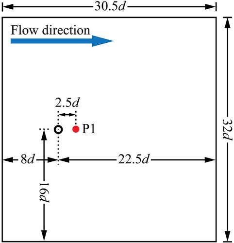
The v time series recorded at P1, shown in Fig. 2, is first extracted to analyse the characteristics of the flow state. Informed by this analysis, instantaneous flow fields, at selected time instants, are then compared in terms of streamlines and vorticity contours extracted from u and v. Finally, time-averaged velocity profiles, $\overline{u}$, are analysed along the x-directional centreline.

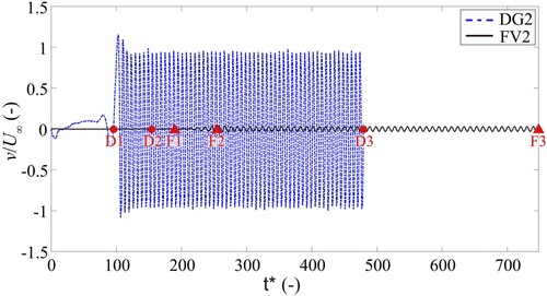
Figure 2. Flow past one cylinder: time series of the scaled transverse velocities simulated by the DG2 and FV2 solvers at R_ed = 250; D1/F1: the time when vortex shedding is triggered for DG2/FV2; D2/F2: the time when fully developed periodic quasi-steady state is established for DG2/FV2; D3/F3: the time of simulation termination for DG2/FV2.

Quasi-steady state convergence

The convergence of the DG2 and FV2 simulations to the periodic quasi-steady state is analysed. As this aspect becomes more challenging for a numerical solver with lower R_ed (Franke et al., 1990; Laroussi et al., 2014), it is first analysed for the highest R_ed = 250. Figure 2 shows the scaled v time-series recorded during the DG2 and FV2 simulations for the flow case at R_ed = 250. The captions D1–D3 and F1–F3 in Fig. 2 refer to the time when the DG2 and FV2 solvers experience different flow states, respectively. Both series exhibit periodic oscillatory patterns that reflect the presence of vortex shedding cycles, with the series of DG2 being quasi-periodic. DG2 predicts a start in the sinusoidal fluctuations, at time D1, which is around 100 t* earlier than the FV2 predictions, at time F1. The appearance of these fluctuations means that both solvers can capture the presence of vortex shedding. After nine shedding cycles, the first vortex generated advects downstream and exits at the outlet, meaning that both solvers converge to fully developed quasi-steady state with almost the same flow patterns repeating every period, at times D2 and F2, respectively. At these times, the instantaneous spatial flow patterns simulated by the DG2 and FV2 solvers are then analysed. The simulations were terminated after the next 50 vortex shedding cycles, at times D3 and F3, respectively. Rajani et al. (2009) has suggested that a period of 50 cycles is typically sufficient. Hence, time-averaged velocities were extracted from the instantaneous flow fields between the 10th and 60th cycles. This applies to both cases of flow past a single cylinder and the cylinder array.

The convergence properties of the DG2 and FV2 solvers are assessed by looking at t* required to reach quasi-steady state, the GPU runtime cost, and shedding frequency predicted. From Fig. 2, it can be seen that DG2 requires 95.5 t* (D1, Fig. 2), whereas FV2 takes 190 t* (F1, Fig. 2) to excite the vortex shedding. In this sense, DG2 is about twice as fast as FV2 to converge to a fully developed quasi-periodic steady state. Their GPU runtimes are recorded at the time when the vortex shedding was first triggered (D1 and F1, Fig. 2), when it fully developed in the quasi-steady state profile (D2 and F2, Fig. 2), and at the end of the simulation after 50 cycles (D3 and F3, Fig. 2), respectively. These runtimes for DG2 at a grid resolution of 0.25d are 3, 5 and 11 min, whereas the runtimes for FV2 at a 10-fold finer resolution of 0.025d are 84, 70 and 90 times slower, respectively. See Appendix A for a detailed analysis of GPU runtime costs comparing the DG2 and FV2 solvers.

The predicted S_t values are obtained after detecting f_s from the v time-series using fast Fourier transforms. Table 2 includes the S_t values predicted by the DG2 and FV2 solvers and the value from the reference prediction for R_ed = 250 (Rajani et al., 2009). It can be seen that the S_t values predicted by DG2 and FV2 are both lower than the reference S_t value. This is expected with inviscid SWE numerical solvers lacking kinematic and eddy viscosity (Y. Li et al., 2009), and indicates that both DG2 and FV2 solvers cannot precisely reproduce the wake evolution. However, the S_t value from the FV2 solver is much further from the reference value, suggesting that its predictions of the flow fields are more severely affected than the DG2 predictions.

Table 2. Flow past one cylinder: S_t values predicted by the FV2 and DG2 SWE solvers for flow cases at R_ed = 47, 200 and 250. These values are compared with those reported in Qu et al. (2013) and Rajani et al. (2009) from 2D RANS models whose grid resolutions around the cylinders are very fine, of 0.0054d and 0.0001d, respectively.

	St (−)
Red (−)	Reference	DG2	FV2
47	0.124 (Qu et al., 2013)	0.142	–
200	0.196 (Qu et al., 2013; Rajani et al., 2009)	0.152	–
250	0.205 (Rajani et al., 2009)	0.155	0.105

“–” indicates no data were obtained.

At R_ed = 200, no S_t value is extracted for FV2 as it did not trigger any vortex shedding (instead it predicted a constant v time series that is not shown). Refinement of the grid is expected to reduce the numerical viscosity with the FV2 solver to make it potentially able to trigger vortex shedding; but at a computational cost that cannot be justified practically. In contrast the DG2 solver, even at a 10-fold coarser grid resolution, preserves its ability to predict vortex shedding cycles as R_ed reduces. This can be confirmed by considering its predicted S_t value of 0.152 (Table 2), which, although lower than the reference S_t, is in agreement with values from the reference prediction for R_ed = 200 (Qu et al., 2013; Rajani et al., 2009). The same is observed for the flow at the lowest R_ed = 47, where excitation of vortex shedding is even more difficult for the solvers in the near-cylinder flow region where viscosity effects are higher (Balachandar et al., 1997; Braza et al., 1986). As expected, in this case, FV2 also fails to predict the formation of any vortex and DG2 predicts a S_t value of 0.142, which is slightly higher than the S_t value of 0.124 seen with the reference prediction for a similar flow at R_ed = 47 (Qu et al., 2013).

Instantaneous streamlines and vorticity contours

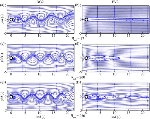
Figure 3 compares the instantaneous streamlines generated from the flow fields simulated by the DG2 and FV2 solvers after nine shedding cycles, for the flow cases at R_ed = 47, 200 and 250. At R_ed = 250, both DG2 and FV2 solvers simulate the closed vortex occurring downstream of the cylinder (Fig. 3e vs. f). Compared with the FV2 simulation, DG2 simulates the vortex closer to the cylinder, which suggests that it produces a flow pattern that is in a better agreement with the expected flow (Zdravkovich, 1997). Far downstream of the cylinder, DG2 simulates streamline fluctuations that are more pronounced than those simulated by FV2, which indicates that DG2 also performs better in capturing the details of the flow fields in the far wake. For the lower R_ed of 200 and 47 (Fig. 3c vs. d, and Fig. 3a vs. b), the better performance of DG2 is even more noticeable. DG2 captures the swirling vortex shedding from the cylinder and the associated streamline fluctuations, which were not present within the FV2 simulations. Instead, FV2 seems to simulate elongated recirculation zones without any sign of vortex formation or waviness in the simulated streamlines.

Figure 3. Flow past one cylinder: instantaneous streamlines at the start of the fully developed quasi-steady state; The left panel contains the DG2 simulated results (at time D2 in Fig. 2), while the right panel contains the FV2 simulated results (at time F2 in Fig. 2). From top to bottom, the flow cases are at R_ed = 47, 200 and 250, respectively.

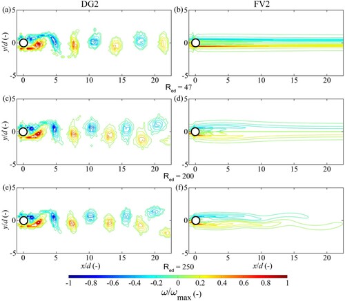
The scaled vorticity $\omega$ contours processed from the DG2 and FV2 flow fields are shown in Fig. 4. It can be seen that the DG2 solver can reproduce the evolution of the shedding vortices featured with a decay of the peak vorticity within the core of each vortex, producing classical vorticity patterns such as those reported in Ponta (2010). These vorticity patterns exhibit the S-shaped detachment from the cylinder’s surface, agreeing with the reference predictions (compare with Fig. 13 in Qu et al., 2013 and Fig. 8 in Rajani et al., 2009). This suggests that the DG2 solver has an advantage in treating the advective fluxes, as it represents the cylinders as piecewise-planar bed slope terms and reduces the amount of numerical viscosity. This makes it a better alternative to predict local flow discontinuities and thereby a more accurate prediction of vortical structure. Nonetheless, compared with the reference cases, the DG2 vorticity distributions are sparser for R_ed = 200 and 250, and exhibit a higher frequency for R_ed = 47, which is consistent with the aforementioned deviations between the S_t value predicted by DG2 and the reference values. In contrast, FV2 fails to reproduce the typical vorticity patterns for R_ed = 47, 200 and 250 (Fig. 4, right), leading to an almost symmetrical and elongated wake flow.

Figure 4. Flow past one cylinder: Instantaneous scaled vorticity contours at the start of the fully developed quasi-steady state. The left panel provides the results processed from DG2 flow fields (at time D2 in Fig. 2) and the right panel provides the results processed from FV2 flow fields (at time F2 in Fig. 2). From top to bottom, each row refers to the flow cases at R_ed = 47, 200 and 250, respectively.

Time-averaged longitudinal velocity

Figure 5 compares the scaled time-averaged longitudinal velocity $\overline{u}$ profile along the wake centreline y/d = 0 simulated by the DG2 and FV2 solvers with the reference predictions reported in Qu et al. (2013). In the figure, x = 0 is the location of the cylinder, 0 ≤ x ≤ 0.5d represents the cylinder radius shown as the light grey shading, 0.5d < x ≤ 4d covers the near-cylinder region, and the area spanning x > 4d represents the far-wake region. The recirculation length is the distance starting from the cylinder edge to the point where $\overline{u}$ changes its sign to positive. The velocity recovery rate can be analysed by looking at the gradient of the slope in the $\overline{u}$ profile. It should be noted that the profile generated for R_ed = 250 is excluded from the analysis as no reference data are found for quasi-steady flow case at this R_ed.

Figure 5. Flow past one cylinder: Profiles of the time-averaged longitudinal velocity simulated by DG2 (blue lines) and FV2 (black lines) extracted along centreline y/d = 0 relative to the reference profiles (red lines) at R_ed = 47 (solid lines) and 200 (dashed lines). The light grey shade indicates the cylinder.

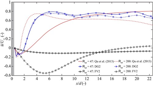
At R_ed = 200, the $\overline{u}$ profile simulated by DG2 (blue dashed line with square markers) is in a reasonable agreement with the reference $\overline{u}$ profile (red dashed line). In the near-cylinder region, the $\overline{u}$ profile simulated by DG2 is below but nearly parallel to the reference profile and lags behind it by 0.8d before reaching the same peak of 0.75. This suggests that DG2 can reproduce an almost consistent velocity recovery rate but yields an elongated recirculation length. In the far-wake region, DG2 slightly overpredicts the reference profile but maintains a similar (decreasing) trend with minor fluctuations. In contrast, the FV2 simulated $\overline{u}$ profile (black dashed line with circle markers) is negative until x > 18d, and shows a much longer recirculation length and a much slower velocity recovery rate than the reference profile. In particular, at x = 5d, FV2 reaches the lowest value of −0.55, whereas the associated reference value is around 0.7, reinforcing that FV2 tends to yield simulation results that deviate significantly from expected behaviour.

At R_ed = 47, as the viscosity effect becomes more dominant, the $\overline{u}$ profile simulated by DG2 (blue solid line with square markers) shows less agreement with the reference $\overline{u}$ profile (red solid line). In the near-cylinder region, DG2 overpredicts the reference $\overline{u}$ profile and exhibits a much steeper slope, showing that a DG2 prediction would lead to faster velocity recovery rate and shorter recirculation length. In the far-wake region, the $\overline{u}$ profile simulated by DG2 tends to become closer to the reference profile with increased distance, x > 15d. Again, FV2 (black solid line with circle markers) fails to capture the velocity recovery behind the cylinder and the negative $\overline{u}$ along the centreline indicates persistent velocity deficit downstream. This is in noticeable disagreement with the reference numerical result.

Hence, it could be inferred from the results that, when applied to simulate flow past a cylinder, the DG2 solver is a much better choice than the conventional FV2 solver, to at least produce reliable results in the far-wake region regardless of R_ed. Near the cylinder, the reliability of the DG2 simulations seems to be R_ed-dependent: with a fairly high R_ed, around 200 and higher, the DG2 simulated profiles are closer to the reference profiles than with very low R_ed, around 47. Still, given the absence of kinematic and eddy viscosity in the present DG2 solver, it is expected to yield profiles with an elongated recirculation length for transitional R_ed and with underestimated recirculation length with laminar R_ed.

The analyses of Section 3.1 suggest that a DG2 solver’s run at a resolution of 0.25d is much faster to trigger vortex shedding than an FV2 solver’s run at a 10-fold finer resolution of 0.025d, making it 90 times faster to complete a converged simulation. Therefore, the DG2 solver is a more accurate and efficient alternative to simulate flow within cylinder arrays to at least capture the flow characteristics in the far-wake region. This will be investigated next with respect to a new laboratory-scale application.

3.2 Flow within an array of cylinders

The DG2 solver is further explored through the simulation of experimental flow fields within randomly distributed cylinders of diameter d = 4 mm in a 3750d × 75d flume. The experiment was conducted at the University of Warwick, and involved SPIV measurements of instantaneous u and v data (Corredor-Garcia et al., 2020; Sonnenwald, Stovin et al., 2019). Within the flume, a random distribution of cylinders was generated for a 625d × 75d baseplate, and duplicates of this baseplate were used to cover a total length of 1875d (Fig. 6a). SPIV data (Corredor-Garcia et al., 2020) was collected for an area 137.5d × 75d, located 1332.5d from the start of the cylinder section (Fig. 6b), i.e. in a downstream section where the flow was believed to be fully developed. The computational domain covered the full 1875d channel length, again to ensure that the flow field was fully developed. Four cases with different R_ed are reported (Corredor-Garcia et al., 2021), but for consistency with Section 3.1, only the flows with the lowest and highest R_ed of 53 and 220, representing the laminar and transitional flow regimes, are investigated here. Table 3 shows the hydraulic and experimental parameters used to run the DG2 simulations for each of the selected R_ed. It should be noted that the projection bias from the SPIV measurement has not been corrected, and this therefore shifts the measured cylinder positions. The cylinders project above the surface of the flow, which leads to missing hydrodynamic information (data shadows) where visualization of the flow surface is blocked by the projected cylinders. Finally, it should also be noted that, whereas the laboratory cylinders were truly cylindrical, the numerical cylinders are approximated by rectilinear shapes on the 1 mm square computational grid.

Figure 6. Flow within an array of cylinders: (a) schematic plan view of the randomly distributed cylinders in the flume; (b) cylinder spatial distribution in the SPIV measurement section (Corredor-Garcia et al., 2020; Sonnenwald, Stovin et al., 2019).

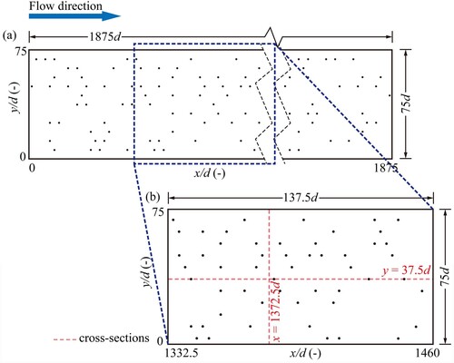
Table 3. Flow within an array of cylinders: the hydraulic and experimental parameters for flow cases at R_ed = 53 and 220.

Red (–)	U∞ (m s^−1)	h (m)	qx (m^2 s^−1)	S0 (m m^−1)	nM (m^1/6)
53	0.0147	0.15	0.002205	0.0	0.045
220	0.06		0.009	4.6 × 10^−4

The DG2 simulations are run on a grid with the same resolution identified in Section 3.1 (i.e. 1 mm), which also matches the 1 mm pixel resolution of the SPIV datasets. The DG2 simulated instantaneous u and v components of velocity are recorded at the same time interval as the SPIV measuring frequency of 25 frames per second to allow for consistent comparisons. The shedding frequencies are first analysed to study quasi-steady state convergence, and further investigations are done using time-averaged 2D velocity maps and 1D profiles along the longitudinal and transverse cross sections y = 1372.5d and x = 50d, respectively. The average deviation errors between the simulated and SPIV velocity data are quantified using the L¹-norm error that is expressed as: (2) ${\mathsf{L}}^{\mathsf{1}}\text{ - norm error = }\frac{\text{1}}{N}\left(\sum _{k\text{ = 1}}^N|z_k^{Num}-z_k^{Ref}|\right)$(2) where N denotes the number of grid elements, and $z_k^{Num}$ and $z_k^{Ref}$ are the respective numerically simulated and reference $\overline{u}$ or $\overline{v}$ values. To quantify the extent of directional alignment between the simulated and reference flow fields, the Relevance Index (R_I) is used, defined as: (3) ${\mathsf{R}}_{\mathsf{I}}=\frac{\text{1}}{N}\left(\sum _{k=1}^N\frac{〈V_k^{Num},V_k^{Ref}〉}{\Vert V_k^{Num}\Vert \Vert V_k^{Ref}\Vert }\right)$(3) where V is the time-averaged velocity vector consisting of components $\overline{u}$ and $\overline{v}$, <> denotes the inner product operator, and || || indicates the magnitude of $V=\sqrt{{\overline{u}}^{\text{2}}\text{ + }{\overline{v}}^{\text{2}}}$. The R_I takes values between −1 and 1, with 1 indicating a perfect alignment of the simulated and reference velocity vectors.

Quasi-steady state convergence

For each flow case, the simulation is set to terminate after 50 cycles when a fully developed quasi-periodic steady state is reached, informed by the analysis of Section 3.1. Steady state convergence is analysed in terms of vortex shedding frequency f_s and Strouhal number S_t. Since the flow is influenced by the background turbulence imposed by the adjacent cylinders (Nepf, 1999; Ricardo, Sanches et al., 2016), f_s values sampled behind all the cylinders should have a range of variations. Table 4 also includes the mean and standard deviation values for simulated and measured f_s and S_t, which have been derived from the time histories of v for all the cylinders located within the portion of SPIV data measurements, at a distance of 2.5d behind each cylinder’s centre. For both flow cases at R_ed = 53 and 220, the mean values for f_s and S_t simulated by the DG2 solver are lower than the estimates from the SPIV data. This discrepancy may be due to the overpredicted velocities near the sidewalls (as shown later in Fig. 7), which may exert an influence on the wake flow evolution and thereby distort the shedding frequency. Still, for both cases, the DG2 predicted ranges for standard deviation of f_s and S_t are close to the ranges estimated from the SPIV data, showing a satisfactory level of agreement. The associated time-averaged velocities extracted over the 50 cycles are then analysed.

Figure 7. Flow within an array of cylinders: contours of the scaled time-averaged longitudinal velocity and the L¹-norm errors. The upper panel contains the results for the flow case at R_ed = 53: (a) SPIV measurement and (b) DG2 simulation, while the lower panel contains those for the flow case at R_ed = 220: (c) SPIV measurement and (d) DG2 simulation.

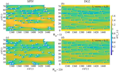
Table 4. Flow within an array of cylinders: DG2 simulated and SPIV measured shedding frequencies and S_t ranges for the cylinder array within the SPIV measurement section for each flow condition after 50 shedding cycles.

	fs (s^−1)		St (−)
Red (−)	SPIV	DG2	SPIV	DG2
53	0.56 ± 0.2	0.4 ± 0.21	0.15 ± 0.054	0.11 ± 0.057
220	2.9 ± 0.8	1.6 ± 0.85	0.2 ± 0.055	0.11 ± 0.057

Time-averaged scaled flow fields

Figure 7 compares the scaled $\overline{u}$ contour maps obtained from the DG2 solver’s simulations to the measured ones at R_ed = 53 and 220, showing generally good agreement. This is confirmed by the small magnitude of the L¹-norm errors (≤0.2). Note that these errors may be higher than expected, being affected by the aforementioned projection bias in the SPIV data. At R_ed = 53 (Fig. 7b vs. a), DG2 simulates elongated wake flow areas behind all the cylinders as compared with the measured data. The observed over-expansion of the wake flow patterns is expected to occur due to the mismatch between numerical viscosity and true kinematic and eddy viscosity. At the higher R_ed = 220 (Fig. 7d vs. c), the simulated $\overline{u}$ map better matches the measured $\overline{u}$ map, as the L¹-norm error is smaller. This indicates a better performance for the DG2 solver at R_ed = 220 where there is more dominance from the advective fluxes over the viscosity effects. This also implies that the DG2 solver introduces an amount of numerical viscosity for the flow at the higher R_ed that helps imitate the effects of the true kinematic and eddy viscosity. The most noticeable differences between the measured and simulated flow fields are in the right hand one third of the channel (0 < y/d < 30) where a high velocity preferential flow path forms between widely-spaced cylinders; this is far less evident in the simulation compared with the measured data. Also, for both flow cases, the simulated $\overline{u}$ near the sidewalls are overpredicted, and this may be caused by the lack of an explicit wall treatment function within the DG2 solver (Ginting, 2019).

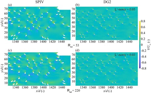
In Fig. 8, the scaled $\overline{v}$ contour maps acquired from the DG2 simulations are compared with the measured $\overline{v}$ maps at R_ed = 53 and 220. Generally, the simulated $\overline{v}$ maps are in close agreement with measured maps and the L¹-norm errors are not greater than 0.05. The DG2 solver is seen to reproduce the alternating and symmetrical patterns along each cylinder’s wake centreline, which are observed in the measured $\overline{v}$ maps. At R_ed = 53 (Fig. 8b vs. a), the measured $\overline{v}$ patterns along the cylinders are bigger in magnitude than the simulated patterns. This underestimation of transverse velocities implies that the simulation tends to underestimate the extent to which the streamlines curve around the cylinders. Reduced streamline curvature is also evident in the velocity vector maps (as shown later in Fig. 11). This may arise as a result of the rectilinear representation of the cylinder geometry, and the mismatch between numerical viscosity and true kinematic and eddy viscosity. At R_ed = 220, the simulated patterns agree better with the measured patterns for $\overline{v}$ (Fig. 8d vs. c), which is in line with the better agreement observed between the simulated and measured $\overline{u}$ at R_ed = 220 (recall Fig. 7).

Figure 8. Flow within an array of cylinders: contours of the scaled time-averaged transverse velocity and the L¹-norm errors. The upper panel contains the results for the flow case at R_ed = 53: (a) SPIV measurement and (b) DG2 simulation, while the lower panel contains those for the flow case at R_ed = 220: (c) SPIV measurement and (d) DG2 simulation.

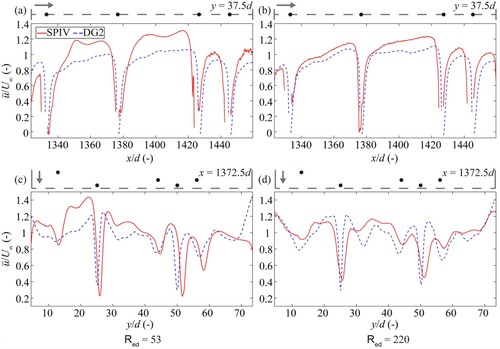
To closely analyse the simulated wake flow features, Fig. 9 compares the simulated and measured $\overline{u}$ profiles along y = 37.5d and x = 1372.5d, for R_ed = 53 (left) and 220 (right). Along y = 37.5d (Fig. 9a and b), the $\overline{u}$ profiles are only analysed up to the second cylinder (the predictions around the last two cylinders may be subject to position shift from the projection bias). At R_ed = 53, in the near-cylinder regions, the simulated profile (blue dashed line) is above the measured one (red solid line) with a steeper slope, showing that DG2 overpredicts the measured $\overline{u}$ magnitude as observed in the findings of Section 3.1. In the far-wake regions, the simulated profile is below but almost parallel to the measured profile, confirming that DG2 produces a similar velocity recovery rate to the measured one but underestimates the $\overline{u}$ magnitudes. Such underestimation of the $\overline{u}$ magnitudes also reflects the difference between the simulated and measured $\overline{u}$ contours in the far-wake regions, as discussed previously for Fig. 7a and b. At R_ed = 220, the simulated $\overline{u}$ profile achieves a closer agreement with the measured profile than that at R_ed = 53, which again reinforces that the DG2 solver predicts closer results at higher R_ed. Along x = 1372.5d, at R_ed = 53 (Fig. 9c), the simulated $\overline{u}$ profile agrees well with the measured one, albeit with slight deviations due to the projection bias. At R_ed = 220 (Fig. 9d), the DG2 solver produces a generally good agreement with the measured profile but yields sharper peaks near the two cylinders spanning 20d < y < 30d and 45d < y < 55d.

Figure 9. Flow within an array of cylinders: time-averaged longitudinal velocity profiles measured by SPIV (red solid lines) and simulated by DG2 (blue dashed lines), at R_ed = 53 (left) and 220 (right). (a) and (b) show the profiles along y = 37.5d. (c) and (d) show the profiles along x = 1372.5d. The upper part of each sub-plot shows the positions of cylinders (black dots) and the flow direction (grey arrows).

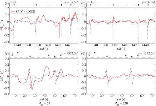
From Fig. 10, a similar analysis can be conducted for the simulated and measured $\overline{v}$ profiles. Along y = 37.5d, at R_ed = 53 (Fig. 10a), the simulated profile (blue dashed line) deviates from the measured profile (red solid line), which is expected, as the overall variation in measured $\overline{v}$ is more pronounced compared with the simulation (recall Fig. 8a vs. b). However, at R_ed = 220 (Fig. 10b), the simulated $\overline{v}$ profile is very close to the measured profile. Along x = 1372.5d, at R_ed = 53 (Fig. 10c), the DG2 solver produces smoother variations in the simulated $\overline{v}$ compared with the measured $\overline{v}$ that have lower magnitudes. At R_ed = 220 (Fig. 10d), the simulated profile resembles the measured profile but DG2 yields sharper $\overline{v}$ peaks within zones 20d < y < 30d and 45d < y < 55d. Such overestimation is expected due to the rectilinear representation of the cylinders, as discussed previously for Fig. 8.

Figure 10. Flow within an array of cylinders: time-averaged transverse velocity profiles measured by SPIV (red solid lines) and simulated by DG2 (blue dashed lines), at R_ed = 53 (left) and 220 (right). (a) and (b) show the profiles along y = 37.5d. (c) and (d) show the profiles along x = 1372.5d. The upper part of each sub-plot shows the positions of cylinders (black dots) and the flow direction (grey arrows).

Figure 11 displays the R_I fields calculated from the simulated and measured velocity vectors for flow cases at R_ed = 53 (top panel) and 220 (bottom panel), to further assess the agreement in directionalities of flow fields. Figure 11a and c show the R_I fields within the whole measurement section. Figure 11b and d illustrate the zoomed-in view of the simulated and measured time-averaged velocity vectors superimposed onto the R_I fields, which are around the cylinder located at (1370.3d, 25d). This cylinder was selected due to the overlap between the position of the simulated cylinder and the measured one. Within data shadows, the green circle indicates the actual cylinder position, the area with black outline represents the simulated cylinder, and the light grey shading shows the blocked hydrodynamic information around the measured cylinder.

Figure 11. Flow within an array of cylinders: Relevance Index fields (left panel) and zoomed-in view of spatial velocity vectors of DG2 (blue arrows) and SPIV (red arrows) superimposed onto Relevance Index fields and around one cylinder x, y = 1370.3d, 25d (right panel); The upper panel (a and b) is for the flow case at R_ed = 53, whereas the lower panel (c and d) is for the flow case at R_ed = 220. The Relevance Index coefficients are provided in each panel.

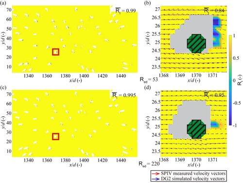
At R_ed = 53, Fig. 11a shows a fairly strong alignment between the simulated and measured flow directions in the majority of the R_I field. This can be confirmed by the whole mean R_I value which is close to 1. However, misalignment of the flow direction can be seen in the areas around the cylinders, owing to the difference between the simulated and measured cylinder positions and data shadows. Figure 11b clearly identifies this relatively poor alignment, and the mean R_I value in this zoomed-in portion, of 0.84 is lower than the whole mean R_I value of 0.99. There are small included angles between some of the simulated and measured velocity vectors. The greater curvature visible in the measured vectors is consistent with the fact that the magnitude of measured $\overline{v}$ around the cylinder is higher than the simulated one (recall Fig. 8a and b). At R_ed = 220 (Fig. 11c), the simulated flow direction almost perfectly matches the measured one as the whole mean R_I value is very close to 1. Figure 11d shows that the DG2 solver can closely reproduce the measured velocity vectors around the cylinder. The mean R_I value in the zoomed-in portion of 0.95 indicates a better directional alignment at higher R_ed.

Overall, the analysis in Section 3.2 confirms that the DG2 solver can reproduce the complex wake evolution patterns and closely reproduce the flow directions around cylinders, and the reliability of its predictions would be enhanced with the increase in R_ed. This suggests that the DG2 solver can be a practical modelling tool for environmental hydraulic applications involving a quasi-steady, slow flow past large-scale cylinder arrays in the higher R_ed regimes.

4 Conclusions

Inviscid numerical solvers of the two-dimensional (2D) depth-averaged SWE integrate the advective fluxes and bed slope terms and use Manning’s formula as an implicit model of the vertical turbulence structure. Although these solvers exclude the viscous and turbulent eddy viscosity terms, they introduce an amount of numerical viscosity that may imitate many of the mechanisms of viscous turbulent models for low R_ed. When simulating laminar to transitional wakes past cylinder(s) in slow quasi-steady flows (R_ed ≤ 250), an FV2 SWE solver fails to detect the wake formation at practically affordable grid resolution. It is affected by fast growth of numerical error dissipation that manifests as large numerical viscosity. The extra numerical complexity in a DG2 SWE solver provides a more accurate treatment of the advective fluxes and bed slope terms, generally resulting in better predictions at coarser grid resolutions and much lower numerical viscosity.

The advantage of the DG2 solver over the FV2 solver was first diagnostically evaluated in simulating wake evolution for classical flows past a single cylinder. The comparative analysis included convergence speed to complete 50 vortex shedding cycles, ability to excite and capture periods of vortex shedding, and to capture vortical structures and longitudinal velocity profiles. The analysis confirms that the DG2 solver is more suited to efficiently model the wake formation, despite the limitation of solving the inviscid SWE. Therefore, its reliability to predict the wake formation improves with a R_ed > 200 compared to a R_ed around 50 where viscosity effects are more significant. This capability for the DG2 solver was then verified by applying it to reproduce laboratory-scale flows past an array of randomly distributed cylinders with validation against measured velocity fields. The laboratory-scale tests reinforce that the DG2 SWE solver is a useful tool to efficiently simulate sufficiently accurate wake formations that would resemble the measurements and those produced by more complex models. Being far less dissipative than the FV2 solver, the findings suggest that the DG2 solver is a promising alternative to also improve the predictive capability of depth-averaged RANS models using the SWE with the equations integrating the viscous and/or the turbulent fluxes.

Acknowledgements

We would like to thank Alexandre Delalande for conducting the experiment at the University of Warwick and providing the experimental data and parameters. We are also grateful to Jesus Leonardo Corredor-Garcia (University of Sheffield) for providing the post-processed SPIV data and his valuable expertise. We also would like to thank two anonymous reviewers for their constructive and thorough comments and suggestions. For the purpose of open access, the authors have applied a Creative Commons Attribution (CC BY) licence to any Author Accepted Manuscript version arising. Numerical simulation data, set-up files and the code to run the solvers are openly available on: https://zenodo.org/record/8146884 (last accessed July 14, 2023).

Disclosure statement

No potential conflict of interest was reported by the author(s).

Additional information

Funding

This work was supported by the UK Engineering and Physical Sciences Research Council (EPSRC) grant EP/R007349/1.

Appendix A.

Grid resolution selection

This section is aimed to justify the grid resolution selected for running the DG2 and FV2 solvers. For the scope of this study, the aim was to choose a resolution that is appropriate for a solver to trigger periodical shedding of vortices, while keeping the simulation within the GPU memory capacity and within a runtime of less than a day in order to support the needs for larger scale simulations, including the case study in Section 3.2. This choice was done diagnostically by applying both solvers to run the flow past a single cylinder of diameter d = 4 mm for R_ed = 250 (Section 3.1). The simulations were investigated on grids starting with a resolution of 0.25d, equivalent to 1 mm, and the finest resolution possible was 0.025d, equivalent to 0.1 mm. The capability of a solver to capture periodical vortex shedding was evaluated based on the predicted S_t values as compared to values of 0.205 from the reference prediction (Rajani et al., 2009). Also, the runtime efficiency of each solver at different grid resolutions was measured by considering the overall GPU runtime cost needed to complete 50 shedding cycles and the relative runtime cost per grid element. The latter was obtained by first dividing the overall GPU runtime cost by the number of elements and then scaling it with respect to the runtime cost per element of a baseline simulation. The baseline simulation was taken to be the DG2 solver run at the coarsest resolution that could trigger the vortex shedding (i.e. at the grid resolution of 0.25d). Table A.1 lists the predicted S_t values, GPU runtime costs and the relative runtime costs per element for the DG2 and FV2 solvers at different grid resolutions.

Table A1. Flow past one cylinder at R_ed = 250: S_t values predicted by the DG2 and FV2 solvers at grid resolutions between 0.25d and 0.025d, and the associated number of elements, overall GPU runtime costs as well as relative runtime cost per element.

		St (–)		Overall GPU runtime costs		Relative runtime costs per element
Resolution	No. of elements	DG2	FV2	DG2	FV2	DG2	FV2
0.25d (1 mm)	15,616	0.155	—	11 min	—	1×	—
0.125d (0.5 mm)	62,464	0.19	—	2 h	—	2.7×	—
0.0625d (0.25 mm)	249,856	0.21	—	5 h	—	1.7×	—
0.025d (0.1 mm)	1.56 million	—	0.105	—	16.5 h	—	0.9×

Reference S_t is 0.205 (Rajani et al., 2009).

“—” indicates no data were obtained.

The FV2 solvers fail to predict any S_t values except using a grid resolution of 0.025d. Relative to the baseline simulation, the FV2 solver at this grid resolution has a slightly lower relative runtime cost per element (0.9 times) but requires 90 times higher overall GPU runtime cost, taking about 16.5 h to complete the simulation. Moreover, the predicted S_t value of 0.105 is lower than that predicted by the baseline of 0.155, showing less accuracy. Note that better accuracy could not be achieved since a finer grid resolution could not be afforded for this simulation. In contrast, the DG2 solver is able to predict S_t values regardless of the grid resolutions used, except for the grid resolution of 0.025d which could not be performed due to insufficient GPU memory. Also, finer grid resolutions lead to predictions that approach the reference S_t value of 0.205. However, compared to the baseline simulation, the grid resolutions of 0.125d and 0.0625d lead to prohibitive GPU runtime costs (2 h and 5 h, respectively) and higher relative runtime costs per element (2.7 and 1.7 times, respectively). These in turn result in simulation runtimes longer than one day and exceed GPU memory limits, for the laboratory-scale case study in Section 3.2. Therefore, the grid resolution used in the baseline, 0.25d, is found to be adequate for meeting the needs of the simulations for this study.

Notation

d	=	cylinder diameter (m)
fs	=	shedding frequency (s−1)
F	=	flux vector in x-direction (–)
g	=	gravity acceleration (m s−2)
G	=	flux vector in y-direction (–)
h	=	water depth (m)
L1	=	scaled L1-norm error (–)
nM	=	Manning’s resistance parameter (m1/6)
N	=	number of gird elements (–)
qx	=	x-directional flow discharge per unit width (m2 s−1)
qy	=	y-directional flow discharge per unit width (m2 s−1)
Qc	=	computational grid element (–)
Red	=	cylinder Reynolds number (–)
RI	=	Relevance Index (–)
Sb	=	topography source term vector (–)
Sf	=	friction source term vector (–)
St	=	Strouhal number (–)
t	=	time (s)
t*	=	dimensionless time (–)
u	=	longitudinal velocity (m s−1)
$\overline{u}$	=	time-averaged longitudinal velocity (m s−1)
U	=	vector of flow variables (–)
U∞	=	steady inflow velocity (m s−1)
v	=	transverse velocity (m s−1)
$\overline{v}$	=	time-averaged transverse velocity (m s−1)
x	=	longitudinal coordinate (m)
xc	=	centre of grid in x-direction (–)
y	=	transverse coordinate (m)
yc	=	centre of grid in y-direction (–)
z	=	topography (m)
z	=	vector of topography coefficients (–)
Δt	=	time step (s)
Δx	=	length of a grid Qc in x-direction (m)
Δy	=	length of a grid Qc in y-direction (m)
υ	=	kinematic viscosity (m2 s−1)
$\omega$	=	vorticity (s−1)

Superscripts

0	=	average coefficient (–)
1x	=	x-directional slope coefficient (–)
1y	=	y-directional slope coefficient (–)

Subscripts

c	=	computational grid (–)
h	=	approximate solution (–)
nei	=	index of the direct neighbour grid (–)
W, E, S, N	=	western, eastern, southern, northern sides (–)

References

- Ayog, J. L., Kesserwani, G., Shaw, J., Sharifian, M. K., & Bau, D. (2021). Second-order discontinuous Galerkin flood model: Comparison with industry-standard finite volume models. Journal of Hydrology, 594(September 2020), 125924. https://doi.org/10.1016/j.jhydrol.2020.125924
- Ayyappan, T., & Vengadesan, S. (2008). Three-dimensional simulation of flow past a circular cylinder by nonlinear turbulence model. Numerical Heat Transfer, Part A: Applications, 54(2), 221–234. https://doi.org/10.1080/10407780802084694
- Balachandar, S., Mittal, R., & Najjar, F. M. (1997). Properties of the mean recirculation region in the wakes of two-dimensional bluff bodies. Journal of Fluid Mechanics, 351, 167–199. https://doi.org/10.1017/S0022112097007179
- Bazin, P.-H. (2013). Flows during floods in urban areas: influence of the detailed topography and exchanges with the sewer system. Université Claude Bernard – Lyon I. https://tel.archives-ouvertes.fr/tel-01159518/file/TH2013BazinPierreHenri.pdf.
- Behr, M., Liou, J., Shih, R., & Tezduyar, T. E. (1991). Vorticity-streamfunction formulation of unsteady incompressible flow past a cylinder: Sensitivity of the computed flow field to the location of the outflow boundary. International Journal for Numerical Methods in Fluids, 12(4), 323–342. https://doi.org/10.1002/fld.1650120403
- Bonetti, S., Manoli, G., Manes, C., Porporato, A., & Katul, G. G. (2017). Manning’s formula and Strickler’s scaling explained by a co-spectral budget model. Journal of Fluid Mechanics, 812, 1189–1212. https://doi.org/10.1017/jfm.2016.863
- Braza, M., Chassaing, P., & Ha Minh, H. (1986). Numerical study and physical analysis of the pressure and velocity fields in the near wake of a circular cylinder. Journal of Fluid Mechanics, 165(-1), 79–130. https://doi.org/10.1017/S0022112086003014
- Chen, L., Tu, J. Y., & Yeoh, G. H. (2003). Numerical simulation of turbulent wake flows behind two side-by-side cylinders. Journal of Fluids and Structures, 18(3–4), 387–403. https://doi.org/10.1016/j.jfluidstructs.2003.08.005
- Corredor Garcia, J., Delalande, A., Stovin, V., & Guymer, I. (2021). Surface Velocity Fields from Experiments in Flow Through Emergent Vegetation (Version 1) [Data Set]. The University of Sheffield. https://doi.org/10.15131/shef.data.16550388
- Corredor-Garcia, J. L., Delalande, A., Stovin, V., & Guymer, I. (2020). On the Use of Surface PIV for the Characterization of Wake Area in Flows Through Emergent Vegetation. Recent Trends in Environmental Hydraulics, 43–52. https://doi.org/10.1007/978-3-030-37105-0_4
- Darby, S. E. (1999). Effect of Riparian Vegetation on Flow Resistance and Flood Potential. Journal of Hydraulic Engineering, 125(5), 443–454. https://doi.org/10.1061/(ASCE)0733-9429(1999)125:5(443)
- Etminan, V., Lowe, R., & Ghisalberti, M. (2017). A new model for predicting the drag exerted by vegetation canopies. Water Resources Research, 53(4), 3179–3196. https://doi.org/10.1111/j.1752-1688.1969.tb04897.x
- Franke, R., Rodi, W., & Schönung, B. (1990). Numerical calculation of laminar vortex-shedding flow past cylinders. Journal of Wind Engineering and Industrial Aerodynamics, 35, 237–257. https://doi.org/10.1016/0167-6105(90)90219-3
- Gao, Y., Qu, X., Zhao, M., & Wang, L. (2019). Three-dimensional numerical simulation on flow past three circular cylinders in an equilateral-triangular arrangement. Ocean Engineering, 189, 106375. https://doi.org/10.1016/j.oceaneng.2019.106375
- Ginting, B. M. (2019). Central-upwind scheme for 2D turbulent shallow flows using high-resolution meshes with scalable wall functions. Computers & Fluids, 179, 394–421. https://doi.org/10.1016/j.compfluid.2018.11.014
- Ginting, B. M., & Ginting, H. (2019). Hybrid Artificial Viscosity–Central-Upwind Scheme for Recirculating Turbulent Shallow Water Flows. Journal of Hydraulic Engineering, 145(12), 1–17. https://doi.org/10.1061/(asce)hy.1943-7900.0001639
- Gioia, G., & Bombardelli, F. A. (2001). Scaling and Similarity in Rough Channel Flows. Physical Review Letters, 88(1), 4. https://doi.org/10.1103/PhysRevLett.88.014501
- Golzar, M. (2018). CFD modelling of dispersion within randomly distributed cylinder arrays. The University of Sheffield. https://etheses.whiterose.ac.uk/22887/1/MahshidGolzar PhD Thesis.pdf
- Hamidifar, H., Omid, M. H., & Keshavarzi, A. (2015). Longitudinal dispersion in waterways with vegetated floodplain. Ecological Engineering, 84, 398–407. https://doi.org/10.1016/j.ecoleng.2015.09.048
- Hinterberger, C., Fröhlich, J., & Rodi, W. (2007). Three-Dimensional and Depth-Averaged Large-Eddy Simulations of Some Shallow Water Flows. Journal of Hydraulic Engineering, 133(8), 857–872. https://doi.org/10.1061/_ASCE0733-9429_2007133:8_857
- Jiang, H., & Cheng, L. (2017). Strouhal-Reynolds number relationship for flow past a circular cylinder. Journal of Fluid Mechanics, 832, 170–188. https://doi.org/10.1017/jfm.2017.685
- Jiang, H., & Cheng, L. (2021). Large-eddy simulation of flow past a circular cylinder for Reynolds numbers 400 to 3900. Physics of Fluids, 33(3), 034119. https://doi.org/10.1063/5.0041168
- Jiang, H., Cheng, L., Draper, S., An, H., & Tong, F. (2016). Three-dimensional direct numerical simulation of wake transitions of a circular cylinder. Journal of Fluid Mechanics, 801, 353–391. https://doi.org/10.1017/jfm.2016.446
- Kesserwani, G. (2013). Topography discretization techniques for Godunov-type shallow water numerical models: A comparative study. Journal of Hydraulic Research, 51(4), 351–367. https://doi.org/10.1080/00221686.2013.796574
- Kesserwani, G., Ayog, J. L., & Bau, D. (2018). Discontinuous Galerkin formulation for 2D hydrodynamic modelling: Trade-offs between theoretical complexity and practical convenience. Computer Methods in Applied Mechanics and Engineering, 342, 710–741. https://doi.org/10.1016/j.cma.2018.08.003
- Kesserwani, G., Ayog, J. L., Sharifian, M. K., & Baú, D. (2023). Shallow-Flow Velocity Predictions Using Discontinuous Galerkin Solutions. Journal of Hydraulic Engineering, 149(5). https://doi.org/10.1061/jhend8.hyeng-13244
- Kesserwani, G., Ghostine, R., Vazquez, J., Ghenaim, A., & Mosé, R. (2008). Riemann Solvers with Runge–Kutta Discontinuous Galerkin Schemes for the 1D Shallow Water Equations. Journal of Hydraulic Engineering, 134(2), 243–255. https://doi.org/10.1061/(ASCE)0733-9429(2008)134:2(243)
- Kesserwani, G., & Wang, Y. (2014). Discontinuous Galerkin flood model formulation: Luxury or necessity? Water Resources Research, 50(8), 6522–6541. https://doi.org/10.1002/2013WR014906
- Kim, H. S., Kimura, I., & Park, M. (2018). Numerical Simulation of Flow and Suspended Sediment Deposition Within and Around a Circular Patch of Vegetation on a Rigid Bed. Water Resources Research, 54(10), 7231–7251. https://doi.org/10.1029/2017WR021087
- Kim, H. S., Nabi, M., Kimura, I., & Shimizu, Y. (2015). Computational modeling of flow and morphodynamics through rigid-emergent vegetation. Advances in Water Resources, 84, 64–86. https://doi.org/10.1016/j.advwatres.2015.07.020
- King, A. (2006). Field measurements of bulk flow and transport through a small coastal embayment having variable distributions of aquatic vegetation. Cornell University. https://ecommons.cornell.edu/handle/1813/3438.
- Kitagawa, T., & Ohta, H. (2008). Numerical investigation on flow around circular cylinders in tandem arrangement at a subcritical Reynolds number. Journal of Fluids and Structures, 24(5), 680–699. https://doi.org/10.1016/j.jfluidstructs.2007.10.010
- Laroussi, M., Djebbi, M., & Moussa, M. (2014). Triggering vortex shedding for flow past circular cylinder by acting on initial conditions: A numerical study. Computers & Fluids, 101, 194–207. https://doi.org/10.1016/j.compfluid.2014.05.034
- Li, L., Yan, Z., & Liu, Z. (2012). Numerical model for shallow wake behind cylinder. Applied Mechanics and Materials, 212–213, 1205–1212. https://doi.org/10.4028/www.scientific.net/AMM.212-213.1205
- Li, W., Ren, J., Hongde, J., Luan, Y., & Ligrani, P. (2016). Assessment of six turbulence models for modeling and predicting narrow passage flows, part 2: Pin fin arrays. Numerical Heat Transfer, Part A: Applications, 69(5), 445–463. https://doi.org/10.1080/10407782.2015.1081024
- Li, Y., Zhang, R., Shock, R., & Chen, H. (2009). Prediction of vortex shedding from a circular cylinder using a volumetric Lattice-Boltzmann boundary approach. The European Physical Journal Special Topics, 171(1), 91–97. https://doi.org/10.1140/epjst/e2009-01015-9
- Macías, J., Castro, M. J., & Escalante, C. (2020). Performance assessment of the Tsunami-HySEA model for NTHMP tsunami currents benchmarking. Laboratory data. Coastal Engineering, 158(July 2018), 103667. https://doi.org/10.1016/j.coastaleng.2020.103667
- Marjoribanks, T. I., Hardy, R. J., Lane, S. N., & Tancock, M. J. (2017). Patch-scale representation of vegetation within hydraulic models. Earth Surface Processes and Landforms, 42(5), 699–710. https://doi.org/10.1002/esp.4015
- Mittal, S. (2005). Excitation of shear layer instability in flow past a cylinder at low Reynolds number. International Journal for Numerical Methods in Fluids, 49(10), 1147–1167. https://doi.org/10.1002/fld.1043
- Nepf, H. M. (1999). Drag, turbulence, and diffusion in flow through emergent vegetation. Water Resources Research, 35(2), 479–489. https://doi.org/10.1029/1998WR900069
- Nishino, T., Roberts, G. T., & Zhang, X. (2008). Unsteady RANS and detached-eddy simulations of flow around a circular cylinder in ground effect. Journal of Fluids and Structures, 24(1), 18–33. https://doi.org/10.1016/j.jfluidstructs.2007.06.002
- O’Hare, M. T. (2015). Aquatic vegetation - A primer for hydrodynamic specialists. Journal of Hydraulic Research, 53(6), 687–698. https://doi.org/10.1080/00221686.2015.1090493
- Ponta, F. L. (2010). Vortex decay in the Kármán eddy street. Physics of Fluids, 22(9), 1–11. https://doi.org/10.1063/1.3481383
- Qu, L., Norberg, C., Davidson, L., Peng, S. H., & Wang, F. (2013). Quantitative numerical analysis of flow past a circular cylinder at Reynolds Number between 50 and 200. Journal of Fluids and Structures, 39, 347–370. https://doi.org/10.1016/j.jfluidstructs.2013.02.007
- Rajani, B. N., Kandasamy, A., & Majumdar, S. (2009). Numerical simulation of laminar flow past a circular cylinder. Applied Mathematical Modelling, 33(3), 1228–1247. https://doi.org/10.1016/j.apm.2008.01.017
- Rastogi, A. K., & Rodi, W. (1978). Predictions of Heat and Mass Transfer in Open Channels. Journal of the Hydraulics Division, 104(3), 397–420. https://doi.org/10.1061/JYCEAJ.0004962
- Ricardo, A. M., Franca, M. J., & Ferreira, R. M. L. (2016). Turbulent Flows within Random Arrays of Rigid and Emergent Cylinders with Varying Distribution. Journal of Hydraulic Engineering, 142(9), 04016022. https://doi.org/10.1061/(asce)hy.1943-7900.0001151
- Ricardo, A. M., Sanches, P. M., & Ferreira, R. M. L. (2016). Vortex shedding and vorticity fluxes in the wake of cylinders within a random array. Journal of Turbulence, 17(11), 999–1014. https://doi.org/10.1080/14685248.2016.1212166
- Rizzi, A. (1982). Mesh Influence on Vortex Shedding in Inviscid Flow Computations. In Recent Contributions to Fluid Mechanics (pp. 213–221). Springer Berlin Heidelberg.
- Schär, C., & Smith, R. B. (1993). Shallow-Water Flow past Isolated Topography. Part I: Vorticity Production and Wake Formation. Journal of the Atmospheric Sciences, 50(10), 1373–1400. https://doi.org/10.1175/1520-0469(1993)050<1373:SWFPIT>2.0.CO;2
- Seo, I. W., & Song, C. G. (2012). Numerical simulation of laminar flow past a circular cylinder with slip conditions. International Journal for Numerical Methods in Fluids, 68(12), 1538–1560. https://doi.org/10.1002/fld.2542
- Shaw, J., Kesserwani, G., Neal, J., Bates, P., & Sharifian, M. K. (2021). LISFLOOD-FP 8.0: The new discontinuous Galerkin shallow-water solver for multi-core CPUs and GPUs. Geoscientific Model Development, 14(6), 3577–3602. https://doi.org/10.5194/gmd-14-3577-2021
- Sonnenwald, F., Guymer, I., & Stovin, V. (2019). A CFD-Based Mixing Model for Vegetated Flows. Water Resources Research, 55(3), 2322–2347. https://doi.org/10.1029/2018WR023628
- Sonnenwald, F., Hart, J. R., West, P., Stovin, V. R., & Guymer, I. (2017). Transverse and longitudinal mixing in real emergent vegetation at low velocities. Water Resources Research, 53(1), 961–978. https://doi.org/10.1002/2016WR019937
- Sonnenwald, F., Stovin, V., & Guymer, I. (2019). A stem spacing-based non-dimensional model for predicting longitudinal dispersion in low-density emergent vegetation. Acta Geophysica, 67(3), 943–949. https://doi.org/10.1007/s11600-018-0217-z
- Stoesser, T., Kim, S. J., & Diplas, P. (2010). Turbulent Flow through Idealized Emergent Vegetation. Journal of Hydraulic Engineering, 136(12), 1003–1017. https://doi.org/10.1061/(asce)hy.1943-7900.0000153
- Stovin, V. R., Sonnenwald, F., Golzar, M., & Guymer, I. (2022). The Impact of Cylinder Diameter Distribution on Longitudinal and Transverse Dispersion within Random Cylinder Arrays. Water Resources Research, 58(4). https://doi.org/10.1029/2021wr030396
- Sun, X., Kesserwani, G., Sharifian, M., & Stovin, V. (2023). LISFLOOD-FP8.0: DG2 and FV2 SWE simulation files. https://doi.org/10.5281/ZENODO.8146884
- Talapatra, S., & Katz, J. (2012). Coherent structures in the inner part of a rough-wall channel flow resolved using holographic PIV. Journal of Fluid Mechanics, 711, 161–170. https://doi.org/10.1017/jfm.2012.382
- Tanino, Y. (2008). Flow and Solute Transport in Random Cylinder Arrays: a Model for Emergent Aquatic Plant Canopies. Massachusetts Institute of Technology. https://dspace.mit.edu/handle/1721.1/46787.
- Tanino, Y., & Nepf, H. M. (2009). Laboratory investigation of lateral dispersion within dense arrays of randomly distributed cylinders at transitional Reynolds number. Physics of Fluids, 21(4), 1–10. https://doi.org/10.1063/1.3119862
- Tezduyar, T. E., & Shih, R. (1991). Numerical experiments on downstream boundary of flow past cylinder. Journal of Engineering Mechanics, 117(4), 854–871. https://doi.org/10.1061/(ASCE)0733-9399(1991)117:4(854)
- Tong, F. (2014). Numerical Simulations of Steady and Oscillatory Flows around Multiple Cylinders. The University of Western Australia. https://api.research-repository.uwa.edu.au/ws/portalfiles/portal/5361238/Tong_Feifei_2014.pdf.
- Tong, F., Cheng, L., & Zhao, M. (2015). Numerical simulations of steady flow past two cylinders in staggered arrangements. Journal of Fluid Mechanics, 765, 114–149. https://doi.org/10.1017/jfm.2014.708
- Tong, F., Cheng, L., Zhao, M., Zhou, T., & Chen, X. B. (2014). The vortex shedding around four circular cylinders in an in-line square configuration. Physics of Fluids, 26(2), 1–20. https://doi.org/10.1063/1.4866593
- Toro, E. F., & Garcia-Navarro, P. (2007). Godunov-type methods for free-surface shallow flows: A review. Journal of Hydraulic Research, 45(6), 736–751. https://doi.org/10.1080/00221686.2007.9521812
- Tsavdaris, A., Mitchell, S., & Williams, J. B. (2013). Use of cfd to model emergent vegetation in detention ponds. ARPN Journal of Engineering and Applied Sciences, 8(7), 495–503.
- The University of Sheffield. (2021). LISFLOOD-FP8.0 with DG2 and GPU solvers. https://www.seamlesswave.com/LISFLOOD8.0
- Vater, S., Beisiegel, N., & Behrens, J. (2017). Comparison of wetting and drying between a RKDG2 method and classical FV based second-order hydrostatic reconstruction. International Conference on Finite Volumes for Complex Applications, 200(June), 237–245. https://doi.org/10.1007/978-3-319-57394-6_26
- White, B. L., & Nepf, H. M. (2003). Scalar transport in random cylinder arrays at moderate Reynolds number. Journal of Fluid Mechanics, 487, 43–79. https://doi.org/10.1017/S0022112003004579
- Wissink, J. G., & Rodi, W. (2008). Numerical study of the near wake of a circular cylinder. International Journal of Heat and Fluid Flow, 29(4), 1060–1070. https://doi.org/10.1016/j.ijheatfluidflow.2008.04.001
- Zdravkovich, M. M. (1997). Flow Around Circular Cylinders: Volume 1: Fundamentals. Oxford university press.
- Zhang, M., & Shu, C. W. (2005). An analysis of and a comparison between the discontinuous Galerkin and the spectral finite volume methods. Computers & Fluids, 34(4-5 SPEC.ISS.), 581–592. https://doi.org/10.1016/j.compfluid.2003.05.006
- Zhou, T., Li, Y., & Shu, C. W. (2001). Numerical comparison of WENO finite volume and Runge-Kutta discontinuous Galerkin methods. Journal of Scientific Computing, 16(2), 145–171. https://doi.org/10.1023/A:1012282706985
- Zong, L., & Nepf, H. (2012). Vortex development behind a finite porous obstruction in a channel. Journal of Fluid Mechanics, 691, 368–391. https://doi.org/10.1017/jfm.2011.479
- Zou, L., Lin, Y., & Lam, K. (2008). Large-eddy simulation of flow around cylinder arrays at a subcritical Reynolds Number. Journal of Hydrodynamics, 20(4), 403–413. https://doi.org/10.1016/S1001-6058(08)60074-8